Near-infrared $K$ corrections of Type Ia Supernovae and their errors

Abstract

In this paper we use near-infrared (NIR) spectral observations of Type Ia supernovae (SNe Ia) to study the uncertainties inherent to NIR $K$ corrections. To do so, 75 previously published NIR spectra of 33 SNe Ia are employed to determine $K$-correction uncertainties in the $YJHK_{s}$ passbands as a function of temporal phase and redshift. The resultant $K$ corrections are then fed into an interpolation algorithm that provides mean $K$ corrections as a function of temporal phase and robust estimates of the associated errors. These uncertainties are both statistical and intrinsic — i.e., due to the diversity of spectral features from object to object — and must be included in the overall error budget of cosmological parameters constrained through the use of NIR observations of SNe Ia. Intrinsic variations are likely the dominant source of error for all four passbands at maximum light. Given the present data, the total $Y$-band $K$-correction uncertainties at maximum are smallest, amounting to $\pm 0.04$ mag at a redshift of $z=0.08$. The $J$-band $K$-term errors are also reasonably small ($\pm 0.06$ mag), but intrinsic variations of spectral features and noise introduced by telluric corrections in the $H$-band currently limit the total $K$-correction errors at maximum to $\pm 0.10$ mag at $z=0.08$. Finally, uncertainties in the $K_{s}$-band $K$ terms at maximum amount to $\pm 0.07$ mag at this same redshift. These results are largely constrained by the small number of published NIR spectra of SNe Ia, which do not yet allow spectral templates to be constructed as a function of the light curve decline rate.

1 INTRODUCTION

Type Ia supernovae (hereafter SNe Ia) are standardizable distance indicators at optical wavelengths that provide critical constraints on cosmological parameters (see Goobar & Leibundgut, 2011, and references therein). A number of groups have worked diligently to gather optical photometry of homogenous samples of low-, intermediate- and high-$z$ SNe Ia that, when combined, amount to well over 1000 objects. As the sample size has increased, systematic effects have come to dominate the final uncertainty in the measured value of the equation-of-state parameter of the Universe, $w$ (e.g., see Wood-Vasey et al., 2007; Astier et al., 2006; Freedman et al., 2009; Kessler et al., 2009; Folatelli et al., 2010; Conley et al., 2011; Suzuki et al., 2012).

A major systematic that plagues SN Ia cosmology is our inability to accurately estimate host galaxy dust extinction due to uncertainties in the reddening law and, in particular, variations in the value of the total-to-selective extinction, $R_{V}$, from object to object (see Phillips, 2012, and references therein). This is further exacerbated by any systematic error in the relative zero points between the nearby and distance SNe Ia samples, thereby making the latter artificially redder (or bluer) than the former. A sensible way around these problems is to observe in rest-frame near-infrared (NIR) bands instead of rest-frame optical bands, because the effects of dust extinction are minimized and essentially independent of the adopted reddening law (Krisciunas et al., 2000).

Additional motivation is provided by empirical evidence indicating that the luminosities of SNe Ia show little or no dependence on decline rate in the NIR (Meikle, 2000; Krisciunas, Phillips, & Suntzeff, 2004; Wood-Vasey et al., 2008; Krisciunas et al., 2009; Mandel et al., 2009; Folatelli et al., 2010; Kattner et al., 2012). This translates to a reduced intrinsic dispersion in the NIR Hubble diagram, and at the same time evolutionary effects as a function of redshift on the progenitor populations are potentially minimized. These factors have provided significant impetus for future SN Ia cosmology studies to construct homogenous samples of low- and high-$z$ SN Ia observed in the rest-frame NIR (e.g., see Green et al., 2012).

Reaping the benefits afforded by observing SNe Ia in the NIR requires the development of tools to obtain rest-frame luminosities via $K$ corrections (Oke & Sandage, 1968). The $K$ correction is defined as the difference in brightness between an object observed in its rest-frame with a given passband compared to its measured brightness with the same passband when observed at redshift $z$. Specifically, for a given passband, $i$, the $K$ correction is defined as:

$$m_{i}=M_{i}+\mu+K_{i}.$$ (1)

Here $m_{i}$ is the SN Ia apparent magnitude observed on Earth, and $M_{i}$ is its absolute magnitude. The magnitude difference encapsulated in the $K$ term is explained by the shifting and stretching of an object’s spectral energy distribution (SED), which is inherent to cosmological expansion.

The first calculations of SN Ia $K$ corrections at optical wavelengths were published by Leibundgut (1990) and Hamuy et al. (1993). In the latter paper, optical observations of three nearby SNe Ia were used to construct a sequence of $B$- and $V$-band $K$ corrections extending to a redshift of $z=0.5$. The authors found that the temporal variation of the computed values largely mimicked the $(B-V)$ color evolution, implying that the $K$ correction is, to first order, driven by the color of the SN. Shortly thereafter, Kim, Goobar, & Perlmutter (1996) presented a method to compute cross-band $K$ corrections which is particularly well-suited for SNe Ia located at $z>0.2$. Nugent, Kim, & Perlmutter (2002) expanded upon these efforts by developing a set of SN Ia optical spectral templates that enabled $K$ corrections to be computed as a function of temporal phase for any given optical bandpass. Later, Hsiao et al. (2007) constructed improved optical spectral templates based on a greatly expanded sample of nearby SN Ia. They found that besides color, spectral diversity also has a significant impact upon the magnitude of the $K$ term. The Hsiao et al. (2007) template is now routinely used to $K$ correct optical photometry of SNe Ia, and the statistical uncertainty associated with these corrections is reasonably well understood.

In comparison, our knowledge of NIR $K$ corrections is still relatively crude. Krisciunas et al. (2004) presented the first calculations of the temporal evolution of the $K$ term in the $JHK$ passbands based on 11 NIR spectra of SN 1999ee (Hamuy et al., 2002). Their results indicated that NIR $K$ corrections are non-negligible even at relatively small redshifts. These initial findings emphasized the importance of accurately characterizing NIR $K$ corrections and their uncertainties as a function of redshift and temporal phase. Five years later, the publication of 41 spectra by Marion et al. (2009) revolutionized the study of the NIR spectral characteristics of SNe Ia, and Hsiao (2009) used these data along with the other published spectra available at that time to extend his spectral template to include NIR wavelengths. In this paper, we refer to this template as the “Hsiao revised template”.

In the present paper, we expand on this work by using the existing library of published NIR SNe Ia spectra to determine the uncertainties inherent to using the Hsiao revised spectral template to calculate NIR $K$ corrections, particularly those due to intrinsic variations in spectral features. To do this, we first color match each observed spectrum to the template, and then calculate $YJHK_{s}$-band $K$ corrections. An interpolation algorithm based on Gaussian Processes combined with Markov-Chain Monte-Carlo methodology is then used to produce mean $K$ corrections as a function of temporal phase and redshift, along with estimates of both statistical and intrinsic sources of uncertainties. These errors, in turn, will provide important input to future studies utilizing the NIR light curves of SNe Ia to estimate cosmological parameters.

The organization of this article is as follows. In Section 2 the concept of the $K$ correction is briefly reviewed; Section 3 introduces the data used in our calculations, along with the adopted passbands and methods used to interpolate our computed $K$ corrections; Section 4 contains the results; and finally, Section 5 presents our conclusions.

2 The $K$ CORRECTION

In this study we limit ourselves to the discussion of single-band $K$ corrections rather than cross-band $K$ corrections, which were the subject of papers by Nugent, Kim, & Perlmutter (2002) and Hsiao et al. (2007). Given a SED, $f(\lambda)$, and a transmission curve of a particular passband, $S_{i}(\lambda)$, the $K$ term is computed following Eq. (2) of Oke & Sandage (1968):

$$K_{i}(z)=2.5\cdot{\rm log}(1+z)+2.5\cdot{\rm log}\left[\frac{\int f(\lambda)S_{i}(\lambda)\lambda d\lambda}{\int f(\frac{\lambda}{1+z})S_{i}(\lambda)\lambda d\lambda}\right].$$ (2)

The first “bandwidth” term of Eq. (2) is independent of wavelength and accounts for the narrowing of the observed filter as the SED is stretched as a function of redshift (Sandage, 1995). The second term is (for a given passband) the ratio of the response of the SED at the rest wavelength compared to that measured at a redshift $z$, and accounts for the effects of doppler shifting. This term includes a factor of $\lambda$ in both the numerator and denominator because most modern photometric systems count photons rather than energy (for details see Nugent, Kim, & Perlmutter, 2002).

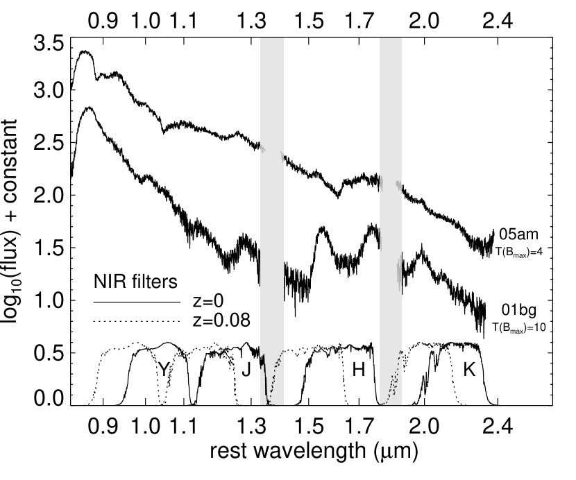
Figure 1: NIR spectra of the normal Type Ia SNe 2005am and 2001bg obtained $+$4 and $+$10 days relative to $T(B_{\rm max}$), respectively. Also plotted as black lines are the rest-frame CSP natural system NIR transmission functions. In addition, these passbands are also plotted as dotted lines at the locations which cover the SED they sample when observing a SN Ia at $z=0.08$. The vertical bands correspond to regions containing prevalent telluric absorption.

In what follows we adopt for $S_{i}(\lambda)$ the $YJHK_{s}$ passbands of the Carnegie Supernova Project (CSP; Hamuy et al. 2006). Currently the CSP relies on modeled NIR instrumental passbands which have been constructed by multiplying together the factory-measured filter transmissivities with the transmission functions of two generic mirror reflections, various optical elements, a HAWAII–1 1024 $\times$ 1024 pixel HgCdTe detector response curve and a telluric absorption spectrum (Hamuy et al., 2006). The modeled passbands are electronically available on the CSP webpage, and are plotted in Figure 1, along with NIR spectra of the normal Type Ia SNe 2005am and 2001bg obtained $+$4 and $+$10 days past $B$-band maximum (hereafter $T(B_{\rm max}$)), respectively. This comparison highlights the prevalent emission features that coincide with the position of the rest-frame $H$ band, which emerge and increase to maximum strength within the first two weeks past maximum. To illustrate the effect of cosmological redshift each passband is plotted at rest and at the positions corresponding to the wavelength regions of the SED they sample at $z=$ 0.08.

3 METHODS

3.1 NIR Spectral Data

Our analysis is based on 75 published NIR spectra of 33 SNe Ia that cover the $YJHK_{s}$ bands. The temporal range spanned is from $-$14.6 to $+$53.8 days relative to $T(B_{\rm max}$). The majority of the data are drawn from the Marion et al. (2009) catalog, which were obtained between 2000 and 2005 with the NASA Infrared Telescope Facility (IRTF) equipped with SpeX, a medium-resolution, NIR spectrograph and imager. Additional spectra include the published sequences of SN 1999ee (Hamuy et al., 2002), SN 2003du (Stanishev et al., 2007), SN 2005cf (Gall et al., 2012) and SN 2011fe (Hsiao et al., 2013). Table 1 lists each spectrum sorted by phase along with its date of observation, the telescope used to make the observations, the redshift of each host galaxy as given by NED, and an estimate of $\Delta$$m_{15}(B)$ for each object. When possible, the reported phase of a spectrum was estimated with respect to $T(B_{\rm max}$)  measured from its $B$-band light curve. However, there are a fews cases where no light curve information is available, we therefore estimated $T(B_{\rm max}$) by cross-correlating an optical spectrum to a library of SN Ia spectra using the Supernova Identification (SNID) code (Blondin & Tonry 2007). In these instances, the estimated temporal phase with respect to $T(B_{\rm max}$)  has a realistic uncertainty of $\pm$3 days (Blondin & Tonry, 2007).

3.2 Assigning Proper Errors

Before $K$ corrections can be calculated, the errors associated with the spectra must be quantified. These arise from two principal sources: signal-to-noise of the spectrum, and improperly removed telluric features, which are especially important to account for at NIR wavelengths. In the first case, we used the associated error spectrum when this was available. Otherwise, an estimate of the signal-to-noise as a function of wavelength was made for each spectrum, typically amounting to 10% of the signal. Due to the fact that this is uncorrelated noise, its effect on the uncertainty of the $K$ corrections is relatively small.

Errors in the telluric corrections can arise from several factors, but typically are due to rapid changes in the water vapor conditions. Also, for some features, the absorption reaches 100% of the continuum. These errors become important at higher redshifts when the features are shifted into the filter bandpasses. Unlike the errors due to signal-to-noise, these telluric correction errors can be highly correlated if improperly subtracted. Fortunately, most spectra showed no sign of any systematic over- or under-subtraction, in which case we treated the error as white noise. Only in the cases where removal of the features left a clear imprint on the corrected spectrum did we simulate an additional error using a telluric template spectrum.

These two errors were then propagated using Monte Carlo simulations. In brief, 100 artificial spectra were created by introducing noise at a level consistent with the dispersion of the above-described errors, resulting in a sample of 100 $K$ corrections. The standard deviation was then computed and adopted as the final error in the $K$ correction for the particular redshift being calculated.

3.3 Extending the Wavelength Coverage of the Input Spectra

The goal of this paper is to quantify the errors in the $K$ corrections due to variations in spectral features (cf. Hsiao et al., 2007). Our approach is to color-match the sample spectra to observed colors derived from the Hsiao revised template at a range of redshifts. The procedures used for the color-matching are those described by Hsiao et al. (2007) and Burns et al. (2011).

Ideally, when calculating $K$ corrections for a particular supernova, multiple observed colors will be available spanning an extended wavelength range so as to properly anchor the color-matching function. However, in the present paper, we are dealing with spectral observations with limited wavelength coverage. Hence, it is necessary to extend the sample spectra to bluer and redder wavelengths. First, for each observed spectrum, the Hsiao revised template is color-matched to synthetic colors calculated from the observed spectrum. The color-matched template spectrum was then scaled to match the integrated flux under the bluest (or reddest, in the case of the $K_{s}$ band) filter covered by the observed spectrum. The template and observed spectra are then combined utilizing an overlapping 300 Å  region with appropriate weighting. Note that the extended sections are not used in the $K$-correction calculations, but serve only for color matching.

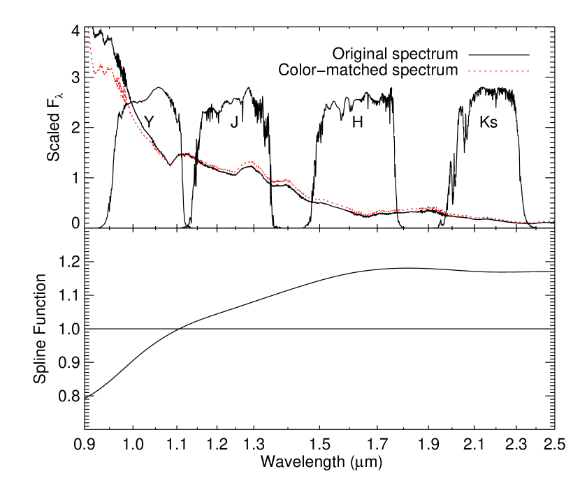
Figure 2: (top panel) Comparison of the maximum light spectrum of SN 2011fe (solid black line) to its altered version (dotted red line) that is matched to the observed colors derived from the Hsiao revised spectral template at $z=0.03$. Overplotted in the top panel are the CSP $YJHK_{s}$ passbands at rest wavelength. (bottom panel) The spline function used to perform the color matching of the input spectrum to match the colors calculated from the Hsiao revised spectral template.

An example of an original and color-matched spectrum of a normal SN Ia that has been extrapolated in the blue is shown in Figure 2.

3.4 Gaussian Process and MCMC modeling

We have adopted a Bayesian formalism to compute an interpolated function of the $K$ term as a function of light-curve phase, redshift, and filter, along with a robust estimate of its uncertainty, which is more accurate than what is obtained by just simply binning residuals, particularly in the presence of outliers. In this manner the computed error snake is a combination of (i) observational error, (ii) the differing number of points constraining the interpolator at any particular phase and redshift, and (iii) intrinsic differences between individual SN Ia. These last two errors are particularly difficult to disentangle, prompting us to opt for a combined Gaussian Process and Markov-Chain Monte-Carlo (MCMC) method to obtain an empirically-based model and an associated error estimate.

Gaussian Processes (Rasmussen & Williams, 2006) are a generalization of probability distributions for functions. Instead of a mean value, one solves for a mean function, $F(t)$, and in addition, a covariance function, [$C(t_{1},t_{2})$]. The covariance function is a generalization of the standard deviation of a Gaussian distribution and encapsulates the uncertainty in the mean function. While the mean function is non-parametric, we elected to use the Matérn covariance function (Banerjee, Carlin & Gelfand, 2003), which has four parameters: scale ($s$), amplitude ($\theta$), the degree of differentiability ($d$), and an intrinsic variance ($\sigma_{var}$). The value of $s$ sets the scale over which departures from the mean function are coherent, while $\theta$ determines the size of these departures, $d$ controls the degree of differentiability (or smoothness) of the function, and $\sigma_{var}$ characterizes any additional uncorrelated dispersion of the interpolated function that exceeds the uncertainty of the $K$ corrections. To implement this approach, the python package PyMC (Patil, Huard, & Fonnesbeck, 2010) was used to compute the best values for $s$, $\theta$, $d$, and $\sigma_{var}$, as well as $F(t)$ via the MCMC method.

The advantage of MCMC modeling is that it allows one to marginalize over the adopted assumptions and missing information, and at the same time provides a robust error snake. At each MCMC step, $s$, $\theta$ and $d$ are proposed and a Gaussian Process is computed which gives an interpolation between the observed $K$ corrections. The residuals between the observed points and the interpolated function are then determined. If the residuals are consistent with the errors of the individual $K$ corrections, then the MCMC process has found a higher likelihood state. If the residuals are larger than the errors, a lower likelihood state is obtained. The Metropolis-Hastings algorithm is used to propose each new MCMC step, randomly walking through parameter space, though converging to higher probability states. There are two states where the likelihood is locally maximized: (i) $s$ and $d$ are small, $\theta$ is large, and the interpolator fits the noise; and (ii) $s$ and $d$ are larger, $\theta$ smaller, and the interpolator smoothly fits the data, though with larger scatter than the errors in the data should allow. Introducing the extra noise term $\sigma_{var}$ gives the second case a higher probability and also gives us an estimate of the intrinsic scatter in the $K$ corrections.

Once the Markov chain has converged, all the states are tallied, and for each state, $i$, the interpolating function, $F_{i}(t)$, is computed. The median of all $F_{i}(t)$ represents the final $F(t)$, while the standard deviation of the interpolations gives the “error in the mean” function, which we refer to in the following as $\sigma_{stat}$. Due to the varying density of data points used to constrain the interpolation, the value of $\sigma_{stat}$ varies with both redshift and temporal phase. The computed value of $\sigma_{var}$ is held constant for each redshift bin since, given the size of the current library of NIR spectra, there simply is not enough data to obtain an estimate as a function of temporal phase. We are unable to directly attribute $\sigma_{var}$ to any one variable, but this parameter most likely reflects intrinsic SN-to-SN differences such as spectral line diversity. It is our view that a combination of both noise terms ($\sigma_{stat}$ and $\sigma_{var}$) represents the most appropriate error snakes to adopt if one intends to include the $K$-term uncertainty in the overall error budget of cosmological parameters derived from NIR observations of SNe Ia.

4 RESULTS

Armed with the $YJHK_{s}$ passbands shown in Figure 1 and our adopted library of NIR SN Ia spectra (see Table 1), $K$ corrections were computed using Equation (2) for redshifts of $z=0.03,0.05,0.08$. The arrays of $K$ corrections for each of these redshift intervals were then fed into our MCMC algorithm, from which smooth mean functions were computed. The definitive $K$-correction interpolations and their associated values of $\sigma_{stat}$ are provided in Table 2. Listed in Table 3 are the computed values of $\sigma_{var}$, which dominate the total errors for all four passbands near maximum light.

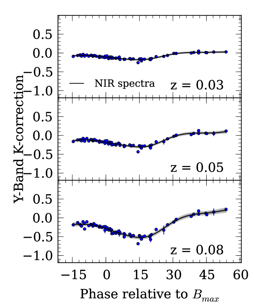
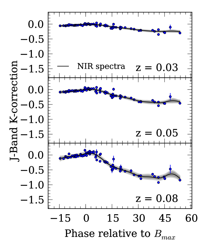
Figure 3: $K$ corrections in the $YJHK_{s}$ bandpasses (blue points) computed from 75 NIR SN Ia spectra at $z=0.03$, 0.05, 0.08. Solid black line corresponds to MCMC interpolated functions, while dark and light shaded regions correspond to $\sigma_{stat}$, and the summation in quadrature of $\sigma_{stat}$ and $\sigma_{var}$, respectively.

Illustrations of the computed $K$ corrections and their mean interpolated functions as a function of temporal phase are presented in Figure 3 for the three adopted redshifts. In each panel the points correspond to the individual $K$ corrections derived from Equation (2). The solid black lines are the MCMC mean functions, and the shaded regions are confidence levels of these functions. The darker of the two shaded regions corresponds to $\sigma_{stat}$, while the less dark regions are obtained through the summation in quadrature of $\sigma_{stat}$ and $\sigma_{var}$. As expected, the overall evolution of the $K$ terms in $Y$, $J$, and $H$ as a function of phase, mimic to first order the evolution of the $(Y-J)$, $(J-H)$, and $(H-K)$ color curves.

We would emphasize that the $K$ terms given in Table 2 are listed for reference only, and should not be used blindly to correct NIR photometry for any given SN. Rather, we recommend a two-step process. The chosen spectral template template should first be color-matched to the SN photometry and then used to calculate $K$ corrections for the filter bandpasses employed. The uncertainties given in Tables 2 and 3 should then be interpolated to the redshift of the SN and propagated as part of the $K$-correction process. As mentioned in §3.4, we recommend summing in quadrature the values of $\sigma_{stat}$ and $\sigma_{var}$ to estimate the total error in the $K$ correction.

In the remainder of this section, we discuss results for each of the four CSP filter bandpasses.

4.1 $Y$ and $J$ Filters

Figure 3 shows that, of the four CSP bandpasses, $Y$ yields the lowest $K$-correction uncertainties. This is due in large part to the fact that this wavelength region does not develop any strong spectral features until $\sim$30 days after $T(B_{\rm max}$) (see Figure 9 of Marion et al., 2009). This is reflected in the relatively small increase $\sigma_{var}$ from $\pm 0.02$ to $\pm 0.04$ mag between $z=0.03$ and 0.08 (see Table 3 and Figure 4). Moreover, the $Y$ band is not affected by strong telluric absorption, and is generally characterized by higher signal-to-noise than any of the other NIR bandpasses. The small $K$-correction uncertainties combined with an essentially negligible dependence of absolute magnitude on decline rate (Kattner et al., 2012) and low sensitivity to dust extinction make the $Y$ band an interesting option for future cosmological studies. Note, however, that to obtain the highest precision in the $Y$ band, it is important that the photometric coverage of the SN extend to at least the $i$ (or $I$) filter since this is essential for proper color-matching of the spectral template.

The $K$-correction models indicate that the $J$ passband is also characterized by relatively small uncertainties, although not quite at the low levels observed for the $Y$ band. The statistical errors of the $J$-band $K$ terms are slightly higher than those for $Y$ and, as indicated in Table 3 and illustrated in Figure 4, the uncertainties due to intrinsic spectral variations are also $\sim$50% greater. Nevertheless, the $J$ filter clearly offers considerable promise for cosmological studies.

4.2 $H$ Filter

Kasen (2006) has argued from theoretical grounds that the spread in the absolute magnitudes of SNe Ia should decrease steadily from the optical to the NIR, reaching a minimum dispersion of $\sim\pm 0.1$ mag at $H$, and Wood-Vasey et al. (2008) concluded the same based on observations of 21 SNe Ia in in $JHK$. Nevertheless, Figure 3 shows that the dispersion in the $H$-band $K$ corrections increases much more sharply with redshift than for the $Y$ and $J$ filters, with the error snakes indicating that the increases occur in both $\sigma_{stat}$ and $\sigma_{var}$. The increase in $\sigma_{stat}$ is predictable since the library spectra all correspond to low-redshift ($z\lesssim 0.03$) SNe. As illustrated in Figure 1, the wavelength region of the library spectra affected by the telluric absorption band at 1.34-1.41 $\mu$m is shifted more and more into the blue edge of the $H$ passband at increasing redshift, introducing increasing levels of noise into the $K$-correction calculation due to errors in the telluric corrections. These statistical errors can be beaten down as NIR spectra are obtained of SNe Ia at a larger range of redshifts.

As shown in Figure 4, the increase in $\sigma_{var}$ with redshift for the $H$ band is greater than that suffered by any of the other CSP NIR filters, reaching a value of nearly $\pm 0.1$ mag at $z=0.08$. This behavior is most likely the result of intrinsic diversity in the strong iron-peak emission features that strengthen dramatically in the $H$ band beginning only a few days after $T(B_{\rm max}$) (Wheeler et al., 1998). Hsiao et al. (2013) recently studied the strength of the “break” at $\sim$1.5 $\mu$m, and found evidence that it correlates with $\Delta m_{15}(B)$. If confirmed, it should be possible to eventually decrease $\sigma_{var}$ by creating NIR spectral templates in the $H$ band that are a function of $\Delta m_{15}(B)$. This, however, will require a much larger library of NIR spectral observations.

4.3 $K_{s}$ Filter

In principle, the $K_{s}$ bandpass also offers significant advantages for measuring cosmological distances. Dust extinction is lowest at this wavelength, and the increase of $\sigma_{var}$ with redshift is only $\pm 0.01$ mag greater than derived for the $J$ band (see Table 3 and Figure 4). However, the signal-to-noise typically achieved in the $K_{s}$ band is less than in the other NIR filters (see Figure 9 of Marion et al., 2009). This is due to both the faintness of the SNe and the much stronger sky emission encountered at these longer wavelengths. Secondly, similar to the $H$ band, $K$-correction calculations for the $K_{s}$ filter suffer from redshift-dependent noise introduced by the strong telluric absorption band at 1.8-1.9 $\mu$m (see Figure 1) although, again, it should be possible to minimize the impact of this effect as NIR spectra of SNe Ia are obtained over a larger range of redshifts. A final disadvantage of the $K_{s}$ bandpass is the difficulty of properly color-matching it to a spectral template since observations are not generally available in a longer-wavelength filter to help anchor the correction.

5 CONCLUSIONS

Using a library of publicly available SNe Ia NIR spectra, we have computed a set of $K$ corrections in the CSP $YJHK_{s}$ filters at redshifts of $z=0.03$, 0.05, and 0.08. The individual spectra were first color-matched to the Hsiao revised spectral template before calculating the $K$ corrections. A combined Gaussian Process and MCMC method was then employed to derive an empirically-based model of the $K$ terms as a function of temporal phase and redshift. This procedure returns uncertainties in the $K$-correction model due to both statistical noise and intrinsic diversity in the features of the input spectra.

Krisciunas et al. (2004) published a table of NIR $K$ corrections computed using spectra of SN 1999ee, and a set of filters functions similar to those adopted in this study. A comparison between the results of Krisciunas et al. to those obtained with our expanded set of spectra and more advanced color-matching technique provides good agreement in the $J$ and $H$ bands at $z=0.03$, while for the $K_{s}$ band we find differences of up to $\pm$0.08 mag. The discrepancy in the $K_{s}$ is not surprising owing the the dearth of spectra included in the work of Krisciunas et al., as well as the difficulties highlighted in this study concerning the difficulties inherent to computing robust $K_{s}$-band $K$ corrections.

Our emphasis in this paper has not been to provide “lookup” tables of NIR $K$ corrections, but rather to derive accurate estimates of the uncertainties inherent in the use of spectral templates (like the Hsiao revised template) constructed from the NIR sample of SNe Ia spectra available today. We find that the $Y$ and $J$ bands currently afford the greatest precision in $K$-correction calculations due to the general weakness of the spectral features and the minimal effect of telluric corrections. The $Y$ band is particularly noteworthy, with the uncertainty due to spectral feature variations increasing from only $\pm 0.02$ to $\pm$0.04 mag from $z=0.03$–0.05. The $H$ band is currently more problematic due to noise introduced by telluric corrections and the appearance just after maximum light of strong Fe-peak emission features. Diversity in the strength of this emission most likely explains the strong increase we find in the intrinsic component of the $K$-correction error from $\pm 0.02$ to $\pm$0.10 mag over the redshift range $z=0.03$–0.05. This result is a departure from pervious theoretical (Kasen, 2006) and observational (Wood-Vasey et al., 2008) findings, which have identified the $H$ band as having potentially the least dispersion among the NIR passbands. Finally, the uncertainties in the $K$ terms for the $K_{s}$ filter due to intrinsic spectral diversity are similar to those found for the $J$ band, but the currently-available library of spectra covering this wavelength region suffer from both low signal-to-noise and telluric absorption.

Further progress in reducing the uncertainties in the $K$ corrections for NIR filter bandpasses demands many more spectral observations over a wider range of redshifts. Figure 5 shows a histogram of the decline rates of the SNe Ia in our sample with temporal phases within $\pm 3$ days of $T(B_{\rm max}$). For reference, the same figure includes a plot of the decline rates of the spectra employed by Hsiao et al. (2007) to create their optical spectral template. The discrepancy between these two histograms dramatically illustrates the limitations of the currently-available library of NIR spectra. To address this problem, we have embarked on a four-year, six-months-a-year SN Ia followup program that builds upon the legacy of the CSP. This project, designated CSP-II, is designed to obtain optical and NIR light-curves of $\sim$100 SNe Ia in the smooth Hubble flow ($0.03<z<0.08$). Complementary to these observations, frequent NIR spectroscopy is being carried out of nearby SNe Ia, mainly with the Folded-port InfraRed Echellette (FIRE) spectrograph mounted on the 6.5-m Magellan Baade telescope. Particular emphasis is being placed on obtaining spectral sequences for a sub-sample of the SNe that span a range in decline rate and phase, which are essential to determining correlated errors in the $K$ corrections. We are confident that such observations will not only allow us to more precisely characterize NIR $K$-correction uncertainties, but also to decrease these errors to the low levels now obtained at optical wavelengths.

In order to ascertain the contribution of NIR $K$-correction errors to the final error budget of cosmological parameters one must determine whether they are systematic in temporal phase, and therefore propagate to the peak magnitude of a SN Ia. On the other hand, if the $K$-correction errors are random in phase then the final uncertainty in the peak magnitude will be reduced by template fitting. To determine which of these is the case is, however, beyond the scope of this paper due to the lack of a statistical sample of SNe Ia with good spectral time series. However, in the near future we will be able to tackle this issue with the high-fidelity spectral series currently being obtained.

Figure 4: Plot of the uncertainties due most likely to spectral diversity, $\sigma_{var}$, versus redshift.

Figure 5: Histogram of the decline rates of the published NIR spectra of SNe Ia in our sample obtained within $\pm 3$ days of $T(B_{\rm max}$). A comparable histogram for the optical spectra in the Hsiao et al. (2007) template over the same range of epochs is shown for comparison.

Table 1: Seventy-five NIR SN Ia spectra sorted by phase

SN	Epoch	Obs. Date	Telescope	Redshift	$\Delta m_{15}$
	$T(B_{max})$	(UT)		Host ($z$)	($B$)
2011fe	$-$14.6(0.5)	Aug. 26.3	IRTF	0.0008	1.078
2011fe	$-$12.6(0.5)	Aug. 28.3	Gem-N	0.0008	1.078
2003du	$-$11.5(0.5)	Apr. 25.0	UKIRT	0.0064	1.026
2002fk	$-$11.3(0.5)	Sep. 19.4	IRTF	0.0071	1.083
2003du	$-$10.9(0.5)	Apr. 25.9	TNG	0.0064	1.026
2005cf	$-$10.2(0.5)	Jun. 01.1	VLT	0.0065	1.129
2011fe	$-$09.7(0.5)	Aug. 31.2	Gem-N	0.0008	1.078
2005cf	$-$09.5(0.5)	Jun. 03.1	TNG	0.0065	1.129
1999ee	$-$08.5(0.5)	Oct. 09.0	VLT	0.0114	0.947
2004bw	$-$07.7(0.5)	May 30.4	IRTF	0.0214	1.313
2011fe	$-$06.7(0.5)	Sep. 03.2	Gem-N	0.0008	1.078
2003W	$-$06.5(0.5)	Feb. 02.4	IRTF	0.0201	1.165
2002cr	$-$05.9(0.5)	May 08.4	IRTF	0.0096	1.265
2000dn	$-$05.8(0.5)	Oct. 01.5	IRTF	0.0320	1.123
2003du	$-$05.5(0.5)	May 01.0	UKIRT	0.0064	1.026
2003W	$-$05.5(0.5)	Feb. 03.4	IRTF	0.0201	1.165
2005cf	$-$05.4(0.5)	Jun. 06.1	VLT	0.0065	1.129
2004bv	$-$05.0(0.5)	May 30.5	IRTF	0.0105	0.893
2002cr	$-$04.2(0.5)	May 10.1	IRTF	0.0096	1.265
2005am	$-$02.9(0.5)	Mar. 05.3	IRTF	0.0079	0.782
2011fe	$-$02.8(0.6)	Sep. 07.1	Gem-N	0.0008	1.078
2002hw	$-$02.6(0.5)	Nov. 14.3	IRTF	0.0175	1.515
2002el	$-$01.8(0.5)	Aug. 20.5	IRTF	0.0233	1.393
2001br	$-$00.9(0.6)	May 22.6	IRTF	0.0206	0.933
2004bl	$-$00.4(3.7)	May 08.3	IRTF	0.0173	$\cdots$
2005cf	$-$00.3(0.5)	Jun. 11.1	VLT	0.0065	1.129
2011fe	$+$00.3(0.5)	Sep. 10.2	Gem-N	0.0008	1.078
1999ee	$+$00.5(0.5)	Oct. 18.0	NTT	0.0114	0.947
2005am	$+$01.2(0.5)	Mar. 09.4	IRTF	0.0079	0.782
1999ee	$+$01.5(0.5)	Oct. 19.0	VLT	0.0114	0.947
2005cf	$+$01.8(0.5)	Jun. 13.1	VLT	0.0065	1.129
2000dm	$+$02.3(0.6)	Oct. 01.2	IRTF	0.0153	1.563
2001dl	$+$02.5(0.5)	Aug. 12.5	IRTF	0.0207	0.983
2003du	$+$02.7(0.5)	May 09.3	IRTF	0.0168	1.026
2011fe	$+$03.3(0.5)	Sep. 13.2	Gem-N	0.0008	1.078
2003du	$+$04.5(0.5)	May 11.0	UKIRT	0.0064	1.026
1999ee	$+$04.5(0.5)	Oct. 22.1	NTT	0.0114	0.947
2001bf	$+$05.7(0.5)	May 21.5	IRTF	0.0155	0.933
2004da	$+$06.0(3.0)	Jul. 08.5	IRTF	0.0163	0.874
2000do	$+$06.2(3.0)	Oct. 02.2	IRTF	0.0109	$\cdots$
2000dk	$+$06.3(0.5)	Oct. 01.5	IRTF	0.0174	1.631
2005am	$+$08.2(0.5)	Mar. 16.4	IRTF	0.0079	0.782
2011fe	$+$08.2(0.5)	Sep. 18.3	Gem-N	0.0008	1.078
1999ee	$+$08.5(0.5)	Oct. 26.0	NTT	0.0114	0.947
2005cf	$+$10.7(0.5)	Jun. 22.1	VLT	0.0065	1.129
2002ha	$+$11.3(0.5)	Nov. 14.2	IRTF	0.0141	1.345
2001bg	$+$11.3(0.5)	May 22.2	IRTF	0.0071	1.103
2011fe	$+$12.3(0.5)	Sep. 22.2	Gem-N	0.0008	1.078
2005cf	$+$14.4(0.5)	Jun. 27.1	TNG	0.0065	1.129
2004ab	$+$15.0(3.0)	Mar. 07.5	IRTF	0.0058	$\cdots$
2005am	$+$15.1(0.5)	Mar. 23.3	IRTF	0.0079	0.782
2003du	$+$15.4(0.5)	May 22.0	TNG	0.0064	1.026
1999ee	$+$15.5(0.5)	Nov. 02.0	VLT	0.0114	0.947
2002ef	$+$15.6(0.6)	Aug. 20.6	IRTF	0.0240	1.043
2004da	$+$15.9(3.0)	Jul. 18.4	IRTF	0.0163	0.874
2003du	$+$16.2(0.5)	May 23.1	TNG	0.0064	1.026
2011fe	$+$17.3(0.5)	Sep. 27.2	Gem-N	0.0008	1.078
2004bk	$+$19.7(0.7)	May 08.5	IRTF	0.0230	1.183
2001en	$+$19.8(0.5)	Oct. 30.3	IRTF	0.0159	1.273
2004da	$+$20.0(3.0)	Jul. 22.5	IRTF	0.0163	0.874
2003du	$+$20.4(0.5)	May 27.0	UKIRT	0.0064	1.026
1999ee	$+$22.5(0.5)	Nov. 09.0	NTT	0.0114	0.947
2004da	$+$25.9(3.0)	Jul. 28.4	IRTF	0.0163	0.874
1999ee	$+$27.6(0.5)	Nov. 14.1	NTT	0.0114	0.947
2003du	$+$30.4(0.5)	Jun. 06.0	UKIRT	0.0064	1.026
2005cf	$+$31.4(0.5)	Jul. 14.1	TNG	0.0065	1.129
1999ee	$+$31.5(0.5)	Nov. 18.0	VLT	0.0114	0.947
2004E	$+$38.2(2.5)	Feb. 21.5	IRTF	0.0298	1.273
2003cg	$+$39.3(0.5)	May 09.2	IRTF	0.0041	1.251
1999ee	$+$41.5(0.5)	Nov. 28.0	VLT	0.0114	0.947
2005cf	$+$41.5(0.5)	Jul. 24.0	TNG	0.0065	1.129
2002fk	$+$44.8(0.5)	Nov. 14.4	IRTF	0.0071	1.083
2004ca	$+$45.1(3.0)	Jul. 28.6	IRTF	0.0173	$\cdots$
2001gc	$+$48.3(5.5)	Jan. 14.5	IRTF	0.0193	1.285
2004bv	$+$53.8(0.5)	Jul. 28.3	IRTF	0.0105	0.893

Table 2: $YJHK_{s}$$-$band $K$ corrections at $z=0.03,0.05,0.08$

Phase	$Y$	$\sigma_{stat}$	$J$	$\sigma_{stat}$	$H$	$\sigma_{stat}$	$K_{s}$	$\sigma_{stat}$
$z=0.03$
-14.6	-0.075	$\pm$0.011	-0.061	$\pm$0.016	-0.050	$\pm$0.016	-0.024	$\pm$0.017
-13.9	-0.072	$\pm$0.009	-0.059	$\pm$0.014	-0.049	$\pm$0.013	-0.026	$\pm$0.015
-13.2	-0.070	$\pm$0.008	-0.057	$\pm$0.012	-0.048	$\pm$0.011	-0.028	$\pm$0.013
-12.5	-0.068	$\pm$0.007	-0.055	$\pm$0.011	-0.046	$\pm$0.010	-0.030	$\pm$0.011
-11.8	-0.066	$\pm$0.006	-0.053	$\pm$0.010	-0.044	$\pm$0.008	-0.033	$\pm$0.010
-11.1	-0.065	$\pm$0.005	-0.051	$\pm$0.009	-0.042	$\pm$0.008	-0.036	$\pm$0.008
-10.5	-0.065	$\pm$0.005	-0.048	$\pm$0.008	-0.040	$\pm$0.007	-0.039	$\pm$0.008
-9.8	-0.065	$\pm$0.005	-0.046	$\pm$0.008	-0.038	$\pm$0.007	-0.043	$\pm$0.008
-9.1	-0.065	$\pm$0.005	-0.044	$\pm$0.008	-0.037	$\pm$0.007	-0.047	$\pm$0.007
-8.4	-0.067	$\pm$0.004	-0.041	$\pm$0.007	-0.035	$\pm$0.007	-0.051	$\pm$0.007
-7.7	-0.068	$\pm$0.004	-0.039	$\pm$0.007	-0.033	$\pm$0.006	-0.056	$\pm$0.007
-7.0	-0.071	$\pm$0.004	-0.037	$\pm$0.007	-0.032	$\pm$0.006	-0.061	$\pm$0.007
-6.3	-0.074	$\pm$0.004	-0.034	$\pm$0.007	-0.031	$\pm$0.006	-0.066	$\pm$0.007
-5.6	-0.077	$\pm$0.004	-0.032	$\pm$0.007	-0.030	$\pm$0.006	-0.072	$\pm$0.007
-4.9	-0.080	$\pm$0.004	-0.030	$\pm$0.007	-0.030	$\pm$0.006	-0.078	$\pm$0.007
-4.2	-0.084	$\pm$0.004	-0.027	$\pm$0.007	-0.029	$\pm$0.006	-0.084	$\pm$0.007
-3.5	-0.088	$\pm$0.004	-0.024	$\pm$0.007	-0.028	$\pm$0.006	-0.090	$\pm$0.007
-2.9	-0.092	$\pm$0.004	-0.022	$\pm$0.007	-0.028	$\pm$0.006	-0.096	$\pm$0.007
-2.2	-0.096	$\pm$0.004	-0.019	$\pm$0.007	-0.026	$\pm$0.006	-0.103	$\pm$0.007
-1.5	-0.101	$\pm$0.004	-0.016	$\pm$0.006	-0.024	$\pm$0.006	-0.109	$\pm$0.007
-0.8	-0.105	$\pm$0.004	-0.014	$\pm$0.006	-0.022	$\pm$0.006	-0.115	$\pm$0.007
-0.1	-0.109	$\pm$0.004	-0.012	$\pm$0.007	-0.018	$\pm$0.006	-0.121	$\pm$0.007
0.6	-0.113	$\pm$0.004	-0.011	$\pm$0.007	-0.013	$\pm$0.006	-0.127	$\pm$0.007
1.3	-0.117	$\pm$0.004	-0.010	$\pm$0.007	-0.007	$\pm$0.006	-0.132	$\pm$0.007
2.0	-0.122	$\pm$0.004	-0.009	$\pm$0.007	0.000	$\pm$0.006	-0.137	$\pm$0.007
2.7	-0.126	$\pm$0.004	-0.010	$\pm$0.007	0.009	$\pm$0.006	-0.142	$\pm$0.007
3.4	-0.130	$\pm$0.004	-0.010	$\pm$0.007	0.019	$\pm$0.006	-0.146	$\pm$0.007
4.1	-0.134	$\pm$0.004	-0.012	$\pm$0.008	0.031	$\pm$0.006	-0.149	$\pm$0.007
4.7	-0.139	$\pm$0.004	-0.014	$\pm$0.008	0.043	$\pm$0.006	-0.151	$\pm$0.007
5.4	-0.143	$\pm$0.004	-0.016	$\pm$0.008	0.057	$\pm$0.006	-0.153	$\pm$0.008
6.1	-0.147	$\pm$0.005	-0.019	$\pm$0.008	0.072	$\pm$0.006	-0.154	$\pm$0.008
6.8	-0.151	$\pm$0.005	-0.023	$\pm$0.008	0.087	$\pm$0.007	-0.155	$\pm$0.008
7.5	-0.154	$\pm$0.005	-0.027	$\pm$0.008	0.101	$\pm$0.007	-0.154	$\pm$0.008
8.2	-0.158	$\pm$0.005	-0.031	$\pm$0.008	0.116	$\pm$0.008	-0.153	$\pm$0.008
8.9	-0.162	$\pm$0.005	-0.036	$\pm$0.008	0.129	$\pm$0.008	-0.152	$\pm$0.008
9.6	-0.165	$\pm$0.005	-0.042	$\pm$0.007	0.141	$\pm$0.009	-0.149	$\pm$0.008
10.3	-0.168	$\pm$0.005	-0.048	$\pm$0.007	0.151	$\pm$0.009	-0.146	$\pm$0.009
11.0	-0.171	$\pm$0.005	-0.054	$\pm$0.007	0.159	$\pm$0.009	-0.142	$\pm$0.008
11.7	-0.173	$\pm$0.005	-0.061	$\pm$0.008	0.165	$\pm$0.009	-0.137	$\pm$0.008
12.3	-0.175	$\pm$0.005	-0.067	$\pm$0.008	0.168	$\pm$0.009	-0.132	$\pm$0.008
13.0	-0.177	$\pm$0.005	-0.074	$\pm$0.009	0.170	$\pm$0.009	-0.126	$\pm$0.008
13.7	-0.178	$\pm$0.005	-0.080	$\pm$0.009	0.169	$\pm$0.008	-0.120	$\pm$0.008
14.4	-0.179	$\pm$0.005	-0.086	$\pm$0.009	0.168	$\pm$0.008	-0.114	$\pm$0.008
15.1	-0.179	$\pm$0.005	-0.092	$\pm$0.009	0.165	$\pm$0.008	-0.107	$\pm$0.008
15.8	-0.178	$\pm$0.005	-0.097	$\pm$0.009	0.161	$\pm$0.008	-0.100	$\pm$0.008
16.5	-0.176	$\pm$0.005	-0.103	$\pm$0.008	0.157	$\pm$0.008	-0.092	$\pm$0.008
17.2	-0.173	$\pm$0.005	-0.108	$\pm$0.008	0.153	$\pm$0.008	-0.085	$\pm$0.008
17.9	-0.170	$\pm$0.005	-0.113	$\pm$0.008	0.148	$\pm$0.008	-0.078	$\pm$0.008
18.6	-0.165	$\pm$0.006	-0.118	$\pm$0.008	0.144	$\pm$0.008	-0.070	$\pm$0.009
19.2	-0.160	$\pm$0.006	-0.122	$\pm$0.008	0.139	$\pm$0.008	-0.063	$\pm$0.009
19.9	-0.154	$\pm$0.006	-0.127	$\pm$0.009	0.135	$\pm$0.009	-0.056	$\pm$0.010
20.6	-0.147	$\pm$0.006	-0.131	$\pm$0.009	0.131	$\pm$0.009	-0.049	$\pm$0.010
21.3	-0.140	$\pm$0.006	-0.136	$\pm$0.010	0.128	$\pm$0.009	-0.042	$\pm$0.010
22.0	-0.132	$\pm$0.007	-0.140	$\pm$0.011	0.125	$\pm$0.010	-0.036	$\pm$0.010
22.7	-0.123	$\pm$0.007	-0.145	$\pm$0.012	0.122	$\pm$0.010	-0.030	$\pm$0.011
23.4	-0.114	$\pm$0.007	-0.149	$\pm$0.012	0.119	$\pm$0.011	-0.024	$\pm$0.011
24.1	-0.105	$\pm$0.007	-0.154	$\pm$0.013	0.116	$\pm$0.011	-0.018	$\pm$0.012
24.8	-0.095	$\pm$0.007	-0.159	$\pm$0.013	0.113	$\pm$0.011	-0.013	$\pm$0.012
25.5	-0.086	$\pm$0.007	-0.164	$\pm$0.013	0.110	$\pm$0.011	-0.008	$\pm$0.012
26.2	-0.077	$\pm$0.007	-0.169	$\pm$0.013	0.107	$\pm$0.011	-0.003	$\pm$0.012
26.8	-0.068	$\pm$0.007	-0.174	$\pm$0.012	0.103	$\pm$0.011	0.001	$\pm$0.012
27.5	-0.059	$\pm$0.007	-0.179	$\pm$0.012	0.099	$\pm$0.011	0.005	$\pm$0.013
28.2	-0.050	$\pm$0.007	-0.185	$\pm$0.012	0.095	$\pm$0.011	0.008	$\pm$0.013
28.9	-0.042	$\pm$0.007	-0.190	$\pm$0.012	0.090	$\pm$0.011	0.012	$\pm$0.013
29.6	-0.034	$\pm$0.007	-0.195	$\pm$0.012	0.085	$\pm$0.011	0.014	$\pm$0.013
30.3	-0.027	$\pm$0.008	-0.200	$\pm$0.012	0.079	$\pm$0.011	0.017	$\pm$0.013
31.0	-0.020	$\pm$0.008	-0.204	$\pm$0.012	0.074	$\pm$0.011	0.019	$\pm$0.013
31.7	-0.014	$\pm$0.008	-0.209	$\pm$0.012	0.069	$\pm$0.011	0.020	$\pm$0.013
32.4	-0.009	$\pm$0.008	-0.213	$\pm$0.013	0.064	$\pm$0.012	0.021	$\pm$0.014
33.1	-0.004	$\pm$0.009	-0.216	$\pm$0.014	0.059	$\pm$0.012	0.022	$\pm$0.014
33.8	-0.000	$\pm$0.009	-0.220	$\pm$0.015	0.055	$\pm$0.013	0.023	$\pm$0.014
34.4	0.003	$\pm$0.009	-0.223	$\pm$0.016	0.052	$\pm$0.014	0.023	$\pm$0.014
35.1	0.006	$\pm$0.009	-0.227	$\pm$0.016	0.049	$\pm$0.014	0.023	$\pm$0.014
35.8	0.008	$\pm$0.009	-0.230	$\pm$0.016	0.046	$\pm$0.014	0.022	$\pm$0.014
36.5	0.010	$\pm$0.009	-0.232	$\pm$0.016	0.044	$\pm$0.014	0.022	$\pm$0.014
37.2	0.012	$\pm$0.009	-0.235	$\pm$0.016	0.044	$\pm$0.013	0.021	$\pm$0.014
37.9	0.013	$\pm$0.009	-0.238	$\pm$0.015	0.043	$\pm$0.012	0.020	$\pm$0.014
38.6	0.014	$\pm$0.008	-0.240	$\pm$0.014	0.044	$\pm$0.012	0.019	$\pm$0.013
39.3	0.015	$\pm$0.008	-0.242	$\pm$0.013	0.045	$\pm$0.011	0.017	$\pm$0.013
40.0	0.016	$\pm$0.008	-0.244	$\pm$0.013	0.047	$\pm$0.010	0.016	$\pm$0.013
40.7	0.016	$\pm$0.008	-0.246	$\pm$0.013	0.050	$\pm$0.010	0.015	$\pm$0.013
41.4	0.017	$\pm$0.008	-0.247	$\pm$0.014	0.053	$\pm$0.010	0.013	$\pm$0.012
42.0	0.017	$\pm$0.008	-0.248	$\pm$0.015	0.056	$\pm$0.010	0.012	$\pm$0.012
42.7	0.017	$\pm$0.008	-0.248	$\pm$0.015	0.060	$\pm$0.010	0.011	$\pm$0.013
43.4	0.017	$\pm$0.008	-0.247	$\pm$0.015	0.064	$\pm$0.010	0.009	$\pm$0.013
44.1	0.018	$\pm$0.008	-0.246	$\pm$0.014	0.068	$\pm$0.010	0.008	$\pm$0.013
44.8	0.018	$\pm$0.008	-0.245	$\pm$0.013	0.071	$\pm$0.010	0.007	$\pm$0.013
45.5	0.018	$\pm$0.008	-0.243	$\pm$0.013	0.075	$\pm$0.011	0.006	$\pm$0.014
46.2	0.019	$\pm$0.009	-0.241	$\pm$0.015	0.078	$\pm$0.011	0.005	$\pm$0.014
46.9	0.019	$\pm$0.009	-0.239	$\pm$0.019	0.081	$\pm$0.012	0.004	$\pm$0.014
47.6	0.020	$\pm$0.009	-0.237	$\pm$0.022	0.084	$\pm$0.012	0.003	$\pm$0.015
48.3	0.021	$\pm$0.010	-0.236	$\pm$0.025	0.086	$\pm$0.013	0.003	$\pm$0.015
49.0	0.022	$\pm$0.010	-0.236	$\pm$0.027	0.089	$\pm$0.014	0.002	$\pm$0.016
49.6	0.022	$\pm$0.010	-0.236	$\pm$0.028	0.091	$\pm$0.014	0.002	$\pm$0.016
50.3	0.023	$\pm$0.010	-0.237	$\pm$0.027	0.093	$\pm$0.015	0.001	$\pm$0.017
51.0	0.024	$\pm$0.011	-0.240	$\pm$0.025	0.095	$\pm$0.015	0.001	$\pm$0.018
51.7	0.025	$\pm$0.011	-0.242	$\pm$0.023	0.097	$\pm$0.015	0.001	$\pm$0.019
52.4	0.025	$\pm$0.012	-0.246	$\pm$0.021	0.099	$\pm$0.016	0.001	$\pm$0.020
53.1	0.026	$\pm$0.013	-0.250	$\pm$0.022	0.100	$\pm$0.017	0.000	$\pm$0.022
53.8	0.027	$\pm$0.014	-0.254	$\pm$0.026	0.102	$\pm$0.018	0.000	$\pm$0.023
$z=0.05$
-14.6	-0.144	$\pm$0.018	-0.088	$\pm$0.026	-0.063	$\pm$0.038	-0.040	$\pm$0.028
-13.9	-0.138	$\pm$0.015	-0.085	$\pm$0.022	-0.064	$\pm$0.032	-0.042	$\pm$0.024
-13.2	-0.133	$\pm$0.012	-0.082	$\pm$0.018	-0.065	$\pm$0.028	-0.044	$\pm$0.021
-12.5	-0.128	$\pm$0.010	-0.078	$\pm$0.016	-0.065	$\pm$0.024	-0.048	$\pm$0.018
-11.8	-0.124	$\pm$0.009	-0.075	$\pm$0.014	-0.066	$\pm$0.021	-0.051	$\pm$0.016
-11.1	-0.121	$\pm$0.008	-0.071	$\pm$0.013	-0.066	$\pm$0.019	-0.056	$\pm$0.015
-10.5	-0.118	$\pm$0.008	-0.068	$\pm$0.012	-0.066	$\pm$0.018	-0.061	$\pm$0.013
-9.8	-0.117	$\pm$0.007	-0.064	$\pm$0.012	-0.066	$\pm$0.017	-0.067	$\pm$0.013
-9.1	-0.116	$\pm$0.007	-0.061	$\pm$0.012	-0.066	$\pm$0.016	-0.073	$\pm$0.012
-8.4	-0.117	$\pm$0.007	-0.057	$\pm$0.011	-0.067	$\pm$0.016	-0.080	$\pm$0.012
-7.7	-0.118	$\pm$0.007	-0.053	$\pm$0.011	-0.069	$\pm$0.016	-0.088	$\pm$0.011
-7.0	-0.120	$\pm$0.007	-0.050	$\pm$0.011	-0.071	$\pm$0.015	-0.096	$\pm$0.011
-6.3	-0.124	$\pm$0.007	-0.046	$\pm$0.011	-0.074	$\pm$0.015	-0.105	$\pm$0.011
-5.6	-0.128	$\pm$0.007	-0.042	$\pm$0.011	-0.077	$\pm$0.014	-0.115	$\pm$0.011
-4.9	-0.133	$\pm$0.006	-0.037	$\pm$0.012	-0.081	$\pm$0.014	-0.125	$\pm$0.011
-4.2	-0.139	$\pm$0.006	-0.032	$\pm$0.012	-0.085	$\pm$0.014	-0.135	$\pm$0.011
-3.5	-0.145	$\pm$0.006	-0.027	$\pm$0.012	-0.088	$\pm$0.014	-0.146	$\pm$0.011
-2.9	-0.152	$\pm$0.006	-0.021	$\pm$0.012	-0.090	$\pm$0.015	-0.157	$\pm$0.011
-2.2	-0.159	$\pm$0.006	-0.015	$\pm$0.012	-0.091	$\pm$0.015	-0.168	$\pm$0.011
-1.5	-0.166	$\pm$0.006	-0.009	$\pm$0.011	-0.089	$\pm$0.015	-0.180	$\pm$0.011
-0.8	-0.174	$\pm$0.006	-0.003	$\pm$0.011	-0.086	$\pm$0.016	-0.191	$\pm$0.011
-0.1	-0.182	$\pm$0.006	0.002	$\pm$0.011	-0.081	$\pm$0.016	-0.201	$\pm$0.011
0.6	-0.189	$\pm$0.006	0.006	$\pm$0.011	-0.073	$\pm$0.016	-0.211	$\pm$0.011
1.3	-0.197	$\pm$0.006	0.009	$\pm$0.011	-0.063	$\pm$0.016	-0.220	$\pm$0.011
2.0	-0.204	$\pm$0.006	0.011	$\pm$0.011	-0.050	$\pm$0.015	-0.229	$\pm$0.011
2.7	-0.212	$\pm$0.006	0.011	$\pm$0.011	-0.035	$\pm$0.015	-0.236	$\pm$0.011
3.4	-0.219	$\pm$0.006	0.009	$\pm$0.012	-0.019	$\pm$0.015	-0.242	$\pm$0.012
4.1	-0.226	$\pm$0.006	0.006	$\pm$0.012	-0.001	$\pm$0.015	-0.246	$\pm$0.012
4.7	-0.233	$\pm$0.007	0.001	$\pm$0.012	0.019	$\pm$0.015	-0.249	$\pm$0.012
5.4	-0.239	$\pm$0.007	-0.005	$\pm$0.012	0.040	$\pm$0.015	-0.251	$\pm$0.013
6.1	-0.246	$\pm$0.007	-0.012	$\pm$0.012	0.061	$\pm$0.016	-0.251	$\pm$0.013
6.8	-0.252	$\pm$0.007	-0.020	$\pm$0.013	0.082	$\pm$0.017	-0.250	$\pm$0.013
7.5	-0.258	$\pm$0.008	-0.030	$\pm$0.013	0.103	$\pm$0.018	-0.247	$\pm$0.013
8.2	-0.264	$\pm$0.008	-0.040	$\pm$0.013	0.122	$\pm$0.019	-0.243	$\pm$0.013
8.9	-0.270	$\pm$0.008	-0.052	$\pm$0.013	0.141	$\pm$0.021	-0.238	$\pm$0.013
9.6	-0.275	$\pm$0.009	-0.065	$\pm$0.013	0.157	$\pm$0.021	-0.232	$\pm$0.013
10.3	-0.281	$\pm$0.009	-0.079	$\pm$0.013	0.172	$\pm$0.022	-0.225	$\pm$0.013
11.0	-0.286	$\pm$0.009	-0.093	$\pm$0.013	0.184	$\pm$0.022	-0.217	$\pm$0.013
11.7	-0.291	$\pm$0.009	-0.108	$\pm$0.013	0.194	$\pm$0.021	-0.208	$\pm$0.013
12.3	-0.296	$\pm$0.009	-0.123	$\pm$0.014	0.202	$\pm$0.021	-0.199	$\pm$0.013
13.0	-0.300	$\pm$0.009	-0.137	$\pm$0.015	0.207	$\pm$0.020	-0.189	$\pm$0.012
13.7	-0.303	$\pm$0.009	-0.150	$\pm$0.015	0.211	$\pm$0.019	-0.178	$\pm$0.012
14.4	-0.306	$\pm$0.009	-0.163	$\pm$0.014	0.213	$\pm$0.018	-0.167	$\pm$0.012
15.1	-0.307	$\pm$0.009	-0.174	$\pm$0.014	0.213	$\pm$0.018	-0.156	$\pm$0.012
15.8	-0.306	$\pm$0.009	-0.185	$\pm$0.013	0.213	$\pm$0.018	-0.144	$\pm$0.012
16.5	-0.305	$\pm$0.009	-0.195	$\pm$0.012	0.211	$\pm$0.018	-0.132	$\pm$0.012
17.2	-0.301	$\pm$0.009	-0.205	$\pm$0.013	0.209	$\pm$0.018	-0.120	$\pm$0.012
17.9	-0.296	$\pm$0.009	-0.214	$\pm$0.013	0.207	$\pm$0.019	-0.109	$\pm$0.013
18.6	-0.290	$\pm$0.010	-0.222	$\pm$0.013	0.205	$\pm$0.020	-0.097	$\pm$0.013
19.2	-0.281	$\pm$0.010	-0.231	$\pm$0.014	0.202	$\pm$0.020	-0.085	$\pm$0.014
19.9	-0.271	$\pm$0.010	-0.239	$\pm$0.015	0.199	$\pm$0.021	-0.074	$\pm$0.015
20.6	-0.260	$\pm$0.010	-0.247	$\pm$0.016	0.197	$\pm$0.022	-0.063	$\pm$0.016
21.3	-0.247	$\pm$0.010	-0.256	$\pm$0.017	0.194	$\pm$0.022	-0.052	$\pm$0.017
22.0	-0.232	$\pm$0.011	-0.264	$\pm$0.019	0.191	$\pm$0.023	-0.042	$\pm$0.017
22.7	-0.217	$\pm$0.011	-0.272	$\pm$0.021	0.189	$\pm$0.024	-0.032	$\pm$0.018
23.4	-0.201	$\pm$0.011	-0.281	$\pm$0.022	0.186	$\pm$0.024	-0.022	$\pm$0.019
24.1	-0.184	$\pm$0.011	-0.290	$\pm$0.022	0.183	$\pm$0.025	-0.013	$\pm$0.019
24.8	-0.166	$\pm$0.012	-0.300	$\pm$0.023	0.181	$\pm$0.026	-0.004	$\pm$0.019
25.5	-0.149	$\pm$0.012	-0.310	$\pm$0.022	0.178	$\pm$0.026	0.004	$\pm$0.020
26.2	-0.131	$\pm$0.012	-0.321	$\pm$0.022	0.176	$\pm$0.026	0.012	$\pm$0.020
26.8	-0.113	$\pm$0.012	-0.332	$\pm$0.021	0.173	$\pm$0.026	0.019	$\pm$0.020
27.5	-0.095	$\pm$0.012	-0.343	$\pm$0.020	0.171	$\pm$0.026	0.025	$\pm$0.020
28.2	-0.078	$\pm$0.012	-0.354	$\pm$0.020	0.168	$\pm$0.026	0.031	$\pm$0.020
28.9	-0.062	$\pm$0.012	-0.365	$\pm$0.020	0.165	$\pm$0.026	0.036	$\pm$0.020
29.6	-0.046	$\pm$0.012	-0.375	$\pm$0.021	0.161	$\pm$0.026	0.041	$\pm$0.020
30.3	-0.032	$\pm$0.012	-0.384	$\pm$0.021	0.157	$\pm$0.026	0.044	$\pm$0.020
31.0	-0.018	$\pm$0.012	-0.391	$\pm$0.021	0.153	$\pm$0.026	0.047	$\pm$0.020
31.7	-0.006	$\pm$0.013	-0.398	$\pm$0.021	0.148	$\pm$0.027	0.050	$\pm$0.021
32.4	0.005	$\pm$0.014	-0.403	$\pm$0.022	0.143	$\pm$0.028	0.051	$\pm$0.021
33.1	0.015	$\pm$0.014	-0.408	$\pm$0.024	0.138	$\pm$0.029	0.052	$\pm$0.021
33.8	0.024	$\pm$0.015	-0.411	$\pm$0.026	0.134	$\pm$0.029	0.052	$\pm$0.022
34.4	0.031	$\pm$0.015	-0.414	$\pm$0.029	0.129	$\pm$0.030	0.052	$\pm$0.022
35.1	0.038	$\pm$0.016	-0.417	$\pm$0.031	0.125	$\pm$0.031	0.051	$\pm$0.022
35.8	0.043	$\pm$0.016	-0.420	$\pm$0.032	0.122	$\pm$0.031	0.050	$\pm$0.022
36.5	0.048	$\pm$0.016	-0.423	$\pm$0.032	0.119	$\pm$0.031	0.049	$\pm$0.022
37.2	0.052	$\pm$0.015	-0.427	$\pm$0.031	0.117	$\pm$0.030	0.048	$\pm$0.022
37.9	0.056	$\pm$0.015	-0.430	$\pm$0.029	0.116	$\pm$0.029	0.046	$\pm$0.022
38.6	0.058	$\pm$0.014	-0.434	$\pm$0.025	0.116	$\pm$0.027	0.045	$\pm$0.021
39.3	0.060	$\pm$0.014	-0.438	$\pm$0.022	0.117	$\pm$0.026	0.043	$\pm$0.021
40.0	0.062	$\pm$0.013	-0.441	$\pm$0.021	0.118	$\pm$0.025	0.041	$\pm$0.020
40.7	0.063	$\pm$0.013	-0.444	$\pm$0.022	0.120	$\pm$0.024	0.040	$\pm$0.020
41.4	0.064	$\pm$0.013	-0.445	$\pm$0.024	0.122	$\pm$0.024	0.038	$\pm$0.020
42.0	0.064	$\pm$0.013	-0.445	$\pm$0.026	0.125	$\pm$0.024	0.037	$\pm$0.020
42.7	0.064	$\pm$0.013	-0.443	$\pm$0.027	0.128	$\pm$0.024	0.035	$\pm$0.020
43.4	0.064	$\pm$0.013	-0.438	$\pm$0.027	0.130	$\pm$0.024	0.034	$\pm$0.020
44.1	0.063	$\pm$0.013	-0.432	$\pm$0.025	0.133	$\pm$0.025	0.033	$\pm$0.020
44.8	0.063	$\pm$0.014	-0.424	$\pm$0.023	0.136	$\pm$0.026	0.032	$\pm$0.020
45.5	0.063	$\pm$0.014	-0.415	$\pm$0.022	0.138	$\pm$0.027	0.031	$\pm$0.021
46.2	0.063	$\pm$0.015	-0.406	$\pm$0.026	0.141	$\pm$0.028	0.031	$\pm$0.021
46.9	0.064	$\pm$0.015	-0.396	$\pm$0.032	0.143	$\pm$0.030	0.031	$\pm$0.022
47.6	0.065	$\pm$0.016	-0.388	$\pm$0.039	0.145	$\pm$0.032	0.030	$\pm$0.023
48.3	0.067	$\pm$0.017	-0.381	$\pm$0.046	0.148	$\pm$0.033	0.030	$\pm$0.024
49.0	0.070	$\pm$0.017	-0.376	$\pm$0.050	0.150	$\pm$0.035	0.030	$\pm$0.025
49.6	0.073	$\pm$0.018	-0.375	$\pm$0.051	0.153	$\pm$0.037	0.031	$\pm$0.026
50.3	0.077	$\pm$0.018	-0.375	$\pm$0.049	0.157	$\pm$0.039	0.031	$\pm$0.027
51.0	0.081	$\pm$0.019	-0.379	$\pm$0.045	0.160	$\pm$0.040	0.031	$\pm$0.029
51.7	0.085	$\pm$0.020	-0.385	$\pm$0.040	0.163	$\pm$0.042	0.032	$\pm$0.031
52.4	0.090	$\pm$0.021	-0.393	$\pm$0.035	0.166	$\pm$0.044	0.032	$\pm$0.033
53.1	0.095	$\pm$0.022	-0.402	$\pm$0.034	0.169	$\pm$0.047	0.032	$\pm$0.035
53.8	0.100	$\pm$0.025	-0.413	$\pm$0.039	0.172	$\pm$0.050	0.033	$\pm$0.038
$z=0.08$
-14.6	-0.174	$\pm$0.028	-0.118	$\pm$0.048	-0.050	$\pm$0.057	-0.092	$\pm$0.039
-13.9	-0.173	$\pm$0.023	-0.108	$\pm$0.039	-0.060	$\pm$0.049	-0.093	$\pm$0.034
-13.2	-0.172	$\pm$0.020	-0.099	$\pm$0.033	-0.070	$\pm$0.043	-0.095	$\pm$0.030
-12.5	-0.172	$\pm$0.017	-0.090	$\pm$0.028	-0.070	$\pm$0.038	-0.098	$\pm$0.026
-11.8	-0.171	$\pm$0.015	-0.081	$\pm$0.025	-0.080	$\pm$0.034	-0.101	$\pm$0.023
-11.1	-0.171	$\pm$0.014	-0.074	$\pm$0.022	-0.090	$\pm$0.031	-0.106	$\pm$0.021
-10.5	-0.172	$\pm$0.013	-0.067	$\pm$0.021	-0.100	$\pm$0.029	-0.111	$\pm$0.019
-9.8	-0.172	$\pm$0.012	-0.061	$\pm$0.021	-0.107	$\pm$0.028	-0.118	$\pm$0.018
-9.1	-0.174	$\pm$0.012	-0.055	$\pm$0.020	-0.115	$\pm$0.027	-0.125	$\pm$0.018
-8.4	-0.176	$\pm$0.011	-0.050	$\pm$0.020	-0.124	$\pm$0.027	-0.134	$\pm$0.017
-7.7	-0.178	$\pm$0.011	-0.046	$\pm$0.019	-0.133	$\pm$0.026	-0.144	$\pm$0.017
-7.0	-0.182	$\pm$0.010	-0.041	$\pm$0.019	-0.141	$\pm$0.026	-0.155	$\pm$0.017
-6.3	-0.187	$\pm$0.010	-0.036	$\pm$0.018	-0.148	$\pm$0.026	-0.167	$\pm$0.016
-5.6	-0.193	$\pm$0.010	-0.031	$\pm$0.018	-0.154	$\pm$0.025	-0.179	$\pm$0.016
-4.9	-0.200	$\pm$0.010	-0.024	$\pm$0.019	-0.160	$\pm$0.025	-0.193	$\pm$0.016
-4.2	-0.208	$\pm$0.010	-0.016	$\pm$0.020	-0.164	$\pm$0.025	-0.207	$\pm$0.015
-3.5	-0.218	$\pm$0.010	-0.008	$\pm$0.020	-0.166	$\pm$0.025	-0.222	$\pm$0.015
-2.9	-0.228	$\pm$0.010	0.002	$\pm$0.021	-0.167	$\pm$0.025	-0.236	$\pm$0.015
-2.2	-0.240	$\pm$0.010	0.013	$\pm$0.021	-0.165	$\pm$0.026	-0.251	$\pm$0.015
-1.5	-0.253	$\pm$0.010	0.025	$\pm$0.021	-0.162	$\pm$0.026	-0.265	$\pm$0.016
-0.8	-0.266	$\pm$0.010	0.036	$\pm$0.020	-0.155	$\pm$0.026	-0.279	$\pm$0.016
-0.1	-0.280	$\pm$0.010	0.046	$\pm$0.019	-0.146	$\pm$0.026	-0.291	$\pm$0.016
0.6	-0.295	$\pm$0.010	0.055	$\pm$0.018	-0.134	$\pm$0.026	-0.303	$\pm$0.016
1.3	-0.310	$\pm$0.010	0.061	$\pm$0.018	-0.119	$\pm$0.026	-0.314	$\pm$0.016
2.0	-0.325	$\pm$0.010	0.065	$\pm$0.019	-0.101	$\pm$0.025	-0.323	$\pm$0.017
2.7	-0.340	$\pm$0.010	0.064	$\pm$0.020	-0.080	$\pm$0.025	-0.330	$\pm$0.017
3.4	-0.355	$\pm$0.010	0.059	$\pm$0.020	-0.058	$\pm$0.024	-0.336	$\pm$0.017
4.1	-0.369	$\pm$0.011	0.049	$\pm$0.020	-0.033	$\pm$0.024	-0.340	$\pm$0.017
4.7	-0.383	$\pm$0.011	0.035	$\pm$0.020	-0.006	$\pm$0.024	-0.342	$\pm$0.017
5.4	-0.396	$\pm$0.011	0.017	$\pm$0.020	0.022	$\pm$0.024	-0.343	$\pm$0.018
6.1	-0.409	$\pm$0.012	-0.004	$\pm$0.020	0.050	$\pm$0.025	-0.342	$\pm$0.018
6.8	-0.422	$\pm$0.012	-0.028	$\pm$0.020	0.079	$\pm$0.026	-0.339	$\pm$0.018
7.5	-0.434	$\pm$0.013	-0.054	$\pm$0.020	0.107	$\pm$0.027	-0.335	$\pm$0.018
8.2	-0.446	$\pm$0.014	-0.082	$\pm$0.021	0.130	$\pm$0.028	-0.329	$\pm$0.019
8.9	-0.457	$\pm$0.014	-0.113	$\pm$0.021	0.160	$\pm$0.029	-0.322	$\pm$0.019
9.6	-0.468	$\pm$0.015	-0.145	$\pm$0.021	0.190	$\pm$0.030	-0.314	$\pm$0.020
10.3	-0.479	$\pm$0.015	-0.178	$\pm$0.021	0.210	$\pm$0.030	-0.305	$\pm$0.020
11.0	-0.488	$\pm$0.015	-0.212	$\pm$0.022	0.230	$\pm$0.030	-0.295	$\pm$0.020
11.7	-0.497	$\pm$0.015	-0.245	$\pm$0.022	0.250	$\pm$0.030	-0.284	$\pm$0.020
12.3	-0.505	$\pm$0.014	-0.277	$\pm$0.023	0.270	$\pm$0.029	-0.273	$\pm$0.019
13.0	-0.512	$\pm$0.014	-0.307	$\pm$0.024	0.280	$\pm$0.029	-0.261	$\pm$0.019
13.7	-0.517	$\pm$0.014	-0.334	$\pm$0.024	0.300	$\pm$0.028	-0.249	$\pm$0.019
14.4	-0.521	$\pm$0.014	-0.358	$\pm$0.022	0.311	$\pm$0.028	-0.235	$\pm$0.019
15.1	-0.523	$\pm$0.014	-0.379	$\pm$0.021	0.322	$\pm$0.028	-0.221	$\pm$0.018
15.8	-0.523	$\pm$0.014	-0.397	$\pm$0.020	0.331	$\pm$0.028	-0.207	$\pm$0.018
16.5	-0.521	$\pm$0.014	-0.413	$\pm$0.020	0.340	$\pm$0.028	-0.193	$\pm$0.018
17.2	-0.516	$\pm$0.014	-0.428	$\pm$0.022	0.350	$\pm$0.029	-0.179	$\pm$0.019
17.9	-0.509	$\pm$0.014	-0.442	$\pm$0.023	0.350	$\pm$0.030	-0.165	$\pm$0.020
18.6	-0.499	$\pm$0.015	-0.456	$\pm$0.024	0.360	$\pm$0.031	-0.151	$\pm$0.021
19.2	-0.487	$\pm$0.015	-0.468	$\pm$0.025	0.360	$\pm$0.033	-0.139	$\pm$0.021
19.9	-0.473	$\pm$0.015	-0.481	$\pm$0.026	0.370	$\pm$0.034	-0.127	$\pm$0.022
20.6	-0.456	$\pm$0.015	-0.493	$\pm$0.027	0.370	$\pm$0.036	-0.116	$\pm$0.022
21.3	-0.437	$\pm$0.016	-0.505	$\pm$0.029	0.370	$\pm$0.038	-0.107	$\pm$0.023
22.0	-0.416	$\pm$0.016	-0.518	$\pm$0.031	0.380	$\pm$0.039	-0.098	$\pm$0.024
22.7	-0.394	$\pm$0.017	-0.530	$\pm$0.033	0.380	$\pm$0.041	-0.089	$\pm$0.025
23.4	-0.370	$\pm$0.017	-0.543	$\pm$0.034	0.380	$\pm$0.042	-0.082	$\pm$0.026
24.1	-0.344	$\pm$0.017	-0.557	$\pm$0.035	0.380	$\pm$0.043	-0.075	$\pm$0.027
24.8	-0.318	$\pm$0.018	-0.572	$\pm$0.036	0.380	$\pm$0.043	-0.068	$\pm$0.029
25.5	-0.291	$\pm$0.018	-0.587	$\pm$0.036	0.370	$\pm$0.043	-0.061	$\pm$0.029
26.2	-0.264	$\pm$0.018	-0.604	$\pm$0.035	0.370	$\pm$0.043	-0.055	$\pm$0.030
26.8	-0.236	$\pm$0.018	-0.621	$\pm$0.034	0.370	$\pm$0.042	-0.048	$\pm$0.030
27.5	-0.209	$\pm$0.018	-0.639	$\pm$0.034	0.370	$\pm$0.042	-0.041	$\pm$0.030
28.2	-0.182	$\pm$0.018	-0.656	$\pm$0.033	0.360	$\pm$0.041	-0.035	$\pm$0.029
28.9	-0.155	$\pm$0.018	-0.672	$\pm$0.033	0.360	$\pm$0.041	-0.028	$\pm$0.028
29.6	-0.129	$\pm$0.019	-0.686	$\pm$0.033	0.350	$\pm$0.041	-0.022	$\pm$0.028
30.3	-0.105	$\pm$0.019	-0.699	$\pm$0.034	0.350	$\pm$0.041	-0.016	$\pm$0.028
31.0	-0.081	$\pm$0.019	-0.709	$\pm$0.034	0.340	$\pm$0.041	-0.010	$\pm$0.028
31.7	-0.059	$\pm$0.020	-0.717	$\pm$0.036	0.330	$\pm$0.042	-0.005	$\pm$0.029
32.4	-0.039	$\pm$0.021	-0.723	$\pm$0.038	0.320	$\pm$0.043	-0.001	$\pm$0.030
33.1	-0.019	$\pm$0.022	-0.726	$\pm$0.041	0.310	$\pm$0.045	0.002	$\pm$0.031
33.8	-0.002	$\pm$0.022	-0.728	$\pm$0.044	0.310	$\pm$0.046	0.005	$\pm$0.032
34.4	0.014	$\pm$0.023	-0.729	$\pm$0.048	0.300	$\pm$0.048	0.007	$\pm$0.033
35.1	0.029	$\pm$0.023	-0.730	$\pm$0.051	0.290	$\pm$0.049	0.008	$\pm$0.033
35.8	0.042	$\pm$0.023	-0.732	$\pm$0.052	0.280	$\pm$0.049	0.009	$\pm$0.033
36.5	0.054	$\pm$0.023	-0.734	$\pm$0.052	0.280	$\pm$0.049	0.009	$\pm$0.033
37.2	0.064	$\pm$0.023	-0.738	$\pm$0.050	0.270	$\pm$0.048	0.008	$\pm$0.032
37.9	0.074	$\pm$0.023	-0.744	$\pm$0.046	0.270	$\pm$0.047	0.007	$\pm$0.031
38.6	0.082	$\pm$0.023	-0.751	$\pm$0.042	0.270	$\pm$0.045	0.006	$\pm$0.030
39.3	0.090	$\pm$0.022	-0.758	$\pm$0.037	0.260	$\pm$0.044	0.005	$\pm$0.029
40.0	0.096	$\pm$0.022	-0.765	$\pm$0.035	0.260	$\pm$0.042	0.004	$\pm$0.029
40.7	0.102	$\pm$0.022	-0.771	$\pm$0.037	0.260	$\pm$0.041	0.002	$\pm$0.028
41.4	0.107	$\pm$0.022	-0.773	$\pm$0.040	0.260	$\pm$0.040	0.001	$\pm$0.028
42.0	0.112	$\pm$0.022	-0.772	$\pm$0.044	0.260	$\pm$0.039	-0.001	$\pm$0.028
42.7	0.116	$\pm$0.022	-0.767	$\pm$0.045	0.260	$\pm$0.039	-0.003	$\pm$0.028
43.4	0.120	$\pm$0.022	-0.756	$\pm$0.044	0.260	$\pm$0.039	-0.005	$\pm$0.028
44.1	0.124	$\pm$0.023	-0.742	$\pm$0.041	0.260	$\pm$0.040	-0.006	$\pm$0.029
44.8	0.128	$\pm$0.023	-0.724	$\pm$0.038	0.260	$\pm$0.041	-0.007	$\pm$0.029
45.5	0.132	$\pm$0.024	-0.704	$\pm$0.037	0.260	$\pm$0.042	-0.008	$\pm$0.030
46.2	0.137	$\pm$0.025	-0.684	$\pm$0.041	0.260	$\pm$0.044	-0.008	$\pm$0.031
46.9	0.141	$\pm$0.025	-0.665	$\pm$0.049	0.260	$\pm$0.046	-0.007	$\pm$0.032
47.6	0.147	$\pm$0.026	-0.650	$\pm$0.059	0.260	$\pm$0.048	-0.006	$\pm$0.033
48.3	0.153	$\pm$0.027	-0.639	$\pm$0.067	0.260	$\pm$0.050	-0.005	$\pm$0.034
49.0	0.159	$\pm$0.028	-0.635	$\pm$0.072	0.260	$\pm$0.053	-0.003	$\pm$0.035
49.6	0.166	$\pm$0.029	-0.638	$\pm$0.073	0.260	$\pm$0.056	-0.002	$\pm$0.037
50.3	0.173	$\pm$0.029	-0.648	$\pm$0.071	0.260	$\pm$0.059	-0.000	$\pm$0.039
51.0	0.180	$\pm$0.030	-0.666	$\pm$0.066	0.260	$\pm$0.062	0.001	$\pm$0.041
51.7	0.187	$\pm$0.032	-0.689	$\pm$0.059	0.270	$\pm$0.065	0.002	$\pm$0.044
52.4	0.194	$\pm$0.033	-0.718	$\pm$0.054	0.270	$\pm$0.069	0.003	$\pm$0.046
53.1	0.201	$\pm$0.036	-0.751	$\pm$0.054	0.270	$\pm$0.074	0.004	$\pm$0.050
53.8	0.208	$\pm$0.039	-0.787	$\pm$0.062	0.270	$\pm$0.079	0.004	$\pm$0.054

Note. — We reiterate that these $K$ correction values are provided only for reference, and should not be blindly used to correct NIR photometry for any given SN Ia.

Table 3: MCMC values of $\sigma_{var}$

Red-shift	$Y$	$J$	$H$	$K_{s}$
0.030	0.015	0.027	0.020	0.029
0.050	0.024	0.038	0.057	0.045
0.080	0.038	0.058	0.095	0.065

References

- Astier et al. (2006) Astier, P., et al. 2006, A&A, 447, 31
- Banerjee, Carlin & Gelfand (2003) Banerjee, S., Carlin, B. P., & Gelfand, A. E., Heirarchical modeling and analysis for spatial data. Chapman & Hall / CRC, 2003 ISBN 158488410X
- Blondin & Tonry (2007) Blondin, S., & Tonry, J. L. 2007, ApJ, 666, 1024
- Burns et al. (2011) Burns, C. R., Stritzinger, M., Phillips, M. M., et al. 2011, AJ, 141, 19
- Conley et al. (2011) Conley, A., et al. 2011, ApJS, 192, 1
- Elias-Rosa et al. (2006) Elias-Rosa, N., et al. 2006, MNRAS, 369, 1880
- Folatelli et al. (2010) Folatelli, G., et al. 2010, AJ, 139, 120
- Freedman et al. (2009) Freedman, W., et al. 2009, ApJ, 704, 1036
- Ganeshalingam et al. (2010) Ganeshalingam, M., et al. 2011, ApJS, 190, 418
- Gall et al. (2012) Gall, E. E. E., et al. MNRAS, 427, 994
- Goobar & Leibundgut (2011) Goobar, A., & Leibundgut, B. 2011, ARNPS, 61, 252
- Green et al. (2012) Green, J., Schechter, P., Baltay, C., et al. 2012, arXiv:1208.4012
- Hamuy et al. (1993) Hamuy, M., et al. 1993, PASP, 96, 787
- Hamuy et al. (2002) Hamuy, M., et al. 2002, AJ, 124, 417
- Hamuy et al. (2006) Hamuy, M., et al. 2006, PASP, 118, 2
- Hicken et al. (2009) Hicken, M., et al. 2009, ApJ, 700, 331
- Hsiao (2009) Hsiao, Y. C. E. 2009, Ph.D. Thesis, University of Victoria
- Hsiao et al. (2007) Hsiao, E. Y., et al. 2007, ApJ, 663, 1187
- Hsiao et al. (2013) Hsiao, E. et al. 2013, ApJ, 766, 72
- Kasen (2006) Kasen, D. 2006, ApJ, 649, 939
- Kattner et al. (2012) Kattner, S., et al. 2012, PASP, 124, 114
- Kessler et al. (2009) Kessler, R., et al. 2009, ApJS, 185, 32
- Kim, Goobar, & Perlmutter (1996) Kim., A., Goobar, A., & Perlmutter, S. 1996, PASP, 108, 190
- Krisciunas et al. (2000) Krisciunas, K., et al. 2000, AJ, 539, 638
- Krisciunas, Phillips, & Suntzeff (2004) Krisciunas, K., Phillips, M. M., & Suntzeff, N. B. 2004, ApJ, 602, L81
- Krisciunas et al. (2004) Krisciunas, K., et al. 2004, AJ, 127, 1664
- Krisciunas et al. (2009) Krisciunas, K., et al. 2009, AJ, 138, 1584
- Leibundgut (1990) Leibundgut, B. 1990, A&A, 229, 1
- Mandel et al. (2009) Mandel, K. S., et al. 2009, ApJ, 704, 629
- Marion et al. (2009) Marion, G. H., Höflich, P. , Gerardy, C. L., Vacca, W. D., Wheeler, J. C., and Robinson, E. L. 2009, AJ, 138, 727
- Meikle (2000) Meikle, W. P. S. 2000, MNRAS, 314, 782
- Nugent, Kim, & Perlmutter (2002) Nugent, P., Kim, A., & Perlmutter, S. 2002, PASP, 114, 803
- Oke & Sandage (1968) Oke, J. B., & Sandage, A. 1968, ApJ, 154, 21
- Pastorello et al. (2007) Pastorello, A., et al. 2007, MNRAS, 376, 1301
- Patil, Huard, & Fonnesbeck (2010) Patil, A., Huard, D., & Fonnesbeck, C. J. 2010, PyMC: Bayesian Stochastic Modelling in Python. Journal of Statistical Software, 35(4), pp. 1-81.
- Persson et al. (1998) Persson, S. E., Murphy, D. C., Krzeminski, W., Roth, M., & Rieke, M. J. 1998, AJ, 116, 2475
- Phillips (1993) Phillips, M. M. 1993, ApJ, 413, L105
- Phillips (2012) Phillips, M. M. 2012, PASA, 29, 434
- Rasmussen & Williams (2006) Rasmussen, C. E. & Williams, C. K. I., Gaussian Processes for Machine Learning, the MIT Press, 2006, ISBN 026218253X.
- Sandage (1995) Sandage, A., 1995. Practical Cosmology: Inventing the Past. Saas-Fee Advanced Course 23. Lecture Notes 1993. Swiss Society for Astrophysics and Astronomy, pp. 1Ð232
- Stanishev et al. (2007) Stanishev, V., Goobar, A., Benetti, S., et al. 2007, A&A, 469, 645
- Stritzinger et al. (2002) Stritzinger, M., Hamuy, M., Suntzeff, N. B., et al. 2002, AJ, 124, 2100
- Suzuki et al. (2012) Suzuki, N., Rubin, D., Lidman, C., et al. 2012, ApJ, 746, 85
- Vinkó et al. (2012) Vinkó, J., Sárneczky, K., Takáts, K., et al. 2012, A&A, 546, 12
- Wheeler et al. (1998) Wheeler, J. C., Hoeflich, P., Harkness, R. P., & Spyromilio, J. 1998, ApJ, 496, 908
- Wood-Vasey et al. (2007) Wood-Vasey, M., et al. 2007, ApJ, 666, 694
- Wood-Vasey et al. (2008) Wood-Vasey, M., et al. 2008, ApJ, 689, 377