QED correction for H${}_{3}^{+}$

Abstract

A quantum electrodynamics (QED) correction surface for the simplest polyatomic and polyelectronic system H${}_{3}^{+}$ is computed using an approximate procedure. This surface is used to calculate the shifts to vibration-rotation energy levels due to QED; such shifts have a magnitude of up to 0.25 cm^-1 for vibrational levels up to 15 000 cm^-1 and are expected to have an accuracy of about 0.02 cm^-1. Combining the new H${}_{3}^{+}$ QED correction surface with existing highly accurate Born-Oppenheimer (BO), relativistic and adiabatic components suggests that deviations of the resulting ab initio energy levels from observed ones are largely due to non-adiabatic effects.

I Introduction

Ab initio studies of diatomic and triatomic systems containing less than ten electrons are nowadays able to produce rotation-vibrational energy levels with better than spectroscopic accuracy, i.e. with errors of less than 1 cm^-1. To improve on this accuracy one needs to account for several small effects which are routinely neglected, including electronic relativistic and adiabatic corrections, as well as — most notably for this work — non-adiabatic effects and corrections due to quantum electrodynamics (QED). General discussions of relativistic and QED effects in molecular physics and quantum chemistry can be found in several recent reviews Pyykkö (2012); Liu (2014); Autschbach (2012); Liu (2012); Kutzelnigg (2012); Iliaš et al. (2010); Tarczay et al. (2001) and textbooks Reiher and Wolf (2009); Dyall and Faegri (2007). In this study we follow the convention of calling ‘relativistic effects’ corrections to the non-relativistic Schrödinger equation of second order in the fine-structure constant $\alpha$ (i.e., all effects correctly described by the many-electron no-pair Dirac-Coulomb-Breit equation), while so-called radiative corrections due to the quantization of the electromagnetic field and appearing in higher powers of $\alpha$ are referred to as QED effects.

The hydrogen molecular ion H${}_{2}^{+}$ is the simplest physical system with a rotational-vibrational spectrum and serves as an important benchmark. Rotational-vibrational energy levels for H${}_{2}^{+}$ were notably presented by Moss Moss (1999) with an estimated accuracy of $10^{-4}$ cm^-1 and included non-adiabatic, relativistic as well as leading QED corrections. More recent studies have considerably improved the achievable accuracy and, for selected rotation-vibrational transitions, QED corrections up to $\alpha^{5}$ have been computed Korobov (2006, 2008); Zhong et al. (2012) leading to uncertainties of about $2\times 10^{-6}$ cm^-1.

Next in terms of size and complexity is the hydrogen molecule H₂, for which an accuracy of $10^{-4}$ cm^-1 has recently been achieved ab initio Komasa et al. (2011); Salumbides et al. (2011); Dickenson et al. (2013) by careful inclusion of non-adiabatic corrections and of QED corrections to order $\alpha^{4}$. Studies of H${}_{2}^{+}$ and H₂ represent the current state-of-the-art for calculations of molecular rotational-vibrational energy levels; for larger systems the achievable accuracy is considerably lower.

In particular, for H${}_{3}^{+}$ the highest accuracy achieved so far is 0.10 cm^-1 for all known energies up to 17 000 cm^-1 Pavanello et al. (2012a), which is therefore several orders of magnitude worse than for H${}_{2}^{+}$ and H₂. Higher accuracy energy levels are necessary for proper analysis of H${}_{3}^{+}$ experimental spectra. More specifically, about 30 years ago Carrington and co-workers Carrington et al. (1982); Carrington and Kennedy (1984); Carrington and McNab (1989) measured very dense near-dissociation spectra of H${}_{3}^{+}$ and its isotopologues with an average line spacing of less than 0.01 cm^-1; these spectra, which remain unassigned and substantially uninterpreted Tennyson (1995), clearly require very high accuracy to be analysed from theoretical calculation.

Another source of motivation is provided by the recent studies by Wu et al Wu et al. (2013) and Hodges et al Hodges et al. (2013), who have concentrated on high-precision and high-accuracy frequency measurements on the H${}_{3}^{+}$ $\nu_{2}$ fundamental band. Measurements were made by both groups at the sub-MHz ($3\times 10^{-5}$ cm^-1) level but currently do not agree with each other within the claimed uncertainties.

The assigned H${}_{3}^{+}$ experimental data has recently been the subject of an analysis using the MARVEL procedure Furtenbacher et al. (2007), producing a comprehensive set of rotation-vibration energy levels Furtenbacher et al. (2013a, b) which we use for comparison throughout this study.

Given the present experimental situation it is therefore very desirable to improve the accuracy of theoretical H${}_{3}^{+}$ energy levels beyond the 0.1 cm^-1 level. The main non-relativistic, clamped nuclei Born-Oppenheimer (BO) potential energy surface (PES) from Pavanello et al Pavanello et al. (2012a, b) and the associated relativistic and adiabatic surfaces, all of which we use in this work, are probably sufficiently well-determined to predict energy levels with an accuracy of about $10^{-2}$ cm^-1  for low-lying levels up to about 15,000 cm^-1. There are currently two factors limiting the accuracy in H${}_{3}^{+}$ to the 0.1 cm^-1 level, namely a proper treatment of, i), non-adiabatic and, ii), QED effects.

Non-adiabatic effects in H${}_{3}^{+}$ and its isotopologues are known to affect line positions by up to 1.0 cm^-1 Polyansky and Tennyson (1999) and therefore must be accounted for accurately. Polyansky and Tennyson (PT) Polyansky and Tennyson (1999) introduced a simple model based on the use of fixed, effective vibrational and rotational masses taken from Moss’s Moss (1993) studies on H${}_{2}^{+}$; PT were able to improve the accuracy of calculations from 1 cm^-1 to 0.1 cm^-1. Further improvements require more sophisticated treatments of non-adiabatic effects; a step in this direction has been made by Diniz et al Diniz et al. (2013), who obtained non-adiabatic rotational-vibrational energies for the $\nu_{2}$ band with an accuracy of 0.01  cm^-1 but did not consider higher vibrational states.

The second factor limiting the final accuracy of H${}_{3}^{+}$ energy levels are QED effects. As discussed above, QED effects have been computed accurately for H${}_{2}^{+}$ Moss (1993) and H₂ Komasa et al. (2011); Salumbides et al. (2011); Dickenson et al. (2013) and have an effect in the region 0.1—0.2 cm^-1 on the corresponding rotation-vibration energy levels. In the case of H${}_{3}^{+}$, QED effects have so far been entirely neglected but must clearly be taken into account to achieve accuracies better than 0.1 cm^-1.

Pyykkö et al. Polyansky and Tennyson (1999) suggested a simple scheme for describing leading QED effects in molecules (see section III for details). This scheme has been already applied to the water molecule Polyansky and Tennyson (1999); Polyansky et al. (2003) — for which QED corrections are of the order of 1 cm^-1— and was instrumental in recent studies achieving an accuracy of 0.1 cm^-1 for levels up to 15 000 cm^-1 Polyansky et al. (2013) and of 1 cm^-1 for the dissociation energy Boyarkin et al. (2013). In this study we use the model of Pyykkö et al. Polyansky and Tennyson (1999) to provide a QED correction surface for H${}_{3}^{+}$. This correction energy surface, when combined with the existing non-relativistic, relativistic and adiabatic surfaces from previous studies Pavanello et al. (2012a, b) and with a future, accurate treatment of non-adiabatic effects is expected to provide rotation-vibration energy levels with a typical accuracy of 0.01 cm^-1.

The paper is organised as follows. Section II presents a comparison of the Born-Oppenheimer PES computed using explicitly correlated Gaussians Pavanello et al. (2012a, b) and surfaces computed using standard quantum chemistry methods based on full configuration interaction (FCI) and Gaussian basis sets. We show that available basis sets provide an accuracy between 0.1 cm^-1 and 1 cm^-1 for rotation-vibration energy levels. Section III compares results of accurate QED calculations for H₂ Komasa et al. (2011); Salumbides et al. (2011); Dickenson et al. (2013) with our calculations using the approximate method of Pyykkö et al. Polyansky and Tennyson (1999). QED corrections for H${}_{3}^{+}$ using the same methodology are presented. Section IV presents results of nuclear motion calculations using a BO PES, relativistic and adiabatic corrections Pavanello et al. (2012a, b) and our QED correction surface. Nuclear motion calculations are given both without non-adiabatic corrections and with a simple non-adiabatic treatments based either on the Polyansky-Tennyson (PT) model Polyansky and Tennyson (1999) or on the model by Diniz et al Diniz et al. (2013). Analysis of the residual deviations between theory and experiment is given. Section V presents a final discussion and conclusions.

II Errors due to basis set incompleteness for H₂ and H${}_{3}^{+}$

Before discussing QED corrections we briefly discuss errors in vibrational energy levels computed from non-relativistic BO energy surfaces obtained using standard quantum chemistry methods. We find this discussion appropriate because practical application of the method of Pyykkö et al. Polyansky and Tennyson (1999) for QED correction also relies on standard electronic structure methods. All calculations used the electronic structure program Molpro Werner et al. (2012) using the CISD (configuration interaction single and doubles) method; because H₂ and H${}_{3}^{+}$ are two-electron systems CISD for these systems is equivalent to full CI (FCI); this means that electron correlation is accounted for exactly and the error in non-relativistic energies is entirely due to basis set incompleteness. In all calculations we used the aug-cc-pV$n$Z correlation-consistent family of basis sets introduced by Dunning Dunning, Jr (1989) with $n=$ D, T, Q, 5 and 6; these will be referred to by the shorthand notation a$n$z. Two-term basis-set extrapolated values used the extrapolation formula $E_{n}=E_{\infty}+A/n^{4}$ and are denoted a$[n,m]$z; as discussed below, this extrapolation form was used because it gives the best agreement with very accurate reference results for H₂. For comparison, we also include results obtained using explicitly-correlated methods of the F12 family Shiozaki and Werner (2013); Hättig et al. (2012); Kong et al. (2012); Ten-No and Noga (2012); in particular, we used the CISD-F12 code available in Molpro Shiozaki et al. (2011).

We did not include H${}_{2}^{+}$ in this comparison because it is a one-electron system and it is well known Kong et al. (2012) that basis set incompleteness error is dominated by the electron correlation part, so that basis set convergence results for H${}_{2}^{+}$ are not representative of many-electron systems.

II.1 Non-relativistic surfaces

Our Molpro-based results were compared with much more accurate calculations performed using explicitly correlated exponentials Pachucki (2012) (H₂) and explicitly correlated Gaussians (ECG) Pavanello et al. (2012a) (H${}_{3}^{+}$); these reference values should provide clamped-nuclei Born-Oppenheimer energies with an accuracy of at least $10^{-4}$ cm^-1 for H₂ and $10^{-3}$ cm^-1 for H${}_{3}^{+}$ and will be referred to as ‘exact’ below.

Table 1: Errors in H₂ vibrational ($J=0$) energy levels computed from FCI non-relativistic energy curves and various basis sets (see text for details). All values are in cm^-1.

exact^a exact - calculated $v$ a4z a5z a6z a[5,6]z^b a4z/F12 a5z/F12 0 0.00 0.00 0.00 0.00 0.00 0.00 0.00 1 4 163.40 4.43 1.33 0.65 0.02 0.92 0.06 2 8 091.16 8.68 2.64 1.36 0.17 1.82 0.08 3 11 788.14 12.79 3.97 2.07 0.30 2.57 0.06 4 15 257.39 16.82 5.41 2.83 0.43 3.15 0.02 5 18 499.88 20.89 6.99 3.65 0.54 3.61 -0.03 6 21 514.30 25.16 8.77 4.57 0.65 3.97 -0.11 7 24 296.64 29.80 10.78 5.60 0.77 4.24 -0.25 8 26 839.64 35.01 13.07 6.79 0.94 4.46 -0.42 9 29 131.99 41.01 15.71 8.18 1.18 4.69 -0.60 10 31 157.32 48.08 18.78 9.82 1.48 5.02 -0.76 11 32 892.55 56.51 22.40 11.78 1.89 5.57 -0.87 12 34 305.64 66.62 26.76 14.17 2.44 6.39 -0.89 13 35 352.20 78.85 32.19 17.14 3.13 7.63 -0.72 14 35 970.80 94.16 39.21 20.97 4.00 9.81 -0.12 RMS^c= 45.04 18.00 9.53 1.66 4.90 0.47

^a Using the very accurate BO potential energy points by Pachucki Pachucki (2010).

^b Using the extrapolation formula $E_{n}=E_{\infty}+A/n^{4}$.

^c Root-mean-square deviation.

Results for H₂ are collected in table 1 and represented in figure 1.

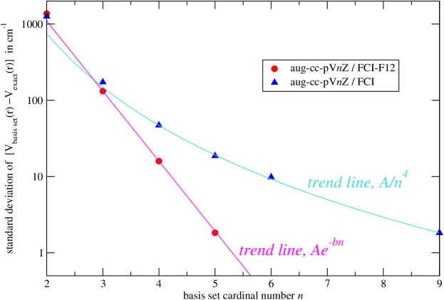
Figure 1: Convergence speed of H₂ relative energies with various basis sets. The quantity plotted is the standard deviation of the difference between a potential curve obtained with a given basis set and the virtually exact one from ref. Pachucki (2010) in the range $r=0.75$ a₀ to $r=12$ a₀. The trend lines are fits to the last three points of each series.

An analysis of the convergence pattern reveals that FCI errors decrease with the basis set cardinal number $n$ with an $n^{-4}$ dependence; for this reason the basis set extrapolation formula $E_{n}=E_{\infty}+A/n^{4}$ works best for this system and was used throughout. This observation is in line with several recent studies Peterson et al. (2012); Feller et al. (2011) which show very good performance for the similar formula $E_{n}=E_{\infty}+A/(n+1/2)^{4}$ with respect to other basis set extrapolation schemes. As a result of this regular convergence behaviour extrapolated a[5,6]z energy levels improve very significantly over the raw a6z values and have an accuracy comparable with the expected one for the a9z basis set. In particular, the error of a[5,6]z vibrational energy levels is very nearly linear up to $v=9$ and has an approximate magnitude of $0.12~{}v$ cm^-1. As discussed in detail below, similar basis set errors are found for H${}_{3}^{+}$.

Explicitly-correlated methods of the F12 type do exceptionally well for H₂ and show exponential convergence in terms of $n$ (see table 1 and fig. 1); as a result a5z/F12 energy levels are of overall higher quality than extrapolated a[56]z ones, especially for energies above 20 000 cm^-1. We also considered the basis sets of the cc-pV$n$Z-F12 family ($n=$ D, T and Q) Peterson et al. (2008); Yousaf and Peterson (2008) especially designed for F12 calculations; these basis sets too show exponential convergence and, moreover, reduce errors with respect to the corresponding a$n$z basis set by a factor 7 for a2z and by a factor 3 for a3z and a4z.

The first FCI calculations for H${}_{3}^{+}$  were performed in a classic 1986 work by Meyer, Botschwina and Burton (MBB) Meyer et al. (1986); subsequent studies gradually increased the accuracy of the PES and extended its range. Most of this work was performed ab initio  Lie and Frye (1992); Cencek et al. (1998); Polyansky et al. (2000); Bachorz et al. (2009); Pavanello et al. (2012a); Viegas et al. (2007); Velilla et al. (2008) but in a few cases the PES was improved by fitting to spectroscopic data Dinelli et al. (1994); Tennyson et al. (1995); Prosmiti et al. (1997); Pavanello et al. (2012a). These theoretical studies proved indispensable for the assignment of new observed lines of H${}_{3}^{+}$, see for example refs. Majewski et al. (1989); Lee et al. (1991); Dinelli et al. (1997); Asvany et al. (2007).

We performed FCI calculations at the 69 geometries originally used by MBB Meyer et al. (1986) for H${}_{3}^{+}$ using the same methodology described above for H₂; energies were fitted in a standard way, following the procedure described previously Polyansky and Tennyson (1999). These calculations are compared to the high-accuracy values computed by Cencek et al. Cencek et al. (1998) instead of the more recent and accurate one by Pavanello et al. Pavanello et al. (2012a, b) used elsewhere in this work because the latter were computed on a different grid. The results of Cencek et al. are sufficiently accurate for this purpose and will be labelled as ‘exact’ below. The results of the vibrational $J=0$ energy levels are reported in table 2. Explicitly correlated F12 methods show improved convergence speed but not quite as fast as for H₂; as a result extrapolated a[56]z and a5z-F12 energy levels have comparable accuracies (see table 2).

Table 2: Errors in H${}_{3}^{+}$ vibrational band origins ($J=0$) energy levels computed from FCI non-relativistic energy curves and various basis sets (see text for details). All values are in cm^-1.

$(v_{1},v_{2}^{\ell})$	exacta	exact - calculated
		a5z	a6z	a5z/F12	a[5,6]zb
$(0,1^{1})$	2 521.51	0.74	0.47	0.17	0.11
$(1,0^{0})$	3 179.59	0.44	0.35	0.07	0.16
$(0,2^{0})$	4 778.34	1.58	0.94	0.32	0.12
$(0,2^{2})$	4 998.31	1.52	0.92	0.32	0.14
$(1,1^{1})$	5 555.42	1.17	0.80	0.23	0.26
$(2,0^{0})$	6 264.44	0.90	0.66	0.13	0.30
$(0,3^{1})$	7 006.10	2.42	1.40	0.46	0.42
$(0,3^{3})$	7 285.50	2.52	1.43	0.44	0.44
$(1,2^{0})$	7 770.20	2.87	1.18	0.33	-0.09
$(1,2^{2})$	7 870.84	2.04	1.26	0.35	-0.00
$(2,1^{1})$	8 489.38	1.70	1.11	0.25	-0.03
$(0,4^{0})$	9 001.04	3.32	1.87	0.58	0.62
$(0,4^{2})$	9 112.17	3.44	1.90	0.56	0.74
$(3,0^{0})$	9 254.77	1.43	0.97	0.16	0.17
$(1,3^{1})$	9 653.33	3.00	1.75	0.45	-0.51
$(1,3^{3})$	9 966.80	2.91	1.68	0.16	-0.96
$(0,4^{4})$	9 997.51	2.54	1.58	0.36	-0.96
$(2,2^{0})$	10 592.76	2.15	1.37	0.11	-2.22
$(2,2^{2})$	10 643.45	2.31	1.46	0.02	-2.41
$(0,5^{1})$	10 855.91	3.83	1.90	-0.08	-0.18
RMSc=		2.33	1.33	0.32	0.85

^a Using the very accurate BO potential energy surface by Cencek et al Cencek et al. (1998).

^b Using extrapolation formula $E_{n}=E_{\infty}+A/n^{4}$.

^c Root-mean-square deviation in cm^-1.

Our FCI-based energy levels for H₂ have a root-mean-square (RMS) deviation with respect to the exact reference values of 1.66 cm^-1 (extrapolated a[56]z energies) or 0.47 cm^-1 (a5z-F12 energies); the RMS errors for H${}_{3}^{+}$ in the energy range to 10 000 cm^-1 are 0.85 cm^-1 (a[56]z) and 0.32 cm^-1 (a5z-F12). We conclude that F12 methods at the a5z level are capable of providing energy levels accurate to better than 0.5 cm^-1, and a[56]z generally to better than 1.5 cm^-1. Such calculations are therefore a viable, good-quality alternative when explicitly-correlated Gaussian methods are too expensive.

II.2 Relativistic surfaces

The most accurate relativistic corrections for H${}_{3}^{+}$ are those by Bachorz et al Bachorz et al. (2009) and were computed as expectation value (using a very accurate wave function based on explicitly correlated Gaussians) of the complete Breit-Pauli relativistic Hamiltonian Bethe and Salpeter (2008), i.e. including mass-velocity, one- and two-electron Darwin contributions, Breit retardation and spin-spin Fermi contact term. The relativistic correction for H${}_{3}^{+}$ is overall very small, spanning the range -4.3 to -1.8 cm^-1 over all the geometries considered. As discussed below such a small contribution is due to almost complete cancellation between the main contributions to the overall relativistic correction.

We used Molpro Werner et al. (2012) to compute relativistic corrections as expectation value of the mass-velocity (MV) and one-electron Darwin (D1) operator using full-CI wave functions. The Molpro-based aug-cc-pV6Z MVD1 energies are converged with respect to basis set to about 0.05 cm^-1; they typically agree with the more complete relativistic corrections by Bachorz to 0.15 cm^-1, which can only be considered a moderate agreement considering the overall smallness of the relativistic correction. This should indicate that the contribution to relative energies of terms neglected in the Molpro-based calculation (Breit, two-electron Darwin and Fermi contact) are non-negligible for very accurate work. On the other hand this also indicates that the two-electron QED correction (based on the two-electron Darwin contribution) should be negligible, as it is expected to be about 6 times smaller than the one-electron part.

It is worth performing a more detailed analysis of the MVD1 correction. The MV term has an absolute magnitude of about -23 cm^-1, while the D1 term of about +20 cm^-1; both contributions show a variation with geometry spanning about 6 cm^-1. However, the variation with geometry of MV and D1 are almost perfectly anti-correlated resulting in mutual cancellation when summed. As a result of this cancellation the MVD1 contribution turns out to be only slightly larger than the QED one (see section III).

The situation is somewhat similar for water (analysis performed for energies up to 40 000 cm^-1) Lodi and Tennyson (2010). The MV term is in absolute terms (average value) -57 000 cm^-1 with a variation of 500 cm^-1, and D1 +45 000 cm^-1 with a variation of 400 cm^-1. The MVD1 term has a magnitude of -11 500 cm^-1 with a variation of 140 cm^-1. The QED correction for water is 1 000 cm^-1 with a variation of 2 cm^-1. So in the case of water there still is considerable cancellation, but not as much as in H${}_{3}^{+}$.

III Quantum electrodynamics corrections for H₂ and H${}_{3}^{+}$

Pyykkö et al Pyykkö et al. (2001); Pyykkö (2012) proposed making use of approximate proportionality formulae between the leading QED corrections to order $\alpha^{3}$ (namely, the electron self-energy) and the one- and two-electron Darwin corrections. We neglect the two-electron contribution and compute the one-electron Darwin term with Molpro and FCI wavefunctions; as discussed in section II.2 the two-electron contribution is expected to be about a factor 6 smaller than the one-electron one. Pyykkö et al’s method requires a scaling factor for which we use 0.04669, as reported in table II of Pyykkö et al for all systems studied.

QED corrections are known accurately both for H${}_{2}^{+}$ Moss (1993) and H₂ Komasa et al. (2011); Salumbides et al. (2011); Dickenson et al. (2013); we compare our scheme with these reference calculations in tables 3 and 4.

The QED values differ on average from exact ones by less than 0.001 cm^-1 for H${}_{2}^{+}$ and less than 0.02 cm^-1 for H₂(see tables III and IV). Columns three and four of table 4 give the relativistic and QED shifts in the energy levels of H₂ from the exact calculations Komasa et al. (2011). Column 6 gives the relativistic FCI a[5,6]z calculation of MVD1 using Molpro and the column 7 gives the scaled by 0.04669 value of column 6, which gives our approximate QED value. One can see that the exact shifts differ from our approximate calculations by 0.02 cm^-1 or less for all except the highest, $v=14$ vibrational level. We express the substantiated hope here that the QED calculation for H${}_{3}^{+}$, given below, deviates from any future exact calculation by not much more than this value.

Let us now consider our analogous QED calculations for H${}_{3}^{+}$. The MVD1 calculations were also performed using Molpro and the a6z CBS basis set. However, our comparison of these calculations with one performed using a aQz basis set showed rapid convergence of the relativistic calculations with basis set, so in practice our aQz results could have been also used. Table  5 gives values for the calculated QED corrections at all 69 MBB geometries. It can be seen the magnitude of the QED correction is small, less than 1 cm^-1 everywhere, but that it varies significantly with geometry and even changes sign. We fitted the 69 QED points computed at the a6z level to the functional form used if ref. Pavanello et al. (2012a) to fit the relativistic energies. The function contained 9 fitting parameters, polynomials up to degree 4 and reproduced the ab initio values with a root-mean-square deviation of 3.3$\times$ 10^-3 cm^-1.

Table 3: QED corrections for $J=0$ vibrational levels of H${}_{2}^{+}$.

BO^a QED corrections exact^b this work exact – this work $v$ a4z a5z a6z a4z a5z a6z 0 0.00 0.000 0.000 0.000 0.000 0.000 0.000 0.000 1 2192.04 -0.009 -0.009 -0.009 -0.009 -0.001 0.000 0.000 2 4256.71 -0.018 -0.016 -0.017 -0.018 -0.001 -0.001 0.000 3 6198.28 -0.026 -0.024 -0.025 -0.025 -0.002 -0.001 0.000 4 8020.34 -0.033 -0.030 -0.032 -0.033 -0.003 -0.001 0.000 5 9725.84 -0.040 -0.036 -0.038 -0.039 -0.003 -0.001 0.000 6 11317.03 -0.046 -0.042 -0.044 -0.045 -0.003 -0.001 0.000 7 12795.56 -0.051 -0.047 -0.050 -0.051 -0.004 -0.001 0.000 8 14162.40 -0.056 -0.052 -0.055 -0.056 -0.004 -0.001 0.000 9 15417.90 -0.061 -0.056 -0.059 -0.061 -0.004 -0.001 0.000 10 16561.70 -0.065 -0.060 -0.063 -0.065 -0.005 -0.001 0.000 11 17592.67 -0.068 -0.063 -0.067 -0.068 -0.005 -0.001 0.000 12 18508.81 -0.072 -0.066 -0.070 -0.072 -0.005 -0.001 0.000 13 19307.16 -0.074 -0.069 -0.073 -0.074 -0.005 -0.001 0.000 14 19983.67 -0.076 -0.071 -0.075 -0.077 -0.005 -0.001 0.000 15 20533.04 -0.078 -0.073 -0.077 -0.078 -0.005 -0.001 0.000 16 20948.70 -0.079 -0.074 -0.078 -0.080 -0.005 -0.001 0.000 17 21223.28 -0.080 -0.075 -0.079 -0.081 -0.005 -0.001 0.001 18 21352.91 -0.080 -0.075 -0.079 -0.081 -0.005 -0.001 0.001 19 21375.30 -0.080 -0.075 -0.079 -0.081 -0.005 -0.001 0.001

^a Indicative non-relativististic Born-Oppenheimer values obtained with basis-set-extrapolated a[5,6]z energies; the extrapolation formula is $E_{n}=E_{\infty}+Ae^{-\alpha\sqrt{n}}$. Reported values have an estimated error of less than $0.10\times v$ cm^-1.

^b Taken from ref. Moss (1993).

^c This work, using the a5z

Table 4: QED corrections for H₂  for $J=0$ vibrational levels.

exact^b this work error^c $v$ BO^a $\alpha^{2}$ $\alpha^{3}$ total $\alpha^{2}$ $\alpha^{3}$ total total 0 0.00 0.00 0.00 0.00 0.00 0.00 0.00 -0.00 1 4,163.40 0.02 -0.02 0.00 0.03 -0.02 0.01 -0.01 2 8,091.16 0.04 -0.04 0.00 0.06 -0.04 0.01 -0.01 3 11,788.14 0.05 -0.06 -0.01 0.07 -0.06 0.01 -0.02 4 15,257.39 0.06 -0.08 -0.02 0.08 -0.08 0.00 -0.02 5 18,499.88 0.06 -0.09 -0.03 0.09 -0.10 -0.02 -0.02 6 21,514.30 0.05 -0.11 -0.05 0.08 -0.12 -0.04 -0.02 7 24,296.64 0.04 -0.12 -0.08 0.07 -0.13 -0.07 -0.02 8 26,839.64 0.02 -0.13 -0.12 0.04 -0.15 -0.10 -0.02 9 29,131.99 -0.02 -0.15 -0.16 0.01 -0.16 -0.15 -0.01 10 31,157.32 -0.06 -0.16 -0.22 -0.04 -0.17 -0.21 -0.01 11 32,892.55 -0.12 -0.17 -0.29 -0.10 -0.19 -0.29 -0.00 12 34,305.64 -0.20 -0.18 -0.37 -0.18 -0.20 -0.38 0.01 13 35,352.20 -0.29 -0.18 -0.48 -0.29 -0.21 -0.50 0.02 14 35,970.80 -0.42 -0.19 -0.61 -0.43 -0.22 -0.65 0.04

^a Using the very accurate BO potential energy points by Pachucki Pachucki (2010).

^b From Komasa et al. Komasa et al. (2011); corrections to order $\alpha^{4}$ were also estimated in ref. Komasa et al. (2011) but contribute by less than 0.002 cm^-1 for all energy levels.

^c exact - this work

Table 5: QED corrections, $\Delta V_{\rm QED}$ in cm^-1, computed at the 69 MBB geometries Meyer et al. (1986) using a Molpro and an a5z FCI wavefunction..

na	nx	ny	$\Delta V_{\rm QED}$		na	nx	ny	$\Delta V_{\rm QED}$
-4	0	0	0.5588		1	-1	0	-0.0890
-3	0	0	0.3879		1	-2	0	-0.0611
-2	0	0	0.2403		1	-3	0	-0.0126
-1	0	0	0.1121		1	-4	0	0.0594
0	0	0	0.0000		2	-1	0	-0.1749
1	0	0	-0.0981		2	-2	0	-0.1482
2	0	0	-0.1838		2	-3	0	-0.1022
3	0	0	-0.2580		2	-4	0	-0.0345
4	0	0	-0.3217		3	-1	0	-0.2494
5	0	0	-0.3750		3	-2	0	-0.2236
0	-1	0	0.0095		3	-3	0	-0.1797
0	-2	0	0.0391		3	-4	0	-0.1152
0	-3	0	0.0910		4	-1	0	-0.3133
0	-4	0	0.1677		4	-2	0	-0.2883
-1	-1	0	0.1223		4	-3	0	-0.2461
-1	-2	0	0.1542		5	-1	0	-0.3668
-1	-3	0	0.2101		1	1	0	-0.0891
-2	-1	0	0.2515		1	2	0	-0.0624
-2	-2	0	0.2863		1	3	0	-0.0178
-2	-3	0	0.3466		2	1	0	-0.1750
-3	-1	0	0.4002		2	2	0	-0.1485
-3	-2	0	0.4380		2	3	0	-0.1032
-4	-1	0	0.5719		3	1	0	-0.2493
0	1	0	0.0093		3	2	0	-0.2225
0	2	0	0.0366		4	1	0	-0.3129
0	3	0	0.0820		4	2	0	-0.2847
-1	1	0	0.1218		5	1	0	-0.3658
-1	2	0	0.1504		0	0	2	0.0378
-1	3	0	0.1977		-2	0	2	0.2839
-2	1	0	0.2508		-2	0	3	0.3393
-2	2	0	0.2815		0	0	3	0.0864
-2	3	0	0.3319		0	0	4	0.1568
-3	1	0	0.3995		2	0	2	-0.1483
-3	2	0	0.4328		2	0	3	-0.1032
-4	1	0	0.5713

IV Rovibrational calculations for H${}_{3}^{+}$  with the QED surface

We used the DVR3D program suite Tennyson et al. (2004) to compute ro-vibrational energy levels using the same parameters employed in previous studies Pavanello et al. (2012a, b); energy levels are converged with respect to the nuclear motion problem to 0.001 cm^-1. Nuclear motion calculations used the new, accurate, global GLH3P PES of Pavanello et al. Pavanello et al. (2012a). This is the most accurate PES available for H${}_{3}^{+}$ and includes a non-relativistic BO component computed using explicitly correlated Gaussian functions Pavanello et al. (2012a, b); Pavanello et al. (2009), an adiabatic Born-Oppenheimer diagonal correction (BODC) surface Pavanello et al. (2012a) and a relativistic surface Pavanello et al. (2012a, b). The BO, adiabatic and relativistic surfaces are supposed to be accurate to about $10^{-2}$ cm^-1Pavanello et al. (2012a, b). Here we combine our QED surface with the other surfaces used previously Pavanello et al. (2012a). Calculations were performed without and with allowance for non-nadiabatic effects; results are collected in table 6.

Table 6: Vibrational band origins ($J=0$ energy levels) for H${}_{3}^{+}$ calculated with various models of non-adiabatic effects and with or without QED corrections. All values are in cm^-1.

non-ad.a=		nuc	nuc	PT	PT	Din	Din
QEDb=		no	yes	no	yes	no	yes
$(v_{1},v_{2}^{\ell})$	obs.c	obs.-calc.
(0,11)	2521.41	-0.18	-0.14	0.11	0.16	0.01	0.05
(0,22)	4998.04	-0.42	-0.33	0.14	0.23	-0.03	0.05
(1,11)	5554.06	-0.78	-0.71	-0.14	-0.07	-0.35	-0.28
(0,33)	7492.91	-0.74	-0.61	0.13	0.26	-0.15	-0.03
(0,42)	9113.08	-0.88	-0.73	0.04	0.19	-0.26	-0.11
(2,22)	10645.38	-1.05	-0.95	0.06	0.20	-0.30	-0.16
(0,51)	10862.91	-0.85	-0.66	0.16	0.34	-0.18	0.00
(3,11)	11323.10	-1.27	-1.14	-0.02	0.11	-0.41	-0.29
(0,55)	11658.40	-1.08	-0.90	0.09	0.27	-0.28	-0.10
(2,31)	12303.37	-1.15	-0.95	0.03	0.22	-0.35	-0.16
(0,62)	12477.38	-1.18	-0.98	-0.02	0.18	-0.39	-0.19
(0,71)	13702.38	-1.33	-1.12	-0.21	0.00	-0.62	-0.41
(0,82)	15122.81	-1.28	-1.06	0.16	0.38	-0.39	-0.18
RMSd		0.99	0.84	0.12	0.22	0.33	0.19

^a Treatment used for non-adiabatic effects. ‘nuc’ indicates nuclear masses were used (i.e., no allowance made for non-adiabatic effects). ‘PT’ indicated the Polyansky-Tennyson model Polyansky and Tennyson (1999) with constant effective rotational and vibrational masses. ‘Din’ is the model by Diniz et al. Diniz et al. (2013)

^b Indicates whether the QED correction surface was included or not.

^c Experimentally-derived energy levels, from Furthenbacher et al. Furtenbacher et al. (2013b).

^d Root-mean-square deviation.

Without inclusion of QED effects, the RMS deviation obtained for the vibrational band origins below 16 000 cm^-1 is 0.99 cm^-1 using nuclear masses and no allowance for non-adiabatic effects; inclusion of QED effects results in a reduction of the RMS deviation to 0.84 cm^-1. The effect of QED is therefore much larger than the desired accuracy of $10^{-2}$ cm^-1  for H${}_{3}^{+}$. The resulting observed $-$ calculated residues can be ascribed almost completely to non-adiabatic effects.

To further increase the accuracy non-adiabatic effects have to be taken into account; at the moment this can be done only in an approximate way, for example using effective rotational and vibrational masses (PT model Polyansky and Tennyson (1999)) or using the more refined model by Diniz et al Diniz et al. (2013).

To extend the Diniz et al model to higher vibrational states we first calculated $J=0$ energies and wavefunctions, $\Psi_{n}$, using nuclear masses. We used these wavefunctions and the mass surface, $m(\underline{R})$, given by Diniz et al to obtain an improved, effective mass, $m_{n}$, for each vibrational state $n$ computed as $m_{n}=\langle\Psi_{n}|m(\underline{R})|\Psi_{n}\rangle>$. Energies for $J=0$ were then recalculated for each vibrational state in turn using the improved (constant) state-dependent mass.

Calculations with a vibrational mass of 1.0007537 u using the PT model results in a RMS deviation of 0.12 cm^-1, see table 6. Inclusion of QED degrades the RMS deviation to 0.22 cm^-1 in this model. On the other hand in the more refined model of Diniz et al.  Diniz et al. (2013) for non-adiabatic effects inclusion of QED effects leads to a reduction of the RMS deviation from 0.33 cm^-1 without QED effects to 0.19 cm^-1 when QED is included.

Table 6 therefore demonstrates that further work is needed to improve non-adiabatic models as well as that QED corrections are indispensable to any calculations which include non-adiabatic corrections in order to approach observed values.

V Conclusions

We calculated a QED energy correction surface for H${}_{3}^{+}$ using the approximate method of Pyykkö et al. Pyykkö et al. (2001). This method is benchmarked against accurate QED calculations for H${}_{2}^{+}$ and H₂; the comparisons suggest that our QED surface for H${}_{3}^{+}$ should provide QED corrections to rotational-vibration energy levels with an accuracy better than $0.02$ cm^-1. The effect of QED on low-lying energy levels is of the order of 0.2 cm^-1 and hence is much larger than the accuracy of $10^{-2}$ cm^-1 which has already been achieved for all components of ab initio  calculations on H${}_{3}^{+}$ with the notable exception of non-adiabatic effects.

Inclusion of QED effects leads to H${}_{3}^{+}$ energy levels being reproduced with a RMS deviation which is reduced from 0.99 cm^-1  to 0.84 cm^-1 when no allowance is made for non-adiabatic effects (nuclear masses used for energy levels calculation). These calculations, which include highly accurate BO, adiabatic, relativistic and QED effects but no provision for non-adiabatic effects, therefore represent an accurate characterisation of the value of non-adiabatic effects for each H${}_{3}^{+}$ level. Allowance for non-adiabatic effects using the simple model of PT Polyansky and Tennyson (1999) results in a further reduction of this deviation to 0.22 cm^-1. Use of the non-adiabatic model of Diniz et al. shows that in this model the use of QED corrections reduces the errors in the results by almost a factor of two from 0.33 cm^-1 to 0.19 cm^-1. This demonstrates the necessity of including QED corrections in accurate ab initio treatments of H${}_{3}^{+}$ rotation-vibration energy levels; it opens the way for the development of an accurate non-adiabatic model which could potentially reach the $10^{-2}$ cm^-1  accuracy necessary for the assignment of Carrington – Kennedy Carrington et al. (1982) near-dissociation spectrum of H${}_{3}^{+}$ and its isotopologues.

References

- Pyykkö (2012) P. Pyykkö, Chem. Rev. 112, 371 (2012).
- Liu (2014) W. Liu, Phys. Rep. (2014), (in press).
- Autschbach (2012) J. Autschbach, J. Chem. Phys. 136, 150902 (2012).
- Liu (2012) W. Liu, Phys. Chem. Chem Phys. 14, 35 (2012).
- Kutzelnigg (2012) W. Kutzelnigg, Chem. Phys. 395, 16 (2012).
- Iliaš et al. (2010) M. Iliaš, V. Kellö, and M. Urban, Acta Physica Slovaca 60, 259 (2010).
- Tarczay et al. (2001) G. Tarczay, A. G. Császár, W. Klopper, and H. M. Quiney, Mol. Phys. 99, 1768 (2001).
- Reiher and Wolf (2009) M. Reiher and A. Wolf, Relativistic Quantum Chemistry (Wiley, 2009).
- Dyall and Faegri (2007) K. G. Dyall and K. Faegri, Introduction to Relativistic Quantum Chemistry (Oxford University Press, 2007).
- Moss (1999) R. E. Moss, J. Phys. B: At. Mol. Opt. Phys. 32, L89 (1999).
- Korobov (2006) V. I. Korobov, Phys. Rev. A 74, 052506 (2006).
- Korobov (2008) V. I. Korobov, Phys. Rev. A 77, 022509 (2008).
- Zhong et al. (2012) Z.-X. Zhong, P.-P. Zhang, Z.-C. Yan, and T.-Y. Shi, Phys. Rev. A 86, 064502 (2012).
- Komasa et al. (2011) J. Komasa, K. Piszczatowski, G. Łach, M. Przybytek, B. Jeziorski, and K. Pachucki, J. Chem. Theor. Comp. 7, 3105 (2011).
- Salumbides et al. (2011) E. J. Salumbides, G. D. Dickenson, T. I. Ivanov, and W. Ubachs, Phys. Rev. Lett. 107, 043005 (2011).
- Dickenson et al. (2013) G. D. Dickenson, M. L. Niu, E. J. Salumbides, J. Komasa, K. S. E. Eikema, K. Pachucki, and W. Ubachs, Phys. Rev. Lett 110, 193601 (2013).
- Pavanello et al. (2012a) M. Pavanello, L. Adamowicz, A. Alijah, N. F. Zobov, I. I. Mizus, O. L. Polyansky, J. Tennyson, T. Szidarovszky, A. G. Császár, M. Berg, et al., Phys. Rev. Lett. 108, 023002 (2012a).
- Carrington et al. (1982) A. Carrington, J. Buttenshaw, and R. A. Kenedy, Mol. Phys. 45, 753 (1982).
- Carrington and Kennedy (1984) A. Carrington and R. A. Kennedy, J. Chem. Phys. 81, 91 (1984).
- Carrington and McNab (1989) A. Carrington and I. R. McNab, Acc. Chem. Res. 22, 218 (1989).
- Tennyson (1995) J. Tennyson, Rep. Prog. Phys. 58, 421 (1995).
- Wu et al. (2013) K.-Y. Wu, Y.-H. Lien, C.-C. Liao, Y.-R. Lin, and J.-T. Shy, Phys. Rev. A 88, 032507 (2013).
- Hodges et al. (2013) J. N. Hodges, A. J. Perry, P. A. Jenkins, B. M. Siller, and B. J. McCall, J. Chem. Phys. 139, 164201 (2013).
- Furtenbacher et al. (2007) T. Furtenbacher, A. G. Császár, and J. Tennyson, J. Mol. Spectrosc. 245, 115 (2007).
- Furtenbacher et al. (2013a) T. Furtenbacher, T. Szidarovszky, C. Fábri, and A. G. Császár, Phys. Chem. Chem. Phys. 15, 10181 (2013a).
- Furtenbacher et al. (2013b) T. Furtenbacher, T. Szidarovszky, E. Mátyus, C. Fábri, and A. G. Császár, J. Chem. Theory Comput. 9, 5471 (2013b).
- Pavanello et al. (2012b) M. Pavanello, L. Adamowicz, A. Alijah, N. F. Zobov, I. I. Mizus, O. L. Polyansky, J. Tennyson, T. Szidarovszky, and A. G. Császár, J. Chem. Phys. 136, 184303 (2012b).
- Polyansky and Tennyson (1999) O. L. Polyansky and J. Tennyson, J. Chem. Phys. 110, 5056 (1999).
- Moss (1993) R. E. Moss, Mol. Phys 80, 1541 (1993).
- Diniz et al. (2013) L. G. Diniz, J. R. Mohallem, A. Alijah, M. Pavanello, L. Adamowicz, O. L. Polyansky, and J. Tennyson, Phys. Rev. A 88, 032506 (2013).
- Polyansky et al. (2003) O. L. Polyansky, A. G. Császár, S. V. Shirin, N. F. Zobov, P. Barletta, J. Tennyson, D. W. Schwenke, and P. J. Knowles, Science 299, 539 (2003).
- Polyansky et al. (2013) O. L. Polyansky, R. I. Ovsyannikov, A. A. Kyuberis, L. Lodi, J. Tennyson, and N. F. Zobov, J. Phys. Chem. A 117, 9633–9643 (2013).
- Boyarkin et al. (2013) O. V. Boyarkin, M. A. Koshelev, O. Aseev, P. Maksyutenko, T. R. Rizzo, N. F. Zobov, L. Lodi, J. Tennyson, and O. L. Polyansky, Chem. Phys. Lett. 568-–569, 14 (2013).
- Werner et al. (2012) H.-J. Werner, P. J. Knowles, G. Knizia, F. R. Manby, M. Schütz, et al., Molpro, version 2012.1, a package of ab initio programs (2012), ”see http://www.molpro.net”.
- Dunning, Jr (1989) T. H. Dunning, Jr, J. Chem. Phys. 90, 1007 (1989).
- Shiozaki and Werner (2013) T. Shiozaki and H.-J. Werner, Mol. Phys. 111, 607 (2013).
- Hättig et al. (2012) C. Hättig, W. Klopper, A. Köhn, and D. P. Tew, Chem. Rev. 112, 4 (2012).
- Kong et al. (2012) L. Kong, F. A. Bischoff, and E. F. Valeev, Chem. Rev. 112, 75 (2012).
- Ten-No and Noga (2012) S. Ten-No and J. Noga, WIREs Comput. Mol. Sci. 2, 114 (2012).
- Shiozaki et al. (2011) T. Shiozaki, G. Knizia, and H.-J. Werner, J. Chem. Phys. 134, 034113 (2011).
- Pachucki (2012) K. Pachucki, Phys. Rev. A 85, 042511 (2012).
- Pachucki (2010) K. Pachucki, Phys. Rev. A 82, 032509 (2010).
- Peterson et al. (2012) K. A. Peterson, D. Feller, and D. A. Dixon, Theor. Chem. Acc. 131, 1079 (2012).
- Feller et al. (2011) D. Feller, K. A. Peterson, and J. G. Hill, J. Chem. Phys. 135, 044102 (2011).
- Peterson et al. (2008) K. A. Peterson, T. B. Adler, and H.-J. Werner, J. Chem. Phys. 128, 084102 (2008).
- Yousaf and Peterson (2008) K. E. Yousaf and K. A. Peterson, J. Chem. Phys. 129, 184108 (2008).
- Meyer et al. (1986) W. Meyer, P. Botschwina, and P. R. Burton, J. Chem. Phys. 84, 891 (1986).
- Lie and Frye (1992) G. C. Lie and D. Frye, J. Chem. Phys. 96, 6784 (1992).
- Cencek et al. (1998) W. Cencek, J. Rychlewski, R. Jaquet, and W. Kutzelnigg, J. Chem. Phys. 108, 2831 (1998).
- Polyansky et al. (2000) O. L. Polyansky, R. Prosmiti, W. Klopper, and J. Tennyson, Mol. Phys. 98, 261 (2000).
- Bachorz et al. (2009) R. A. Bachorz, W. Cencek, R. Jaquet, and J. Komasa, J. Chem. Phys. 131, 024105 (2009).
- Viegas et al. (2007) L. P. Viegas, A. Alijah, and A. J. C. Varandas, J. Chem. Phys. 126, 074309 (2007).
- Velilla et al. (2008) L. Velilla, B. Lepetit, A. Aguado, J. A. Beswick, and M. Paniagua, J. Chem. Phys. 129, 084307 (2008).
- Dinelli et al. (1994) B. M. Dinelli, S. Miller, and J. Tennyson, J. Mol. Spectrosc. 163, 71 (1994).
- Tennyson et al. (1995) J. Tennyson, B. M. Dinelli, and O. L. Polyansky, J. Molec. Struct. (THEOCHEM) 341, 133 (1995).
- Prosmiti et al. (1997) R. Prosmiti, O. L. Polyansky, and J. Tennyson, Chem. Phys. Lett. 273, 107 (1997).
- Majewski et al. (1989) W. A. Majewski, P. A. Feldman, J. K. G. Watson, S. Miller, and J. Tennyson, Astrophys. J. 347, L51 (1989).
- Lee et al. (1991) S. S. Lee, B. F. Ventrudo, D. T. Cassidy, T. Oka, S. Miller, and J. Tennyson, J. Mol. Spectrosc. 145, 222 (1991).
- Dinelli et al. (1997) B. M. Dinelli, L. Neale, O. L. Polyansky, and J. Tennyson, J. Mol. Spectrosc. 181, 142 (1997).
- Asvany et al. (2007) O. Asvany, E. Hugo, S. Schlemmer, F. Muller, F. Kuhnemann, S. Schiller, and J. Tennyson, J. Chem. Phys. 127, 154317 (2007).
- Bethe and Salpeter (2008) H. A. Bethe and E. E. Salpeter, Quantum Mechanics of one- and two-electron systems (Dover Publications, 2008), originally published by Academic Press, 1957.
- Lodi and Tennyson (2010) L. Lodi and J. Tennyson, J. Phys. B: At. Mol. Opt. Phys. 43, 133001 (2010).
- Pyykkö et al. (2001) P. Pyykkö, K. G. Dyall, A. G. Császár, G. Tarczay, O. L. Polyansky, and J. Tennyson, Phys. Rev. A 63, 024502 (2001).
- Tennyson et al. (2004) J. Tennyson, M. A. Kostin, P. Barletta, G. J. Harris, O. L. Polyansky, J. Ramanlal, and N. F. Zobov, Comput. Phys. Commun. 163, 85 (2004).
- Pavanello et al. (2009) M. Pavanello, W.-C. Tung, F. Leonarski, and L. Adamowicz, J. Chem. Phys. 130, 074105 (2009).