MAD Bayes for Tumor Heterogeneity – Feature Allocation with Exponential Family Sampling

Abstract

We propose small-variance asymptotic approximations for inference on tumor heterogeneity (TH) using next-generation sequencing data. Understanding TH is an important and open research problem in biology. The lack of appropriate statistical inference is a critical gap in existing methods that the proposed approach aims to fill. We build on a hierarchical model with an exponential family likelihood and a feature allocation prior. The proposed implementation of posterior inference generalizes similar small-variance approximations proposed by Kulis and Jordan (2012) and Broderick et.al (2012b) for inference with Dirichlet process mixture and Indian buffet process prior models under normal sampling. We show that the new algorithm can successfully recover latent structures of different haplotypes and subclones and is magnitudes faster than available Markov chain Monte Carlo samplers. The latter are practically infeasible for high-dimensional genomics data. The proposed approach is scalable, easy to implement and benefits from the flexibility of Bayesian nonparametric models. More importantly, it provides a useful tool for applied scientists to estimate cell subtypes in tumor samples. R code is available on http://www.ma.utexas.edu/users/yxu/.

KEY WORDS: Bayesian nonparametric; Bregman divergence; Feature allocation; Indian buffet process; Next-generation sequencing; Tumor heterogeneity.

1 Introduction

1.1 MAD-Bayes

We propose a generalization of the MAD (maximum a posteriori based asymptotic derivations) Bayes approach of Broderick et al., 2012b to latent feature models beyond the conjugate normal-normal setup. The model is developed for inference on tumor heterogeneity (TH), when the sampling model is a binomial distribution for observed short reads counts for single nucleotide variants (SNVs) in next-generation sequencing (NGS) experiments.

The proposed model includes a Bayesian non-parametric (BNP) prior. BNP models are characterized by parameters that live on an infinite-dimensional parameter space, such as unknown mean functions or unknown probability measures. Related methods are widely used in a variety of machine learning and biomedical research problems, including clustering, regression and feature allocation. While BNP methods are flexible from a modeling perspective, a major limitation is the computational challenge that arises in posterior inference with large-scale problems and big data. Posterior inference in highly structured models is often implemented by Markov chain Monte Carlo (MCMC) simulation (Liu, , 2008, for example) or variational inference such as expectation-maximization (EM) algorithm (Dempster et al., , 1977). However, neither approach scales effectively to high-dimensional data. As a result, simple ad-hoc methods, such as K-means (Hartigan and Wong, , 1979), are still preferred in many large-scale applications. K-means clustering is often preferred over full posterior inference in model-based clustering, such as Dirichlet process (DP) mixture models. DP mixture models are some of the most widely used BNP models. See, for example, Ghoshal, (2010), for a review.

Despite the simplicity and scalability, K-means has some known shortcomings. First, the K-means algorithm is a rule-based method. The output is an ad-hoc point estimate of the unknown partition. There is no notion of characterizing uncertainty, and it is difficult to coherently embed it in a larger model. Second, the K-means algorithm requires a fixed number of clusters, which is not available in many applications. An ideal algorithm should combine the scalability of K-means with the flexibility of Bayesian nonparametric models. Such links between non-probabilistic (i.e., rule-based methods like K-means) and probabilistic approaches (e.g., posterior MCMC or the EM algorithm) can sometimes be found by using small-variance asymptotics. For example, the EM algorithm for a mixture of Gaussian model becomes the K-means algorithm as the variances of the Gaussians tend to zero (Hastie et al., , 2001). In general, small-variance asymptotics can offer useful alternative approximate implementations of inference for large-scale Bayesian nonparametric models, exploiting the fact that corresponding non-probabilistic models show advantageous scaling properties.

Using small-variance asymptotics, Kulis and Jordan, (2011) showed how a K-means-like algorithm could approximate posterior inference for Dirichlet process (DP) mixtures. Broderick et al., 2012b generalized the approach by developing small-variance asymptotics to MAP (maximum a posteriori) estimation in feature allocation models with Indian buffet process (IBP) priors (Griffiths and Ghahramani, , 2006; Teh et al., , 2007). Similar to the K-means algorithm, they proposed the BP (beta process)-means algorithm for feature learning. Both approaches are restricted to normal sampling and conjugate normal priors, which facilitates the asymptotic argument and greatly simplifies the computation. However, it is not immediately generalizable to other distributions, preventing their methodology from being applied to non-Gaussian data. The application that motivates the current paper is a typical example. We require posterior inference for a feature allocation model with a binomial sampling model.

1.2 Tumor Heterogeneity

The proposed methods are motivated by an application to inference for tumor heterogeneity (TH). This is a highly important and open research problem that is currently studied by many cancer researchers (Gerlinger et al., , 2012; Landau et al., , 2013; Larson and Fridley, , 2013; Andor et al., , 2014; Roth et al., , 2014). In the literature over the past five years a consensus has emerged that tumor cells are heterogenous, both within the same biological tissue sample and between different samples. A tumor sample typically comprises an admixture of subtypes of different cells, each possessing a unique genome. We will use the term “subclones” to refer to cell subtypes in a biological sample. Inference on genotypic differences (differences in DNA base pairs) between subclones and proportions of each subclone in a sample can provide critical new information for cancer diagnosis and prognosis. However, inference and statistical modeling are challenging and few solutions exist.

Genotypic differences between subclones do not occur frequently. They are often restricted to single nucleotide variations (SNVs). When a sample is heterogeneous, it contains multiple subclones with each subclone possessing a unique genome. Often the differences between subclonal genomes are marked by somatically acquired SNVs. For multiple samples from the same tumor, intra-tumor heterogeneity refers to the presence of multiple subclones that appear in different proportions across different samples. For samples from different patients, however, subclonal genomes are rarely shared due to polymorphism between patients. However, for a selected set of potentially disease related SNVs (e.g., from biomarker genes), one may still find locally shared haplotypes (a set of SNVs on the same chromosome) across patients consisting of the selected SNVs. Importantly, in the upcoming discussion we regard two subclonal genomes the same if they possess identical genotypes on the selected SNVs, regardless of the rest of genome. In other words, we do not insist that the whole genomes of any two cells must be identical in order to call them subclonal. Figure 1(a) illustrates how such different subclones can develop over the life history of a tumor, ending, in this illustration, with three subclones and five unique haplotypes (ACG, GGG, CGG, TGG, AGG).

We start with models for haplotypes. Having more than two haplotypes in a sample implies cellular heterogeneity.

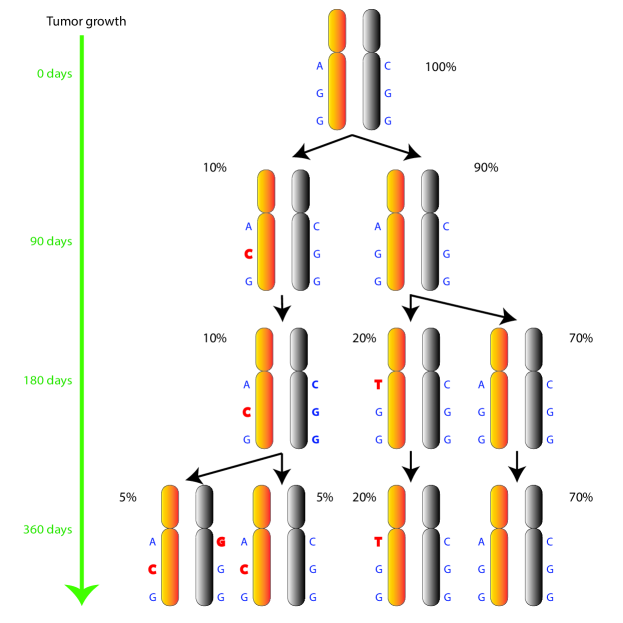
(a)

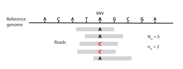
(b)

Figure 1: (a) Somatic mutations (in red) that are acquired during tumor growth lead to the emergence of new subclones and haplotypes. (b) An illustration of an SNV and read mapping. The figure shows five short reads that are mapped to the indicated SNV location. The reference genotype is A. Among the five reads, two reads have a variant genotype C. So $N_{st}=5$, $n_{st}=2$ and the observed VAF is $2/5$.

We use NGS data that record for each sample $t$ the number $N_{st}$ of short reads that are mapped to the genomic location of each of the selected SNVs $s$, $s=1,\ldots,S$. Some of these overlapping reads possess a variant sequence, while others include the reference sequence. Let $n_{st}$ denote the number of variant reads among the $N_{st}$ overlapping reads for each sample and SNV. In Figure 1(b), $N_{st}=5$ reads are mapped to the indicated SNV. While the reference sequence is “A”, $n_{st}=2$ short reads bear a variant sequence “C”. We define variant allele fraction (VAF) as the proportion $n_{st}/N_{st}$ of short reads bearing a variant genotype among all the short reads that are mapped to an SNV. In Figure 1(b), the VAF is 2/5 for that SNV. In Section 2, we will model the observed variant read counts by a mixture of latent haplotypes, which in turn are defined by a pattern of present and absent SNVs. Assuming that each sample is composed of some proportions of these haplotypes, we can then fit the observed VAFs across SNVs in each sample. Formally, modeling involves binomial sampling models for the observed counts with mixture priors for the binomial success probabilities. The mixture is over an (unknown) number $C$ of (latent) haplotypes, which in turn are represented as a binary matrix $\bm{Z}$, with columns, $c=1,\ldots,C,$ corresponding to haplotypes and rows, $s=1,\ldots,S$, corresponding to SNVs. The entries $z_{sc}\in\{0,1\}$ are indicators for variant allele $s$ appearing in haplotype $c$. That is, each column of indicators defines a haplotype by specifying the genotypes (variant or not) of the corresponding SNVs.

1.3 Main Contributions

A key element of the proposed model is the prior on the binary matrix $\bm{Z}$. We recognize the problem as a special case of a feature allocation problem and use an Indian buffet process (IBP) prior for $\bm{Z}$. In the language of feature allocation models (and the traditional metaphor that is used to describe the IBP prior), the haplotypes are the features (or dishes) and the SNVs are experimental units (or customers) that select features. Each tumor sample consists of an unknown proportion of these haplotypes. Lee et al., (2013) used a finite feature allocation model to describe the latent structure of possible haplotypes. The model is restricted to a fixed number of haplotypes. In practice, the number of haplotypes is unknown. A possible way to generalize to an unknown number of latent features is to define a transdimensional MCMC scheme, such as a reversible jump (RJ) algorithm (Green, , 1995). However, it is difficult to implement a practicable RJ algorithm.

An attractive alternative is to generalize the BP-means algorithm of Broderick et al., 2012b beyond the Gaussian case. Inspired by the connection between Bregman divergences (Bregman, , 1967) and exponential families, we propose a MAP-based small-variance asymptotic approximation for any exponential family likelihood with an IBP feature allocation prior. We call the proposed approach the FL-means algorithm, where FL stands for “feature learning”. The FL-means algorithm is scalable, easy to implement and benefits from the flexibility of Bayesian nonparametric models. Computation time is reduced beyond a factor 1,000.

This paper proceeds as follows. In Section 2, we introduce the Bayesian feature allocation model to describe tumor heterogeneity. Section 3 elaborates the FL-means algorithm and proves convergence. We examine the performance of FL-means through simulation studies in Section 4. In Section 5, we apply the FL-means algorithm to inference for TH. Finally, we conclude with a brief discussion in Section 6.

2 A Model for Tumor Heterogeneity

2.1 Likelihood

We consider data sets from NGS experiments. The data sets record the observed read counts for $S$ SNVs in $T$ tumor samples. Let $\bm{n}$ and $\bm{N}$ denote $S\times T$ matrices with $N_{st}$ denoting the total number of reads overlapping with SNV $s$ in tissue sample $t$, and $n_{st}$ denoting the number of variant reads among those $N_{st}$ reads. The ratio $n_{st}/N_{st}$ is the observed VAF. Figure 1(b) provides an illustration. We assume a binomial sampling model

$$p(n_{st}\mid N_{st},p_{st})=\mbox{Bin}(N_{st},p_{st}),$$

where $p_{st}$ is the expected VAF, $p_{st}=E(n_{st}/N_{st}\mid N_{st},p_{st})$. Conditional on $N_{st}$ and $p_{st}$, the observed counts $n_{st}$ are independent across $s$ and $t$. The likelihood becomes

$$p(\bm{n}\mid\bm{N},\bm{p})=\prod_{s=1}^{S}\prod_{t=1}^{T}{N_{st}\choose n_{st}}p_{st}^{n_{st}}(1-p_{st})^{(N_{st}-n_{st})},$$ (1)

where $\bm{n}=[n_{st}]$, $\bm{N}=[N_{st}]$ and $\bm{p}=[p_{st}]$ are $(S\times T)$ matrices. The binomial success probabilities $p_{st}$ are modeled in terms of latent haplotypes which we introduce next.

2.2 Prior Model for Haplotypes

Recall that $\{z_{sc}=1\}$ indicates that the genotype at SNV $s$ is a variant (different from the reference genotype) for haplotype $c$. Figure 2 illustrates the binary latent matrix $\bm{Z}=[z_{sc}]$ with $C=4$ haplotypes (columns) and $S=8$ SNVs (rows). A shaded cell indicates $z_{sc}=1$. For instance, SNV 2 occurs in two haplotypes $c=1$ and 3, SNV 3 occurs only in haplotype $c=3$.

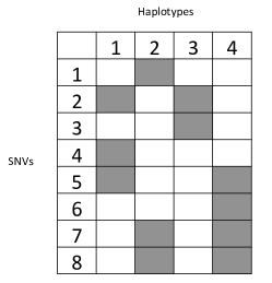
Figure 2: A binary matrix $\bm{Z}$ with haplotypes (latent features) $c=1,\ldots,C(=4)$, in the columns and $S=8$ SNVs in the rows. A shaded cell indicates that an SNV occurs in a haplotype ($z_{sc}=1$).

Assuming that each sample is composed of proportions $w_{tc}$ of the haplotypes, $c=1,\ldots,C$, we represent $p_{st}$ as

$$p_{st}=w_{t0}p_{0}+\sum_{c=1}^{C}w_{tc}z_{sc},$$ (2)

where $w_{tc}\in[0,1)$ and $\sum_{c=0}^{C}w_{tc}=1$.

In (2), we introduce an additional background haplotype $c=0$ that captures experimental and data processing noise, such as the fraction of variant reads that are mapped with low quality or error. In the decomposition, $p_{0}$ is the relative frequency of an SNV in the background. Equation (2) is a key model assumption. It allows us to deduce the unknown haplotypes from a decomposition of the expected VAF $p_{st}$ as a weighted sum of latent genotype calls $z_{sc}$ with weights being the proportions of haplotypes. Importantly, we assume these weights to be the same across all SNVs, $s=1,\ldots,S$. In other words, the expected VAF is contributed by those haplotypes with variant genotypes, weighted by the haplotype prevalences. Haplotypes without variant genotype on SNV $s$ do not contribute to the VAF for $s$ since all the short reads generated from those haplotypes are normal reads. For example, in Figure 2 the variant reads mapped to SNV 2 should come from haplotypes 1 and 3, but not from 2 or 4.

The next step in the model construction is the prior model $p(\bm{Z}$). We use the IBP prior. See, for example Griffiths and Ghahramani, (2006), Thibaux and Jordan, (2007) or Teh et al., (2007) for a discussion of the IBP and for a generative model. We briefly review the construction in the context of the current application. We build the binary matrix $\bm{Z}$ one line (SNV) at a time, adding columns (haplotypes) when the first SNV appears with $z_{sc}=1$. Let $C_{s}$ denote the number of columns that are constructed by the first $s$ SNVs. For each SNV, $s=1,\ldots,S$, we introduce $C_{s}^{+}\sim\mbox{Poi}(\gamma/s)$ new haplotypes, and assign $z_{sc}=1$ and $z_{s^{\prime},c}=0,\forall s^{\prime}<s$, for the new haplotypes $c=C_{s-1}+1,\ldots,C_{s-1}+C_{s}^{+}=C_{s}.$ For the earlier haplotypes, $c=1,\ldots,C_{s-1}$, mutation $s$ is included with probability $p(z_{sc}=1)=\frac{m_{sc}}{s}$ (note the $s$, rather than $s-1$ in the denominator), where $m_{sc}=\sum_{s^{\prime}<s}z_{s^{\prime}c}$ denote the column sums up to row $s-1$, that is, the number of SNVs, $s^{\prime}<s$, that defines haplotype $c$. Implicit in the construction is a convention of indexing columns by order of appearance, that is, as columns are added for SNVs, $s=1,\ldots,S$. While it is customary to restrict $\bm{Z}$ to this so called left-ordered form, we use a variation of the IBP without this constraint, discussed in Griffiths and Ghahramani, (2006) or Broderick et al., 2012a . After removing the order constraint, that is, with uniform permutation of the column indices, we get the IBP prior for a binary matrix, without left order constraint,

$$p(\bm{Z}\mid\gamma)=\frac{\gamma^{C}\,e^{-\gamma H_{S}}}{C!}\;\prod_{c=1}^{C}\frac{(S-m_{c})!(m_{c}-1)!}{S!},$$ (3)

with a random number of columns (haplotypes) $C$ and a fixed number of rows (SNVs) $S$. Here $m_{c}$ denote the total column sum of haplotype $c$ and $H_{S}=\sum_{s=1}^{S}1/s$. Finally, the model is completed with a prior on $\bm{w}_{s}=(w_{s0},\ldots,w_{sC})$, $s=1,\ldots,S$. We assume independent Dirichlet priors, independent across SNVs, $\bm{w}_{s}\sim\mbox{Dir}(a_{0},\ldots,a_{C})$, using a common value $a_{1}=\ldots=a_{C}=a$ and distinct $a_{0}$.

In summary, the hierarchical model factors as

$$p(\bm{Z},\bm{w},\bm{n}\mid\bm{N})=\underbrace{p(\bm{Z})}_{\eqref{eq:IBP1}}p(\bm{w}\mid\bm{Z})\underbrace{p(\bm{n}\mid\bm{p},\bm{N})}_{\eqref{eq:like}}.$$ (4)

Recall that $p_{st}$ is specified in (2) as a deterministic function of $\bm{Z}$ and $\bm{w}$, that is $p_{st}=p_{st}(\bm{w},\bm{Z})$. The joint posterior

$$p(\bm{Z},\bm{w}\mid\bm{N},\bm{n}),$$ (5)

and thus the desired inference on TH are well defined by (4). However, practically useful inference requires summaries, such as the MAP (maximum a posteriori) estimate or efficient posterior simulation from (4), which could be used to compute (most) posterior summaries. Unfortunately, both, MAP estimation and posterior simulation are difficult to implement here. We therefore extend the approach proposed in Broderick et al., 2012b , who define small-variance asymptotics for inference under an IBP prior using a standard mixture of Gaussian sampling model. Below, in Section 3, we develop a similar approach for the binomial model (1), and it applies to any other exponential family sampling models.

2.3 Prior Model for Subclones

Model (4) characterizes TH by inference on latent haplotypes. More than $C=2$ haplotypes in one tumor sample imply the existence of subclones since humans are diploids. The sequence matrix $\bm{Z}$ and sample proportions $\bm{w}$ for haplotypes precisely characterize the genetic contents in a potentially heterogeneous tumor sample. We will use it for most of the upcoming inference. However, haplotype inference does not yet characterize subclonal architecture. A subclone is uniquely defined by a pair of haplotypes. A simple model extension allows inference for subclones, if desired. As an alternative and to highlight the modeling strategies we briefly discuss such an extension.

We introduce a latent trinary $(S\times C)$ matrix $\bm{\tilde{Z}}$, with columns now characterizing subclones (rather than individual haplotypes). We use three values $\widetilde{z}_{sc}\in\{0,1,2\}$ to represent the subclonal true VAFs at each locus, with $\widetilde{z}_{sc}=0$ indicating homozygosity and no variant on both alleles, and $\widetilde{z}_{sc}=1$ and $2$ indicating a heterozygous variant and a homozygous variant, respectively. The true VAF at each SNV is equivalent to the subclonal genotype and also known as B-allele frequency. We use the unconventional term “true VAF” to be consistent of our previous discussion.

We define a prior model $p(\bm{\tilde{Z}})$ as a variation of the IBP prior. Let $m_{c1}=\sum_{s}I(\widetilde{z}_{sc}=1)$ and $m_{c}=\sum_{s}I(\widetilde{z}_{sc}>0)$, where $I(\cdot)$ is the indicator function and define

$$p(\tilde{\bm{Z}}\mid\gamma)=\frac{\gamma^{C}\,e^{-\gamma H_{S}}}{C!}\;\prod_{c=1}^{C}\frac{(S-m_{c})!(m_{c}-1)!}{S!}\pi_{c}^{m_{c1}}(1-\pi_{c})^{m_{c}-m_{c1}}.$$ (6)

The construction can be easily explained. Starting with an IBP prior $p(\bm{Z})$ for a latent binary matrix $\bm{Z}$, we interpret $z_{sc}=1$ as an indicator for variant $s$ appearing in subclone $c$ (homo- or heterozygously), that is $\{z_{sc}=1\}=\{\widetilde{z}_{sc}\in\{1,2\}\}$. For each $z_{sc}=1$ we flip a coin. With probability $\pi_{c}$ we record $\widetilde{z}_{sc}=1$ and with probability $(1-\pi_{c})$ we record $\widetilde{z}_{sc}=2$. And we copy $z_{sc}=0$ as $\widetilde{z}_{sc}=0$.

Finally, we assume that each sample consists of proportions $w_{tc}$ of the subclones, $c=1,\dots,C$, and represent $p_{st}$ as

$$p_{st}=w_{t0}p_{0}+\frac{1}{2}\sum_{c=1}^{C}w_{tc}\widetilde{z}_{sc}.$$

Here, the decomposition of $p_{st}$ includes again an additional term for a background subclone. Lastly, we complete the model with a uniform prior on $\pi_{c}$, $c=1,\dots,C$ and denote $\bm{\pi}=(\pi_{1},\dots,\pi_{C})$. The hierarchical model for estimating subclones factors as

$$p(\bm{\tilde{Z}},\bm{w},\bm{\pi},\bm{n}\mid\bm{N})=\underbrace{p(\bm{\tilde{Z}},\bm{\pi})}_{\eqref{eq:IBP2}}p(\bm{w}\mid\bm{\tilde{Z}})\,\underbrace{p(\bm{n}\mid\bm{p},\bm{N})}_{\eqref{eq:like}}.$$ (7)

We will use model (7) for alternative inference on subclones, but will focus on inference for haplotypes under model (4). That is, we characterize TH by decomposing observed VAF’s in terms of latent haplotypes.

3 A MAD Bayes Algorithm for TH

3.1 Bregman Divergence and the Scaled Binomial Distribution

We define small-variance asymptotics for any exponential family sampling model, including in particular the binomial sampling model (1). The idea is to first rewrite the exponential family model in the canonical form as a function of a generalized distance between the random variable and the mean vector. We use Bregman divergence to do this. In the canonical form it is then possible to define a natural scale parameter which becomes the target of the desired asymptotic limit. Finally, we will recognize the log posterior as approximately equal to a K-means type criterion. The latter will allow fast and efficient evaluation of the MAP. Repeat computations with different starting values finds a set of local modes, which are used to summarize the posterior distribution. The range of local modes gives some information about the effective support of the posterior distribution. We start with a definition of Bregman divergence.

• Let $\phi:\mathcal{S}\to\mathbb{R}$ be a differentiable, strictly convex function defined on a convex set $\mathcal{S}\subseteq\mathbb{R}^{n}$. The Bregman divergence (Bregman, , 1967) for any points $\bm{x},\bm{y}\in\mathbb{R}^{n}$ is defined as

  $$d_{\phi}(\bm{x},\bm{y})=\phi(\bm{x})-\phi(\bm{y})-\langle\bm{x}-\bm{y},\nabla\phi(\bm{y})\rangle,$$

  where $\langle\cdot,\cdot\rangle$ represents the inner product and $\nabla\phi(\bm{y})$ is the gradient vector of $\phi$.

In words, $d_{\phi}$ is defined as the increment $\{\phi(\bm{x})-\phi(\bm{y})\}$ beyond a linear approximation with the tangent in $\bm{y}$. The Bregman divergence leads to a large number of useful divergences as special cases, such as squared loss distance, KL-divergence, logistic loss, etc. For instance, if $\phi(\bm{x})=\langle\bm{x},\bm{x}\rangle$, $d_{\phi}(\bm{x},\bm{y})=||\bm{x}-\bm{y}||^{2}$ is the squared Euclidean distance.

Banerjee et al., (2005) show that there exists a unique Bregman divergence corresponding to every regular exponential family including binomial distribution. Specifically, defining the natural parameter $\eta=\log(\frac{p}{1-p})$, we rewrite the probability mass function of $n\sim\mbox{Bin}(N,p)$ in the canonical form, given by

$$p(n\mid\eta,\psi)=\exp\{n\eta-\psi(\eta)-h_{1}(n)\},$$ (8)

where $\psi(\eta)=N\log(1+e^{\eta})$ and $h_{1}(n)=-\log{N\choose n}$. Under (8) the mean and variance of $n$ can be written as a function of $\eta$, given by

$$\mu=\nabla\psi(\eta)=N\frac{e^{\eta}}{1+e^{\eta}}\quad\mbox{and}\quad\sigma^{2}=\nabla^{2}\psi(\eta)=N\frac{e^{\eta}}{(1+e^{\eta})^{2}}.$$ (9)

We introduce a rescaled version of the likelihood by a power transformation of the kernel of (8), that is by scaling the first two terms in the exponent, replacing $\eta$ by $\widetilde{\eta}=\beta\,\eta$ and $\psi(\eta)$ by $\widetilde{\psi}(\widetilde{\eta})=\beta\psi(\widetilde{\eta}/\beta)$. Let $\widetilde{p}(n\mid\widetilde{\eta},\widetilde{\psi})$ denote the power transformed model. A quick check of (9) shows that the mean remains unchanged, $\widetilde{\mu}=\nabla\widetilde{\psi}(\widetilde{\eta})=\nabla\psi(\eta)=\mu$, and the variance gets scaled, $\widetilde{\sigma}^{2}=\nabla^{2}\widetilde{\psi}(\widetilde{\eta})=\beta\nabla^{2}\psi(\widetilde{\eta}/\beta)=\sigma^{2}/\beta$. That is, $\widetilde{p}(\cdot)$ is a rescaled, tightened version of $p(\cdot)$. The important feature of this scaled binomial model is that $\widetilde{\sigma}^{2}\to 0$ as $\beta\to\infty$, while $\widetilde{\mu}$ remains unchanged.

The rescaled model can be elegantly interpreted when we rewrite (8) as a function of Bregman divergence for suitably chosen $\phi(n,\mu)$. The rescaled version arises when replacing $d_{\phi}$ by $\beta\,d_{\phi}(n,\mu)$. Let

$$\phi(n)=n\log(\frac{n}{N})+(N-n)\log(\frac{N-n}{N}).$$

The Bregman divergence is $d_{\phi}(n,\mu)=\phi(n)-\phi(\mu)-(n-\mu)\nabla\phi(\mu)$, with which the binomial distribution can be expressed as

$$p(n\mid\eta,\psi)=p(n\mid\mu)=\exp\{-d_{\phi}(n,\mu)\}f_{\phi}(n),$$ (10)

where $f_{\phi}(n)=\exp\{\phi(n)-h_{1}(n)\}$. The derivation of (10) is shown in the Supplementary Material A. Denoting $\widetilde{\phi}=\beta\phi$, we can write the Bregman divergence representation for the scaled binomial as

$$\widetilde{p}(n\mid\widetilde{\eta},\tilde{\psi})\equiv\widetilde{p}(n\mid\widetilde{\mu})=\exp\{-d_{\widetilde{\phi}}(n,\widetilde{\mu})\}f_{\widetilde{\phi}}(n)=\exp\{-\beta d_{\phi}(n,\mu)\}f_{\beta\phi}(n).$$

For any exponential family model we can write its canonical form and construct the corresponding Bregman divergence representations. Thus the same rescaled version can be defined for any exponential family model.

3.2 MAP Asymptotics for Feature Allocations

We use the scaled binomial distribution to develop small-variance asymptotics to the hierarchical model (4). A similar derivation of small-variance asymptotic to (7) is shown in the Supplementary Material E. Let $\widetilde{p}_{\beta}(\cdot)$ generically denote distributions under the scaled model. The joint posterior is

$$L(\bm{Z},\bm{w})\equiv\widetilde{p}_{\beta}(\bm{Z},\bm{w}\mid\bm{n},\bm{N})\propto p(\bm{Z})\,p(\bm{w}\mid\bm{Z})\,\widetilde{p}_{\beta}(\bm{n}\mid\bm{N},\bm{p});$$

based on (8), the scaled binomial likelihood is given by

$$\widetilde{p}_{\beta}(\bm{n}\mid\bm{N},\bm{p})=\prod_{t=1}^{T}\prod_{s=1}^{S}\exp\left\{-\beta\left[n_{st}\log(\frac{n_{st}}{N_{st}p_{st}})+(N_{st}-n_{st})\log(\frac{N_{st}-n_{st}}{N_{st}-N_{st}p_{st}})\right]\right\}\\ \times\exp\left\{\beta n_{st}\left[\log(\frac{n_{st}}{N_{st}})+(N_{st}-n_{st})\log(\frac{N_{st}-n_{st}}{N_{st}})\right]-h_{1}(n_{st})\right\},$$ (11)

where $p_{st}=w_{t0}p_{0}+\sum_{c=1}^{C}w_{tc}z_{sc}$, as before. Finding the joint MAP of $\bm{Z}$ and $\bm{w}$ is equivalent to finding the values of $\bm{Z}$ and $\bm{w}$ that minimize $-\log L(\bm{Z},\bm{w})$. We avoid overfitting $\bm{Z}$ with an inflated number of features by moving the prior towards a smaller numbers of features as we increase $\beta$. This is achieved by varying $\gamma=\exp(-\beta\lambda^{2})$ with increasing $\beta$, that is $\gamma\to 0$ as $\beta\to\infty$. Here $\lambda^{2}>0$ is a constant tuning parameter. We show that

$$-\frac{1}{\beta}\log L \sim \sum_{s=1}^{S}\sum_{t=1}^{T}\left\{-n_{st}\log(p_{st})-(N_{st}-n_{st})\log(1-p_{st})\right\}+C\lambda^{2}\equiv Q(\bm{p}),$$ (12)

where $C$ is the random number of columns of $\bm{Z}$, and $u(\beta)\sim v(\beta)$ indicates asymptotic equivalence, i.e., $u(\beta)/v(\beta)\to 1$ as $\beta\to\infty$. The double sum originates from the scaled binomial likelihood and the penalty term arises as the limit of the log IBP prior. The derivation is shown in the Supplementary Material B. We denote the right hand side of (12) as $Q(\bm{p})$. We refer to $Q(\bm{p})$ as the FL (feature leaning)-means objective function, keeping in mind that $p_{st}=w_{t0}p_{0}+\sum_{c=1}^{C}w_{tc}z_{sc}$ is a function of $\bm{Z}$ and $\bm{w}$. The first term in the objective functions is a K-means style criterion for the binary matrix $\bm{Z}$ and $\bm{w}$ when the number of features is fixed. The second term acts a penalty for the number of selected features. The tuning parameter $\lambda^{2}$ calibrates the penalty. We propose a specific calibration scheme for the application to inference on tumor heterogeneity. See Section 4.3 for details. A local MAP that maximizes the joint posterior $L(\bm{Z},\bm{w})$ is asymptotically equivalent to

$$\mathrm{argmin}_{(C,\bm{Z},\bm{w})}Q({\bm{p}}).$$ (13)

Keep in mind that $p_{st}(\bm{Z},\bm{w})$ is a function of $\bm{Z}$ and $\bm{w}$. Objective function $Q(\bm{p})$ is similar to a penalized likelihood function, with $\lambda^{2}$ mimicking the tuning parameter for sparsity. The similarity between $Q({\bm{p}})$ and a penalized likelihood objective function is encouraging, highlighting the connection between an approximated Bayesian computational approach based on coherent models and regularized frequentist inference.

3.3 FL-means Algorithm

We develop the FL-means algorithm to solve the optimization problem in (13) and prove convergence. Since all entries of $\bm{Z}$ are binary and $w_{tc}\in\mathbb{R}^{+}$ subject to $\sum_{c=0}^{C}w_{tc}=1$, (13) is a mixed integer optimization problem. Mixed integer linear programming (MILP) is NP-hard to solve (Karlof, , 2005). The objective function is a non-linear function of $\bm{Z}$ and $\bm{w}$, indicating that even sophisticated MILP solvers unlikely benefit this case. Rather than solving the optimization problem (13) as a generic MILP, we construct a coordinate transformation, allowing us to solve this problem as a constrained optimization problem.

Denote $\Delta_{Ct}=\{(w_{t0},\dots,w_{tC})^{T}\in\mathbb{R}^{C+1}\mid\sum_{c=0}^{C}w_{tc}=1,\mathrm{and}\ w_{tc}\geq 0\ \mathrm{for\ all}\ c\}.$ Suppose $\bm{Z}$ is fixed. Let $\bm{w}_{t,-0}=(w_{t1},\ldots,w_{tC})$ and let $H(\bm{Z})=\{p_{0}w_{t0}+\bm{Z}\bm{w}_{t,-0}\mid\bm{w}_{t}\in\Delta_{Ct},t=1,\dots,T\}$ denote the set of convex combinations of the column vectors in $\bm{Z}$ (adding the term for the background in (2)). Then (13) reduces to finding

$$\mathrm{argmin}_{\bm{p}\in H(\bm{Z})}Q(\bm{p}).$$

It can be shown that the objective function $Q(\bm{p})$ is separable convex (see Supplementary Material C), and this problem can be solved using standard convex optimization methods. However, the next optimization with respect to $\bm{Z}$ given fixed $\bm{w}$ is no longer convex. We use a brute-force approach to solve this problem by enumerating all possible $\bm{Z}$. We propose the following algorithm for haplotype modeling. It can be easily adapted to subclone modeling.

FL-means Algorithm

• Set $C=1$. Initialize $\bm{Z}$ as an $S\times C$ matrix by setting $z_{s1}=1$ with probability 0.5 for $s=1,\dots,S$. Initialize $\bm{w}$ as a $T\times(C+1)$ matrix with $\bm{w}_{t}=(w_{t0},w_{t1},\dots,w_{tC})\sim\mbox{Dir}(1,1,\dots,1)$ for $t=1,\dots,T$.

• Iterate over the following steps until no changes are made.

  1. For $s=1,\dots,S$, minimize $Q$ with respect to $\bm{z}_{s}=(z_{s0},z_{s1},\dots,z_{sC})$, fixing $\bm{w}_{t}$ and $C$ at the currently imputed values.

  2. For $t=1,\dots,T$, minimize $Q$ with respect to $\bm{w}_{t}=(w_{t0},w_{t1},\dots,w_{tC})$ with constraint $\sum_{c=0}^{C}w_{tc}=1$, fixing $\bm{Z}$ and $C$ at the currently imputed values.

  3. Let $\bm{Z}^{\prime}$ equal $\bm{Z}$ but with one new feature (labeled $C+1$) containing only one randomly selected SNV index $s$. Set $\bm{w}^{\prime}$ that minimizes the objective given $\bm{Z}^{\prime}$. If the triplet $(C+1,\bm{Z}^{\prime},\bm{w}^{\prime})$ lowers the objective $Q$ from the triplet $(C,\bm{Z},\bm{w})$, replace the latter with the former.

Theorem 3.1.

The FL-means algorithm converges in a finite number of iterations to a local minimum of the FL-means objective function $Q$.

See Supplementary Material D for a proof. Theorem 3.1 guarantees convergence, but does not guarantee convergence to the global optimum. From a data analysis perspective the presence of local optima is a feature. It can be exploited to learn about the sensitivity to initial conditions and degree of multi-modality by using multiple random initializations. We will demonstrate this use in Sections 4 and 5.

3.4 Evaluating Posterior Uncertainty

The FL-means algorithm implements computationally efficient evaluation of an MAP estimate $(\widehat{C},\widehat{\bm{Z}},\widehat{w})$ for the unknown model parameters. However, a major limitation of any MAP estimate is the lack of uncertainty assessment. We therefore supplement the MAP report with a summary of posterior uncertainty based on the conditional posterior distribution $p(\bm{Z}\mid\widehat{C},\bm{n},\bm{N})$. In particular, we report

$$\bar{p}_{sc}\equiv p(z_{sc}=\widehat{z}_{sc}\mid\widehat{C},\bm{n},\bm{N}).$$ (14)

Evaluation of $\bar{p}_{sc}$ is easily implemented by posterior MCMC simulation. Conditional on a fixed number of columns, $\widehat{C}$, we can implement posterior simulation under (5) (for fixed $\widehat{C}$) using Gibbs sampling transition probabilities to update $z_{sc}$ and Metropolis-Hastings transition probabilities to update $w_{tc}$. We initialize the MCMC chain with the MAP estimates $\bm{Z}=\widehat{\bm{Z}}$ and $\bm{w}=\widehat{w}$. See Supplementary Material F for the details of the MCMC. The MCMC algorithm is implemented with 1,000 iterations and used to evaluate $\bar{p}_{sc}$. In the following examples we report $\bar{p}_{sc}$ to characterize uncertainty of the reported inference for TH.

4 Simulation Studies

4.1 Haplotype-Based Simulation

We carried out simulation studies to evaluate the proposed FL-means algorithm for haplotype inference, i.e., using model (4).

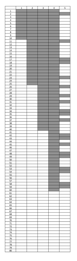
(a) Simulation Truth	(b) $\widehat{\bm{Z}}$ (under $\lambda^{2}=10,8$)	(c) $\widehat{\bm{Z}}$ ($\lambda^{2}=6$)

Figure 3: A simulation example. The plots show the feature allocation matrix $\bm{Z}$, with shaded area indicating $z_{sc}=1$, i.e., variant genotype. Rows are the SNVs and columns are the inferred haplotypes. Panel (a) shows the simulation truth ${\bm{Z}}^{o}$. Panel (b) displays the estimated feature allocation matrix $\widehat{\bm{Z}}$ for $\lambda^{2}=8$ and $10$. The estimate perfectly recovers the simulation truth. Panel (c) shows $\widehat{\bm{Z}}$ for $\lambda^{2}=6$. The first four haplotypes match the simulation truth.

We generated a data matrix with $S=80$ SNVs and $T=25$ samples. The simulation truth included $C^{o}=4$ latent haplotypes, plus a background haplotype that included all SNVs. The latent binary matrix ${\bm{Z}}^{o}$ was generated as follows: haplotype 1 was characterized by the presence of the first 10 SNVs, haplotype 2 by the first 25, haplotype 3 by the first 40 and haplotype 4 by the first 60. In other words, SNVs 1-10 occurred in all four haplotypes, SNVs 10-25 in haplotypes 2-4, SNVs 25-40 in haplotypes 3-4, SNVs 41-60 in haplotype 4 only, and SNVs 61-80 in none of the haplotypes. Figure 3(a) shows the simulation truth $\bm{Z}^{o}$. Let $\pi=(1,5,6,10)$ and $\pi_{p}$ be a random permutation of $\pi$, we generated true $\bm{w}_{t}^{o}\sim\mathrm{Dirichlet}(0.2,\pi_{p})$, $t=1,\dots,T$. Let $p^{o}_{0}=0.01$ and $N_{st}=50$ for all $s$ and $t$; we generated $n_{st}\sim\mathrm{Bin}(N_{st},p_{st})$, where $p_{st}=p_{0}^{o}w^{o}_{t0}+\sum_{c=1}^{C^{o}}w_{tc}^{o}z_{sc}^{o}$. We then ran the FL-means algorithm repeatedly with 1,000 random initializations to obtain a set of local minima of $Q$ as an approximate representation of posterior uncertainty. Each run of the FL-means algorithm only took 1 minute.

For different $\lambda^{2}$ values, we report point estimates (Figure 3 (b) and (c)) for $\bm{Z}$ that were obtained by minimizing the objective function $Q$. The point estimate is the estimate $(\widehat{C},\widehat{\bm{Z}},\widehat{w})$ that minimizes $Q(\bm{p})$ in 1,000 random initializations. Figure 4 shows the frequencies of the estimated number $\widehat{C}$ of features under different $\lambda^{2}$ values (the modes are highlighted by extra large plotting symbols). The plot shows the distribution of local minima over repeated runs of the algorithm with different initializations, all with the same simulated data.

Figure 4: The frequencies of estimated $\widehat{C}$ in 1000 simulations with different initializations. The mode is highlighted with extra large plotting symbols.

An important consideration in the implementation of the FL-means algorithm is the choice of the penalty parameter $\lambda^{2}$. As a sensitivity analysis we ran the FL-means algorithm with different $\lambda^{2}$ values: $\lambda^{2}=2,4,6,8,10,20,200$ and 500. Figure S1 (see Supplementary Material G) shows the estimated number $\widehat{C}$ of features and the realized minimum value of the objective function $Q$ versus $\lambda^{2}$. We observe that the $\widehat{C}$ decreases and the objective value increases as $\lambda^{2}$ increases. Summarizing Figures 3 and S1, we find that under $\lambda^{2}=8,10$, both the estimated $\widehat{C}$ and the estimated $\widehat{\bm{Z}}$ perfectly reconstruct the simulation truth $\bm{Z}^{o}$. Under $\lambda^{2}=6$, we find $\widehat{C}=5$ and the estimated $\widehat{\bm{Z}}$ includes true haplotypes (columns 1-4) as well as an additional spurious haplotype that includes some of the SNVs. We add a report of posterior uncertainties $\bar{p}_{sc}$, as defined in (14). In this particular case we find $\bar{p}_{sc}=1$ for all $s,c$. The estimate $\widehat{\bm{Z}}$ recovers the simulation truth, and there is little posterior uncertainty about it. As expected, a smaller $\lambda^{2}$ leads to a larger $\widehat{C}$ value. In summary, the inference summaries are sensitive with respect to the choice of $\lambda^{2}$. A good choice is critical. Below we suggest one reasonable ad-hoc algorithm for the choice of $\lambda^{2}$.

For comparisons, we applied a recently published method PyClone (Roth et al., , 2014) to the same simulated data. PyClone identifies candidate subclones as individual clusters by partitioning the SNVs into sets of similar VAFs. However, PyClone does not allow overlapping sets, that is, SNVs can not be shared across subclones, and is thus not fully in line with clonal evolution theory. Inference is still meaningful as a characterization of heterogeneity, but should be interpreted with care. To implement PyClone, we assumed that the copy number at SNVs was known. PyClone identified four clusters: cluster 1 consists of SNVs 1-25, cluster 2 SNVs 26-40, cluster 3 SNVs 41-60, and cluster 4 SNVs 61-80. The estimated cluster 1 includes the SNVs that appear in all the true haplotypes under the simulation truth; cluster 2 includes the SNVs from true haplotypes 3 and 4; cluster 3 includes the SNVs from true haplotypes 4 and cluster 4 includes the SNVs from none of the true haplotypes. Figure S2 plots the estimated mean cellular prevalence of each cluster across all the 25 samples. To summarize, in our simulation study PyClone did not recover the true haplotypes, which can not possibly be captured with non-overlapping clustering.

4.2 Subclone-Based Simulation

We carried out one more simulation study to evaluate the proposed FL-algorithm under model (7) for subclonal inference. We generated a data matrix with $S=80$ SNVs and $T=25$ samples. The simulation truth included $C^{o}=4$ latent subclones, plus a background subclone that included all SNVs. We generated the latent trinary matrix $\widetilde{{\bm{Z}}}^{o}$ as follows. We first generated a binary matrix ${\bm{Z}}^{o}$ as before, in Section 4.1. Next, if $z^{o}_{sc}=1$ then set $\widetilde{z}^{o}_{sc}=j$ with probabilities 0.7 (for $j=1$) and 0.3 (for $j=2$). If $z^{o}_{sc}=0$ then $\widetilde{z}^{o}_{sc}=0$. Figure S3(a) (Supplementary Material G) shows the simulation truth $\widetilde{\bm{Z}}^{o}$.

Next we fixed $p^{o}_{0}=0.01$ and $N_{st}=50$ and generated a simulation truth $\bm{w}_{t}^{o}$ as before, in Section 4.1. Finally, we generated $n_{st}\sim\mbox{Bin}(N_{st},p_{st})$, where $p_{st}=p_{0}^{o}w^{o}_{t0}+\frac{1}{2}\sum_{c=1}^{C^{o}}w_{tc}^{o}\widetilde{z}_{sc}^{o}$. We then ran the FL-means algorithm repeatedly with 1,000 random initializations to obtain a set of local minima of $Q$. The set of local minima provides the desired summary of the posterior distribution on the decomposition into subclones. We fix $\lambda^{2}$ using the algorithm from Section 4.3. As a result we estimated $\widehat{C}=4$, that is, we estimated the presence of four subclones. Figure S3(b) shows the estimated $\widetilde{\bm{Z}}$ under $\lambda^{2}=50$. In fact, posterior inference in this case perfectly recovered the simulation truth.

4.3 Calibration of $\lambda^{2}$

Recall that $w_{tc}$ denotes the relative fraction of haplotype $c$ in sample $t$. Under $\lambda^{2}=8$, the posterior estimate perfectly recovered the simulation truth. The estimates for $w_{tc}$ ranged from 0.01 to 0.53 for $c=1$, from 0.007 to 0.57 for $c=2$, from $1.8\times 10^{-8}$ to 0.52 for $c=3$ and from 0.008 to 0.59 for $c=4$ for $t=1,\dots,T$. Posterior inference (correctly) reports that each true haplotype $c$ constitutes a substantial part of the composition for some subset of samples. Under $\lambda^{2}=6$, the first four estimated features perfectly recover the simulation truth. However, for $c=5$, the estimated $w_{tc}$ ranged from $1.1\times 10^{-9}$ to 0.06. These very small fractions are biologically meaningless. We find similar patterns under $\lambda^{2}=2$ and 4. Based on these observations, we propose a heuristic to fix the tuning parameter $\lambda^{2}$. We start with a large value of $\lambda^{2}$, say, $\lambda^{2}=50$. While every imputed haplotype $c$ constitutes a substantial fraction in some subset of samples, say $w_{tc}>1/\widehat{C}$ for some $t$, we decrease $\lambda^{2}$ until newly imputed haplotypes only take small fraction in all samples, say, $w_{tc}<1/\widehat{C}$. The constant specified here is not arbitrary, instead, it can be chosen based on the biological questions that the researchers aim to address. For example, the haplotype prevalence below certain threshold is likely to be noise.

5 Results

5.1 Intra-Tumor Heterogeneity

We use deep DNA-sequencing data from an in-house experiment to study intra-TH that is characterizing heterogeneity of multiple samples in a single tumor. Data include four surgically dissected tumor samples from the same lung cancer patient. We performed whole-exome sequencing and processed the data using a bioinformatics pipeline consisting of standard procedures, such as base calling, read alignment, and variant calling. SNVs with VAFs close to 0 or 1 do not contribute to the heterogeneity analysis since these VAF values are expected when samples are homogeneous. We therefore remove these SNVs from the analysis. Details are given in the Supplementary Material H. The final number of SNVs for the four intra-tumor samples is $17,160$. With such a large data size, in practice it is infeasible to run the MCMC sampler proposed in Lee et al., (2013). PyClone is not designed to handle large-scale data sets. It took more than three days without returning any result, which makes it practically infeasible for high-throughput data analysis.

We first report inference based on haplotypes. Figure 5 summarizes the results. We fix $\lambda^{2}$ using the algorithm from Section 4.3, and find $\widehat{C}=3$ haplotypes. In Figure 5(a), we observe that haplotypes 1 and 2 have exactly complementary genotypes. Next we compare haplotypes 1 and 3. The second heatmap (still in panel a) plots only the 1,464 SNVs that differ between $c=1$ and $c=3$, highlighting the differences that are difficult to see in the earlier plot over all 17,160 SNVs. Three reported haplotypes imply that there are at least two subclones of tumor cells, one potentially with heterozygous mutations on the 17,160 SNVs, and another with an additional 1,464 somatic mutations. We annotated the 1,464 mutations and found that a large proportion of the mutations occur in known lung cancer biomarker genes. Some of them are de novo findings that will be further investigated.

Next we summarize posterior uncertainty by plotting $\bar{p}_{sc}$, as proposed in (14). This is shown in Figure 5(b). Green (light grey, $\bar{p}_{sc}=1$) means no posterior uncertainty. The plot in panel (b) is arranged exactly as in panel (a), with rows corresponding to SNVs and columns corresponding to haplotypes. The left plot shows all SNVs for all three haplotypes. The right plot zooms in on the subset of 1,464 SNVs that differ across $c=1$ and $3$ only, similar to panel (a). There is little posterior uncertainty about the 1,464 SNVs that differentiate haplotype 1 and haplotype 3. Figure 5(c) shows the circos plot (Krzywinski et al., , 2009) including the estimated proportion $\hat{w}_{tc}$ with $\widehat{C}=3$ haplotypes in each sample. Interestingly, four tumor samples possess similar proportions, indicating lack of spatial heterogeneity across four samples. This is not surprising as the four samples are taken from tumor regions that are geographically close.

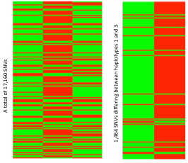
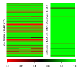
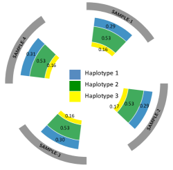
(a)	(b)	(c)

Figure 5: Summary of intra-TH analysis for four samples from a lung tumor with 17,160 SNVs. (a): The first heatmap shows posterior estimated haplotype genotypes (columns) of the selected SNVs. Three haplotypes are identified. A green/red block indicates a mutant/wildtype allele at the SNV in the haplotype. The second heatmap shows the differences between haplotypes 1 and 3 in the first heatmap. (b): The first heatmap shows the estimated uncertainties of three estimated haplotypes for 17,160 SNVs. The second heatmap shows the estimated uncertainties of 1,464 SNVs that differentiate haplotypes 1 and 3 in the first heatmap. (c): A circos plot showing the estimated proportion $\hat{w}_{tc}$ with $\widehat{C}=3$ haplotypes in each sample. The four samples possess similar proportions.

Next we consider a separate analysis using model (7) for inference on subclones. Posterior inference estimates $\widehat{C}=3$ subclones, and all four samples have similar proportions of the three subclones, with two subclones taking about 40% and 45% of the tumor content, and the third subclone taking about 15% of the tumor content in all four samples. This agrees with the reported haplotype proportions in Figure 5. However, the genotypes of subclones are expressed at 0, 1 or 2’s, representing homozygous reference, heterozygous and homozygous variant, respectively. Inference on subclones does not include inference on the constituent haplotypes, making it impossible to directly compare with the earlier analysis. However, we note that both analyses show that the four tumor samples are subclonal, and the subclone proportions are similar in all four samples. As a final model checking, Figure S4 shows the differences of $(p_{st}-\hat{p}_{st})$, where $\hat{p}_{st}$ is computed by plugging in the posterior estimates of $\bm{w}$ and $\bm{Z}$. As the figure shows, both analyses fit the data well.

5.2 Inter-Patients Tumor Heterogeneity

We analyzed exome-sequencing data for five tumor samples from patients with pancreatic ductal adenocarcinoma (PDAC) at NorthShore University HealthSystem (Lee et al., , 2013). Since samples were from different patients, we aimed to infer inter-patient TH. We applied models (4) and (7) for haplotype- and subclone-based inference, respectively. In both applications, we focused on a set of SNVs, and assumed that the collection of the genotypes at the SNVs could be shared between haplotypes in different tumor samples, regardless of the rest of the genome.

The mean sequencing depth for the samples was between 60X and 70X. A total of approximately 115,000 somatic SNVs were identified across the five whole exomes using GATK (McKenna et al., , 2010). First we focus on a small number of 118 SNVs selected with the following three criteria: (1) exhibit significant coverage in all samples; (2) occur within genes that are annotated to be related to PDAC in the KEGG pathways database (Kanehisa et al., , 2010); (3) are nonsynonymous, i.e., the mutation changes the amino acid sequence that is coded by the gene.

In summary, the PDAC data recorded the total read counts ($N_{st})$ and variant read counts ($n_{st}$) of $S=118$ SNVs from $T=5$ tumor samples. Figure S5 (see Supplementary Material G) shows the histogram of the observed VAFs, $n_{st}/N_{st}$. We ran the proposed FL-means algorithm with 1,000 random initializations. Each run of the FL-means algorithm took 50 seconds, while an MCMC sampler for finite feature allocation model proposed by Lee et al., (2013) took over one hour for each fixed number of haplotypes. Unlike MCMC, iterations of the FL-means algorithm are independent of each other. This facilitates parallel computing. For example, running all 1000 FL-means repetitions simultaneously the entire computation finished within one minute (instead of $>$10 hours if running sequentially). This is a significant speed advantage over MCMC simulation. After searching for reasonable values of $\lambda^{2}$ using the algorithm from Section 4.3, we estimated $\widehat{C}$ to be 5, i.e., five haplotypes.

Figure 6 summarizes the haplotype analysis results. In (a) we present an estimate of $\bm{Z}$, as the point estimate minimizing the objective function $Q$ in our runs. Each of the five columns represents a haplotype and each row represent an SNV, with green and red blocks indicating mutant and wildtype genotypes. In (b) we use a circos plot (Krzywinski et al., , 2009) to present the proportions of the five estimated haplotypes for each sample. Samples 1 and 5 possess the same three haplotypes (2, 4, and 5) while samples 2-4 all possess haplotype 1 and another distinct haplotype. The results show that most tumor samples consist of only two haplotypes, except samples 1 & 5, which have three haplotypes. No two samples share a complete set of haplotypes, reflecting the polymorphism between individuals. Lastly, haplotypes 1 , 4, and 5 are more prevalent than the other haplotypes, both appearing in three out of five samples. Haplotype 3 is the least prevalent appearing only in one sample. The corresponding uncertainties, as summarized by $\bar{p}_{sc}$, are shown in Figure S6 (a) (see Supplementary Material G).

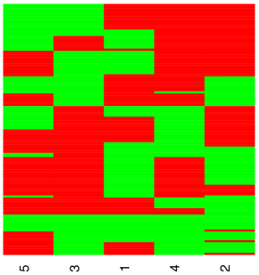
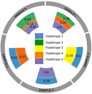
(a)	(b)

Figure 6: Summary of TH analysis using the PDAC data with 118 SNVs. (a): Posterior estimated haplotype genotypes (columns) of the selected SNVs. Five haplotypes are identified. A green/red block indicates a mutant/wildtype allele at the SNV in the haplotype. (b): A circos plot showing the estimated proportion $\hat{w}_{tc}$ with $\widehat{C}=5$ haplotypes.

For comparisons, we also applied PyClone to infer TH for the same pancreatic cancer data. PyClone identified 27 SNV clusters out of 118 samples, practically rendering the results hard to interpret and biologically less meaningful.

To examine the computational limits of the proposed approach we re-analyzed the PDAC data, but now keeping all SNVs that exhibit significant coverage in all samples and occur in at least two samples – not limited to those in KEGG pathways. This filtering left us with $S=6,599$ SNVs.

We applied the proposed FL-means algorithm with 1,000 random initializations. Each run of the FL-means algorithm took less than 2 minutes. After searching for $\lambda^{2}$ using the suggested heuristic, we estimated $\widehat{C}=7$. The full inference results are summarized in Figure 7. Interestingly, we found patterns that were similar to the previous analysis, such as that each sample possesses mostly two haplotypes. However, with more SNVs, there are now three (as opposed to one) distinct haplotypes, each only appearing in one out of five samples. This is not surprising since with more somatic SNVs, by definition the chance of having common haplotypes between different tumor samples will reduce. The heatmap in Figure S6 (b) (see Supplementary Material G) shows the estimated uncertainties of the estimated seven haplotypes.

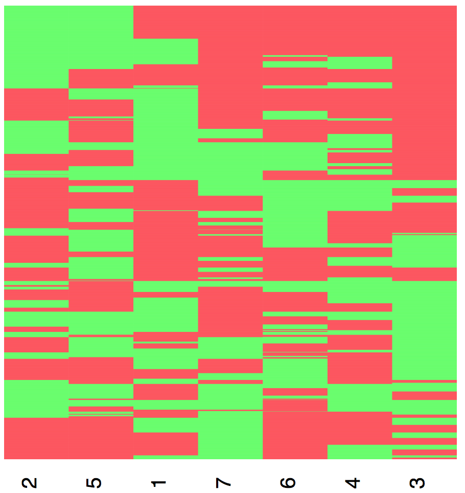
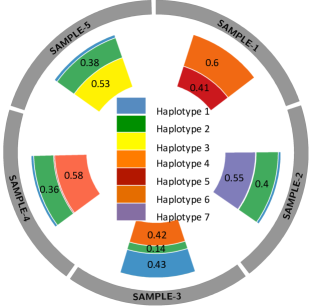
(a)	(b)

Figure 7: Summary of TH analysis using the PDAC data with 6,599 SNVs. (a): Posterior estimated haplotype genotypes (columns) of the selected SNVs. Seven haplotypes are identified. A green/red block indicates a mutant/wildtype allele at the SNV in the haplotype. (b): A circos plot showing the estimated proportion $\hat{w}_{tc}$ with $\widehat{C}=7$ haplotypes.

Lastly, we applied model (7) for subclonal inference across samples. Examining Figures 6(b) and 7(b), we see that most samples (except sample 1 in Figure 6(b)) possess two major haplotypes, which can be explained by having a single clone, i.e., no subclones. We observed the same results in subclonal inference: the five samples are clonal, each possessing a different local genome on the selected SNVs. While the results are less interesting, they suggest that the proposed models do not falsely infer subclonal structure where there is none.

6 Conclusion

We introduce small-variance asymptotics for the MAP in a feature allocation model under a binomial likelihood as it arises in inference for tumor heterogeneity. The proposed FL-algorithm uses a scaled version of the binomial likelihood that can be introduced as a special case of scaled exponential family models that are based on writing the sampling models in terms of Bregman divergences. The algorithm provides simple and scalable inference to feature allocation problems.

Inference in the three datasets shows that the proposed inference approaches correctly report subclonal or clonal inference for intra-TH and inter-patient TH. More importantly, haplotype inference reveals shared genotypes on selected SNVs recurring across samples. Such sharing would provide valuable information for future disease prognosis, taking advantage of the innovation proposed in this paper. For example, Ding et al., (2012) demonstrated that the relapse of acute myeloid leukemia was associated with new mutations acquired by a subpopulation of cancer cells derived from the original population.

In this paper we assumed diploidy or two copies of DNA for all genes. However, the copy number may vary in cancer cells, known as copy number variants (CNVs). SNVs and CNVs coexist throughout the genome. CNVs can alter the total read count mapped to a locus and eventually the observed VAFs. Integrating inference on both, CNVs and SNVs, to infer tumor heterogeneity could be a useful extension of the proposed model. Finally, in the proposed approach we implicitly treat normal tissue like any another subclone. If matching normal samples were available the model could be extended to borrow strength across tumor and normal samples by identifying a subpopulation of normal cells as part of the deconvolution.

Supplementary Material

Supplementary material is available under the Paper Information link at the JASA website.

References

- Andor et al., (2014) Andor, N., Harness, J. V., Müller, S., Mewes, H. W., and Petritsch, C. (2014). Expands: expanding ploidy and allele frequency on nested subpopulations. Bioinformatics, 30(1):50–60.
- Banerjee et al., (2005) Banerjee, A., Merugu, S., Dhillon, I. S., and Ghosh, J. (2005). Clustering with bregman divergences. The Journal of Machine Learning Research, 6:1705–1749.
- Bregman, (1967) Bregman, L. M. (1967). The relaxation method of finding the common point of convex sets and its application to the solution of problems in convex programming. USSR computational mathematics and mathematical physics, 7(3):200–217.
- (4) Broderick, T., Jordan, M. I., and Pitman, J. (2012a). Beta processes, stick-breaking and power laws. Bayesian analysis, 7(2):439–476.
- (5) Broderick, T., Kulis, B., and Jordan, M. I. (2012b). Mad-bayes: Map-based asymptotic derivations from bayes. arXiv preprint arXiv:1212.2126.
- Dempster et al., (1977) Dempster, A. P., Laird, N. M., and Rubin, D. B. (1977). Maximum likelihood from incomplete data via the em algorithm. Journal of the Royal Statistical Society. Series B (Methodological), pages 1–38.
- Ding et al., (2012) Ding, L., Ley, T. J., Larson, D. E., Miller, C. A., Koboldt, D. C., Welch, J. S., Ritchey, J. K., Young, M. A., Lamprecht, T., McLellan, M. D., et al. (2012). Clonal evolution in relapsed acute myeloid leukaemia revealed by whole-genome sequencing. Nature, 481(7382):506–510.
- Gerlinger et al., (2012) Gerlinger, M., Rowan, A. J., Horswell, S., Larkin, J., Endesfelder, D., Gronroos, E., Martinez, P., Matthews, N., Stewart, A., Tarpey, P., et al. (2012). Intratumor heterogeneity and branched evolution revealed by multiregion sequencing. New England Journal of Medicine, 366(10):883–892.
- Ghoshal, (2010) Ghoshal, S. (2010). The Dirichlet process, related priors and posterior asymptotics. In Nils Lid Hjort, Chris Holmes, P. M. and Walker, S. G., editors, Bayesian Nonparametrics, pages 22–34. Cambridge University Press.
- Green, (1995) Green, P. J. (1995). Reversible jump markov chain monte carlo computation and bayesian model determination. Biometrika, 82(4):711–732.
- Griffiths and Ghahramani, (2006) Griffiths, T. L. and Ghahramani, Z. (2006). Infinite latent feature models and the Indian buffet process. In Weiss, Y., Schölkopf, B., and Platt, J., editors, Advances in Neural Information Processing Systems 18, pages 475–482. MIT Press, Cambridge, MA.
- Hartigan and Wong, (1979) Hartigan, J. A. and Wong, M. A. (1979). Algorithm as 136: A k-means clustering algorithm. Journal of the Royal Statistical Society. Series C (Applied Statistics), 28(1):100–108.
- Hastie et al., (2001) Hastie, T., Tibshirani, R., and Friedman, J. J. H. (2001). The elements of statistical learning, volume 1. Springer New York.
- Kanehisa et al., (2010) Kanehisa, M., Goto, S., Furumichi, M., Tanabe, M., and Hirakawa, M. (2010). Kegg for representation and analysis of molecular networks involving diseases and drugs. Nucleic acids research, 38(suppl 1):D355–D360.
- Karlof, (2005) Karlof, J. K. (2005). Integer programming: theory and practice. CRC Press.
- Krzywinski et al., (2009) Krzywinski, M., Schein, J., Birol, I., Connors, J., Gascoyne, R., Horsman, D., Jones, S., and Marra, M. (2009). Circos: an information aesthetic for comparative genomics. Genome Res., 19(9):1639–45.
- Kulis and Jordan, (2011) Kulis, B. and Jordan, M. I. (2011). Revisiting k-means: New algorithms via bayesian nonparametrics. arXiv preprint arXiv:1111.0352.
- Landau et al., (2013) Landau, D. A., Carter, S. L., Stojanov, P., McKenna, A., Stevenson, K., Lawrence, M. S., Sougnez, C., Stewart, C., Sivachenko, A., Wang, L., et al. (2013). Evolution and impact of subclonal mutations in chronic lymphocytic leukemia. Cell, 152(4):714–726.
- Larson and Fridley, (2013) Larson, N. B. and Fridley, B. L. (2013). Purbayes: estimating tumor cellularity and subclonality in next-generation sequencing data. Bioinformatics, 29(15):1888–1889.
- Lee et al., (2013) Lee, J., Müller, P., Ji, Y., and Gulukota, K. (2013). A feature allocation model for tumor heterogeneity. Technical Report.
- Liu, (2008) Liu, J. S. (2008). Monte Carlo strategies in scientific computing. springer.
- McKenna et al., (2010) McKenna, A., Hanna, M., Banks, E., Sivachenko, A., Cibulskis, K., Kernytsky, A., Garimella, K., Altshuler, D., Gabriel, S., Daly, M., and Mark, D. (2010). The genome analysis toolkit: a MapReduce framework for analyzing next-generation DNA sequencing data. Genome research, 20(9):1297–1303.
- Roth et al., (2014) Roth, A., Khattra, J., Yap, D., Wan, A., Laks, E., Biele, J., Ha, G., Aparicio, S., Bouchard-Côté, A., and Shah, S. P. (2014). Pyclone: statistical inference of clonal population structure in cancer. Nature methods.
- Teh et al., (2007) Teh, Y. W., Görür, D., and Ghahramani, Z. (2007). Stick-breaking construction for the indian buffet process. In International Conference on Artificial Intelligence and Statistics, pages 556–563.
- Thibaux and Jordan, (2007) Thibaux, R. and Jordan, M. (2007). Hierarchical beta processes and the indian buffet process. In Proceedings of the 11th Conference on Artificial Intelligence and Statistics (AISTAT), Puerto Rico.