Łojasiewicz inequalities and applications

Abstract.

In real algebraic geometry, Lojasiewicz’s theorem asserts that any integral curve of the gradient flow of an analytic function that has an accumulation point has a unique limit. Lojasiewicz proved this result in the early 1960s as a consequence of his gradient inequality.

Many problems in calculus of variations are questions about critical points or gradient flow lines of an infinite dimensional functional. Perhaps surprisingly, even blowups at singularities of many nonlinear PDE’s can, in a certain sense, be thought of as limits of infinite dimensional gradient flows of analytic functionals. Thus, the question of uniqueness of blowups can be approached as an infinite dimensional version of Lojasiewicz’s theorem. The question of uniqueness of blowups is perhaps the most fundamental question about singularities.

This approach to uniqueness was pioneered by Leon Simon thirty years ago for the area functional and many related functionals using an elaborate reduction to a finite dimensional setting where Lojasiewicz’s arguments applied.

Recently, the authors proved two new infinite dimensional Lojasiewicz inequalities at noncompact singularities where it was well-known that a reduction to Lojasiewicz’s arguments is not possible, but instead entirely new techniques are required. As a consequence, the authors settled a major long-standing open question about uniqueness of blowups for mean curvature flow (MCF) at all generic singularities and for mean convex MCF at all singularities. Using this, the authors have obtained a rather complete description of the space-time singular set for MCF with generic singularities. In particular, the singular set of a MCF in ${\mathbb{R}}^{n+1}$ with only generic singularities is contained in finitely many compact Lipschitz submanifolds of dimension at most $n-1$ together with a set of dimension at most $n-2$.

0. Finite and infinite dimensional inequalities

0.1. Lojasiewicz inequalities

In real algebraic geometry, the Lojasiewicz inequality, [L1], [L2], [L4], from the late 1950s named after Stanislaw Lojasiewicz, gives an upper bound for the distance from a point to the nearest zero of a given real analytic function. Specifically, let $f:U\to{\mathbb{R}}$ be a real-analytic function on an open set $U$ in ${\mathbb{R}}^{n}$, and let $Z$ be the zero locus of $f$. Assume that $Z$ is not empty. Then for any compact set $K$ in $U$, there exist $\alpha\geq 2$ and a positive constant $C$ such that, for all $x\in K$

(0.1) $$\inf_{z\in Z}|x-z|^{\alpha}\leq C\,|f(x)|\,.$$

Here $\alpha$ can be large.

Equation (0.1) was the main inequality in Lojasiewicz’s proof of Laurent Schwarz’s division conjecture in analysis. Around the same time, Hörmander, [Hö], independently proved Schwarz’s division conjecture in the special case of polynomials and a key step in his proof was also (0.1) when $f$ is a polynomial.

A few years later, Lojasiewicz solved a conjecture of Whitney in [L3] using the following inequality: With the same assumptions on $f$, for every $p\in U$, there are a possibly smaller neighborhood $W$ of $p$ and constants $\beta\in(0,1)$ and $C>0$ such that for all $x\in W$

(0.2) $$|f(x)-f(p)|^{\beta}\leq C\,|\nabla_{x}f|\,.$$

Note that this inequality is trivial unless $p$ is a critical point for $f$.

One immediate consequence of (0.2) is that every critical point of $f$ has a neighborhood where every other critical point has the same value. It is easy to construct smooth functions where this is not the case.

0.2. First Lojasiewicz implies the second

In this subsection, we will explain how the second Lojasiewicz inequality for a function $f$ in a neighborhood of an isolated critical point follows from the first. To make things concrete, we will show that the second holds with $\beta=\frac{2}{3}$ when the first holds with $\alpha=2$.

Suppose that $f:{\mathbb{R}}^{n}\to{\mathbb{R}}$ is smooth function with $f(0)=0$ and $\nabla f(0)=0$; without loss of generality, we may assume that the Hessian is in diagonal form at $0$ and we will write the coordinates as $x=(y,z)$ where $y$ are the coordinates where the Hessian is nondegenerate. By Taylor’s formula in a small neighborhood of $0$, we have that

(0.3) $$f(x) =\frac{a_{i}}{2}\,y_{i}^{2}+O(|x|^{3})\,.$$

(0.4) $$f_{y_{i}}(x) =a_{i}\,y_{i}+O(|x|^{2})\,.$$

(0.5) $$f_{z_{i}}(x) =O(|x|^{2})\,.$$

It follows from this that the second of the two Lojasiewicz inequalities holds for $f$ and $\beta=\frac{2}{3}$ provided that $|z|^{2}\leq\epsilon\,|y|$ for some sufficiently small $\epsilon>0$. Namely, if $|z|^{2}\leq\epsilon\,|y|$, then

(0.6) $$C\,|y|\leq|\nabla_{x}f|{\text{ and }}|f(x)|\leq C^{-1}\,|y|^{\frac{3}{2}}$$

for some positive constant $C$ and, hence,

(0.7) $$|f(x)|^{\frac{2}{3}}\leq C\,|\nabla_{x}f|\,.$$

Therefore, we only need to prove the second Lojasiewicz inequality for $f$ in the region $|z|^{2}\geq\epsilon\,|y|$. We will do this using the first Lojasiewicz inequality for $\nabla f$. Since $0$ is an isolated critical point for $f$, the first Lojasiewicz inequality for $\nabla f$ gives that

(0.8) $$|\nabla_{x}f|\geq C\,|x|^{2}\,.$$

By assumption on the region and the Taylor expansion for $f$, we get that in this region

(0.9) $$|f(x)|\leq C\,|y|^{2}+C\,|z|^{3}\leq C\,|z|^{3}\leq C\,|x|^{3}\,.$$

Combining these two inequalities gives

(0.10) $$|f(x)|^{\frac{2}{3}}\leq C\,|x|^{2}\leq|\nabla_{x}f|\,.$$

This proves the second Lojasiewicz inequality for $f$ with $\beta=\frac{2}{3}$.

Lojasiewicz used his second inequality to show the “Lojasiewicz theorem”: If $f:{\mathbb{R}}^{n}\to{\mathbb{R}}$ is an analytic function, $x=x(t):[0,\infty)\to{\mathbb{R}}^{n}$ is a curve with $x^{\prime}(t)=-\nabla f$ and $x(t)$ has a limit point $x_{\infty}$, then the length of the curve is finite and

(0.11) $$\lim_{t\to\infty}x(t)=x_{\infty}\,.$$

Moreover, $x_{\infty}$ is a critical point for $f$.

In contrast, it is easy to construct smooth functions, even on ${\mathbb{R}}^{2}$, where the Lojasiewicz theorem fails, i.e., where there are negative gradient flow lines that have more than one limit point (and, thus, also have infinite length); see Figure 1.

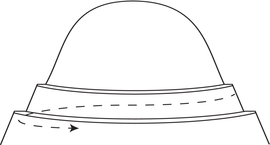
Figure 1. There are smooth functions vanishing on an open (compact) set for which the gradient flow lines spiral around the zero locus. The flow lines have infinite length and the Lojasiewicz theorem fails.

0.3. The Lojasiewicz Theorem

Next we will explain how the second Lojasiewicz inequality is typically used to show uniqueness. Before we do that, observe first that in the second inequality we always work in a small neighborhood of $p$ so that, in particular, $|f(x)-f(p)|\leq 1$ and hence smaller powers on the left hand side of the inequality imply the inequality for higher powers. As it turns out, we will see that any positive power strictly less than one would do for uniqueness.

Suppose that $f:{\mathbb{R}}^{n}\to{\mathbb{R}}$ is a differentiable function. Let $x=x(t)$ be a curve in ${\mathbb{R}}^{n}$ parametrized on $[0,\infty)$ whose velocity $x^{\prime}=-\nabla f$. We would like to show that if the second inequality of Lojasiewicz holds for $f$ with a power $1>\beta>1/2$, then the Lojasiewicz theorem mentioned above holds. That is, if $x(t)$ has a limit point $x_{\infty}$, then the length of the curve is finite and $\lim_{t\to\infty}x(t)=x_{\infty}$. Since $x_{\infty}$ is a limit point of $x(t)$ and $f$ is non-increasing along the curve, $x_{\infty}$ must be a critical point for $f$.

The length of the curve $x(t)$ is $\int|\nabla f|$, so we must show that $\int_{1}^{\infty}|\nabla f|\,ds$ is finite. Assume that $f(x_{\infty})=0$ and note that if we set $f(t)=f(x(t))$, then $f^{\prime}=-|\nabla f|^{2}$. Moreover, by the second Lojasiewicz inequality, we get that $f^{\prime}\leq-f^{2\beta}$ if $x(t)$ is sufficiently close to $x_{\infty}$. (Assume for simplicity below that $x(t)$ stays in a small neighborhood $x_{\infty}$ for $t$ sufficiently large so that this inequality holds; the general case follows with trivial changes.) Then this inequality can be rewritten as $(f^{1-2\beta})^{\prime}\geq(2\beta-1)$ which integrates to

(0.12) $$f(t)\leq C\,t^{\frac{-1}{2\beta-1}}\,.$$

We need to show that (0.12) implies that $\int_{1}^{\infty}|\nabla f|\,ds$ is finite. This shows that $x(t)$ converges to $x_{\infty}$ as $t\to\infty$. To see that $\int_{1}^{\infty}|\nabla f|\,ds$ is finite, observe by the Cauchy-Schwarz inequality that

(0.13) $$\int_{1}^{\infty}|\nabla f|\,ds=\int_{1}^{\infty}\sqrt{-f^{\prime}}\,ds\leq\left(-\int_{1}^{\infty}f^{\prime}\,s^{1+\epsilon}\,ds\right)^{\frac{1}{2}}\left(\int_{1}^{\infty}s^{-1-\epsilon}\,ds\right)^{\frac{1}{2}}\,.$$

It suffices therefore to show that

(0.14) $$-\int_{1}^{T}f^{\prime}\,s^{1+\epsilon}\,ds$$

is uniformly bounded. Integrating by parts gives

(0.15) $$\int_{1}^{T}f^{\prime}\,s^{1+\epsilon}\,ds=|f\,s^{1+\epsilon}|^{T}_{1}-(1+\epsilon)\int_{1}^{T}f\,s^{\epsilon}\,ds\,.$$

If we choose $\epsilon>0$ sufficiently small depending on $\beta$, then we see that this is bounded independent of $T$ and hence $\int_{1}^{\infty}|\nabla f|\,ds$ is finite.

0.4. Infinite dimensional Lojasiewicz inequalities and applications

Many problems in geometry and the calculus of variations are essentially questions about functionals on infinite dimensional spaces, such as the energy functional on the space of mappings or the area functional on the space of graphs over a hypersurface. Infinite dimensional versions of Lojasiewicz inequalities, proven in a celebrated work of Leon Simon, [Si1], have played an important role in these areas over the last 30 years. Clearly, the infinite dimensional inequalities have immediate applications to uniqueness of limits for gradient flows, but, perhaps surprisingly, they also have implications for singularities of nonlinear PDE’s.

Once singularities occur one naturally wonders what the singularities are like. A standard technique for analysing singularities is to magnify around them. Unfortunately, singularities in many of the interesting problems in Geometric-PDE looked at under a microscope will resemble one blowup, but under higher magnification, it might (as far as anyone knows) resemble a completely different blowup. Whether this ever happens is perhaps the most fundamental question about singularities; see, e.g., [Si2] and [Hr]. By general principles, the set of blowups is connected and, thus, the difficulty for uniqueness is when the blowups are not isolated in the space of blowups.

One of the first major results on uniqueness was by Allard-Almgren in 1981, [AA], where uniqueness of tangent cones with smooth cross-section for minimal varieties is proven under an additional integrability assumption on the cross-section. The integrability condition applies in a number of important cases, but it is difficult to check and is not satisfied in many other important cases.

Perhaps surprisingly, blowups for a number of important Geometric PDE’s can essentially be reformulated as infinite dimensional gradient flows of analytic functionals. Thus, the uniqueness question would follow from an infinite dimensional version of Lojasiewicz’s theorem for gradient flows of analytic functionals. Infinite dimensional versions of Lojasiewicz inequalities were proven in a celebrated work of Leon Simon, [Si1], for the area, energy, and related functionals and used, in particular, to prove a fundamental result about uniqueness of tangent cones with smooth cross-section of minimal surfaces. This holds, for instance, at all singular points of an area-minimizing hypersurface in ${\mathbb{R}}^{8}$.

Lojasiewicz inequalities follow easily near a critical point where the Hessian is uniformly non-degenerate (this is the infinite dimensional analog of a non-degenerate critical point where the Hessian is full rank). The difficulty is dealing with the directions in the kernel of the Hessian. In the cases that Simon considers, the Hessian has finite dimensional kernel by elliptic theory. The rough idea of his approach is to use the easy argument in the (infinitely many) directions where the Hessian is invertible and use the classical Lojasiewicz inequalities on the finite dimensional kernel. He makes this rigorous by reducing the infinite dimensional version to the classical Lojasiewicz inequality using Lyapunov-Schmidt reduction. Infinite dimensional Lojasiewicz inequalities proven using Lyapunov-Schmidt reduction, as in the work of Simon, have had a profound impact on various areas of analysis and geometry and are usually referred to as Lojasiewicz-Simon inequalities.

The cross-sections of the tangent cones at the singularities in these cases are assumed to be smooth and compact and this is crucial. This means that nearby cross-sections can be written as graphs over the cross-section and, thus, can be identified with functions on the cross-section of the cone. The problem is then to prove a Lojasiewicz-Simon inequality for an analytic functional on a Banach space of functions, where $0$ is a critical point corresponding to the cross-section.

Uniqueness of tangents has important applications to regularity of the singular set; see Section 5 and cf., e.g., [Si3], [Si4], [Si5], [BrCoL] and [HrLi] and cf. Figure 2.

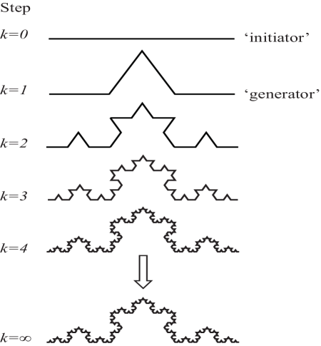
Figure 2. The Koch curve is close to a line on all scales, yet the line that it is close to changes from scale to scale. It is not rectifiable but admits a Hölder parametrization. It also illustrates that uniqueness of blowups is closely related to rectifiability.

1. Uniqueness of blowups for mean curvature flow

In the next few sections, we will explain why at each generic singularity of a mean curvature flow the blowup is unique; that is independent of the sequence of rescalings; see Figure 3. This very recent result settled a major open problem that was open even in the case of mean convex hypersurfaces where it was known that all singularities are generic. Moreover, it is the first general uniqueness theorem for blowups to a Geometric-PDE at a non-compact singularity.

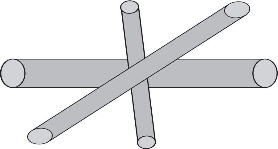
Figure 3. The essence of uniqueness of tangent flows: Can the flow be close to a cylinder at all times right before the singular time, yet the axis of the cylinder changes as the time gets closer to the singular time?

As already mentioned uniqueness of blowups is perhaps the most fundamental question that one can ask about singularities and is known to imply regularity of the singular set.

The proof of this uniqueness result relies on two completely new infinite dimensional Lojasiewicz type inequalities that, unlike all other infinite dimensional Lojasiewicz inequalities we know of, do not follow from reduction to the classical finite-dimensional Lojasiewicz inequalities, but rather are proven directly and do not rely on Lojasiewicz’s arguments or results.

It is well-known that to deal with non-compact singularities requires entirely new ideas and techniques as one cannot argue as in Simon’s work, and all the later work that uses his ideas. Partly because of this, it is expected that the techniques and ideas described here have applications to other flows.

The rest of this paper focuses on mean curvature flow (or MCF) of hypersurfaces. This is a non-linear parabolic evolution equation where a hypersurface evolves over time by locally moving in the direction of steepest descent for the volume element. It has been used and studied in material science for almost a century. Unlike some of the other earlier papers in material science, both von Neumann’s 1952 paper and Mullins 1956 paper had explicit equations. In his paper von Neumann discussed soap foams whose interface tend to have constant mean curvature whereas Mullins is describing coarsening in metals, in which interfaces are not generally of constant mean curvature. Partly as a consequence, Mullins may have been the first to write down the MCF equation in general. Mullins also found some of the basic self-similar solutions like the translating solution now known as the Grim Reaper. To be precise, suppose that $M_{t}\subset{\mathbb{R}}^{n+1}$ is a one-parameter family of smooth hypersurfaces, then we say that $M_{t}$ flows by the MCF if

(1.1) $$x_{t}=-H\,{\bf{n}}\,,$$

where $H$ and ${\bf{n}}$ are the mean curvature and unit normal, respectively, of $M_{t}$ at the point $x$.

1.1. Tangent flows

By definition, a tangent flow is the limit of a sequence of rescalings at a singularity, where the convergence is uniform on compact subsets. For instance, a tangent flow to $M_{t}$ at the origin in space-time is the limit of a sequence of rescaled flows $\frac{1}{\delta_{i}}\,M_{\delta_{i}^{2}\,t}$ where $\delta_{i}\to 0$. A priori, different sequences $\delta_{i}$ could give different tangent flows and the question of the uniqueness of the blowup - independent of the sequence - is a major question in many geometric problems. By a monotonicity formula of Huisken, [H1], and an argument of Ilmanen and White, [I], [W3], tangent flows are shrinkers, i.e., self-similar solutions of MCF that evolve by rescaling. The only generic shrinkers are round cylinders by [CM1].

We will say that a singular point is cylindrical if at least one tangent flow is a multiplicity one cylinder $\SS^{k}\times{\mathbb{R}}^{n-k}$. The main application of the new Lojasiewicz type inequality of [CM2] is the following theorem that shows that tangent flows at generic singularities are unique:

Theorem .

[CM2] Let $M_{t}$ be a MCF in ${\mathbb{R}}^{n+1}$. At each cylindrical singular point the tangent flow is unique. That is, any other tangent flow is also a cylinder with the same ${\mathbb{R}}^{k}$ factor that points in the same direction.

This theorem solves a major open problem; see, e.g., page $534$ of [W2]. Even in the case of the evolution of mean convex hypersurfaces where all singularities are cylindrical, uniqueness of the axis was unknown; see [HS1], [HS2], [W1], [W4], [SS], [An] and [HaK].

In recent joint work with Tom Ilmanen, [CIM], we showed that if one tangent flow at a singular point of a MCF is a multiplicity one cylinder, then all are. However, [CIM] left open the possibility that the direction of the axis (the ${\mathbb{R}}^{k}$ factor) depended on the sequence of rescalings. The proof of Theorem 1.1 and, in particular, the first Lojasiewicz type inequality of [CM2], has its roots in some ideas and inequalities from [CIM] and in fact implicitly use that cylinders are isolated among shrinkers by [CIM].

The results of [CM2] are the first general uniqueness theorems for tangent flows to a geometric flow at a non-compact singularity. (In fact, not only are the singularities that [CM2] deal with non-compact but they are also non-integrable.) Some special cases of uniqueness of tangent flows for MCF were previously analyzed assuming either some sort of convexity or that the hypersurface is a surface of rotation; see [H1], [H2], [HS1], [HS2], [W1], [SS], [AAG], section $3.2$ in the book [GGS], and [GK], [GKS], [GS]. In contrast, uniqueness for blowups at compact singularities is better understood; cf. [AA], [Si1], [H3], [Sc], [KSy], and [Se].

One of the significant difficulties that [CM2] overcomes, and sets it apart from all other work we know of, is that the singularities are noncompact. This causes major analytical difficulties and to address them requires entirely new techniques and ideas. This is not so much because of the subtleties of analysis on noncompact domains, though this is an issue, but crucially because the evolving hypersurface cannot be written as an entire graph over the singularity no matter how close we get to the singularity. Rather, the geometry of the situation dictates that only part of the evolving hypersurface can be written as a graph over a compact piece of the singularity.

2. Lojasiewicz inequalities for non-compact hypersurfaces and MCF

The infinite dimensional Lojasiewicz-type inequalities that [CM2] showed are for the $F$-functional on the space of hypersurfaces.

The $F$-functional is given by integrating the Gaussian over a hypersurface $\Sigma\subset{\mathbb{R}}^{n+1}$. This is also often referred to as the Gaussian surface area and is defined by

(2.1) $$F(\Sigma)=(4\pi)^{-n/2}\,\int_{\Sigma}\,{\text{e}}^{-\frac{|x|^{2}}{4}}\,d\mu\,.$$

The entropy $\lambda(\Sigma)$ is the supremum of the Gaussian surface areas over all centers and scales

(2.2) $$\lambda(\Sigma)=\sup_{t_{0}>0,\,x_{0}\in{\mathbb{R}}^{n}}\,\,(4\pi\,t_{0})^{-n/2}\,\int_{\Sigma}\,{\text{e}}^{-\frac{|x-x_{0}|^{2}}{4t_{0}}}\,d\mu\,.$$

The entropy is a Lyapunov functional for both MCF and rescaled MCF (it is monotone non-increasing under the flows).

It follows from the first variation formula that the gradient of $F$ is

(2.3) $$\nabla_{\Sigma}F(\psi)=\int_{\Sigma}\,\left(H-\frac{\langle x,{\bf{n}}\rangle}{2}\right)\,\psi\,{\text{e}}^{-\frac{|x|^{2}}{4}}\,.$$

Thus, the critical points of $F$ are shrinkers, i.e., hypersurfaces with $H=\frac{\langle x,{\bf{n}}\rangle}{2}$. The most important shrinkers are the generalized cylinders ${\mathcal{C}}$; these are the generic ones by [CM1]. The space ${\mathcal{C}}$ is the union of ${\mathcal{C}}_{k}$ for $k\geq 1$, where ${\mathcal{C}}_{k}$ is the space of cylinders $\SS^{k}\times{\mathbb{R}}^{n-k}$, where the $\SS^{k}$ is centered at $0$ and has radius $\sqrt{2k}$ and we allow all possible rotations by $SO(n+1)$.

A family of hypersurfaces $\Sigma_{s}$ evolves by the negative gradient flow for the $F$-functional if it satisfies the equation

(2.4) $$(\partial_{s}x)^{\perp}=-H\,{\bf{n}}+x^{\perp}/2\,.$$

This flow is called the rescaled MCF since $\Sigma_{s}$ is obtained from a MCF $M_{t}$ by setting $\Sigma_{s}=\frac{1}{\sqrt{-t}}M_{t}$, $s=-\log(-t)$, $t<0$. By (2.3), critical points for the $F$-functional or, equivalently, stationary points for the rescaled MCF, are the shrinkers for the MCF that become extinct at the origin in space-time. A rescaled MCF has a unique asymptotic limit if and only if the corresponding MCF has a unique tangent flow at that singularity.

The paper [CM2] proved versions of the two Lojasiewicz inequalities for the $F$-functional on a general hypersurface $\Sigma$. Roughly speaking, [CM2] showed that

(2.5) $${\text{dist}}(\Sigma,{\mathcal{C}})^{2} \leq C\,\left|\nabla_{\Sigma}F\right|\,,$$

(2.6) $$(F(\Sigma)-F({\mathcal{C}}))^{\frac{2}{3}} \leq C\,\left|\nabla_{\Sigma}F\right|\,.$$

Equation (2.5) corresponds to Lojasiewicz’s first inequality for $\nabla F$ whereas (2.6) corresponds to his second inequality for $F$. The precise statements of these inequalities are much more complicated than this, but they are of the same flavor.

As noted earlier a consequence of the classical Lojasiewicz gradient inequality for an analytical function on Euclidean space is that near a critical point there is no other critical values. This consequence of a Lojasiewicz gradient inequality for the $F$-functional near a round cylinder (and in fact the corresponding consequence of (2.5)) was established in earlier joint work with Tom Ilmanen (see [CIM] for the precise statement):

Theorem .

[CIM] Any shrinker that is sufficiently close to a round cylinder on a large, but compact, set must itself be a round cylinder.

In [CM2] an infinite dimensional analog of the first Lojasiewicz inequality is proven directly and used together with an infinite dimensional analog of the argument in Subsection 0.2 to show an analog of the second Lojasiewicz inequality. As mentioned, the reason why one cannot argue as in Simon’s work, and all the later work that makes use his ideas, comes from that the singularities are noncompact.

2.1. The two Lojasiewicz inequalities

We will now state the two Lojasiewicz-type inequalities for the $F$-functional on the space of hypersurfaces.

Suppose that $\Sigma\subset{\mathbb{R}}^{n+1}$ is a hypersurface and fix some sufficiently small $\epsilon_{0}>0$. Given a large integer $\ell$ and a large constant $C_{\ell}$, we let ${\bf{r}}_{\ell}(\Sigma)$ be the maximal radius so that

• $B_{{\bf{r}}_{\ell}(\Sigma)}\cap\Sigma$ is the graph over a cylinder in ${\mathcal{C}}_{k}$ of a function $u$ with $\|u\|_{C^{2,\alpha}}\leq\epsilon_{0}$ and $|\nabla^{\ell}A|\leq C_{\ell}$.

In the next theorem, we will use a Gaussian $L^{2}$ distance $d_{{\mathcal{C}}}(R)$ to the space ${\mathcal{C}}_{k}$ in the ball of radius $R$. To define this, given $\Sigma_{k}\in{\mathcal{C}}_{k}$, let $w_{\Sigma_{k}}:{\mathbb{R}}^{n+1}\to{\mathbb{R}}$ denote the distance to the axis of $\Sigma_{k}$ (i.e., to the space of translations that leave $\Sigma_{k}$ invariant). Then we define

(2.7) $$d_{{\mathcal{C}}}^{2}(R)=\inf_{\Sigma_{k}\in{\mathcal{C}}_{k}}\,\|w_{\Sigma_{k}}-\sqrt{2k}\|_{L^{2}(B_{R})}^{2}\equiv\inf_{\Sigma_{k}\in{\mathcal{C}}_{k}}\,\int_{B_{R}\cap\Sigma_{k}}(w_{\Sigma_{k}}-\sqrt{2k})^{2}\,{\text{e}}^{-\frac{|x|^{2}}{4}}\,.$$

The Gaussian $L^{p}$ norm on the ball $B_{R}$ is $\|u\|^{p}_{L^{p}(B_{R})}=\int_{B_{R}}|u|^{p}\,{\text{e}}^{-\frac{|x|^{2}}{4}}$.

Given a general hypersurface $\Sigma$, it is also convenient to define the function $\phi$ by

(2.8) $$\phi=\frac{\langle x,{\bf{n}}\rangle}{2}-H\,,$$

so that $\phi$ is minus the gradient of the functional $F$.

The main tools that [CM2] developed are the following two analogs for non-compact hypersurfaces of Lojasiewicz’s inequalities. The first of these inequalities is really for the gradient whereas the second is for the function.

Theorem .

(A Lojasiewicz inequality for non-compact hypersurfaces, [CM2]). If $\Sigma\subset{\mathbb{R}}^{n+1}$ is a hypersurface with $\lambda(\Sigma)\leq\lambda_{0}$ and $R\in[1,{\bf{r}}_{\ell}(\Sigma)-1]$, then

(2.9) $$d^{2}_{{\mathcal{C}}}(R)\leq C\,R^{\rho}\,\left\{\|\phi\|_{L^{1}(B_{R})}^{b_{\ell,n}}+{\text{e}}^{-\frac{b_{\ell,n}\,R^{2}}{4}}\right\}\,,$$

where $C=C(n,\ell,C_{\ell},\lambda_{0})$, $\rho=\rho(n)$ and $b_{\ell,n}\in(0,1)$ satisfies $\lim_{\ell\to\infty}\,b_{\ell,n}=1$.

The theorem bounds the $L^{2}$ distance to ${\mathcal{C}}_{k}$ by a power of $\|\phi\|_{L^{1}}$, with an error term that comes from a cutoff argument since $\Sigma$ is non-compact and is not globally a graph of the cylinder. This theorem is essentially sharp. Namely, the estimate (2.9) does not hold for any exponent $b_{\ell,n}$ larger than one, but Theorem 2.1 lets us take $b_{\ell,n}$ arbitrarily close to one.

In [CM2] it is shown that the above inequality implies the following gradient type Lojasiewicz inequality. This inequality bounds the difference of the $F$ functional near a critical point by two terms. The first is essentially a power of $\nabla F$, while the second (exponentially decaying) term comes from that $\Sigma$ is not a graph over the entire cylinder.

Theorem .

(A gradient Lojasiewicz inequality for non-compact hypersurfaces, [CM2]). If $\Sigma\subset{\mathbb{R}}^{n+1}$ is a hypersurface with $\lambda(\Sigma)\leq\lambda_{0}$, $\beta\in[0,1)$, and $R\in[1,{\bf{r}}_{\ell}(\Sigma)-1]$, then

(2.10) $$\left|F(\Sigma)-F({\mathcal{C}}_{k})\right| \leq C\,R^{\rho}\,\left\{\|\phi\|_{L^{2}(B_{R})}^{c_{\ell,n}\,\frac{3+\beta}{2+2\beta}}+{\text{e}}^{-\frac{c_{\ell,n}\,(3+\beta)R^{2}}{8(1+\beta)}}+{\text{e}}^{-\frac{(3+\beta)(R-1)^{2}}{16}}\,\right\}\,,$$

where $C=C(n,\ell,C_{\ell},\lambda_{0})$, $\rho=\rho(n)$ and $c_{\ell,n}\in(0,1)$ satisfies $\lim_{\ell\to\infty}\,c_{\ell,n}=1$.

When the theorem is applied, the parameters $\beta$ and $\ell$ is chosen to make the exponent greater than one on the $\nabla F$ term, essentially giving that $\left|F(\Sigma)-F({\mathcal{C}}_{k})\right|$ is bounded by a power greater than one of $|\nabla F|$. A separate argument is needed to handle the exponentially decaying error terms.

The paper [CM2] showed that when $\Sigma_{t}$ are flowing by the rescaled MCF, then both terms on the right-hand side of (2.10) are bounded by a power greater than one of $\|\phi\|_{L^{2}}$ (the corresponding statement holds for Theorem 2.1). Thus, one essentially get the inequalities

(2.11) $$d_{{\mathcal{C}}}^{2} \leq C\,\left|\nabla_{\Sigma_{t}}F\right|\,,$$

(2.12) $$(F(\Sigma_{t})-F({\mathcal{C}}))^{\frac{2}{3}} \leq C\,\left|\nabla_{\Sigma_{t}}F\right|\,.$$

These two inequalities can be thought of as analogs for the rescaled MCF of Lojasiewicz inequalities; cf. (2.5) and (2.6).

3. Cylindrical estimates for a general hypersurface

The proof of the two Lojasiewicz inequalities relies on some equations and estimates on general hypersurfaces $\Sigma\subset{\mathbb{R}}^{n+1}$. Particularly important are bounds for $\nabla\frac{A}{H}$ when the mean curvature $H$ is positive on a large set. This will be discussed in this section.

3.1. A general Simons equation

An important point for the proof of the Lojasiewicz type inequalities is that the second fundamental form $A$ of $\Sigma$ satisfies an elliptic differential equation similar to Simons’ equation for minimal surfaces. The elliptic operator will be the $L$ operator from [CM1] given by

(3.1) $$L\equiv{\mathcal{L}}+|A|^{2}+\frac{1}{2}\equiv\Delta-\frac{1}{2}\,\nabla_{x^{T}}+|A|^{2}+\frac{1}{2}\,,$$

where we have the following:

Proposition .

[CM2] If $\phi=\frac{1}{2}\langle x,{\bf{n}}\rangle-H$, then

(3.2) $$L\,A=A+{\text{Hess}}_{\phi}+\phi\,A^{2}\,,$$

where the tensor $A^{2}$ is given in orthonormal frame by $\left(A^{2}\right)_{ij}=A_{ik}\,A_{kj}$.

Note that $\phi$ vanishes precisely when $\Sigma$ is a shrinker and, in this case, we recover the Simons’ equation for $A$ for shrinkers from [CM1].

3.2. An integral bound when the mean curvature is positive

One of the keys in the proof of the first Lojasiewicz type inequality is that the tensor $\tau=A/H$ is almost parallel when $H$ is positive and $\phi$ is small. This generalizes an estimate from [CIM] in the case where $\Sigma$ is a shrinker (i.e., $\phi\equiv 0$) with $H>0$.

Given $f>0$, define a weighted divergence operator ${\text{div}}_{f}$ and drift Laplacian ${\mathcal{L}}_{f}$ by

(3.3) $${\text{div}}_{f}(V) =\frac{1}{f}\,{\text{e}}^{|x|^{2}/4}\,{\text{div}}_{\Sigma}\,\left(f\,{\text{e}}^{-|x|^{2}/4}\,V\right)\,,$$

(3.4) $${\mathcal{L}}_{f}\,u \equiv{\text{div}}_{f}(\nabla u)={\mathcal{L}}\,u+\langle\nabla\log f,\nabla u\rangle\,.$$

Here $u$ may also be a tensor; in this case the divergence traces only with $\nabla$. Note that ${\mathcal{L}}={\mathcal{L}}_{1}$. We recall the quotient rule (see lemma $4.3$ in [CIM]):

Lemma .

Given a tensor $\tau$ and a function $g$ with $g\neq 0$, then

(3.5) $${\mathcal{L}}_{g^{2}}\,\frac{\tau}{g} =\frac{g\,{\mathcal{L}}\,\tau-\tau\,{\mathcal{L}}\,g}{g^{2}}=\frac{g\,L\,\tau-\tau\,L\,g}{g^{2}}\,.$$

Proposition .

[CM2] On the set where $H>0$, we have

(3.6) $${\mathcal{L}}_{H^{2}}\,\frac{A}{H} =\frac{{\text{Hess}}_{\phi}+\phi\,A^{2}}{H}+\frac{A\,\left(\Delta\phi+\phi\,|A|^{2}\right)}{H^{2}}\,,$$

(3.7) $${\mathcal{L}}_{H^{2}}\,\frac{|A|^{2}}{H^{2}} =2\,\left|\nabla\frac{A}{H}\right|^{2}+2\,\frac{\langle{\text{Hess}}_{\phi}+\phi\,A^{2},A\rangle}{H^{2}}+2\,\frac{|A|^{2}\,\left(\Delta\phi+\phi\,|A|^{2}\right)}{H^{3}}\,.$$

The proposition follows easily from Proposition 3.1 and the Leibniz rule of Lemma 3.2; see [CM2] for details.

The next proposition gives exponentially decaying integral bounds for $\nabla(A/H)$ when $H$ is positive on a large ball. It will be important that these bounds decay rapidly.

Proposition .

[CM2] If $B_{R}\cap\Sigma$ is smooth with $H>0$, then for $s\in(0,R)$ we have

$$\int_{B_{R-s}\cap\Sigma}\left|\nabla\frac{A}{H}\right|^{2}\,H^{2}\,{\text{e}}^{-\frac{|x|^{2}}{4}} \leq\frac{4}{s^{2}}\,\sup_{B_{R}\cap\Sigma}|A|^{2}\,{\text{Vol}}(B_{R}\cap\Sigma)\,{\text{e}}^{-\frac{(R-s)^{2}}{4}}$$

(3.8) $$\quad+2\,\int_{B_{R}\cap\Sigma}\left\{\left|\langle{\text{Hess}}_{\phi},A\rangle+\frac{|A|^{2}}{H}\,\Delta\phi\right|+\left|\langle A^{2},A\rangle+\frac{|A|^{4}}{H}\right|\,|\phi|\right\}{\text{e}}^{-\frac{|x|^{2}}{4}}\,.$$

Proof.

Set $\tau=A/H$ and $u=|\tau|^{2}=|A|^{2}/H^{2}$. It will be convenient within this proof to use square brackets $\left[\cdot\right]$ to denote Gaussian integrals over $B_{R}\cap\Sigma$, i.e. $\left[f\right]=\int_{B_{R}\cap\Sigma}f\,{\text{e}}^{-|x|^{2}/4}$.

Let $\psi$ be a function with support in $B_{R}$. Using the divergence theorem, the formula from Proposition 3.2 for ${\mathcal{L}}_{H^{2}}u$, and the absorbing inequality $4ab\leq a^{2}+4b^{2}$, we get

$$0 =\left[{\text{div}}_{H^{2}}\,\left(\psi^{2}\,\nabla u\right)\,H^{2}\left]=\right[\left(\psi^{2}\,{\mathcal{L}}_{H^{2}}u+2\psi\langle\nabla\psi,\nabla u\rangle\right)\,H^{2}\right]$$

$$=\left[\left\{2\,\psi^{2}\,\left|\nabla\tau\right|^{2}+2\,\psi^{2}\left(\frac{\langle{\text{Hess}}_{\phi}+\phi\,A^{2},A\rangle}{H^{2}}+\frac{|A|^{2}\,\left(\Delta\phi+\phi\,|A|^{2}\right)}{H^{3}}\right)+4\psi\langle\nabla\psi,\tau\cdot\nabla\tau\rangle\right\}\,H^{2}\right]$$

$$\geq\left[\left(\psi^{2}\,\left|\nabla\tau\right|^{2}-4\,|\tau|^{2}\,\left|\nabla\psi\right|^{2}\right)\,H^{2}\,\right]+2\,\left[\psi^{2}\langle{\text{Hess}}_{\phi}+\phi\,A^{2},A\rangle\right]+2\,\left[\psi^{2}\frac{|A|^{2}\,\left(\Delta\phi+\phi\,|A|^{2}\right)}{H}\right]\,,$$

from which we obtain

$$\left[\psi^{2}\,\left|\nabla\tau\right|^{2}\,H^{2}\right] \leq 4\,\left[\left|\nabla\psi\right|^{2}\,|A|^{2}\,\right]-2\,\left[\psi^{2}\,\langle{\text{Hess}}_{\phi}+\phi A^{2},A\rangle\right]-2\,\left[\psi^{2}\,\Delta\phi\,\frac{|A|^{2}}{H}+\psi^{2}\,\phi\frac{|A|^{4}}{H}\right]\,.$$

The proposition follows by choosing $\psi\equiv 1$ on $B_{R-s}$ and going to zero linearly on $\partial B_{R}$. ∎

This proposition has the the following corollary:

Corollary .

[CM2] If $B_{R}\cap\Sigma$ is smooth with $H>\delta>0$ and $|A|\leq C_{1}$, then there exists $C_{2}=C_{2}(n,\delta,C_{1})$ so that for $s\in(0,R)$ we have

(3.9) $$\int_{B_{R-s}\cap\Sigma}\left|\nabla\frac{A}{H}\right|^{2}\,{\text{e}}^{-\frac{|x|^{2}}{4}} \leq\frac{C_{2}}{s^{2}}\,{\text{Vol}}(B_{R}\cap\Sigma)\,{\text{e}}^{-\frac{(R-s)^{2}}{4}}+C_{2}\,\int_{B_{R}\cap\Sigma}\left\{\left|{\text{Hess}}_{\phi}\right|+|\phi|\right\}{\text{e}}^{-\frac{|x|^{2}}{4}}\,.$$

Remark .

Corollary 3.2 essentially bounds the distance squared to the space of cylinders by $\|\phi\|_{L^{1}}$. This is sharp: it is not possible to get the sharper bound where the powers are the same. This is a general fact when there is a non-integrable kernel. Namely, if we perturb in the direction of the kernel, then $\phi$ vanishes quadratically in the distance.

The next corollary combines the Gaussian $L^{2}$ bound on $\nabla\tau$ from Corollary 3.2 with standard interpolation inequalities to get pointwise bounds on $\nabla\tau$ and $\nabla^{2}\tau$.

Corollary .

[CM2] If $B_{R}\cap\Sigma$ is smooth with $H>\delta>0$, $|A|+\left|\nabla^{\ell+1}A\right|\leq C_{1}$, and $\lambda(\Sigma)\leq\lambda_{0}$, then there exists $C_{3}=C_{3}(n,\lambda_{0},\delta,\ell,C_{1})$ so that for $|y|+\frac{1}{1+|y|}<R-1$, we have

(3.10) $$\left|\nabla\,\frac{A}{H}\right|(y)+\left|\nabla^{2}\frac{A}{H}\right|(y) \leq C_{3}\,R^{2n}\,\left\{{\text{e}}^{-d_{\ell,n}\,\frac{(R-1)^{2}}{8}}+\|\phi\|_{L^{1}(B_{R})}^{\frac{d_{\ell,n}}{2}}\right\}\,{\text{e}}^{\frac{|y|^{2}}{8}}\,,$$

where the exponent $d_{\ell,n}\in(0,1)$ has $\lim_{\ell\to\infty}d_{\ell,n}=1$.

See [CM2] for the proof of Corollary 3.2.

4. Distance to cylinders and the first Lojasiewicz inequality

Finally, we will briefly outline how one get from Corollary 3.2 to the proof of the first Lojasiewicz type inequality for the $F$-functional. This inequality will follow from the bounds on the tensor $\tau=\frac{A}{H}$ in the previous section together with the following proposition:

Proposition .

[CM2] Given $n$, $\delta>0$ and $C_{1}$, there exist $\epsilon_{0}>0$, $\epsilon_{1}>0$ and $C$ so that if $\Sigma\subset{\mathbb{R}}^{n+1}$ is a hypersurface (possibly with boundary) that satisfies:

1. $H\geq\delta>0$ and $|A|+|\nabla A|\leq C_{1}$ on $B_{R}\cap\Sigma$.

2. $B_{5\sqrt{2n}}\cap\Sigma$ is $\epsilon_{0}$ $C^{2}$-close to a cylinder in ${\mathcal{C}}_{k}$ for some $k\geq 1$,

then, for any $r\in(5\sqrt{2n},R)$ with

(4.1) $$r^{2}\,\sup_{B_{5\sqrt{2n}}}\left(|\phi|+|\nabla\phi|\right)+r^{5}\,\sup_{B_{r}}\left(|\nabla\tau|+|\nabla^{2}\tau|\right)\leq\epsilon_{1}\,,$$

we have that $B_{\sqrt{r^{2}-3k}}\cap\Sigma$ is the graph over (a subset of) a cylinder in ${\mathcal{C}}_{k}$ of $u$ with

(4.2) $$|u|+|\nabla u|\leq C\,\left\{r^{2}\,\sup_{B_{5\sqrt{2n}}}\left(|\phi|+|\nabla\phi|\right)+r^{5}\,\sup_{B_{r}}\left(|\nabla\tau|+|\nabla^{2}\tau|\right)\right\}\,.$$

This proposition shows that $\Sigma$ must be close to a cylinder as long as $H$ is positive, $\phi$ is small, $\tau$ is almost parallel and $\Sigma$ is close to a cylinder on a fixed small ball. Together with Tom Ilmanen, we proved a similar result in proposition $2.2$ in [CIM] in the special case where $\Sigma$ is a shrinker (i.e., when $\phi\equiv 0$) and this proposition is inspired by that one.

To prove Proposition 4 we make use of the following result from [CIM] (see corollary $4.22$ in [CIM]):

Lemma .

[CIM] If $\Sigma\subset{\mathbb{R}}^{n+1}$ is a hypersurface (possibly with boundary) with

• $0<\delta\leq H$ on $\Sigma$,

• the tensor $\tau\equiv A/H$ satisfies $\left|\nabla\tau\right|+\left|\nabla^{2}\tau\right|\leq\epsilon\leq 1$,

• At the point $p\in\Sigma$, $\tau_{p}$ has at least two distinct eigenvalues $\kappa_{1}\neq\kappa_{2}$,

then

$$\left|\kappa_{1}\kappa_{2}\right|\leq\frac{2\,\epsilon}{\delta^{2}}\,\left(\frac{1}{\left|\kappa_{1}-\kappa_{2}\right|}+\frac{1}{\left|\kappa_{1}-\kappa_{2}\right|^{2}}\right)\,.$$

From this lemma, we see that if the assumption of the lemma holds for a hypersurface, then the principal curvatures divide into two groups. One group consists of principal curvatures that are close to zero and the other group consists of principal curvatures that cluster around a non-zero real number. Thus, we get flatness for any two-plane containing a principal direction in the first group, while any two-plane spanned by principal directions in the second group is umbilic. This is the starting point for the proof of Proposition 4.

5. The singular set of MCF with generic singularities

A major theme in PDE’s over the last fifty years has been understanding singularities and the set where singularities occur. In the presence of a scale-invariant monotone quantity, blowup arguments can often be used to bound the dimension of the singular set; see, e.g., [Al], [F]. Unfortunately, these dimension bounds say little about the structure of the set. However, using the results of the previous sections, [CM3] gave a rather complete description of the singular set for MCF with generic singularities.

The main result of [CM3] is the following:

Theorem ([CM3]).

Let $M_{t}\subset{\mathbb{R}}^{n+1}$ be a MCF of closed embedded hypersurfaces with only cylindrical singularities, then the space-time singular set satisfies:

• It is contained in finitely many (compact) embedded Lipschitz submanifolds each of dimension at most $(n-1)$ together with a set of dimension at most $(n-2)$.

• It consists of countably many graphs of $2$-Hölder functions on space.

• The time image of each subset with finite parabolic $2$-dimensional Hausdorff measure has measure zero; each such connected subset is contained in a time-slice.

In fact, [CM3] proves considerably more than what is stated in Theorem 5; see theorem $4.18$ in [CM3]. For instance, instead of just proving the first claim of the theorem, the entire stratification of the space-time singular set is Lipschitz of the appropriate dimension. Moreover, this holds without ever discarding any subset of measure zero of any dimension as is always implicit in any definition of rectifiable. To illustrate the much stronger version, consider the case of evolution of surfaces in ${\mathbb{R}}^{3}$. In that case, this gives that the space-time singular set is contained in finitely many (compact) embedded Lipschitz curves with cylinder singularities together with a countable set of spherical singularities. In higher dimensions, the direct generalization of this is proven.

Theorem 5 has the following corollaries:

Corollary ([CM3]).

Let $M_{t}\subset{\mathbb{R}}^{n+1}$ be a MCF of closed embedded mean convex hypersurfaces or a MCF with only generic singularities, then the conclusion of Theorem 1.1 holds.

More can be said in dimensions three and four:

Corollary ([CM3]).

If $M_{t}$ is as in Theorem 5 and $n=2$ or $3$, then the evolving hypersurface is completely smooth (i.e., without any singularities) at almost all times. In particular, any connected subset of the space-time singular set is completely contained in a time-slice.

Corollary ([CM3]).

For a generic MCF in ${\mathbb{R}}^{3}$ or ${\mathbb{R}}^{4}$ or a flow starting at a closed embedded mean convex hypersurface in ${\mathbb{R}}^{3}$ or ${\mathbb{R}}^{4}$ the conclusion of Corollary 5 holds.

The conclusions of Corollary 5 hold in all dimensions if the initial hypersurface is $2$- or $3$-convex. A hypersurface is said to be $k$-convex if the sum of any $k$ principal curvatures is nonnegative.

A key technical point in [CM3] is to prove a strong parabolic Reifenberg property for MCF with generic singularities. In fact, the space-time singular set is proven to be (parabolically) Reifenberg vanishing. In Analysis a subset of Euclidean space is said to be Reifenberg (or Reifenberg flat) if on all sufficiently small scales it is, after rescaling to unit size close, to a $k$-dimensional plane. The dimension of the plane is always the same but the plane itself may change from scale to scale. Many snowflakes, like the Koch snowflake, are Reifenberg with Hausdorff dimension strictly larger than one. A set is said to be Reifenberg vanishing if the closeness to a $k$-plane goes to zero as the scale goes to zero. It is said to have the strong Reifenberg property if the $k$-dimensional plane depends only on the point but not on the scale. Finally, one sometimes distinguishes between half Reifenberg and full Reifenberg, where half Reifenberg refers to that the set is close to a $k$-dimensional plane, whereas full Reifenberg refers to that in addition one also has the symmetric property: The plane on the given scale is close to the set.

Using the results from [CM2] described earlier in this paper, [CM3] shows that the singular set in space-time is strong (half) Reifenberg vanishing with respect to the parabolic Hausdorff distance. This is done in two steps, showing first that nearby singularities sit inside a parabolic cone (i.e., between two oppositely oriented space-time paraboloids that are tangent to the time-slice through the singularity). In fact, this parabolic cone property holds with vanishing constant. Next, in the complementary region of the parabolic cone in space-time (that is essentially space-like), the parabolic Reifenberg essentially follows from the space Reifenberg that the uniqueness of [CM2] of tangent flows implies.

An immediate consequence, of independent interest, of our parabolic cone property with vanishing constant is that nearby a generic singularity in space-time (nearby is with respect to the parabolic distance) all other singularities happen at almost the same time.

These results should be contrasted with a result of Altschuler-Angenent-Giga, [AAG] (cf. [SS]), that shows that in ${\mathbb{R}}^{3}$ the evolution of any rotationally symmetric surface obtained by rotating the graph of a function $r=u(x)$, $a<x<b$ around the $x$-axis is smooth except at finitely many singular times where either a cylindrical or spherical singularity forms. For more general rotationally symmetric surfaces (even mean convex), the singularities can consist of nontrivial curves. For instance, consider a torus of revolution bounding a region $\Omega$. If the torus is thin enough, it will be mean convex. Since the symmetry is preserved and because the surface always remains in $\Omega$, it can only collapse to a circle. Thus at the time of collapse, the singular set is a simple closed curve. White showed that a mean convex surface evolving by MCF in ${\mathbb{R}}^{3}$ must be smooth at almost all times, and at no time can the singular set be more than $1$-dimensional (see section $5$ in [W2]). In all dimensions, White showed that the space-time singular set of a mean convex MCF has parabolic Hausdorff dimension at most $(n-1)$; see [W1] and cf. theorem $1.15$ in [HaK]. In fact, White’s general dimension reducing argument gives that the singular set of any MCF with only cylindrical singularities has dimension at most $(n-1)$.

These results motivate the following conjecture:

Conjecture ([CM3]).

Let $M_{t}$ be a MCF of closed embedded hypersurfaces in ${\mathbb{R}}^{n+1}$ with only cylindrical singularities. Then the space-time singular set has only finitely many components.

If this conjecture was true, then it would follow from this paper that in ${\mathbb{R}}^{3}$ and ${\mathbb{R}}^{4}$ mean curvature flow with only generic singularities is smooth except at finitely many times; cf. with the three-dimensional conjecture at the end of section $5$ in [W2].

References

- [AA] W.K. Allard and F.J. Almgren, Jr, On the radial behavior of minimal surfaces and the uniqueness of their tangent cones. Ann. of Math. (2) 113 (1981), no. 2, 215–265.
- [AAG] S. Altschuler, S.B. Angenent, and Y. Giga, Mean curvature flow through singularities for surfaces of rotation, Journal of geometric analysis, Volume 5, Number 3, (1995) 293–358.
- [Al] F. J. Almgren, Jr., Q-valued functions minimizing dirichlet’s integral and the regularity of area minimizing rectiable currents up to codimension two, preprint.
- [An] B. Andrews, Noncollapsing in mean-convex mean curvature flow. Geom. Topol. 16 (2012), no. 3, 1413–1418.
- [BrCoL] H. Brezis, J.-M. Coron and E. Lieb, Harmonic maps with defects, Comm. Math. Phys. 107 (1986), no. 4, 649–705.
- [CIM] T.H. Colding, T. Ilmanen and W.P. Minicozzi II, Rigidity of generic singularities of mean curvature flow, publications IHES, to appear, arXiv:1304.6356.
- [CM1] T.H. Colding and W.P. Minicozzi II, Generic mean curvature flow I; generic singularities, Annals of Math., Volume 175 (2012), Issue 2, 755–833.
- [CM2] by same author, Uniqueness of blowups and Łojasiewicz inequalities, Annals of Math, to appear, http://arXiv:1312.4046.
- [CM3] by same author, The singular set of mean curvature flow with generic singularities, preprint, arXiv:1405.5187.
- [F] H. Federer, The singular sets of area minimizing rectifiable currents with codimension one and of area minimizing flat chains modulo two with arbitrary codimension. Bull. Amer. Math. Soc. 76 (1970) 767–771.
- [FFl] H. Federer and W. Fleming, Normal and integral currents, Ann. of Math. 72 (1960), 458–520.
- [GK] Z. Gang and D. Knopf, Universality in mean curvature flow neckpinches, http://arxiv.org/abs/1308.5600.
- [GKS] Z. Gang, D. Knopf, and I.M. Sigal, Neckpinch dynamics for asymmetric surfaces evolving by mean curvature flow, preprint, http://arXiv:1109.0939v1.
- [GS] Z. Gang and I.M. Sigal, Neck pinching dynamics under mean curvature flow, preprint, http://arxiv.org/abs/0708.2938.
- [GGS] M. Giga, Y. Giga, and J. Saal, Nonlinear partial differential equations. Asymptotic behavior of solutions and self-similar solutions. Progress in Nonlinear Differential Equations and their Applications, 79. Birkhäuser Boston, Inc., Boston, MA, 2010.
- [Hr] R.M. Hardt, Singularities of harmonic maps. Bull. Amer. Math. Soc. (N.S.) 34 (1997), no. 1, 15–34.
- [HrLi] R.M. Hardt and F.-H. Lin, Stability of singularities of minimizing harmonic maps. J. Differential Geom. 29 (1989), no. 1, 113–123.
- [HaK] R. Haslhofer and B. Kleiner, Mean curvature flow of mean convex hypersurfaces, preprint, http://arXiv:1304.0926.
- [Hö] L. Hörmander, On the division of distributions by polynomials, Ark. Mat. 3 (1958) 555–568.
- [H1] G. Huisken, Asymptotic behavior for singularities of the mean curvature flow. J. Differential Geom. 31 (1990), no. 1, 285–299.
- [H2] by same author, Local and global behaviour of hypersurfaces moving by mean curvature. Differential geometry: partial differential equations on manifolds (Los Angeles, CA, 1990), 175–191, Proc. Sympos. Pure Math., 54, Part 1, Amer. Math. Soc., Providence, RI, 1993.
- [H3] by same author, Flow by mean curvature of convex surfaces into spheres, J. Differential Geometry 20 (1984) 237-266.
- [HS1] G. Huisken and C. Sinestrari, Convexity estimates for mean curvature flow and singularities of mean convex surfaces, Acta Math. 183 (1999) no. 1, 45–70.
- [HS2] G. Huisken and C. Sinestrari, Mean curvature flow singularities for mean convex surfaces, Calc. Var. Partial Differ. Equ. 8 (1999), 1–14.
-
[I]
T. Ilmanen,
Singularities of Mean Curvature Flow of Surfaces, preprint, 1995,
http://www.math.ethz.ch/~/papers/pub.html. - [KSy] R. Kohn and S. Serfaty, A deterministic-control-based approach to motion by curvature, Comm. Pure Appl. Math. 59 (2006), no. 3, 344–407.
- [L1] S. Łojasiewicz, Ensembles semi-analytiques, IHES notes (1965).
- [L2] by same author, Sur le probl me de la division, Studia Math. 18 (1959) 87–136.
- [L3] by same author, Une propriété topologique des sous-ensembles analytiques réels, Les Équations aux Dérivées Partielles (1963) pp. 87–89, CNRS, Paris.
- [L4] by same author, Division d’une distribution par une fonction analytique de variables rélles. C. R. Acad. Sci. Paris 246, 683–686 (1958) (Séance du 3 Février 1958).
- [Sc] F. Schulze, Uniqueness of compact tangent flows in mean curvature flow, J. Reine Angew. Math. 690 (2014), 163 172.
- [Se] N. Sesum, Rate of convergence of the mean curvature flow. Comm. Pure Appl. Math. 61 (2008), no. 4, 464–485.
- [Si1] L. Simon, Asymptotics for a class of evolution equations, with applications to geometric problems, Annals of Math. 118 (1983), 525–571.
- [Si2] by same author, A general asymptotic decay lemma for elliptic problems. Handbook of geometric analysis. No. 1, 381–411, Adv. Lect. Math. (ALM), 7, Int. Press, Somerville, MA, 2008.
- [Si3] by same author, Rectifiability of the singular set of energy minimizing maps, Calc. Var. Partial. Differential Equations 3 (1995), no. 1, 1–65.
- [Si4] by same author, Theorems on regularity and singularity of energy minimizing maps, Lectures on geometric variational problems (Sendai, 1993), 115–150, Springer, Tokyo, 1996.
- [Si5] by same author, Rectifiability of the singular sets of multiplicity 1 minimal surfaces and energy minimizing maps, Surveys in differential geometry, Vol. II (Cambridge, MA, 1993), 246–305, Int. Press, Cambridge, MA, 1995.
- [SS] H. Soner and P. Souganidis, Singularities and uniqueness of cylindrically symmetric surfaces moving by mean curvature. Comm. Partial Differential Equations 18 (1993), no. 5-6, 859–894.
- [T] J. Taylor, Regularity of the singular sets of two-dimensional area-minimizing flat chains modulo 3 in , Invent. Math. 22 (1973), 119–159.
- [W1] B. White, The nature of singularities in mean curvature flow of mean-convex sets. J. Amer. Math. Soc. 16 (2003), no. 1, 123–138.
- [W2] by same author, Evolution of curves and surfaces by mean curvature. Proceedings of the International Congress of Mathematicians, Vol. I (Beijing, 2002), 525–538.
- [W3] by same author, Partial regularity of mean-convex hypersurfaces flowing by mean curvature, Int. Math. Res. Notices (1994) 185–192.
- [W4] by same author, Subsequent singularities in mean-convex mean curvature flow, arXiv:1103.1469, 2011.