Self-sustaining turbulence in a restricted nonlinear model of plane Couette flow

Abstract

This paper demonstrates the maintenance of self-sustaining turbulence in a restricted nonlinear (RNL) model of plane Couette flow. The RNL system is derived directly from the Navier Stokes equations and permits computationally tractable studies of the dynamical system obtained using stochastic structural stability theory (S3T), which is a second order approximation of the statistical state dynamics of the flow. The RNL model shares the dynamical restrictions of the S3T model but can be easily implemented through reducing a DNS code to the equations governing the RNL system. Comparisons of turbulence arising from DNS and RNL simulations demonstrate that the RNL system supports self-sustaining turbulence with a mean flow as well as structural and dynamical features that are consistent with DNS. These results demonstrate that the simplified RNL/S3T system captures fundamental aspects of fully developed turbulence in wall-bounded shear flows and motivates use of the RNL/S3T system for further study of wall turbulence.

I Introduction

The Navier Stokes (NS) equations provide a comprehensive model for the dynamics of turbulence. Unfortunately, these equations are analytically intractable. They have, however, been extensively studied computationally since the pioneering work of Kim, Moin, and Moser (1987) and a number of highly resolved numerical simulations exist, see e.g. Simens et al. (2009); del Álamo et al. (2004); Tsukahara, Kawamura, and Shingai (2006); Hoyas and Jimenez (2008). Ever increasing computing power will continue progress toward simulating an increasingly wider range of turbulent flows. However, a complete understanding of the physical mechanisms underlying turbulence in the NS equations, even in simple parallel flow configurations, remains elusive. Thus, considerable effort has been devoted to the search for more tractable models that characterize the dynamics of turbulence.

The Linearized Navier Stokes (LNS) equations are a particularly appealing model because they can be analyzed using well developed tools from linear systems theory Farrell and Ioannou (1996a, b). They have been used extensively to characterize energy growth and disturbance amplification in wall bounded shear flows, in particular the large disturbance amplification that arises from the non-normal linear operators governing these flows Farrell (1988); Gustavsson (1991); Trefethen et al. (1993); Reddy and Henningson (1993); Farrell and Ioannou (1993a); Bamieh and Dahleh (2001); Jovanović and Bamieh (2005). The LNS equations capture the energy production of the full nonlinear system Henningson (1996) and linear non-normal growth mechanisms have been shown to be necessary for subcritical transition to turbulence Henningson and Reddy (1994). The LNS equations also provide insight into the mechanism maintaining turbulence. In particular, the linear coupling between the Orr-Sommerfeld and Squire equations is required to generate the wall layer streaks that are a necessary component of the process maintaining turbulence in wall-bounded shear flowsButler and Farrell (1993); Kim and Lim (2000). In this context, the term “streak” describes the “well-defined elongated region of spanwise alternating bands of low and high speed fluid” (Waleffe, Kim, and Hamilton, 1991). The LNS equations have also been used to predict second-order statistics Jovanović and Bamieh (2001); Jovanović and Georgiou (2010) and the spectra of turbulent channel flows Butler and Farrell (1993); Farrell and Ioannou (1998); del Álamo and Jiménez (2006); Hwang and Cossu (2010); Cossu, Pujals, and Depardon (2009); Moarref and Jovanović (2012). The above results and a host of others illustrate the power of the LNS equations as a model for studying physical mechanisms in wall-bounded turbulence. While the LNS equations provide insight into the mechanisms underlying turbulence, there are two fundamental aspects of turbulence that the LNS system is unable to model: the turbulent mean velocity profile and the mechanism that maintains turbulence.

Empirical models have also proven useful in capturing certain aspects of turbulent flows. For example, Proper Orthogonal Decomposition (POD) has been used to construct low dimensional ordinary differential equation models of turbulent flows, see e.g. Lumley (1967); Smith, Moehlis, and Holmes (2005). However, empirical models of this type are based on data resulting from experiments or simulations rather than proceeding directly from the NS equations. This limitation is shared by eddy viscosity models.

Researchers have also sought insight into turbulence through examining numerically obtained three-dimensional equilibria and periodic orbits of the NS equations, see e.g. Jiménez et al. (2005); Kawahara, Uhlmann, and Van Veen (2012). For plane Couette flow, the first such numerical solution was computed by Nagata (1990). Details concerning these numerically obtained fixed points and periodic orbits for plane Couette flow can be found in Gibson, Halcrow, and Cvitanović (2009); Kawahara, Uhlmann, and Van Veen (2012). These solutions reflect local properties of the attractor and the extension of these solutions to the global turbulent dynamics has yet to be completed.

The 2D/3C model Reynolds and Kassinos (1995); Bobba, Bamieh, and Doyle (2002); Gayme et al. (2010) is a recent attempt to obtain an analytically tractable simplified model derived from the NS equations. The assumptions underlying this model are based on experimental Kim and Adrian (1999); Guala, Hommema, and Adrian (2006); Hutchins and Marusic (2007) and analytical evidence Farrell and Ioannou (1993a); Jovanović and Bamieh (2005); Cossu, Pujals, and Depardon (2009); McKeon and Sharma (2010) of the central role of streamwise coherent structures in wall turbulence. This streamwise constant model has been used to accurately simulate the mean turbulent velocity profile Gayme et al. (2010), to identify the large-scale spanwise spacing of the streamwise coherent structures and to study the energetics of fully developed turbulent plane Couette flows Gayme et al. (2011). The primary limitation of the 2D/3C model is that it supports only one-way interactions from the perturbation field to the mean flow and as a consequence it requires persistent stochastic excitation to sustain the turbulent state perturbations. In fact, the laminar solution of the unforced 2D/3C model has been shown to be globally asymptotically stable Bobba (2004).

The current work describes a more comprehensive model that is similar to the 2D/3C model in its use of a streamwise constant mean flow, but which also incorporates two-way interaction between this streamwise constant mean flow and the perturbation field. This coupling is chosen to parallel that used in the Stochastic Structural Stability Theory (S3T) model Farrell and Ioannou (2003). The S3T equations comprise the joint evolution of the streamwise constant mean flow (first cumulant) and the ensemble second order perturbation statistics (second cumulant), and can be viewed as a second order closure of the dynamics of the statistical state. These equations are closed either by parameterizing the higher cumulants as a stochastic excitation Farrell and Ioannou (1993a); DelSole and Farrell (1996); DelSole (2004) or by setting the third cumulant to zero, see e.g Marston, Conover, and Schneider (2008); Tobias, Dagon, and Marston (2011); Srinivasan and Young (2012). This restriction of the NS equations to the first two cumulants involves parameterizing or neglecting the perturbation-perturbation interactions in the full nonlinear system and retaining only the interaction between the perturbations and the instantaneous mean flow. This closure results in a nonlinear autonomous dynamical system that governs evolution of the statistical state of the turbulence comprised of this mean flow and the second order perturbation statistics. A simulation of the restricted nonlinear (RNL) system may be regarded as a statistical state dynamics obtained from a single member of the ensemble making up the S3T dynamics.

The S3T model has recently been used to study the dynamics of fully developed wall turbulence Farrell et al. (2012), in particular that of the roll and streak structures. These prominent features of wall-turbulence were first identified in the buffer layer Kline et al. (1967). Rolls and streaks have often been suggested to play a central role in maintaining wall turbulence but neither the laminar nor the turbulent streamwise mean velocity profile give rise to these structures as a fast inflectional instability of the type generally associated with rapid transfer of energy from the mean flow to sustain the perturbation field. However, these structures are associated with transient growth in wall-bounded shear flows, which leads to robust transfer of energy from the mean wall-normal shear to the perturbation field. In particular, this transfer occurs as the roll circulation drives the streak perturbation through the lift-up mechanism Landahl (1980). The conundrum posed by the linear stability of the roll and streak structures and their recurrence in turbulence was first posited as being a result of their participation in a regeneration cycle in which the roll is maintained by perturbations resulting from the break-up of the streaks Swearingen and Blackwelder (1987); Blakewell and Lumley (1967). This proposed cycle is a nonlinear instability process sustained by energy transfer due to the linear non-normal lift-up growth processes.

The regeneration cycle of rolls and streaks has been attributed to a variety of mechanisms collectively referred as the self-sustaining processes (SSP). One class of SSP mechanisms attributes the perturbations sustaining the roll circulation to an inflectional instability of the streak Waleffe (1995); Hamilton, Kim, and Waleffe (1995); Waleffe (1997); Hall and Sherwin (2010). Other researchers subsequently observed that most streaks in the buffer layer are too weak to be unstable to the inflectional mechanism and postulated that a transient growth mechanism is an equally plausible explanation for the origin of roll-maintaining perturbations Schoppa and Hussain (2002). Moreover, transiently growing perturbations have the advantage of potentially tapping the energy of the wall-normal mean shear. In fact, the mostly rapidly growing perturbations in shear flow are oblique waves with this property of drawing on the mean shear Farrell and Ioannou (1993b) and consistently, oblique waves are commonly observed to accompany streaks in wall-turbulence Schoppa and Hussain (2002). The mechanism in which transiently growing perturbations that draw on the mean shear maintain the roll/streak complex through an SSP requires an explicit explanation for the collocation of the perturbations with the streak, a question that the linearly unstable streak based SSP circumvents.

In the SSP identified in the S3T system the roll is maintained by transiently growing perturbations that tap the energy of the mean shear rather than by an inflectional instability of the streak. The crucial departure from previously proposed transient growth mechanisms is that these transiently growing perturbations result from parametric instability of the time-dependence streak Farrell and Ioannou (2012) rather than arising from break-down of the streak Jiménez (2013). This parametric SSP explains inter alia the systematic collocation of the streak with the roll-forming perturbations and the systematic transfer of energy from the wall-normal shear to maintain the streak.

In this paper, we verify that the RNL system supports self-sustaining turbulence by comparing RNL simulations to DNS. We further show that the SSP supported by the RNL system is consistent with the familiar roll/streak SSP observed in wall turbulence. Because RNL dynamics is so closely related to the S3T dynamics, any SSP that is operating in both RNL and S3T is persuasively the same and to the extent that the turbulence seen in RNL simulations and that seen in the DNS are also similar this argues that the parametric SSP identified in S3T/RNL is also operating in the dynamics underlying DNS.

This paper is organized as follows. The next section derives the RNL model from the NS equations and establishes its relation to the S3T system. In section II.2 we describe our numerical approach and then in section III we demonstrate that the RNL system produces turbulence that is strikingly similar to that of DNS. This result verifies that the interaction between the perturbations and the streamwise constant mean flow retained in the RNL/S3T framework is sufficient for maintaining turbulence. In section IV we compare fully developed RNL turbulence to that arising from a stochastically forced 2D/3C model, to highlight the importance of the fundamental interactions between the perturbations and the time-dependent mean flow. These interactions, which are present in the RNL model but not in the 2D/3C model, are essential for sustaining turbulence. Finally, we conclude the paper and point to directions of future study.

II Methods

II.1 Modeling framework

Consider a plane Couette flow between walls with velocities $\pm U_{w}$. The streamwise direction is $x$, the wall-normal direction is $y$, and the spanwise direction is $z$. Quantities are non-dimensionalized by the channel half-width, $\delta$, and the wall velocity, $U_{w}$. The non-dimensional lengths of the channel in the streamwise and spanwise directions are respectively $L_{x}$ and $L_{z}$. Streamwise averaged, spanwise averaged, and time averaged quantities are denoted respectively by angled brackets, $\langle\,\bullet\,\rangle=\tfrac{1}{L_{x}}\int_{0}^{L_{x}}\bullet~{}{\rm{d}}x$, square brackets, $[\bullet]=\tfrac{1}{L_{z}}\int_{0}^{L_{z}}\bullet~{}{\rm{d}}z$, and an overline $\overline{\;\bullet\;}=\tfrac{1}{T}\int_{0}^{T}\bullet~{}{\rm{d}}t$, with $T$ sufficiently large. The velocity field $\mathbf{u}_{T}$ is decomposed into its streamwise mean, $\mathbf{U}(y,z,t)=(U,V,W)$, and the deviation from this mean (the perturbation), $\mathbf{u}(x,y,z,t)=(u,v,w)$. The pressure gradient is similarly decomposed into its streamwise mean, $\nabla P(y,z,t)$, and the deviation from this mean, $\nabla p(x,y,z,t)$. The corresponding Navier Stokes (NS) equations are

$$\mathbf{U}_{t}+\mathbf{U}\cdot\nabla\mathbf{U}+\nabla P-\frac{1}{R}\Delta\mathbf{U}=-\langle\mathbf{u}\cdot\nabla\mathbf{u}\rangle,$$ (1a)

$$\mathbf{u}_{t}+\mathbf{U}\cdot\nabla\mathbf{u}+\mathbf{u}\cdot\nabla\mathbf{U}+\nabla p-\frac{1}{R}\Delta\mathbf{u}=-\left(\mathbf{u}\cdot\nabla\mathbf{u}-\langle\mathbf{u}\cdot\nabla\mathbf{u}\rangle\right)+\mathbf{\epsilon}$$ (1b)

$$\nabla\cdot\mathbf{U}=0,~{}~{}~{}\nabla\cdot\mathbf{u}=0,~{}~{}~{}$$ (1c)

where the Reynolds number is defined as $R={U_{w}\delta}/{\nu}$, with kinematic viscosity $\nu$. The parameter $\mathbf{\epsilon}$ in (1b) is an externally imposed divergence-free stochastic excitation that is used to induce transition to turbulence.

We derive the RNL system from (1) by first introducing a stochastic excitation, $\mathbf{e}$, to parameterize the nonlinearity, $\mathbf{u}\cdot\nabla\mathbf{u}-\langle\mathbf{u}\cdot\nabla\mathbf{u}\rangle$ as well as divergence-free external excitation $\epsilon$ in (1b) to obtain:

$${\mathbf{U}_{t}}+\mathbf{U}\cdot\nabla\mathbf{U}+\nabla P-\frac{1}{R}\Delta\mathbf{U}=-\langle\mathbf{u}\cdot\nabla\mathbf{u}\rangle,$$ (2a)

$${\mathbf{u}_{t}}+\mathbf{U}\cdot\nabla\mathbf{u}+\mathbf{u}\cdot\nabla\mathbf{U}+\nabla p-\frac{1}{R}\Delta\mathbf{u}=\mathbf{e},$$ (2b)

$$\nabla\cdot\mathbf{U}=0,~{}~{}~{}\nabla\cdot\mathbf{u}=0.~{}~{}~{}$$ (2c)

This results in a nonlinear system where (2a) describes the dynamics of a streamwise mean flow driven by the divergence of the streamwise averaged Reynolds stresses; we denote these streamwise averaged perturbation Reynolds stress components as e.g. $\langle{uu}\rangle$, $\langle{uv}\rangle$. On the other hand, equation (2b) accounts for the interactions between the streamwise varying perturbations, $\mathbf{u}(x,y,z,t)$, and the time-dependent streamwise mean flow, $\mathbf{U}(y,z,t)$. Equation (2b) can be linearized around $\mathbf{U}(y,z,t)$ to yield

$$\mathbf{u}_{t}=A(\mathbf{U})\mathbf{u}+\mathbf{e},$$ (3)

where $A(\mathbf{U})$ is the associated linear operator.

The closely related S3T system is derived by making the ergodic assumption of equating the streamwise average with the ensemble average over realizations of the stochastic excitation $\mathbf{\epsilon}$ in (1b). The S3T system is a second order closure of the NS equations in (1), in which the first order cumulant is $\mathbf{U}$ and the second order cumulant is the spatial covariance $C$ between any two points $\mathbf{x}_{1}$ and $\mathbf{x}_{2}$. We refer to the resulting closed system of equations as the statistical state dynamics of the flow:

$${\mathbf{U}_{t}}=\mathbf{U}\cdot\nabla\mathbf{U}+\nabla\mathbf{P}-\frac{1}{R}\Delta\mathbf{U}+\mathcal{L}C$$ (4a)

$${C_{t}}=\left(A_{1}(\mathbf{U})+A_{2}(\mathbf{U})\right)C+Q.$$ (4b)

Here, $Q$ is the second order covariance of the stochastic excitation, which is assumed to be temporally delta correlated. $\mathcal{L}C$ denotes the divergence of the streamwise Reynolds stresses expressed as a linear function of the covariance $C$. The expression $\mathbf{A}_{1}(\mathbf{U})C$ accounts for the contribution to the time rate of change of the covariance arising from the action of the operator $A(\mathbf{U})$ evaluated at point $\mathbf{x}_{1}$ on the corresponding component of $C$. A similar relation holds for $\mathbf{A}_{2}(\mathbf{U})C$. Further details regarding equations (3) and (4) are provided in Appendix A.

In isolation, the mean flow dynamics (4a) define a streamwise constant or 2D/3C model of the flow field Bobba (2004); Gayme et al. (2010) forced by the Reynolds stress divergence specified by $\mathcal{L}C$. The S3T system (4) describes the statistical state dynamics closed at second order, which has been shown to be sufficiently comprehensive to allow identification of statistical equilibria of turbulent flows and permit analysis of their stability Farrell and Ioannou (2012). S3T provides an attractive theoretical framework for studying turbulence through analysis of its underlying statistical mean state dynamics. However, it has the perturbation covariance as a variable and as a result it becomes computationally intractable for high dimensional systems.

The RNL model shares the dynamical restrictions of S3T, and therefore its properties can be directly related to the S3T system. Since the RNL model in (2) uses a single realization of the infinite ensemble that makes up S3T dynamics to approximate the ensemble covariance, it avoids explicit time integration of the perturbation covariance equation and facilitates computationally efficient studies of the S3T system dynamics. The RNL system also has the advantage that it can be easily implemented by restricting a DNS code to the RNL dynamics in (2).

In this paper we consider the unforced RNL system, which corresponds to setting $\mathbf{e}=0$ in (2b). This system models the dynamics occurring after an initial transient phase during which an excitation has been applied to initiate turbulence. We demonstrate that subsequent to this transient phase the RNL system supports turbulence that closely resembles that seen in DNS of fully developed turbulence in plane Couette flow.

Table 1: Geometry for numerical simulations. $x$, $y$, and $z$ define the computational domain. $N_{x}$, $N_{y}$ and $N_{z}$ are the number of grid points in their respective dimensions. $M_{x}$, and $M_{z}$ are the number of Fourier modes used after dealiasing and $M_{y}$ is the number of Chebyshev modes used in each simulation.

	$x$	$y$	$z$	$N_{x}\times N_{y}\times N_{z}$	$M_{x}\times M_{y}\times M_{z}$
DNS	$[0,4\pi]$	$[-1,1]$	$[0,4\pi]$	$128\times 65\times 128$	$83\times 65\times 41$
RNL	$[0,4\pi]$	$[-1,1]$	$[0,4\pi]$	$16\times 65\times 128$	$9\times 65\times 41$
2D/3C		$[-1,1]$	$[0,4\pi]$	$65\times 128$	$65\times 41$

II.2 Numerical method

The numerical simulations in this paper were carried out using a spectral code based on the Channelflow NS equations solver Gibson (2007). The time integration uses a third order multistep semi-implicit Adams-Bashforth/backward-differentiation scheme that is detailed in Peyret (2002). The discretization time step is automatically adjusted such that the Courant-Friedrichs-Lewy (CFL) number is kept between $0.05$ and $0.2$. The spatial derivatives employ Chebyshev polynomials in the wall-normal ($y$) direction and Fourier series expansions in streamwise ($x$) and spanwise ($z$) directions (Canuto et al., 1988). No-slip boundary conditions are employed at the walls for the $y$ component and periodic boundary conditions are used in the $x$ and $z$ directions for all of the velocity fields. Aliasing errors from the Fourier transforms are removed using the 3/2-rule, as detailed in Zang and Hussaini (1985). A zero pressure gradient was imposed in all simulations. Table 1 provides the dimensions of the computational box, the number of grid points, and the number of spectral modes for the DNS and simulations of the RNL and 2D/3C systems. In the DNS we use the stochastic excitation $\varepsilon$ in (1) only to initiate turbulence. In order to perform the RNL computations the DNS code was restricted to the dynamics of (2) with $\mathbf{e}=0$, subsequent to the establishment of the turbulent state. For simulations of the 2D/3C system, the time varying streamwise mean flow in the perturbation dynamics was eliminated by replacing the term $\mathbf{U}\cdot\nabla\mathbf{u}+\mathbf{u}\cdot\nabla\mathbf{U}$ on the right-hand-side of (2b) with $\mathbf{U_{lam}}\cdot\nabla\mathbf{u}+\mathbf{u}\cdot\nabla\mathbf{U_{lam}}$, where $\mathbf{U_{lam}}=(U(y),0,0)$ defines the laminar velocity profile for plane Couette flow with $U(y)=y$.

III Results

In this section we compare simulations of the RNL system (2) to DNS of fully developed turbulence in plane Couette flow. The geometry and resolution for each of the DNS and RNL cases in this section are given in Table 1. Turbulence is initiated by applying the stochastic excitation $\mathbf{\epsilon}$ in (1b) for the DNS cases and $\mathbf{e}$ in (2b) for the RNL simulations over the interval $t\in[0,500]$, where $t$ represents convective time units. All of the results reported in this section are for $R=1000$.

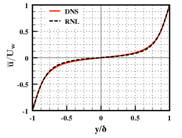
(a)

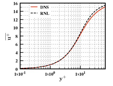
(b)

Figure 1: Turbulent mean velocity profiles (based on streamwise, spanwise and time averages) in (a) geometric units and (b) wall units obtained from DNS (red solid line) and unforced RNL simulations (black dashed line).

The turbulent mean velocity profile obtained from the DNS is compared to that obtained using the unforced RNL system in Figure 1a. Figure 1b provides a comparison of the same data in wall units, $u^{+}$ = $u/u_{\tau}$ and $y^{+}$ = $y\hskip 0.85358ptu_{\tau}/\nu$ with friction velocity $u_{\tau}$ = $\sqrt{\tau_{w}/\rho}$, $Re_{\tau}$ = $u_{\tau}\delta/\nu$ and $\nu$ = $1/R$. These wall unit values for the DNS results in Figure 1b are ${Re_{\tau}}$ = $66.2$ and ${u_{\tau}/U_{w}}$ = $6.62\times 10^{-2}$ and those corresponding to the RNL simulation are ${Re_{\tau}}$ = $64.9$ and ${u_{\tau}/U_{w}}$ = $6.49\times 10^{-2}$. Figure 1 illustrates good agreement between the turbulent mean velocity profile obtained from the RNL simulation and that obtained from the DNS, which is consistent with recent studies Farrell et al. (2012).

Instantaneous snapshots of the turbulent velocity fields from the DNS and the RNL simulation are displayed in Figures 2 and 3. Figure 2 shows contour plots of the $U$ velocity field with the $V$, $W$ vector fields superimposed. The large-scale roll structures characteristic of turbulent flow are evident in both simulations. Figure 3 illustrates the three-dimensional structure of the streamwise component of the velocity field. Figures 2 and 3 demonstrate that the DNS and the RNL system produce similar structures including comparable streak spacing and associated roll circulations. The visual similarity of the roll and streak structures produced by the DNS and RNL simulations implies that the RNL accurately captures these fundamental features of fully developed turbulent plane Couette flow.

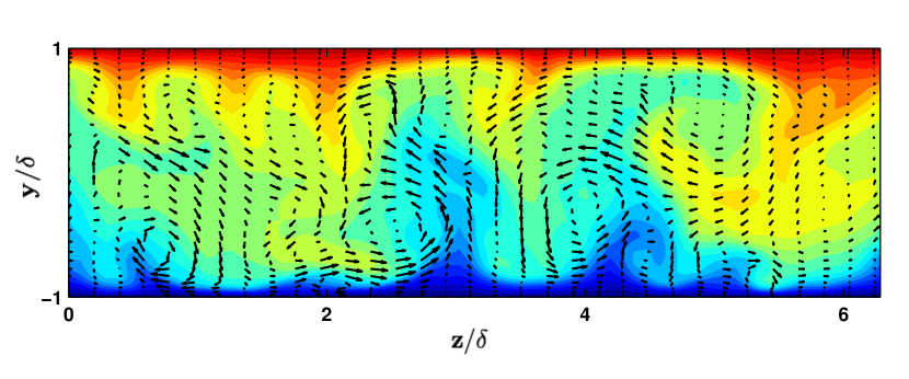
(a)  DNS

(b)  RNL

Figure 2: A $y$-$z$ plane cross-section of the streamwise constant structure (component $k_{x}$ = 0) of the flow at a single snapshot in time for a (a) DNS and a (b) RNL simulation. Both panels show contours of the streamwise component of the mean flow $U$ with the velocity vectors of ($V$,$W$) superimposed. The RNL is self-sustaining ($\mathbf{e}$ = 0) for the time shown

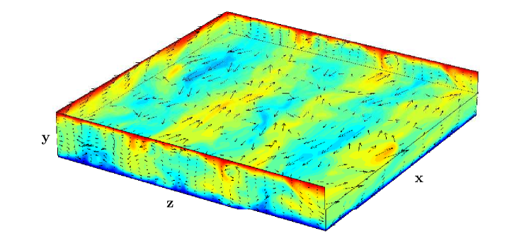
(a)  DNS

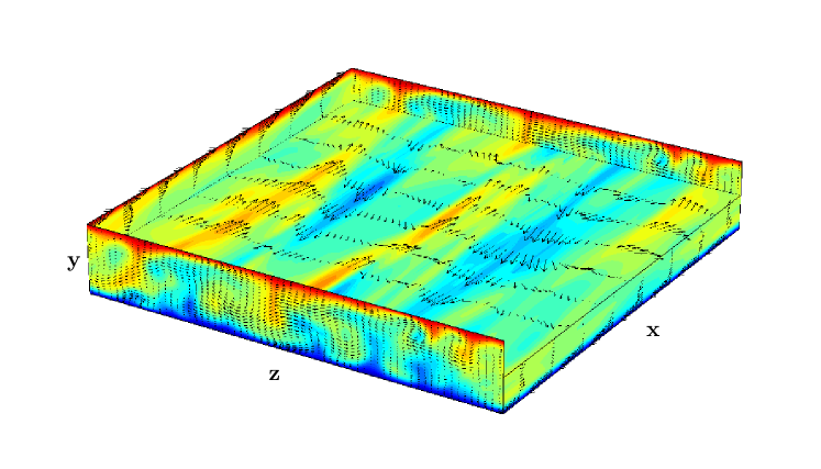
(b)

Figure 3: 3D perspective plots of the flow at a single snapshot in time for (a) a DNS, and (b) a RNL simulation Both images show contours of the streamwise component of the mean flow, $U$. The superimposed vectors represent the in-plane velocity vectors for the respective panel (i.e.: $(V,W)$ for the $y-z$ panels and $(U,W)$ for $x-z$ panels). The central $x-z$ panel shows the flow at the $y=0$ mid-plane of the system. The geometry of the systems are detailed in Table 1.

Figure 4 shows the corresponding time averaged Reynolds stresses, $\left[\overline{\langle u^{\prime+}u^{\prime+}\rangle}\right]$ and $\left[\overline{\langle u^{\prime+}v^{\prime+}\rangle}\right]$, where the streamwise fluctuations, $u^{\prime}$, are defined as $u^{\prime}$ = $u_{T}-\overline{u_{T}}$ and the wall-normal fluctuations , $v^{\prime}$, are defined as $v^{\prime}$ = $v_{T}-\overline{v_{T}}$. $u^{\prime+}$ and $v^{\prime+}$ designate these fluctuations scaled by $u_{\tau}$, such that $u^{\prime+}$ = $u^{\prime}/u_{\tau}$ and $v^{\prime+}$ = $v^{\prime}/u_{\tau}$. These figures illustrate close agreement between the $\overline{u^{\prime}v^{\prime}}$ Reynolds stress obtained from the RNL and DNS. However, the $\overline{u^{\prime}u^{\prime}}$ component has a higher magnitude in the RNL than in the DNS. As shown in Figure 1b, the turbulent flow supported by DNS and the RNL simulation exhibit nearly identical shear at the boundary. Therefore, the average energy input and by consistency the dissipation must be the same in these simulations. However, the RNL maintains a smaller number of streamwise Fourier components than the DNS Thomas et al. (2014). The result in Figure 4a is thus consistent with the smaller number of streamwise components supported by the RNL system producing the same dissipation as the DNS. This aspect of the dynamics is a subject of continuing investigation Thomas et al. (2014).

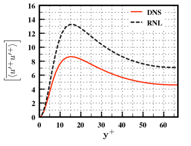
(a)

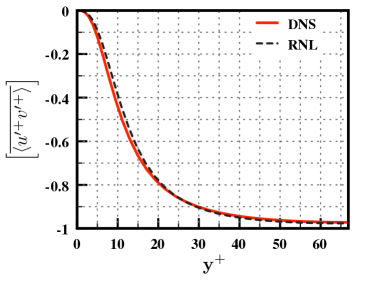
(b)

Figure 4: Reynolds stresses (a) $\left[\overline{\langle u^{\prime+}u^{\prime+}\rangle}\right]$ and (b) $\left[\overline{\langle u^{\prime+}v^{\prime+}\rangle}\right]$ obtained from a DNS and a RNL simulation. There is no stochastic excitation applied to the DNS or the RNL simulation during the time interval used to generate these profiles, (i.e. the RNL simulation is in the self-sustaining state)

Figures 5a and 5b shows close agreement in the root-mean-square (RMS) velocity departure from laminar, defined as $\sqrt{\left(\mathbf{U}+\mathbf{u}-\mathbf{U}_{\mathrm{lam}}\right)^{2}}$, and the RMS perturbation velocity, $\sqrt{u^{2}+v^{2}+w^{2}}$, between the RNL simulation and DNS. In particular, the RNL simulation maintains the same behavior after the initial forcing is removed (for $t>500$). In Figure 5c the friction Reynolds number, $Re_{\tau}$, is displayed as a function of dimensionless time, $u_{\tau}t/h$. The time interval in Figure 5c corresponds to $t\in[1000,6000]$, which verifies that the RNL system maintains turbulence for an extended interval of time. The RNL simulation thus exhibits both self-sustaining behavior and dissipation comparable to that in DNS.

The results shown in Figure 5 indicate that the self-sustaining behavior captured by the RNL system supports a SSP similar to that previously seen in the related S3T system Farrell and Ioannou (2012). Previous analysis of the S3T system established that this SSP is due to the coupling between the streamwise mean flow and the perturbations. In particular, the roll circulations are driven by the Reynolds stresses arising from the perturbations. Farrell and Ioannou (2012). In turn, maintenance of this perturbation field has been shown to result from a parametric non-normal growth process arising from the interaction between the time-dependent streak (resulting from the roll circulations) and the perturbation field Farrell and Ioannou (1996b, 1999, 2012). The similarity between the SSP operating in the S3T/RNL system with that in DNS provides evidence that the same mechanism underlies the SSP operating in these systems.

(a)

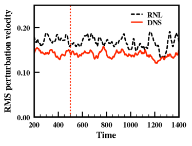
(b)

(c)

Figure 5: (a) RMS velocity minus laminar, $\sqrt{\left(\left(\mathbf{U}+\mathbf{u}\right)-\mathbf{U}_{\mathbf{lam}}\right)^{2}}$, (b) RMS perturbation velocity $\sqrt{u^{2}+v^{2}+w^{2}}$. The external excitation was stopped at $t=500$. The behavior of the RNL simulation for $t>500$ is similar to that of the DNS, indicating that the RNL simulation undergoes the SSP described in Farrell and Ioannou (2012), and (c) $Re_{\tau}$ versus dimensionless time, $u_{\tau}t/h$ obtained from DNS (red solid line) and the RNL (black dashed line) simulation. For DNS, $Re_{\tau}$ = $66.2$ and $u_{\tau}/U_{w}$ = $6.62\times 10^{-2}$. In the RNL simulation, ${Re_{\tau}}$ = $64.9$ and ${u_{\tau}/U_{w}}$ = $6.49\times 10^{-2}$

IV Comparison of RNL and 2D/3C Models

We now verify the fundamental role of the coupling between the mean flow equation (2a) and the perturbation equation (2b) in the maintenance of turbulence in the RNL system by comparing the RNL and 2D/3C models Gayme et al. (2010). The 2D/3C system can be obtained from (4) by replacing the time varying mean flow $\mathbf{U}$ in (4b) with the time-invariant laminar Couette flow $\mathbf{U}_{\mathbf{lam}}=U(y)$. The interaction whereby the mean flow influences the perturbations has thus been eliminated and the perturbation covariance evolves under stochastic forcing of the stable $A(\mathbf{U}_{\mathbf{lam}})$ for all times. In this case the mean flow dynamics represent a forced streamwise constant (2D/3C) system given by

$$\mathbf{U}\cdot\nabla\mathbf{U}+\nabla\mathbf{P}-\frac{1}{R}\Delta\mathbf{U}=-\mathcal{L}C^{\infty}$$ (5a)

$$\left(A_{1}(\mathbf{U}_{lam})+A_{2}(\mathbf{U}_{lam})\right)C^{\infty}=-Q~{},$$ (5b)

where $C^{\infty}$ denotes the asymptotic equilibrium covariance.

Figure 6a shows the same mean velocity profiles as in Figure 1a along with that obtained using a stochastically forced 2D/3C model Gayme et al. (2010). This plot demonstrates close correspondence between the mean velocity profiles obtained from DNS and simulations of the 2D/3C and RNL systems. Figure 6b shows the time evolution of the RMS streak velocity from simulations of the 2D/3C and RNL systems and DNS. Figure 6b shows that the streak in the 2D/3C model gradually decays to zero after the external excitation is removed at $t=500$. This figure demonstrates that a stochastically forced 2D/3C model captures the turbulent mean flow profile, but cannot maintain turbulence without stochastic excitation, see e.g. Bobba (2004).

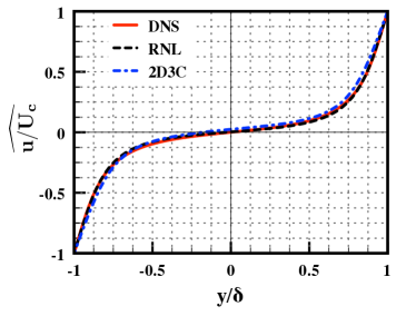
(a)

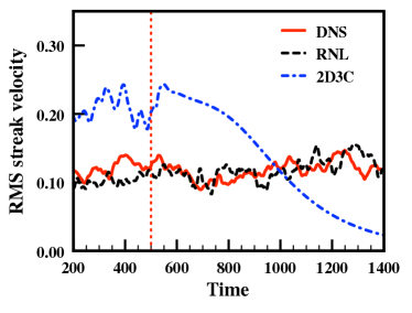
(b)

Figure 6: (a) Turbulent mean velocity profiles (based on a streamwise, spanwise and time averages) obtained from DNS (red solid line), and simulations of the RNL (black dashed line) and 2D/3C systems (blue dashed-dot line). There is no stochastic excitation applied to the DNS or the RNL simulation during the time interval used to generate the profile, whereas the 2D/3C simulation was continuously forced at $\mathbf{e}$ = 0.030. (b) The RMS streak velocity $\sqrt{U_{s}^{2}}$ obtained from DNS (red solid line) as well as the RNL (black dashed line) and 2D/3C simulations (blue dashed-dot line) where stochastic excitation was applied for $t\in[0,500]$, i.e., the excitation was stopped at $t=500$, which is indicated by the vertical red dotted line.

The critical difference between the 2D/3C and RNL systems is that the 2D/3C model lacks the interaction of the time-varying mean flow (2a) with the perturbation dynamics (2b). This difference is summarized by the block diagram in Figure 7. Both of these models include pathway ① in which the perturbations ($\mathbf{u}$) influence the dynamics of the mean flow ($\mathbf{U}$). However, the RNL system (and its associated ensemble mean S3T model) also includes the feedback pathway ②, from the mean flow to the perturbation dynamics. In Figure 6b the effect of this feedback from the mean flow to the perturbations, pathway ② in Figure 7, is seen to be critical for capturing the mechanism of the SSP maintaining the turbulent state. As shown in the previous section and in Figure 6, turbulence in the RNL system self-sustains (i.e., is maintained in the absence of stochastic excitation). Turbulence maintained by the same mechanism was seen previously in the S3T system in a minimal channel study Farrell and Ioannou (2012).

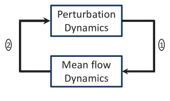
Figure 7: In both the 2D/3C and the unforced RNL model (2) (and its associated ensemble mean S3T model) the perturbations ($\mathbf{u}$) influence the dynamics of the mean flow ($\mathbf{U}$). This coupling is denoted pathway ① in the block diagram. The S3T model augments the 2D/3C formulation with feedback from the mean flow to the perturbation dynamics, which is illustrated through pathway ②.

In addition to being necessary to produce self-sustaining turbulence, the feedback from the mean flow to the perturbations produces streaks that are quantitatively and qualitatively similar to those observed in DNS, and notably more accurate than those obtained in the 2D/3C system. This result is consistent with the fact that in the 2D/3C model the streak is not regulated by feedback from the mean flow to the perturbation field, pathway ② in Figure 7. Therefore, understanding how the roll and streak structure and the mechanism by which it is maintained in a statistical steady state requires a model that includes feedback from the streamwise constant mean flow to the streamwise varying perturbation dynamics. Remarkably, only this additional feedback is required to capture the dynamics of the SSP, which both maintains the turbulent state and enforces its statistical equilibrium.

V Conclusions and directions for future work

In this work we have demonstrated that the RNL system, which models the dynamics of S3T, self-sustains turbulent activity. Comparisons between RNL simulations and the associated DNS demonstrate good agreement between the mean velocity fields and $uv$ component of the Reynolds stress with quantitative differences being confined to the $uu$ Reynolds stress component. The SSP supported by the RNL system is consistent with the familiar roll streak SSP observed in wall turbulence. The results discussed herein suggest that the SSP maintaining turbulence requires both the influence of the perturbations on the streamwise mean flow (captured in the 2D/3C mean flow model) and feedback from the mean flow to the streamwise varying perturbation field, which is additionally retained in the RNL model. Given that the RNL system restricts nonlinear coupling to that between the streamwise mean flow components and the perturbations, this agreement indicates that this highly restricted dynamics captures the fundamental mechanism of turbulence in plane Couette flow.

The RNL model shares the dynamical restriction of the S3T system and is obtained directly from the DNS by eliminating the perturbation-perturbation nonlinearity while retaining the mean-perturbation nonlinearities. It can therefore be seen as providing a bridge between S3T and DNS in which analytic insights gained using S3T can be directly related to DNS, which allows the mechanisms operating in these systems to be comprehensively compared. The structure of S3T leads to identification of an analytical SSP. This SSP is associated with the mechanism of streamwise streak forcing by roll circulations which are in turn maintained by perturbation Reynolds stresses Farrell and Ioannou (2012). Maintenance of the perturbation field in S3T has been shown to result from parametric non-normal interaction between the time-dependent streak and the perturbation field, see e.g. Farrell and Ioannou (1996b, 1999, 2012). Construction of the RNL system allows identification of this parametric non-normal SSP, which had been previously demonstrated to be operating in the S3T system, to be extended to DNS turbulence. The similarity between the SSP operating in the S3T/RNL system and that in DNS provides compelling evidence that the same mechanisms are operating in these systems. Continuing study of these models promises additional insight into the dynamics of turbulence in wall-bounded shear flows.

Acknowledgments

This work was initiated during the 2012 Center for Turbulence Research Summer Program with financial support from Stanford University and NASA Ames Research Center. We would like to thank Prof.  P. Moin and Prof. S. Lele for useful comments and fruitful discussions. Financial support from the National Science Foundation under CAREER Award CMMI-06-44793 (to M.R.J. and B.K.L.) and NSF AGS-1246929 and ATM-0736022 (to B.F.F) is gratefully acknowledged.

Appendix A

The operator $A(\mathbf{U})$ in (3) is obtained by taking the divergence of (2b) and using continuity (1c) and $\nabla\cdot\mathbf{e}=0$ to express the pressure as:

$$p=-\Delta^{-1}\left[\nabla\cdot\left(\mathbf{U}\cdot\nabla\mathbf{u}+\mathbf{u}\cdot\nabla\mathbf{U}\right)\right]~{},$$ (6)

so that

$${A}(\mathbf{U})\mathbf{u}=-\mathbf{U}\cdot\nabla\mathbf{u}-\mathbf{u}\cdot\nabla\mathbf{U}+\nabla\Delta^{-1}\left[\nabla\cdot\left(\mathbf{U}\cdot\nabla\mathbf{u}+\mathbf{u}\cdot\nabla\mathbf{U}\right)\right]+\frac{1}{R}\Delta\mathbf{u}~{}.$$ (7)

In the above, $\Delta^{-1}$ is the inverse of the Laplacian, rendered unique by imposition of the no slip boundary conditions at the channel walls.

As described in section II, the S3T system is a second order closure of the NS in (1), in which the first order cumulant is $\mathbf{U}$ and the second order nine component cumulant is the spatial covariance at time $t$ of the flow velocities $C\equiv C(1,2)=\langle\langle{\mathbf{u}_{1}\otimes\mathbf{u}_{2}}\rangle\rangle$ between the two points $\mathbf{x}_{1}=(x_{1},\,y_{1},\,z_{1})$ and $\mathbf{x}_{2}=(x_{2},\,y_{2},\,z_{2})$ where $\otimes$ is the tensor (outer) product Frisch (1995). The ensemble average over forcing realizations is denoted by $\langle\langle\cdot\rangle\rangle$, which under the ergodic assumption is equivalent to the streamwise average i.e. $\langle\langle\cdot\rangle\rangle\equiv\langle\cdot\rangle$. The flow then evolves according to (4), which is restated here for clarity:

$${\mathbf{U}_{t}}=\mathbf{U}\cdot\nabla\mathbf{U}+\nabla\mathbf{P}-\frac{1}{R}\Delta\mathbf{U}+\mathcal{L}C$$ (4a)

$${C_{t}}=\left(A_{1}(\mathbf{U})+A_{2}(\mathbf{U})\right)C+Q$$ (4b)

where $\mathbf{A}_{1}(\mathbf{U})C=\langle{\left(\mathbf{A}_{1}(\mathbf{U})\mathbf{u}_{1}\right)\otimes\mathbf{u}_{2}}\rangle$ indicates the contribution to the time rate of change of the covariance from the action of the operator $A(\mathbf{U})$, evaluated at point $\mathbf{x}_{1}$, on the corresponding component of $C$, and a similar relation holds for $\mathbf{A}_{2}(\mathbf{U})C$. $Q=\langle\langle\mathbf{e}_{1}\otimes\mathbf{e}_{2}\rangle\rangle$ is the second order covariance of the stochastic excitation under the assumption that the noise is temporally delta correlated. The mean equation (4a) is forced by the divergence of the perturbation Reynolds stresses $-\langle\mathbf{u}\cdot\nabla\mathbf{u}\rangle$ and this term can be expressed as a linear function of the covariance, $\mathcal{L}C$.

If (4a) is considered to be forced independently by a specified Reynolds stress divergence specified symbolically as $\mathcal{L}C$, then the mean flow dynamics (4a) define a forced streamwise constant or 2D/3C model of the flow field Bobba (2004); Gayme et al. (2010). The S3T system (4) is obtained by closing the dynamics through the coupling of the perturbation covariance evolution equation (4b) to the streamwise constant 2D/3C model.

References

- Kim, Moin, and Moser (1987) J. Kim, P. Moin, and R. Moser, “Turbulence statistics in fully developed channel flow at low Reynolds number,” J. Fluid Mech. 177, 133–166 (1987).
- Simens et al. (2009) M. Simens, J. Jimenez, S. Hoyas, and Y. Mizuno, “A high-resolution code for turbulent boundary layers,” J. Comp. Phys. 228, 4218–4231 (2009).
- del Álamo et al. (2004) J. C. del Álamo, J. Jiménez, Z. P., and M. R. D., “Scaling of the energy spectra of turbulent channels,” J. Fluid Mech. 500, 135–144 (2004).
- Tsukahara, Kawamura, and Shingai (2006) T. Tsukahara, H. Kawamura, and K. Shingai, “DNS of turbulent Couette flow with emphasis on the large-scale structure in the core region,” J. Turbulence 7 (2006).
- Hoyas and Jimenez (2008) S. Hoyas and J. Jimenez, “Reynolds number effects on the Reynolds-stress budgets in turbulent channels,” Phys. Fluids 20, 796–811 (2008).
- Farrell and Ioannou (1996a) B. F. Farrell and P. J. Ioannou, “Generalized stability. Part I: Autonomous operators,” J. Atmos. Sci. 53, 2025–2040 (1996a).
- Farrell and Ioannou (1996b) B. F. Farrell and P. J. Ioannou, “Generalized stability. Part II: Non-autonomous operators,” J. Atmos. Sci. 53, 2041–2053 (1996b).
- Farrell (1988) B. F. Farrell, “Optimal excitation of perturbations in viscous shear flow,” Phys. Fluids 31, 2093–2102 (1988).
- Gustavsson (1991) L. H. Gustavsson, “Energy growth of three-dimensional disturbances in plane Poiseuille flow,” J. Fluid Mech. 224, 241–260 (1991).
- Trefethen et al. (1993) L. N. Trefethen, A. E. Trefethen, S. C. Reddy, and T. A. Driscoll, “Hydrodynamic stability without eigenvalues,” Science 261, 578–584 (1993).
- Reddy and Henningson (1993) S. C. Reddy and D. S. Henningson, “Energy growth in viscous shear flows,” J. Fluid Mech. 252, 209–238 (1993).
- Farrell and Ioannou (1993a) B. F. Farrell and P. J. Ioannou, “Stochastic forcing of the linearized Navier-Stokes equations,” Phys. Fluids A 5, 2600–2609 (1993a).
- Bamieh and Dahleh (2001) B. Bamieh and M. Dahleh, “Energy amplification in channel flows with stochastic excitation,” Phys. Fluids 13, 3258–3269 (2001).
- Jovanović and Bamieh (2005) M. R. Jovanović and B. Bamieh, “Componentwise energy amplification in channel flows,” J. Fluid Mech. 534, 145–183 (2005).
- Henningson (1996) D. S. Henningson, “Comment on “Transition in shear flows. Nonlinear normality versus non-normal linearity” [Phys. Fluids 7, 3060 (1995)],” Phys. Fluids 8, 2257–2258 (1996).
- Henningson and Reddy (1994) D. S. Henningson and S. C. Reddy, “On the role of linear mechanisms in transition to turbulence,” Phys. Fluids 6, 1396–1398 (1994).
- Butler and Farrell (1993) K. M. Butler and B. F. Farrell, “Optimal perturbations and streak spacing in turbulent shear flow,” Phys. Fluids A 3, 774–776 (1993).
- Kim and Lim (2000) J. Kim and J. Lim, “A linear process in wall bounded turbulent shear flows,” Phys. Fluids 12, 1885–1888 (2000).
- Waleffe, Kim, and Hamilton (1991) F. Waleffe, J. Kim, and J. Hamilton, “On the origin of streaks in turbulent shear flows,” in Eighth Int’l Symposium on Turbulent Shear Flows (Munich, Germany, 1991).
- Jovanović and Bamieh (2001) M. R. Jovanović and B. Bamieh, “Modeling flow statistics using the linearized Navier-Stokes equations,” in Proc. of the 40th IEEE Conf. on Decision and Control (Orlando, FL, 2001) pp. 4944–4949.
- Jovanović and Georgiou (2010) M. R. Jovanović and T. T. Georgiou, “Reproducing second order statistics of turbulent flows using linearized Navier-Stokes equations with forcing,” in Bulletin of the American Physical Society (Long Beach, CA, 2010).
- Farrell and Ioannou (1998) B. F. Farrell and P. J. Ioannou, “Perturbation structure and spectra in turbulent channel flow,” Theor. Comput. Fluid Dyn. 11, 215–227 (1998).
- del Álamo and Jiménez (2006) J. C. del Álamo and J. Jiménez, “Linear energy amplification in turbulent channels,” J. Fluid Mech. 559, 205–213 (2006).
- Hwang and Cossu (2010) Y. Hwang and C. Cossu, “Amplification of coherent structures in the turbulent Couette flow: an input-output analysis at low Reynolds number,” J. Fluid Mech. 643, 333–348 (2010).
- Cossu, Pujals, and Depardon (2009) C. Cossu, G. Pujals, and S. Depardon, “Optimal transient growth and very large scale structures in turbulent boundary layers,” J. Fluid Mech. 619, 79–94 (2009).
- Moarref and Jovanović (2012) R. Moarref and M. R. Jovanović, “Model-based design of transverse wall oscillations for turbulent drag reduction,” J. Fluid Mech. 707, 205–240 (2012).
- Lumley (1967) J. L. Lumley, “The structure of inhomogeneous turbulence,” in Atmospheric Turbulence and Radio Wave Propagation, edited by A. M. Yaglom and V. I. Tatarskii (Nauka, Moscow, 1967) pp. 166–178.
- Smith, Moehlis, and Holmes (2005) T. R. Smith, J. Moehlis, and P. Holmes, “Low-dimensional modelling of turbulence using the proper orthogonal decomposition: A tutorial,” Nonlinear Dynamics 41, 275–307 (2005).
- Jiménez et al. (2005) J. Jiménez, G. Kawahara, M. P. Simens, M. Nagata, and M. Shiba, “Characterization of near-wall turbulence in terms of equilibrium and ‘bursting’ solutions,” Phys. Fluids 17, 015105 (2005).
- Kawahara, Uhlmann, and Van Veen (2012) G. Kawahara, M. Uhlmann, and L. Van Veen, “The significance of simple invariant solutions in turbulent flows,” Ann. Rev. Fluid Mech. 44, 203–225 (2012).
- Nagata (1990) M. Nagata, “Three-dimensional traveling-wave solutions in plane Couette flow,” J. Fluid Mech. 217, 519–527 (1990).
- Gibson, Halcrow, and Cvitanović (2009) J. F. Gibson, J. Halcrow, and P. Cvitanović, “Equilibrium and travelling-wave solutions of plane Couette flow,” J. Fluid Mech. 638, 243–266 (2009).
- Reynolds and Kassinos (1995) W. C. Reynolds and S. C. Kassinos, “One-point modelling of rapidly deformed homogeneous turbulence,” Proceedings of the Royal Society of London. Series A: Mathematical and Physical Sciences 451, 87–104 (1995).
- Bobba, Bamieh, and Doyle (2002) K. M. Bobba, B. Bamieh, and J. C. Doyle, “Highly optimized transitions to turbulence,” in Proc. of the IEEE Conf. on Decision and Control (Las Vegas, NV, 2002) pp. 4559–4562.
- Gayme et al. (2010) D. F. Gayme, B. J. McKeon, A. Papachristodoulou, B. Bamieh, and J. C. Doyle, “A streamwise constant model of turbulence in plane Couette flow,” J. Fluid Mech. 665, 99–119 (2010).
- Kim and Adrian (1999) K. J. Kim and R. J. Adrian, “Very large scale motion in the outer layer,” Phys. Fluids 11, 417–422 (1999).
- Guala, Hommema, and Adrian (2006) M. Guala, S. E. Hommema, and R. J. Adrian, “Large-scale and very-large-scale motions in turbulent pipe flow,” J. Fluid Mech. 554, 521–542 (2006).
- Hutchins and Marusic (2007) N. Hutchins and I. Marusic, “Evidence of very long meandering features in the logarithmic region of turbulent boundary layers,” J. Fluid Mech. 579, 1–28 (2007).
- McKeon and Sharma (2010) B. J. McKeon and A. S. Sharma, “A critical-layer framework for turbulent pipe flow,” J. Fluid Mech. 658, 336–382 (2010).
- Gayme et al. (2011) D. F. Gayme, B. J. McKeon, B. Bamieh, A. Papachristodoulou, and J. C. Doyle, “Amplification and nonlinear mechanisms in plane Couette flow,” Phys. Fluids 23, 065108 (2011).
- Bobba (2004) K. M. Bobba, Robust flow stability: Theory, computations and experiments in near wall turbulence, Ph.D. thesis, California Institute of Technology, Pasadena, CA, USA (2004).
- Note (1) A proof of this fact and the explicit construction of a Lyapunov function based on private communications with A. Papachristodoulou and B. Bamieh is provided in Gayme (2010).
- Farrell and Ioannou (2003) B. F. Farrell and P. J. Ioannou, “Structural stability of turbulent jets,” J. Atmos. Sci. 60, 2101–2118 (2003).
- DelSole and Farrell (1996) T. DelSole and B. F. Farrell, “The quasi-linear equilibration of a thermally mantained stochastically excited jet in a quasigeostrophic model,” J. Atmos. Sci. 53, 1781–1797 (1996).
- DelSole (2004) T. DelSole, “Stochastic models of quasigeostrophic turbulence,” Surveys in Geophysics 25, 107–194 (2004).
- Marston, Conover, and Schneider (2008) J. B. Marston, E. Conover, and T. Schneider, “Statistics of an unstable barotropic jet from a cumulant expansion,” J. Atmos. Sci. 65, 1955–1966 (2008).
- Tobias, Dagon, and Marston (2011) S. M. Tobias, K. Dagon, and J. B. Marston, “Astrophysical fluid dynamics via direct numerical simulation,” Astrophys. J. 727, 127 (2011).
- Srinivasan and Young (2012) K. Srinivasan and W. R. Young, “Zonostrophic instability,” J. Atmos. Sci. 69, 1633–1656 (2012).
- Farrell et al. (2012) B. F. Farrell, D. F. Gayme, P. Ioannou, B. Lieu, and M. R. Jovanović, “Dynamics of the roll and streak structure in transition and turbulence,” in Proc. of the Center for Turbulence Research Summer Program (2012) pp. 34–54.
- Kline et al. (1967) S. J. Kline, W. C. Reynolds, F. A. Schraub, and P. W. Runstadler, “The structure of turbulent boundary layers,” J. Fluid Mech. 30, 741–773 (1967).
- Landahl (1980) M. T. Landahl, “A note on an algebraic instability of inviscid parallel shear flows,” J. Fluid Mech. 98, 243 (1980).
- Swearingen and Blackwelder (1987) J. D. Swearingen and R. F. Blackwelder, “The growth and breakdown of streamwise vortices in the presence of a wall,” J. Fluid Mech. 182, 255–290 (1987).
- Blakewell and Lumley (1967) H. P. Blakewell and L. Lumley, “Viscous sublayer and adjacent wall region in turbulent pipe flow,” Phys. Fluids 10, 1880–1889 (1967).
- Waleffe (1995) F. Waleffe, “Hydrodynamic stability and turbulence:Beyond transients to a self-sustaining proccess,” Stud. Appl. Maths 95, 319–343 (1995).
- Hamilton, Kim, and Waleffe (1995) K. Hamilton, J. Kim, and F. Waleffe, “Regeneration mechanisms of near-wall turbulence structures,” J. Fluid Mech. 287, 317–348 (1995).
- Waleffe (1997) F. Waleffe, “On a self-sustaining process in shear flows,” Phys. Fluids A 9, 883–900 (1997).
- Hall and Sherwin (2010) P. Hall and S. Sherwin, “Streamwise vortices in shear flows: Harbingers of transition and the skeleton of coherent structures,” J. Fluid Mech. 661, 178–205 (2010).
- Schoppa and Hussain (2002) W. Schoppa and F. Hussain, “Coherent structure generation in near-wall turbulence,” J. Fluid Mech. 453, 57–108 (2002).
- Farrell and Ioannou (1993b) B. F. Farrell and P. J. Ioannou, “Optimal excitation of three dimensional perturbations in viscous constant shear flow,” Phys. Fluids 5, 1390–1400 (1993b).
- Farrell and Ioannou (2012) B. F. Farrell and P. J. Ioannou, “Dynamics of streamwise rolls and streaks in turbulent wall-bounded shear flow,” J. Fluid Mech. 708, 149–196 (2012).
- Jiménez (2013) J. Jiménez, “Near-wall turbulence,” Phys. Fluids 25, 101302 (2013).
- Gibson (2007) J. F. Gibson, “Channelflow: a spectral Navier–Stokes solver in C++,” Tech. Rep. (Georgia Institute of Technology, 2007).
- Peyret (2002) R. Peyret, Spectral Methods for Incompressible Flows (Springer-Verlag, 2002).
- Canuto et al. (1988) C. Canuto, M. Hussaini, A. Quateroni, and T. Zhang, Spectral Methods in Fluid Dynamics (Springer-Verlag, 1988).
- Zang and Hussaini (1985) T. A. Zang and M. Y. Hussaini, “Numerical experiments on subcritical transition mechanism,” in AIAA, Aerospace Sciences Meeting (Reno, NV, 1985).
- Thomas et al. (2014) V. Thomas, B. F. Farrell, D. F. Gayme, and P. Ioannou, “Structure and spectra of turbulence in an rnl plane couette flow,” In preparation (2014).
- Farrell and Ioannou (1999) B. F. Farrell and P. J. Ioannou, “Perturbation growth and structure in time dependent flows,” J. Atmos. Sci. 56, 3622–3639 (1999).
- Frisch (1995) U. Frisch, Turbulence: The Legacy of A. N. Kolmogorov (Cambridge University Press, 1995).
- Gayme (2010) D. F. Gayme, “A robust control approach to understanding nonlinear mechanisms in shear flow turbulence,” (2010).