On Coset Leader Graphs of LDPC Codes

Abstract

Our main technical result is that, in the coset leader graph of a linear binary code of block length $n$, the metric balls spanned by constant-weight vectors grow exponentially slower than those in $\{0,1\}^{n}$.

Following the approach of [1], we use this fact to improve on the first linear programming bound on the rate of LDPC codes, as the function of their minimal relative distance. This improvement, combined with the techniques of [2], improves the rate vs distance bounds for LDPC codes in a significant sub-range of relative distances.

1 Introduction

This paper deals with rate versus distance bounds for binary error-correcting codes.

A binary code $C$ of block length $n$, rate $R$, and relative minimal distance $\delta$ is a subset of $\{0,1\}^{n}$ of cardinality $2^{Rn}$, such that the Hamming distance between any two distinct elements of $C$ is at least $d=\delta n$. A fundamental open problem in coding theory is to find the largest possible asymptotic rate $R=R(\delta)$ for which there exists a family of codes $\left\{C_{n}\right\}_{n}$ with block length $n\rightarrow\infty$, rate at least $R$ and relative distance at least $\delta$.

The best known bounds on $R(\delta)$ are

$$1-H(\delta)\leq R(\delta)\leq R_{LP}(\delta)$$

The first inequality is the Gilbert-Varshamov bound [3]. Here $H(\cdot)$ is the binary entropy function. In the second inequality, we denote by $R_{LP}(\delta)$ the second JPL bound [4], obtained via the linear programming approach of Delsarte [5]. For an explicit expression for $R_{LP}(\delta)$ see e.g., [3].

Linear codes are an important subclass of error-correcting codes. A linear code of rate $R$ is an $Rn$-dimensional linear subspace of $\{0,1\}^{n}\cong\mathbb{F}^{n}_{2}$.

In this paper we consider a special class of linear codes. These are the Low-Density Parity Check (LDPC) codes. An LDPC code $C$ comes with an additional parameter - an absolute constant $w$. It has an additional structure: the dual code (dual subspace) $C^{\perp}$ is spanned by vectors of weight at most $w$.

LDPC codes were introduced by Gallager [6]. They are important both in theory and in practice of robust communications. A question of interest is to investigate the rate vs. minimal distance dependence in this class of codes. Let $R_{w}(\delta)$ be the largest possible asymptotic rate of an LDPC code whose dual is spanned by vectors of weight $w$ or less.

Gallager has shown that, for large $w$, LDPC codes reach the Gilbert-Varshamov bound, that is

$$\limsup_{w\rightarrow\infty}R_{w}(\delta)\geq 1-H(\delta)$$

From the other side, upper bounds on $R_{w}(\delta)$ were obtained in [7, 2]. These papers use the linear programming framework, combined with direct combinatorial and information-theoretic arguments exploiting the special structure of $C^{\perp}$, to improve on the second JPL bound $R_{LP}(\delta)$ for all values of $\delta$.

This paper continues the line of research started in [7, 2]. Our starting point is the elegant proof of the first JPL bound $R(\delta)\leq H(1/2-\sqrt{\delta(1-\delta)})$ for linear codes given in [1]. Given a linear code $C$, the strategy is to compare metric spaces defined on two graphs: the discrete cube $\{0,1\}^{n}$ and the coset leader graph $\mathbb{T}$ defined as the Cayley graph of the quotient group $\mathbb{F}_{2}^{n}/C^{\perp}$ with respect to the set of generators given by the standard basis $e_{1}\ldots e_{n}$. If $e_{i}+e_{j}\in C^{\perp}$, then edges in directions $i$ and $j$ are parallel and $\mathbb{T}$ becomes a multi-graph.

The name ’coset leader graph’ comes from a well-known notion in coding theory. Recall that a minimal weight element in a coset is called the coset leader [3]. (If the coset has more than one element of minimal weight, we take the coset leader to be minimal in the lexicographic order among them). This establishes a one-to-one correspondence between the vertices of $\mathbb{T}$ and coset leaders of $C^{\perp}$.

For a graph $G$, a vertex $x\in G$, and an integer parameter $r$, the metric ball $B(x,r)$ is the set of vertices whose distance from $x$ in the graph metric is at most $r$. We will be interested in the rate of growth of metric balls in $\mathbb{T}$. Since $\mathbb{T}$ is a vertex-transitive graph, we may choose the center arbitrarily, and we fix it to be the coset of zero. Accordingly, let $B_{\mathbb{T}}(r)$ be the metric ball $\left\{x\in\mathbb{T}~{}:d(x,C^{\perp})\leq r\right\}$. (Note that $B_{\mathbb{T}}(r)$ is the set of cosets with coset leader of Hamming weight at most $r$.) We are motivated by the following result of [1] restated in our own words.

Theorem 1.1

([1]): Let $C$ be a linear code with relative minimal distance $\delta$. Let $\mathbb{T}=\{0,1\}^{n}/C^{\perp}$ be the coset leader graph of $C^{\perp}$. Set $r=\left(\frac{1}{2}-\sqrt{\delta(1-\delta)}\right)\cdot n$. Then

$$|C|\leq 2^{o(n)}\cdot|B_{\mathbb{T}}(r)|$$

Our main technical result is that if $\mathbb{T}$ comes from an LDPC code, then the growth of metric balls in $\mathbb{T}$ is exponentially slower than that in $\{0,1\}^{n}$. Let $B(r)$ be the Hamming ball of radius $r$ in $\{0,1\}^{n}$ centered at zero. That is, $B(r)=\left\{x\in\{0,1\}^{n}~{}:|x|\leq r\right\}$, where $|\cdot|$ denotes the Hamming weight.

Theorem 1.2

: For any integer $w\geq 3$ and $0<\rho<1/2$, there is a constant $c=c(w,\rho)\geq\frac{\log_{2}e}{8w^{2}}\cdot\left(\frac{\rho^{w}}{2}\right)^{w+1}$ such that the following holds for any $n\geq w$:

Let $C\subseteq\{0,1\}^{n}$ be a linear code whose dual code $C^{\perp}$ is spanned by vectors of weight at most $w$, and let $\mathbb{T}=\{0,1\}^{n}/C^{\perp}$.

Then

$$|B_{\mathbb{T}}(\rho n)|\leq 2^{-cn}\cdot|B(\rho n)|.$$ (1)

Taken together with Theorem 1.1, this implies our main result. Recall that the first JPL bound is $R(\delta)\leq H\left(1/2-\sqrt{\delta(1-\delta)}\right)$. We improve this bound for $R_{w}(\delta)$.

Corollary 1.3

: For any $w\geq 3$,

$$R_{w}(\delta)\leq H\left(\frac{1}{2}-\sqrt{\delta(1-\delta)}\right)-c\left(w,~{}\frac{1}{2}-\sqrt{\delta(1-\delta)}\right)$$

where $c(w,\rho)$ is given by Theorem 1.2.

We give better estimates for $|B_{\mathbb{T}}(\rho n)|$ when $w=3$ and $w=4$, obtaining the following bounds for $R_{3}(\delta)$ and $R_{4}(\delta)$:

Theorem 1.4

: Let $0\leq\delta\leq\frac{1}{2}$. Then

$$R_{3}(\delta)\leq\left\{\begin{array}[]{lll}\rho+\frac{1}{2}H(2\rho)&\mbox{if}&\delta\geq\frac{1}{2}-\frac{\sqrt{2}}{3}\\ \frac{1}{3}+\frac{1}{2}H(1/3)&&\mbox{otherwise}\end{array}\right.$$

where $\rho=\frac{1}{2}-\sqrt{\delta(1-\delta)}$.

Theorem 1.5

: Let $0\leq\delta\leq\frac{1}{2}$. Then

$$R_{4}(\delta)\leq H(\rho)-\frac{\rho}{2}\cdot\log_{2}\left(\frac{1}{(1-\rho)^{4}+4\rho(1-\rho)^{3}+6\rho^{2}(1-\rho)^{2}}\right)$$

where $\rho=\frac{1}{2}-\sqrt{\delta(1-\delta)}$.

Remark 1.6

: The bound for $R_{3}(\delta)$ looks different from the one predicted by Corollary 1.3. The reason is that we have a particular way to upper bound the metric balls in $\mathbb{T}$ for $w=3$, which provides better bounds than Corollary 1.3.  

Comparing with Known Bounds

Our bound in Theorem 1.4 is better than the best known bounds for $R_{3}(\delta)$ [2], when $\delta$ is sufficiently close to $1/2$. However, we can do better. The argument in [2] holds if we replace the JPL bound it uses with our improved bound. This leads to a better bound on $R_{3}(\delta)$ for $0.156<\delta<0.5$.

The same line of argument leads to improved bounds on $R_{w}(\delta)$ for $0.287<\delta<0.5$, for any $w>3$. This range could probably be extended, but we do not attempt to do so in this paper.

Organization

We prove Theorem 1.2 in Section 2. Theorems 1.4 and 1.5 are proved in Sections 3 and 4 respectively. Comparison with known bounds is done in Section 5.

Notation

Throughout the paper, given a vector $v\in\{0,1\}^{n}$, we set $s(v)$ to be its support viewed as a subset of $\{1\ldots n\}$.

2 Proof of Theorem 1.2

Our first step reduces the problem to estimating a certain probability. Given $0<\rho<1/2$, let $x$ be a random vector in $\{0,1\}^{n}$, obtained by setting the coordinates independently to $1$ with probability $\rho=r/n$ and to $0$ with probability $1-\rho$. Let $p=p(\rho)$ be the probability that $x$ is a coset leader. In the following discussion we may, and will, assume $\rho n$ is an integer.

Lemma 2.1

:

$$p(\rho)\geq\Omega\left(\frac{1}{\sqrt{n}}\right)\cdot\frac{|B_{\mathbb{T}}(\rho n)|}{|B(\rho n)|}$$

Proof: Note that for $\rho<1/2$ the function $f(k)=\rho^{k}(1-\rho)^{n-k}$ decreases in $k$. Recall also that (by Stirling’s formula) $|B(\rho n)|\geq\Omega\left(\frac{1}{\sqrt{n}}\right)\cdot 2^{H(\rho)n}$. Therefore

$$p(\rho)\geq|B_{\mathbb{T}}(\rho n)|\cdot\rho^{\rho n}(1-\rho)^{n-\rho n}=|B_{\mathbb{T}}(\rho n)|\cdot 2^{-H(\rho)n}\geq\Omega\left(\frac{1}{\sqrt{n}}\right)\cdot\frac{|B_{\mathbb{T}}(\rho n)|}{|B(\rho n)|}$$

 

Hence, the claim of the theorem reduces to showing that there exists an absolute constant $c=c(w,\rho)\geq\frac{\log_{2}e}{8w^{2}}\cdot\left(\frac{\rho^{w}}{2}\right)^{w+1}$ such that $p<2^{-cn}$.

Let $v_{1},...,v_{m}$ be a basis of $C^{\perp}$ whose elements are vectors of Hamming weight at most $w$. Assume, w.l.o.g, that $\cup_{i=1}^{m}~{}s(v_{i})=\{1,\ldots,n\}$.

We partition the coordinates $\{1,\ldots,n\}$ into $w$ disjoint sets $I_{w},I_{w-1},\ldots I_{1}$, in the following way. Let $1\leq k\leq w$. Suppose $I_{w},I_{w-1}\ldots I_{k+1}$ are already defined, and let us define $I_{k}$. Initialize $I_{k}=\emptyset$. Go over the vectors $v_{i}$. If $s(v_{i})$ has exactly $k$ coordinates outside $I_{w}\cup I_{w-1}\cup\ldots\cup I_{k+1}\cup I_{k}$, add them to $I_{k}$.

Note that $|I_{k}|$ is always a multiple of $k$ (in particular $|I_{k}|$ can be zero). For instance, if $C^{\perp}$ is spanned by the vectors $v_{1}=\{1,1,1,0,0\}$, $v_{2}=\{0,0,1,1,0\}$ and $v_{3}=\{0,1,0,0,1\}$, then the partition is $I_{3}=\{1,2,3\}$, $I_{2}=\emptyset$ and $I_{1}=\{4,5\}$.

Lemma 2.2

: Let $A=\frac{2}{\rho^{w}}$. There exists an index $1\leq k\leq w$ such that

$$|I_{k}|>\max\left\{A\cdot\sum_{j=k+1}^{w}|I_{j}|,~{}\frac{n}{2wA^{w}}\right\}$$

Proof: If not, we will show that $|I_{k}|<\frac{n}{w}$ for all $1\leq k\leq w$, contradicting the fact that $|I_{1}|+|I_{2}|+\ldots+|I_{w}|=n$.

We note, for future reference, that $\rho<1/2$ implies $A>2^{w+1}$.

Let $S(k)$ stand for $A\cdot\sum_{j=k}^{w}|I_{j}|$. Note that our assumption is that for any $1\leq k\leq w$ holds

$$|I_{k}|\leq\max\left\{S(k+1),~{}\frac{n}{2wA^{w}}\right\}.$$

Since $S(1)=A\cdot n$ and $S(w+1)=0$, there exists an index $1\leq k_{0}\leq w$ such that $S(k_{0}+1)\leq\frac{n}{2wA^{w}}<S(k_{0})$.

We consider two cases, $k\geq k_{0}$ and $k<k_{0}$.

• $k\geq k_{0}$:

  This is the easy case. We have $S(k+1)\leq\frac{n}{2wA^{w}}$, and hence $|I_{k}|\leq\frac{n}{2wA^{w}}<\frac{n}{w}$. We record for later use that, in particular, $|I_{k_{0}}|\leq\frac{n}{2wA^{w}}$.

• $k<k_{0}$:

  We start with a few preliminary observations. First, in this case $\frac{n}{2wA^{w}}<S(k+1)$ and hence $|I_{k}|\leq S(k+1)$. This implies that $S(k)=A\cdot|I_{k}|+S(k+1)\leq(A+1)\cdot S(k+1)$.

  Next, we argue that $|I_{k}|\leq(A+1)^{k_{0}-k-1}\cdot S\left(k_{0}\right)$. This follows from the observations above, by applying the inequality $S(m)\leq(A+1)\cdot S(m+1)$ repeatedly for $m=k+1,...,k_{0}-1$.

  To complete the proof we need two more simple facts. Recall, that the definition of $k_{0}$ gives $S(k_{0}+1)\leq\frac{n}{2wA^{w}}$, and hence $S(k_{0})=A\cdot|I_{k_{0}}|+S(k_{0}+1)\leq(A+1)\cdot\frac{n}{2wA^{w}}$.

  Finally, note that since $A>2^{w+1}>w\geq 3$, we have $(A+1)^{w-1}<e\cdot A^{w-1}<A^{w}$. Putting everything together gives

  $$|I_{k}|<(A+1)^{k_{0}-k-1}\cdot S\left(k_{0}\right)\leq(A+1)^{w-2}\cdot S\left(k_{0}\right)\leq(A+1)^{w-1}\cdot\frac{n}{2wA^{w}}<\frac{n}{w}$$

 

Let $k$ be the index given by the lemma. Set $m=|I_{k}|$. Note that the coordinates of $I_{k}$ are divided into $t=m/k$ disjoint $k$-tuples $U_{1}\ldots U_{t}$ and each $U_{i}$ is contained in the support of a different basis element $v_{j_{i}}$. Note also that $s(v_{j_{i}})\setminus U_{i}$ is a subset of $\cup_{j=k+1}^{w}I_{j}$.

We claim that the support of any coset leader $x$ must contain at most $\frac{\rho^{k}}{2}\cdot t$ of the $k$-tuples $U_{i}$. Indeed, assume not and let $S\subset\{1\ldots t\}$ be the set of indices $i$ such that $U_{i}\subset s(x)$. Let $y=x+\sum_{i\in S}v_{j_{i}}$. Since $s(x)$ and $s(y)$ coincide on $I_{1}\cup I_{2}\cup\ldots\cup I_{k-1}$, we have

$$|y|\leq|x|-k\cdot|S|+\sum_{j=k+1}^{w}|I_{j}|<|x|-\frac{\rho^{k}}{2}\cdot|I_{k}|+\sum_{j=k+1}^{w}|I_{j}|<|x|$$

where the last inequality follows from the choice of $k$. Since $y$ belongs to the same coset as $x$, this contradicts the fact that $x$ is a coset leader.

Now, let $x$ be a random vector with coordinates set independently to $1$ with probability $\rho=r/n$ and to $0$ with probability $1-\rho$. Each $k$-tuple $U_{i}$ is in $s(x)$ with probability $\rho^{k}$ and the events of containing distinct tuples are statistically independent, since the tuples are disjoint. Let $p_{0}$ be the probability that $s(x)$ contains at most $\frac{\rho^{k}}{2}\cdot t$ of the tuples $U_{1}\ldots U_{t}$. By the preceding discussion, it upper bounds the probability $p$ that $x$ is a coset leader. Applying the Chernoff bound we have,

$$p\leq p_{0}\leq exp\left\{-\frac{\rho^{k}\cdot t}{8}\right\}$$

Recall that $t=\frac{|I_{k}|}{k}$. From Lemma 2.2, $|I_{k}|>\frac{n}{2wA^{w}}$. Hence,

$$\rho^{k}\cdot t=\frac{\rho^{k}}{k}\cdot\frac{|I_{k}|}{n}\cdot n\geq\frac{\rho^{w}}{w}\cdot\frac{1}{2wA^{w}}\cdot n=\frac{1}{w^{2}}\left(\frac{\rho^{w}}{2}\right)^{w+1}\cdot n$$

Hence $p\leq 2^{-cn}$ where $c=c(w,\rho)\geq\frac{\log_{2}e}{8w^{2}}\cdot\left(\frac{\rho^{w}}{2}\right)^{w+1}$, completing the proof of the theorem.

3 Proof of Theorem 1.4

In this section we treat the case $w=3$. We present a simple argument to bound the growth of metric balls in the coset leader graph $\mathbb{T}$, which does better in this special case than the more general approach of Theorem 1.2. Unfortunately, we were not able to extend it to larger values of $w$.

We will argue that for any distance $r$ attainable in $\mathbb{T}$, an element $x+C^{\perp}$ which belongs to the $r$-sphere $S_{r}=S_{\mathbb{T}}(r)$ around zero has at most $n-2r$ neighbours in the next sphere $S_{r+1}$. This should be compared to the situation in the Hamming cube, in which an element in the $r$-sphere has $n-r$ neighbours in the $(r+1)$-sphere. A simple calculation will then show that the metric balls in the coset leader graph grow much slower than in the cube, and prove the claim of the theorem.

In the following discussion we assume w.l.o.g. that $\cup_{v\in C^{\perp},|v|\leq 3}s(v)=\{1,\ldots,n\}$.

Consider an element $x+C^{\perp}\in S_{r}$. Assume $x$ is the coset leader, in particular $|x|=r$. For each coordinate $i\in s(x)$ let $v_{i}\in C^{\perp}$ be a vector of weight at most $3$ whose support contains $i$. The key point in the argument is that there are at least $2r$ directions to go from $x+C^{\perp}$ that do not lead away from zero. This is shown in the following lemma.

Lemma 3.1

:

1. For all $j\in\cup_{i\in s(x)}s(v_{i})\quad\mbox{holds}\quad d\left(0,x+e_{j}+C^{\perp}\right)\leq r$

2. $\Big{|}\cup_{i\in s(x)}s(v_{i})\Big{|}\,\geq\,2r\quad\mbox{ (in particular $r\leq n/2$)}$

Proof: First note that $s(x)\subseteq\cup_{i\in s(x)}s(v_{i})$. Let $j\in\cup_{i\in s(x)}s(v_{i})$. We distinguish between two cases. If $j\in s(x)$, the element $(x+e_{j})+C^{\perp}$ is in $S_{r-1}$. For $j\not\in s(x)$, let $j\in s(v_{i})$ for some $i\in s(x)$. The vector $x+e_{j}+v_{i}$ is of weight at most $r$, since $i\in s(x)$ , $j\in s(v_{i})$, and $i\not=j$. Therefore $d\left(0,x+e_{j}+C^{\perp}\right)\leq r$.

It remains to show $\Big{|}\cup_{i\in s(x)}s(v_{i})\Big{|}\geq 2r$.

Let $z=\sum_{i\in s(x)}v_{i}$. We will show that $|z|\geq 2r$, which will give what we want, since $z$ is supported in $\cup_{i\in s(x)}s(v_{i})$. Observe that for all $i\in s(x)$ holds $s(v_{i})\cap s(x)=\{i\}$, since otherwise $y=x+v_{i}$ would be a smaller weight element in the same coset. Hence $s(x)\subseteq s(z)$, which implies $|z|\geq 2r$. Indeed, if not, we would have $|x+z|=|z|-|x|<r$, and $y=x+z$ would be a smaller weight element in the coset of $x$.  

We now use this to bound the rate of growth of metric spheres in $\mathbb{T}$. Consider the bipartite graph whose parts are given by $S_{r}$ and $S_{r+1}$ and two vertices are connected if they are neighbours in $\mathbb{T}$. We have shown that the degree of any element in $S_{r}$ is at most $n-2r$. On the other hand, the degree of every element in $S_{r+1}$ is, obviously, at least $r+1$. By a standard double counting argument, this implies

$$|S_{r+1}|\leq\frac{n-2r}{r+1}\cdot|S_{r}|$$

Therefore, for $r\leq n/2$ holds

$$|S_{r}|\leq\frac{1}{r!}\cdot\prod_{k=0}^{r-1}(n-2k)\leq 2^{r}\cdot\binom{\lceil n/2\rceil}{r}$$

and, obviously, $S_{r}=0$ for larger $r$.

The expression $2^{r}\cdot\binom{\lceil n/2\rceil}{r}$ increases in $r$ till $r=\lceil n/3\rceil$ and decreases for larger $r$. Therefore (omitting integer rounding for the sake of typographic clarity)

$$|B_{\mathbb{T}}(r)|~{}~{}=~{}~{}\sum_{k=0}^{r}|S_{k}|\quad<\quad\left\{\begin{array}[]{ll}n\cdot 2^{r}\cdot\binom{n/2}{r}&\hbox{if $r\leq n/3$;}\\ n\cdot 2^{n/3}\cdot\binom{n/2}{n/3}&\hbox{if $r>n/3$.}\end{array}\right.$$

Substituting $r=\rho n$ and using the inequality $\binom{n}{\rho n}\leq 2^{nH(\rho)}$, we obtain

$$|B_{\mathbb{T}}(\rho n)|\leq\left\{\begin{array}[]{ll}2^{n\left(\rho+\frac{1}{2}H(2\rho)\right)}&\hbox{if $\rho\leq 1/3$;}\\ 2^{n\left(\frac{1}{3}+\frac{1}{2}H(2/3)\right)}&\hbox{if $\rho>1/3$.}\end{array}\right.$$ (2)

The proof of Theorem 1.4 is completed by using this bound in Theorem 1.1.  

4 Proof of Theorem 1.5

We deduce the theorem from Theorem 1.1 by showing that $|B_{\mathbb{T}}(\rho n)|\leq 2^{-cn}\cdot|B(\rho n)|$ where

$$c=c(\rho)\geq\frac{\rho}{2}\cdot\log_{2}\left(\frac{1}{(1-\rho)^{4}+4\rho(1-\rho)^{3}+6\rho^{2}(1-\rho)^{2}}\right)-o_{n}(1)$$ (3)

Let $I_{1},I_{2},I_{3},I_{4}$ be the partition of $[n]$ , as defined in the proof of Theorem 1.2. Let

$$|I_{1}|=\alpha_{1}n,\quad|I_{2}|=\alpha_{2}n,\quad|I_{3}|=\alpha_{3}n,\quad|I_{4}|=\alpha_{4}n$$

Note that $\alpha_{1}+\alpha_{2}+\alpha_{3}+\alpha_{4}=1$.

The following lemma shows existence of elements of prescribed structure in each coset of $C^{\perp}$. Both the statement and the proof of the lemma refer to the properties of the partition $\{I_{j}\}$, as described in the proof of Theorem 1.2.

Lemma 4.1

: Let $u\in\{0,1\}^{n}$.

1. There is an element $u_{1}\in u+C^{\perp}$ whose support does not intersect $I_{1}$.

2. There is an element $u_{2}\in u+C^{\perp}$ whose weight is at most that of $u$ and such that

   • $s(u_{2})\cap I_{1}=s(u)\cap I_{1}$.

   • $s(u_{2})$ intersects each $j$-tuple of $I_{j}$ in a most $\lfloor j/2\rfloor$ coordinates for $j=2,3,4$.

Before proving the lemma, we state two corollaries.

Corollary 4.2

:

1. Each coset of $C^{\perp}$ has a representative whose support intersects each $j$-tuple of $I_{j}$ in a most $\lfloor j/2\rfloor$ coordinates for $j=1,2,3,4$.

2. Each coset of $C^{\perp}$ has a minimal weight representative whose support intersects each $j$-tuple of $I_{j}$ in a most $\lfloor j/2\rfloor$ coordinates for $j=2,3,4$.

Proof:

1. Apply both parts of the lemma to any element $u$ in the coset.

2. Apply the second part of the lemma to a minimal weight element $u$ in the coset.

 

Corollary 4.3

: The diameter of the coset leader graph $\mathbb{T}=\{0,1\}^{n}/C^{\perp}$ is at most $D=\left(\alpha_{2}/2+\alpha_{3}/3+\alpha_{4}/2\right)\cdot n$.

Proof:

Since $\mathbb{T}$ is vertex-transitive, it suffices to show that the distance of any coset of $C^{\perp}$ from zero is at most $D$. To see this, note that each coset has a representative whose structure is given by the first part of Corollary 4.2. It is immediate that its weight is at most $D$.  

Proof of Lemma 4.1

The first part of the lemma. For each coordinate $i\in I_{1}$ contained in the support of $u$, add to $u$ a basis vector $v_{i}\in C^{\perp}$ whose support intersects $I_{1}$ only in this coordinate. Such a vector exists from the definition of $I_{1}$. This process terminates in an element $u_{1}$ in the same coset, whose support does not intersect $I_{1}$.

The second part of the lemma. We modify $u$ in three steps, by adding vectors from $C^{\perp}$, until we arrive to the required structure. We keep track of the weight of $u$ to see that it does not increase in the process.

1. For each pair $(i,j)$ in $I_{2}$ contained in the support of $u$, add to $u$ a basis vector $v\in C^{\perp}$ of weight at most four whose support contains $(i,j)$, and whose remaining elements are in $I_{3}\cup I_{4}$. Note that this does not increase the weight of $u$ and does not change its intersection with $I_{1}$. At the end of this step we obtain an element $u^{\prime}\in u+C^{\perp}$ whose support intersects each pair of $I_{2}$ in at most one coordinate.

2. For each triple in $I_{3}$ that intersects the support of $u^{\prime}$ in at least two coordinates, add to $u^{\prime}$ a basis vector $v\in C^{\perp}$ of weight at most four whose support contains this triple, and whose remaining element (if it exists) is in $I_{4}$. This does not increase the weight of $u^{\prime}$ and does not change its intersection with $I_{1}$ and $I_{2}$. This step terminates at an element $u^{\prime\prime}$ of the same coset intersecting $I_{1}$, $I_{2}$ and $I_{3}$ as required.

3. For each $4$-tuple in $I_{4}$ that intersects the support of $u^{\prime\prime}$ in more than two coordinates, add it to $u^{\prime\prime}$. This does not increase the weight of $u^{\prime\prime}$ and does not change its intersection with $I_{1}$, $I_{2}$, and $I_{3}$. At the end of the process we obtain an element $u_{2}\in u+C^{\perp}$ intersecting all $I_{j}$ as required.

 

We proceed towards the proof of (3). By Corollary 4.3, it suffices to deal with $0\leq\rho\ \leq\frac{\alpha_{2}}{2}+\frac{\alpha_{3}}{3}+\frac{\alpha_{4}}{2}$. Let us fix such $\rho$.

Let $x$ be a random vector in $\{0,1\}^{n}$, obtained by setting the coordinates independently to $1$ with probability $\rho=r/n$ and to $0$ with probability $1-\rho$. Let $p=p(\rho)$ be the probability that $x$ is a coset leader. By Lemma 2.1 it is enough to show $p(\rho)\leq 2^{-cn}$ where $c$ is given by the RHS of (3).

Let $p^{\prime}=p^{\prime}(\rho)$ be the probability that $x$ is of minimal weight in its coset and has the structure prescribed by the second part of Corollary 4.2. Note that each coset has exactly one coset leader and at least one element with the properties given in the corollary. Therefore $p\leq p^{\prime}$. In the remaining part of the proof we show that $p^{\prime}\leq 2^{-cn}$.

Corollary 4.2 imposes $\left(\frac{\alpha_{2}}{2}+\frac{\alpha_{3}}{3}+\frac{\alpha_{4}}{4}\right)\cdot n$ statistically independent constraints on $x$. The probability for all of them to hold is

$$\left((1-\rho)^{4}+4\rho(1-\rho)^{3}+6\rho^{2}(1-\rho)^{2}\right)^{\frac{1}{4}\alpha_{4}n}\cdot\left((1-\rho)^{3}+3\rho(1-\rho)^{2}\right)^{\frac{1}{3}\alpha_{3}n}\cdot\left(1-\rho^{2}\right)^{\frac{1}{2}\alpha_{2}n}$$ (4)

Recall that $\rho\leq\alpha_{2}/2+\alpha_{3}/3+\alpha_{4}/2$. Hence, $p^{\prime}(\rho)$ is bounded from above by the maximum value the expression in (4) attains in the domain

$$\Delta(\rho)=\Big{\{}\alpha_{1},\alpha_{2},\alpha_{3},\alpha_{4}\geq 0,\quad\alpha_{1}+\alpha_{2}+\alpha_{3}+\alpha_{4}=1,\quad\alpha_{2}/2+\alpha_{3}/3+\alpha_{4}/2\geq\rho\Big{\}}$$

We claim that for fixed $\alpha_{1}$, this expression is maximized when $\alpha_{2}=\alpha_{3}=0$ and $\alpha_{4}=1-\alpha_{1}$. To see this, we start with a technical lemma:

Lemma 4.4

: For any $0\leq\rho\leq 1/2$,

$$\left((1-\rho)^{4}+4\rho(1-\rho)^{3}+6\rho^{2}(1-\rho)^{2}\right)^{\frac{1}{4}}\geq\max\left\{\left((1-\rho)^{3}+3\rho(1-\rho)^{2}\right)^{\frac{1}{3}},\left(1-\rho^{2}\right)^{\frac{1}{2}}\right\}$$

Proof: Dividing out by $(1-\rho)^{1/2}$ and rearranging, it suffices to show:

$$\left((1+\rho)^{2}+2\rho^{2}\right)^{1/4}\geq\left(1+\rho\right)^{1/2}\geq(1-\rho)^{1/6}(1+2\rho)^{1/3}$$

The first inequality is immediate. For the second inequality, observe that

$$(1+\rho)^{3}-(1-\rho)(1+2\rho)^{2}=5\rho^{3}+3\rho^{2}\geq 0$$

 

By the lemma, increasing $\alpha_{4}$ and decreasing $\alpha_{2}+\alpha_{3}$ by the same amount increases (4) and leaves us in $\Delta(\rho)$ as long as $\alpha_{2},\alpha_{3}\geq 0$. Consequently, we may take $\alpha_{2}=\alpha_{3}=0$ and $\alpha_{4}=1-\alpha_{1}$.

We arrive to the problem of maximizing $\left((1-\rho)^{4}+4\rho(1-\rho)^{3}+6\rho^{2}(1-\rho)^{2}\right)^{\frac{1}{4}\alpha_{4}n}$ on $[2\rho,1]$.

Since $(1-\rho)^{4}+4\rho(1-\rho)^{3}+6\rho^{2}(1-\rho)^{2}<1$, the maximum is attained at $\alpha_{4}=2\rho$. Hence

$$p^{\prime}\leq\left((1-\rho)^{4}+4\rho(1-\rho)^{3}+6\rho^{2}(1-\rho)^{2}\right)^{\frac{1}{2}\rho n},$$

concluding the proof of (3).

5 Comparison to Other Bounds

Ben Haim and Litsyn [2], (see also [7]) give the best known upper bounds on the rate of LDPC codes with relative minimal distance $\delta$:

$$R(C) \leq R_{w}^{(1)}(\delta) =1-\frac{H(\delta/2)}{H((1-(1-\delta)^{w})/2)}$$ (5)

$$R(C) \leq R_{w}^{(2)}(\delta) =1-\max_{\delta/2\leq u\leq 1/2}\left(\frac{H(u)-R_{cw}(u,\delta)}{H((1-(1-2u)^{w})/2)}\right)$$ (6)

$$R(C) \leq R_{w}^{(4)}(\delta) =\min_{0\leq t\leq 1-2\delta}\left((1-t)R_{LP}(\delta/(1-t))+t-\frac{t}{w}\right)$$ (7)

$$R(C) \leq R_{w}^{(5)}(\delta) =\min_{0\leq t\leq 1-2\delta}\left((1-t)R_{LP}(\delta/(1-t))+t-\frac{t}{w-1}\right)$$ (8)

where $R_{w}^{(1)}(\delta)$, $R_{w}^{(2)}(\delta)$, $R_{w}^{(4)}(\delta)$, and $R_{w}^{(5)}(\delta)$ are the bounds in Theorems 1, 2, 4 and 5 respectively of [2]. Let us mention that the bound $R_{w}^{(5)}(\delta)$ requires an additional assumption, namely that the weight of each column in the parity check matrix is at least two.

5.1 The Case $w=3$

Figure 1 presents several bounds for the case $w=3$.

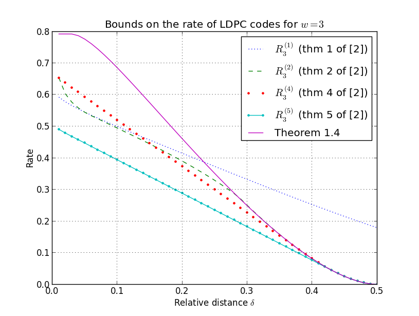
Figure 1: The bound in Theorem 1.4 and the bounds of [2]

We start with a comparison between the different bounds from [2]. The bound $R_{3}^{(5)}$ is better than the others for the whole range $0\leq\delta\leq 0.5$. However, it requires the additional assumption that the weight of each column in the parity matrix is at least 2. Without this assumption, we are left with the bounds $R_{3}^{(1)}$, $R_{3}^{(2)}$ and $R_{3}^{(4)}$, each of which is optimal in a subrange of $0\leq\delta\leq 0.5$.

Our bound in Theorem 1.4 is better than $R_{3}^{(4)}$ for $\delta>0.3877$ and better than $R_{3}^{(5)}$ for $\delta>0.4387$, since for these values of $\delta$ those two bounds coincide with the first JPL bound, and the bound in Theorem 1.4 is always better than the first JPL bound.

With that, we can do better. The argument in Theorems 4 and 5 in [2] holds if we replace the second JPL bound they use with the better bound of Theorem 1.4 (since the first and the second JPL bounds coincide at the optimal values of $t$ in (7) and (8)). This leads to a (small) improvement on $R_{3}^{(4)}$ and $R_{3}^{(5)}$, and hence to best known bounds when these two bounds are optimal. ($R_{3}^{(4)}$ is optimal for $0.156<\delta<1/2$).

To sum up, we improve the bounds on $R_{3}(\delta)$ for $0.156<\delta<1/2$. Given the additional assumption that the weight of each column in the parity check matrix is at least 2, we improve the bounds on the rate for the whole range $0<\delta<0.5$.

5.2 The Case $w>3$

In this subsection, for brevity’s sake, we deal only with bounds on $R_{w}(\delta)$, with no additional assumptions on the weight of the columns in the parity check matrix. Consider the subrange of the interval $0<\delta<0.5$ in which the following two conditions hold. The bound $R_{w}^{(4)}(\delta)$ of [2] is better than $R_{w}^{(1)}(\delta)$ and $R_{w}^{(2)}(\delta)$, and in addition to this, the first and the second JPL bounds coincide at the optimal values of $t$ in (7). In this subrange, similarly to the case $w=3$, we can use Corollary 1.3 or Theorem 1.5 to improve on $R_{w}^{(4)}(\delta)$, and hence on $R_{w}(\delta)$.

We proceed by comparing the three bounds from [2]. For this purpose, we first compare them to the second JPL bound:

• $R_{w}^{(1)}(\delta)$:

  Numerical calculations show that $R_{3}^{(1)}(\delta)$ is bigger than the second JPL bound for $\delta>0.23$. Since $R_{w}^{(1)}(\delta)$ increases with $w$, this holds for all $w\geq 3$.

• $R_{w}^{(2)}(\delta)$:

  Numerical calculations show that $R_{3}^{(2)}(\delta)$ equals to the second JPL bound for $\delta>0.287$. Since $R_{w}^{(2)}(\delta)$ increases with $w$, it is at least as large as the second JPL bound for all $w\geq 3$ in this range.

• $R_{w}^{(4)}(\delta)$:

  Substituting $t=0$ in the RHS of (7) recovers the second JPL bound. Hence $R_{w}^{(4)}(\delta)$ is at most as large as the second JPL bound for all $w\geq 3$.

To sum up: For $\delta>0.287$, $R_{w}^{(4)}(\delta)$ is at least as good as the other two bounds, for all $w\geq 3$. Next, note that in this range, the first and the second JPL bounds coincide at all values of $t$ in (7), since they coincide on the interval $0.273\leq\delta\leq 0.5$. Hence, we improve the bounds of [2] in this range.

References

- [1] J. Friedman and J.-P. Tillich, “Generalized Alon-Boppana theorems and error-correcting codes,” SIAM J. Discrete Math., vol. 19, no. 3, pp. 700–718 (electronic), 2005.
- [2] Y. Ben-Haim and S. Litsyn, “Upper bounds on the rate of LDPC codes as a function of minimum distance,” IEEE Trans. Inform. Theory, vol. 52, no. 5, pp. 2092–2100, 2006.
- [3] F. J. MacWilliams and N. J. A. Sloane, The theory of error-correcting codes. North-Holland Publishing Co., Amsterdam-New York-Oxford, 1977. North-Holland Mathematical Library, Vol. 16.
- [4] R. J. McEliece, E. R. Rodemich, H. Rumsey, Jr., and L. R. Welch, “New upper bounds on the rate of a code via the Delsarte-MacWilliams inequalities,” IEEE Trans. Information Theory, vol. IT-23, no. 2, pp. 157–166, 1977.
- [5] P. Delsarte, “An algebraic approach to the association schemes of coding theory,” Philips Res. Rep. Suppl., no. 10, pp. vi+97, 1973.
- [6] R. Gallager, “Low-density parity-check codes,” MIT press, 1963.
- [7] D. Burshtein, M. Krivelevich, S. Litsyn, and G. Miller, “Upper bounds on the rate of LDPC codes,” IEEE Trans. Inform. Theory, vol. 48, no. 9, pp. 2437–2449, 2002.