Molecules, dust, and protostars in NGC 3503

Abstract

Aims. We are presenting here a follow-up study of the molecular gas and dust in the environs of the star forming region NGC 3503. This study aims at dealing with the interaction of the Hii  region NGC 3503  with its parental molecular cloud, and also with the star formation in the region, that was possibly triggered by the expansion of the ionization front against the parental cloud.

Methods. To analyze the molecular gas we use CO(J=2$\rightarrow$1), ¹³CO(J=2$\rightarrow$1), C¹⁸O(J=2$\rightarrow$1), and HCN(J=3$\rightarrow$2) line data obtained with the on-the-fly technique from the APEX telescope. To study the distribution of the dust, we make use of unpublished images at 870 $\mu$m from the ATLASGAL survey and IRAC-GLIMPSE archival images. We use public 2MASS and WISE data to search for infrared candidate YSOs in the region.

Results. The new APEX observations allowed the substructure of the molecular gas in the velocity range from $\sim$ $-$28 to $-$23 km s^-1 to be imaged in detail. The morphology of the molecular gas close to the nebula, the location of the PDR, and the shape of radio continuum emission suggest that the ionized gas is expanding against its parental cloud, and confirm the “champagne flow” scenario. We have identified several molecular clumps and determined some of their physical and dynamical properties such as density, excitation temperature, mass, and line width. Clumps adjacent to the ionization front are expected to be affected by the Hii  region, unlike those that are distant to it. We have compared the physical properties of the two kind of clumps to investigate how the molecular gas has been affected by the Hii  region. Clumps adjacent to the ionization fronts of NGC 3503 and/or the bright rimmed cloud SFO 62  have been heated and compressed by the ionized gas, but their line width is not different to those that are too distant to the ionization fronts. We identified several candidate YSOs in the region. Their spatial distribution suggests that stellar formation might have been boosted by the expansion of the nebula. We discard the “collect and collapse” scenario and propose alternative mechanisms such as radiatively driven implosion on pre-existing molecular clumps or small-scale Jeans gravitational instabilities.

1 Introduction

It is accepted that OB associations have an enormous impact on the state of their environs. The interstellar medium (ISM) surrounding OB stars is expected to be strongly modified and disturbed by their intense ultraviolet (UV) radiation field ($h\nu>$ 13.6 eV). UV photons ionize the surrounding gas creating Hii  regions and dissociate the molecular gas originating photodissociation regions (PDRs) (Hollenbach & Tielens, 1997). Further, the surrounding neutral gas (either atomic or molecular), is compressed by the expansion of the Hii  region and/or the action of stellar winds. The compression of the cloud could enhance the stellar formation via “radiative driven implosion” process (RDI; Lefloch & Lazareff 1994) or even trigger it via “collect and collapse” process (Elmegreen & Lada, 1977). Therefore, when massive stars form inside a molecular cloud it is expected that they dominate the state of the parental cloud and consequently the further stellar formation process within. Indeed, it has been shown that a large fraction of stars originates at the peripheries of Hii regions (Pomarès et al., 2009; Romero & Cappa, 2009; Cappa et al., 2009; Deharveng et al., 2010; Vasquez et al., 2012; Deharveng et al., 2012). Having this in mind, it is instructive to study the molecular gas adjacent to Hii regions since it can provide important information on the interaction between massive stars and their natal environments. Furthermore, a comparison between regions of the molecular cloud adjacent to an Hii region with other sites away from it may provide significant understanding into the physical properties of the molecular gas that may impact the formation of stars.

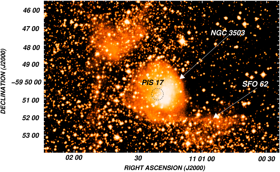
Figure 1: UKST red plate image of the nebula NGC 3503 in the area covered by the APEX data. The positions of NGC 3503, the bright rimmed cloud SFO 62 , and the open cluster Pis 17 are indicated.

The optical emission nebula NGC 3503 (= Hf 44 = BBW 335) is a small Hii region located at RA, Dec. (J2000) = (11^h01^m16^s, $-$59^∘50′39″) (Dreyer & Sinnott, 1988), and placed at a distance of 2.9 $\pm$ 0.4 kpc (Pinheiro et al., 2010). NGC 3503  is ionized by early B-type stars belonging to the open cluster Pis 17 (Herbst, 1975; Pinheiro et al., 2010; Duronea et al., 2012) and is believed to be related to the bright-rimmed cloud (BRC) SFO 62 (Sugitani et al., 1991; Yamaguchi et al., 1999; Thompson et al., 2004; Urquhart et al., 2009), although the ionizing star/s of the BRC have not been certainly identified. In a recent work (Duronea et al. 2012; hereafter Paper I) we carried out a multifrequency analysis in the environs of NGC 3503. We analyzed the properties of the molecular gas using NANTEN ¹²CO (J=1$\rightarrow$0) (HPBW = 2.^′7) observations, whilst the ionized gas was studied making use of radio continuum observations at 4800 and 8640 MHz, with synthesized beams of 23$\aas@@fstack{\prime\prime}$55 $\times$ 18$\aas@@fstack{\prime\prime}$62 and 14$\aas@@fstack{\prime\prime}$73 $\times$ 11$\aas@@fstack{\prime\prime}$74, respectively, carried out with ATCA. The molecular line observations revealed a molecular gas component of 7.6 $\times$ 10³ M_⊙ in mass having a mean radial velocity of $-$24.7 km s^-1(in agreement with the velocity of the ionized gas of NGC 3503; Georgelin et al. 2000), that is associated with the nebula and its surroundings. We reported an overdensity centered at RA, Dec. (J2000) = (11^h01^m02.48^s, $-$59^∘50′04.6″  (l,b = 289$\aas@@fstack{\circ}$47, +0$\aas@@fstack{\circ}$12) (clump A) projected near the border of NGC 3503, which is physically related to the nebula. Radio continuum images suggest that the highest electron density area of the Hii region (coincident with the ionization front) is compressing the densest part of the molecular overdensity, while the low electron density region is undergoing a champagne phase. Three MSX compact Hii region (CHii ) candidates were also reported lying at the inner border of the nebula, which confirm the mentioned scenario (see Fig. 2). In spite of the strong evidences of interaction between NGC 3503 and its molecular environment, disparities in angular resolution made it difficult a direct comparison between molecular and radio continuum/IR images. Furthermore, the low angular resolution of the CO data did not allow us to detect any substructure in the molecular gas associated with NGC 3503, and therefore a detailed analysis could not be done adequately.

The analysis of the molecular gas and dust associated with NGC 3503 presents an important opportunity to study the interactions between Hii regions with molecular clouds, and how the formation of massive stars (Pis 17) in the cloud may affect further (or ongoing) star formation.

In this paper, we present new CO(J=2$\rightarrow$1), ¹³CO(J=2$\rightarrow$1), C¹⁸O(J=2$\rightarrow$1), and HCN(J=3$\rightarrow$2)  observations around the Hii  region NGC 3503  carried out with the 12-m APEX telescope. To account for the properties of the dust in the nebula and its surroundings, we use unpublished images at 870 $\mu$m from the ATLASGAL survey and available IRAC-GLIMPSE images. The aim of this work is to investigate in detail the spatial distribution and physical characteristics of the molecular gas and dust associated with NGC 3503, and to compare them with the different gas components observed with similar angular resolutions. This analysis will also allow us to identify regions of dense molecular gas where star formation may be developing. To look for signatures of star formation, a new discussion of YSO candidates in the surroundings of NGC 3503  using WISE and 2MASS data is also presented. In Fig. 1 we show the UKST red image of the area of the nebula NGC3503 surveyed by our molecular observations

2 Observations

2.1 Molecular observations

The molecular observations presented in this paper were made during October 2011, with the Atacama Pathfinder Experiment (APEX) 12-m telescope (Güsten et al., 2006) at Llano de Chajnantor (Chilean Andes). As frontend for the observations, we used the APEX-1 receiver of the Swedish Heterodyne Facility Instrument (SHeFI; Vassilev et al. 2008). The backend for all observations was the eXtended bandwidth Fast Fourier Transform Spectrometer2 (XFFTS2) with a 2.5 GHz bandwidth divided into 32768 channels. The observed transitions and basic observational parameters are summarized in Table 1. Calibration was done by the chopper-wheel technique, and the output intensity scale given by the system is $T_{\rm A}$, which represents the antenna temperature corrected for atmospheric attenuation. The observed intensities were converted to the main-beam brightness temperature scale by $T_{\rm mb}$ = $T_{\rm A}$/$\eta_{\rm mb}$, where $\eta_{\rm mb}$ is the main beam efficiency. For the SHeFI/APEX-1 receiver we adopt $\eta_{\rm mb}$ = 0.75.

Observations were made using the on-the-fly (OTF) mode with two orthogonal scan directions along RA and Dec.(J2000) centered on RA, Dec. (J2000)= (11^h01^m16^s, $-$59^∘50′39″). For the observations we mapped a region of $\sim$ 15^′ $\times$ 10^′. The spectra were reduced using the CLASS90 programme of the IRAM’s GILDAS software package.

Table 1: Observational parameters for the observed transitions.

molecular transition	Frequency	Beam	Velocity	rms
	(GHz)	(′′)	resolution	noise
			(km s-1)	(K)
CO(J=2$\rightarrow$1)	230.538000	$\sim$27	0.099	$\sim$0.3
13CO(J=2$\rightarrow$1)	220.398677	$\sim$28	0.104	$\sim$0.3
C18O(J=2$\rightarrow$1)	219.560357	$\sim$28	0.150	$\sim$0.25
HCN(J=3$\rightarrow$2)	265.886180	$\sim$23	0.086	$\sim$0.4

2.2 Continuum dust observations

In this work we use unpublished images of ATLASGAL (APEX Telescope Large Area Survey of the Galaxy) at 870 $\mu$m (345 GHz) (Schuller et al., 2009). This survey covers the inner Galactic plane, $l$ = 300^∘ to 60^∘, $|b|$ $\leq$ 1.^∘5, with a rms noise in the range 0.05 - 0.07 Jy beam^-1. The calibration uncertainty in the final maps is about of 15$\%$. LABOCA, the Large Apex BOlometer CAmera used for these observations, is a 295-pixel bolometer array developed by the Max-Planck-Institut fur Radioastronomie (Siringo et al., 2007). The beam size at 870 $\mu$m is 19.^′′2. The observations were reduced using the Bolometer array data Analysis package (BoA; Schuller 2012).

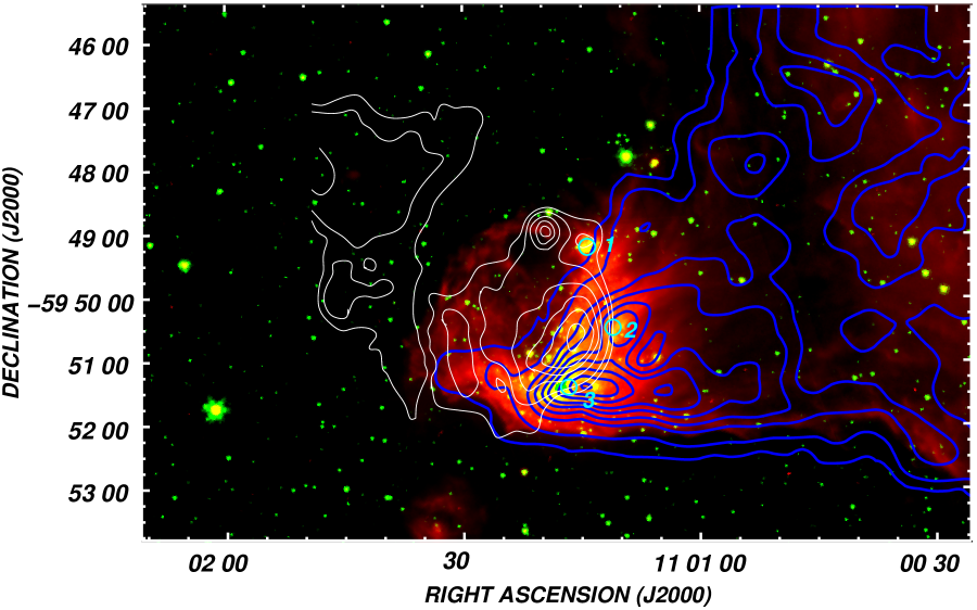
Figure 2: Composite image of NGC 3503 and its environs. Red and green show emission at 8.0 and 4.5 $\mu$m (IRAC-GLIMPSE), respectively. White and blue contours show the radio continuum 4800 MHz and integrated CO line emissions. Circles in light blue indicate the position of the three candidates to compact Hii  region identified in the MSX catalog (see Table 3 in Paper I). The CO temperature contours are 0.5 K km s^-1  ($\sim$10 rms), 1.5, 6.6, 10.5, 15.5, 20.5, 25.5, and 30.5 K km s^-1. The radio continuum 4800 MHz contours levels go from 2.4 mJy beam^-1 ($\sim$3 rms) to 10.4 mJy beam^-1 in steps of 2 mJy beam^-1, and from 10.4 mJy beam^-1in steps of 4 mJy beam^-1.

2.3 Physical parameters estimations

2.3.1 Excitation temperature and opacity

Excitation temperature ($T_{\rm exc}$) and opacity ($\tau$) of the CO(J=2$\rightarrow$1) and ¹³CO(J=2$\rightarrow$1) lines in Local Thermodynamic Equilibrium (LTE) conditions, can be derived using:

$$T_{\rm peak}=\ T_{0}\ [J(T_{\rm exc})\ -\ J(T_{\rm bg})]\ \times\ [1\ -\ e^{(-\tau)}]$$ (1)

(Dickman, 1978), where $T_{0}$ = $h\nu/k$, $J(T)=(e^{T_{0}/T}-1)^{-1}$, and $T_{\rm bg}$ is the background temperature (assumed to be $\sim$2.7 K). The excitation temperature of the ¹³CO(J=2$\rightarrow$1) line can be derived adopting $T_{\rm exc}$(¹³CO) $\approx$ $T_{\rm exc}$(CO), which can be calculated assuming that $\tau^{12}>>1$ and solving Eq. 1 as follows:

$$T_{\rm exc}{\rm(CO)}\ =\ \frac{T_{0}^{12}}{{\rm ln}\left[1\ +\ \frac{T_{0}^{12}}{T_{\rm peak}{\rm(CO)}\ +\ T_{0}^{12}\ \ [e^{(T_{0}^{12}/T_{\rm bg})}-1]^{-1}}\right]}\$$ (2)

where $T_{0}^{12}$ = $h\nu^{12}/k$, with $\nu^{12}$ = 230.538 GHz for the CO(J=2$\rightarrow$1) line. Then, the opacity of the ¹³CO(J=2$\rightarrow$1) line can be derived solving again Eq. 1:

$$\ \ \tau^{13}=-{\rm ln}\ [1\ -\ (T_{\rm mb}^{13}/T_{0}^{13})\ [(e^{T_{0}^{13}/T_{\rm exc}}\ -\ 1)^{-1}-\ (e^{(T_{0}^{13}/T_{\rm bg})}-1)^{-1}]^{-1}],$$ (3)

where $T_{0}^{13}$ = $h\nu^{13}/k$, with $\nu^{13}$ = 220.399 GHz. We can also estimate the optical depth of the CO(J=2$\rightarrow$1) line from the ¹³CO(J=2$\rightarrow$1) line with

$$\quad\tau^{12}=\ \left[\frac{\nu^{13}}{\nu^{12}}\right]^{2}\ \left[\frac{\Delta{\rm v}^{13}}{\Delta{\rm v}^{12}}\right]\ \left[\frac{\rm CO}{{}^{13}{\rm CO}}\right]\ \tau^{13},$$ (4)

where CO/¹³CO is the isotope ratio (assumed to be $\sim$ 62; Langer & Penzias 1993). $\Delta{\rm v}^{13}$ and $\Delta{\rm v}^{12}$ are defined as the full width half maximum (FWHM) of the spectrum of the ¹³CO and CO lines, respectively, which are derived by using a single Gaussian fitting (FWHM = 2 $\times$ $\sqrt{2\ ln2}$ $\times$ $\sigma_{\rm gauss}$).

2.3.2 Column density and mass

Assuming LTE conditions the H₂ column density, $N$(H₂), can be estimated from the ¹³CO(J=2$\rightarrow$1) line following the equations of Rohlfs & Wilson (2004)

$$N(^{13}{\rm CO})=1.5\times 10^{14}\ \ \frac{e^{[T_{0}(\nu_{10})/T_{\rm exc}]}\ \ T_{\rm exc}\int\tau^{13}\ \ d{\rm v}}{1-e^{[-T_{0}^{13}/T_{\rm exc}]}}\quad\textrm{ (cm${}^{-2}$)}$$ (5)

where $T_{0}(\nu_{10})$ = $h\nu_{10}/k$, being $\nu_{10}$ the frequency of the ¹³CO (1$\rightarrow$0) line (110.201 GHz). To solve the integral of Eq. 5 it can be assumed (in the limit of optically thin line) that $T_{\rm exc}\ \tau^{13}$ $\approx$ $T_{\rm mb}$. In any case, optical depth effects can be diminished using the approximation

$$T_{\rm exc}\ \int{\tau^{13}}d{\rm v}\approx\ \ [\tau^{13}/1-e^{(-\tau^{13})}]\ \int{T_{\rm mb}}\ \ d{\rm v}$$ (6)

This formula is accurate to 15 $\%$ for $\tau^{13}<2$. We also estimate an uncertainty of $\sim$ 20 $\%$ from determining $\int{T_{\rm mb}}$ $d$v. The molecular mass is then calculated using

$$M(\rm H_{2})\ =\ {\it m}_{\rm sun}^{-1}\ \ \mu\ \ {\it m}_{H}\ \ \sum\ \ \Omega\ \ {\it N}(\rm H_{2})\ \ {\it d}^{2}\quad\quad\quad\textrm{(M${}_{\odot}$)}$$ (7)

where $m_{\rm sun}$ is the solar mass ($\sim$ 2 $\times$ 10³³ g), $\mu$ is the mean molecular weight, which is assumed to be equal to 2.72 after allowance of a relative helium abundance of 25% by mass (Allen, 1973), $m_{\rm H}$ is the hydrogen atom mass ($\sim$ 1.67 $\times$ 10^-24 g), $\Omega$ is the solid angle subtended by the CO feature in ster, $d$ is the distance (assumed to be 2.9 $\pm$ 0.4 kpc; see Paper I) expressed in cm, and $N$(H₂) is obtained using a “canonical” abundance $N(\rm H_{2})$ / $N(^{13}{\rm CO})$ = 5 $\times$ 10⁵ (Dickman, 1978).

Considering only gravitational and internal pressure, neglecting support of magnetic fields or internal heating sources, and assuming a spherically symmetric cloud with a $r^{-2}$ density distribution, the virialized molecular mass, $M_{\rm vir}$, can be estimated from

$$\quad M_{\rm vir}\ =\ 126\ R_{\rm eff}\ (\Delta{\rm v}_{\rm cld})^{2}\qquad\qquad\textrm{(M${}_{\odot}$)}$$ (8)

(MacLaren et al., 1988), where $R_{\rm eff}$ = $\sqrt{A_{\rm cloud}/\pi}$ is the effective radius in parsecs, and $\Delta{\rm v}_{\rm cld}$ is the width of the composite spectrum, defined as for $\Delta{\rm v}^{13}$ and $\Delta{\rm v}^{12}$ in Eq. 4. The composite spectrum is obtained by averaging all the spectra within the area of the cloud ($A_{\rm cloud}$).

The mass of the dust can be calculated following Deharveng et al. (2009). Considering that the emission detected at 870 $\mu$m originates in thermal dust emission, the dust mass ($M_{\rm dust}$) can be derived from

$$\quad M_{\rm dust}\ =\ \frac{S_{870}\ d^{2}}{\kappa_{870}\ J_{870}(T_{\rm dust})},$$ (9)

where $S_{870}$ is the measured flux density, $d$ is the adopted distance to the source, $\kappa_{870}$ is the dust opacity per unit mass at 870 $\mu$m , and $J_{870}(T_{\rm dust})$ is the Planck function for a temperature $T_{\rm dust}$. We adopted a dust opacity $\kappa_{870}$ = 1.0 cm² g^-1 estimated for dust grains with thin ice mantles in cold clumps (Ossenkopf & Henning, 1994).

3 Results and analysis of the observations

3.1 Spatial distribution of the molecular gas

To study the molecular gas associated with NGC 3503  we have mostly focused on Component 1 of Paper I (which is undoubtedly associated with the nebula). We will also make a brief analysis of the molecular gas associated with Component 2 and Component 3.

In Fig. 2 we show an overlay of the mean CO emission as obtained with APEX, in the velocity interval from $-$29 km s^-1 to $-$24 km s^-1, onto the IRAC-GLIMPSE (Benjamin et al., 2003) and 4800 MHz radio continuum emission of the nebula. Though a remarkable resemblance between CO and IR emission (MSX-A band) was previously put forward in Paper I, specially towards the extended IR emission at north and east of NGC 3503 (see Fig. 6 of that work), a tight morphological correlation between the IR nebula and the molecular gas in the studied velocity interval is revealed by our new APEX observations, which confirms that this cloud is physically associated with the IR nebula. From Fig. 2, a direct comparison of the molecular and 4800 MHz radio continuum emissions strongly suggests that the molecular gas is being compressed by an ionization front and is interacting with the nebula. On the other hand, the ionized gas seems to be expanding freely towards the opposite direction (i.e. the intercloud medium). The location of the PDR is traced by the emission of PAHs molecules in the 8.0 $\mu$m image (red colour). Since these complex molecules are destroyed inside the ionized gas of an Hii  region (see Deharveng et al. 2010 and references therein), they delineate the boundaries of NGC 3503. The molecular gas clearly depicts the position of the ionization front. As predicted in Paper I, no molecular emission is detected in this velocity range towards the low electron density region, which is compatible with a champagne-flow scenario. However, we speculate that the IR arc-like filament (from here onwards the “IR arc”) seen in the northeastern border of the nebula at RA, Dec. (J2000) $\sim$ (11^h01^m30^s, $-$59^∘50′10″) and RA, Dec. (J2000) $\sim$ (11^h01^m25^s, $-$59^∘49′00″), might be still associated with small amounts of molecular gas at velocities between $\sim$ $-$17.1 to $-$15.3 km s^-1 (see Sect. 3.2).

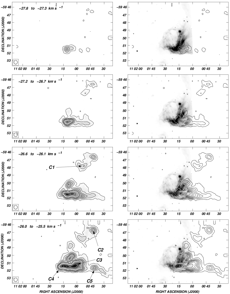
Figure 3: Left panels: Integrated ¹³CO emission in the velocity range from $\sim$ $-$27.8 to $-$23.7 km s^-1, and from 18.7 to 21.7 km s^-1 (see continuation). The velocity interval of each image is indicated in the upper left corner. The lowest temperature contour is 0.7 K km s^-1($\sim$ 5 rms). The contour spacing temperature is 1.5 K km s^-1 to 9.7 K km s^-1, and 4 K km s^-1 hereonwards. The beam size is shown by a circle in the lower left corner of each image. Right panels: Overlay of the IRAC GLIMPSE 4 (8 $\mu$m) emission of NGC 3503 (grayscale) and the mean ¹³CO emission in the velocity intervals shown in the left panels (contour lines).

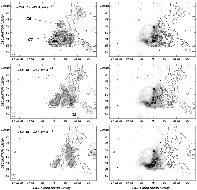
Figure 3: continuation

Figure 4: Left panels: Integrated ¹³CO emission in the velocity range from $\sim$ $-$17.1 to $-$15.3 km s^-1(upper panel), and from 18.7 to 21.7 km s^-1 (lower panel). The velocity interval of each image is indicated in the upper left corner. In the upper panel, the lowest ¹³CO temperature contour is 0.35 K km s^-1($\sim$ 5 rms) and the contour spacing temperature is 0.7 K km s^-1. In the lower panels, the lowest ¹³CO temperature contour is 0.75 K km s^-1 ($\sim$ 15 rms) and contour spacing temperature is 1 K km s^-1. The beam size is shown by a circle in the lower left corner of each image. Right panels: Overlay of the IRAC GLIMPSE 4 (8 $\mu$m) emission of NGC 3503 (grayscale) and the mean ¹³CO emission in the velocity intervals shown in the left panels (contour lines).

Since the CO(J=2$\rightarrow$1) line is optically thick and can be used only to trace low density gas, we analyze the ¹³CO data which allows one to go deeper into the molecular clouds, although it may fail to probe the densest molecular gas because it freezes onto dust grains at high densities (Massi et al., 2007). To study the kinematics of the molecular gas in more detail we have averaged the individual original channel maps of the ¹³CO emission line. In Fig. 3 (left panels) we show a collection of narrow velocity images depicting the mean ¹³CO spatial distribution in the velocity range from $-$27.8 km s^-1  to $-$23.7 km s^-1. Every image represents an integral of the ¹³CO emission $\int$ $T_{\rm mb}\ d{\rm v}$ (K km s^-1) over a velocity interval of 0.5 km s^-1. In this way, the final rms noise for each interval results $\Delta T_{\rm rms}$ $\approx$ 0.15 K km s^-1. To analyze the relation between the molecular gas and the warm dust in the nebula, in the right panels of Fig. 3 we show the ¹³CO emission in the velocity intervals mentioned before (in contours) projected onto the IRAC GLIMPSE-4 (8 $\mu$m) emission of NGC 3503 (grayscale). In order to study the small-scale structure of the molecular cloud we have identified a number of small molecular clumps. The clumps were selected by eye and based in the following simplest criteria: 1) the peak temperature of each clump is at least 5 times the rms noise, 2) the decrease in $T_{\rm mb}$ between the peak temperature of two adjacent clumps is larger than 5 times the rms noise, and 3) the clump is present at least along $\sim$40 $\%$ of the total velocity interval of the cloud. We define the area of each clump ($A_{\rm clump}$) by the polygon that encloses the emission corresponding to half the $T_{\rm mb}$ peak in the velocity interval at which the clump is observed. The clumps are indicated in Fig. 3 from C1 to C8 and the labeling was made in the velocity interval at which they reach the maximum emission peak temperature. Such molecular clumps are also identified in CO showing more extended emission.

The molecular emission becomes first noticeable in the velocity interval from $-$27.8 km s^-1  to $-$27.3 km s^-1  as a weak patchy structure centered at (RA, Dec. (J2000)) $\simeq$ (11^h01^m10^s, $-$59^∘51′30″). Within the velocity range from $-$27.2 km s^-1to $-$26.7 km s^-1  most of the emission comes from a broad and cometary head-tailed structure lying along Dec.(J2000) $\approx$ $-$59^∘51′30″ that is coincident with the optical feature SFO 62 (see Fig. 1). This coincidence might confirm that this molecular feature is being ionized from a stellar source/s at lower declinations giving rise to the BRC, as previously suggested in Paper I. This structure shows a sharp cut-off in the direction of NGC 3503  which suggests an interaction between the Hii  region and the molecular gas. Very likely, the molecular gas has undergone compression on the front side due to the expansion of the ionized gas and/or the stellar winds of members of Pis 17. This trend is also observed in the CO emission. Between $-$26.6 km s^-1  to $-$26.1 km s^-1  a molecular emission maximum, detected close to the brightest IR region of NGC 3503  at (RA, Dec. (J2000)) $\approx$ (11^h01^m15^s, $-$59^∘51′25″), appears to be merged with the lengthened molecular structure along Dec(J2000) $\approx$ $-$59^∘51′30″. A molecular clump, C1, is indicated in this velocity interval, located at (RA, Dec. (J2000)) $\approx$ (11^h00^m50^s, $-$59^∘47′57″). This clump is detected in the total velocity range from $-$27.1 to $-$25.6 km s^-1.

In the velocity range from $-$26.0 km s^-1  to $-$25.5 km s^-1 the molecular emission shows a good morphological resemblance with the IR nebula. Four molecular clumps achieve the maximum emission temperature at this velocity range. Clump C2 is placed adjacent to C1, at (RA, Dec. (J2000)) $\approx$ (11^h00^m40^s, $-$59^∘46′40″) and is identifiable in the total velocity range from $-$27.3 to $-$24.3 km s^-1. A moderately intense extended emission seems to be connecting both clumps, which may indicate a physical association. Clumps C3 and C4 are located at (RA, Dec. (J2000)) $\approx$ (11^h01^m05^s, $-$59^∘51′30″) and (RA, Dec. (J2000)) $\approx$ (11^h01^m12^s, $-$59^∘51′25″), respectively. Their locations are coincident with the cometary head-tailed feature observed between $-$27.2 km s^-1to $-$26.7 km s^-1which means that they all are part of the same molecular structure. This correlation suggests that the formation of clumps C3 and C4 are the result of a fragmentation due to the compression of the Hii  region (Whitworth et al., 1994), although previous estimates seem to discredit this conjecture (see Paper I). The molecular emission in the direction of these clumps is detected almost in the entire velocity range. The position of C4 is highly coincident with an MSX compact Hii  region candidate labeled as source 3 in Paper I (see Fig. 2).

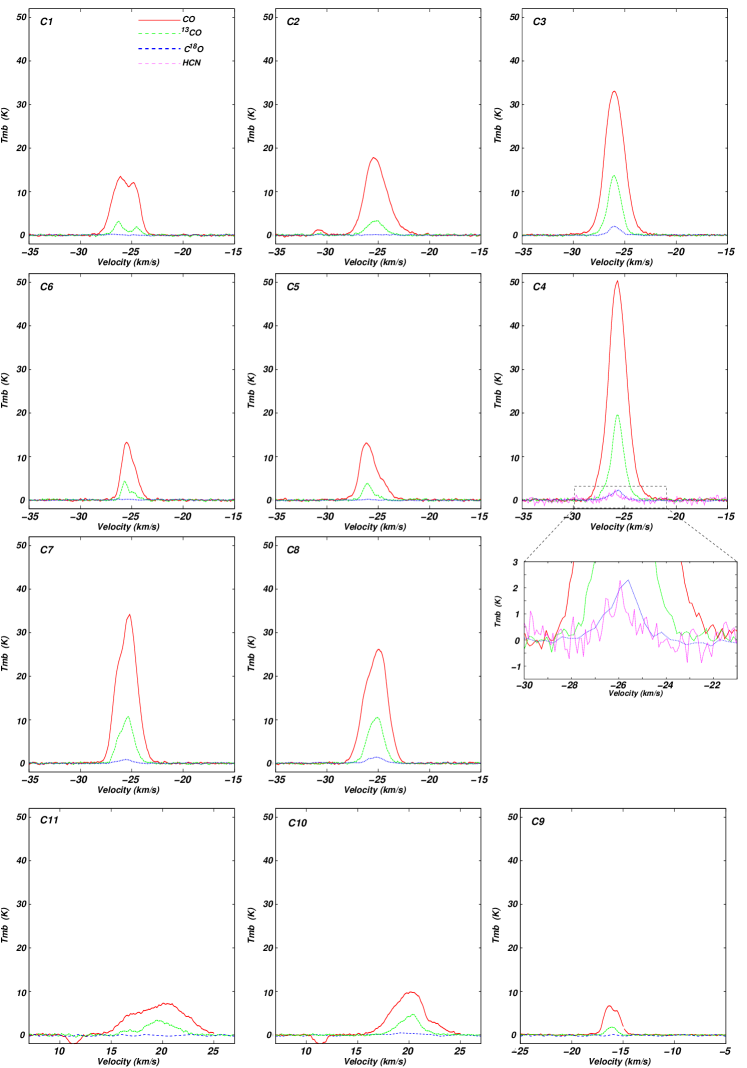
Figure 5: CO, ¹³CO, and C¹⁸O averaged line spectra obtained towards the molecular clumps C1 to C11. For C4, the spectrum of HCN is zoomed in the middle right panel of the figure.

This suggests that C4 is a high density molecular clump that is been irradiated by the UV field of NGC 3503. The fourth molecular clump detected in this velocity range, C5, is located at (RA, Dec. (J2000)) $\approx$ (11^h00^m40^s, $-$59^∘51′30″). Its location is almost adjacent with the westernmost border of SFO 62   (see Fig. 1) and its eastern border seems to be connected with the western side of C3 by a weak bridge of ¹³CO emission. The molecular emission of C5 is detectable up to $-$24.9 km s^-1. C3, C4, and C5 are detected in the total velocity range from $-$27.1 to $-$24.9 km s^-1, $-$27.8 to $-$24.5 km s^-1, and $-$26.6 km s^-1 to $-$24.6 km s^-1, respectively. Probably, the leakage of UV radiation of SFO 62   into the molecular gas might have helped to shape clumps C3, C4, and C5 (e.g. Pomarès et al. 2009).

Table 2: Geometrical and line emission parameters obtained for the molecular clumps

Clump	RA	Dec.(J2000)	$A_{\rm clump}$(13CO)	$T^{13}_{\rm peak}$	$T^{18}_{\rm peak}$	$T^{12}_{\rm peak}$	$T^{\rm HCN}_{\rm peak}$	v${}^{13}_{\rm centr}$	Vel. int. (13CO)
	(h m s)	(∘ ′ ″)	(10-8 ster)	(K)	(K)	(K)	(K)	(km s-1)	(km s-1)
C1	11 : 00 : 52	$-$59 : 47 : 57	7.8	3.2	-	13.6	-	$-$26.3	$-$27.1 to $-$25.6
C2	11 : 00 : 40	$-$59 : 46 : 40	7.3	3.4	-	17.9	-	$-$25.3	$-$27.3 to $-$24.3
C3	11 : 01 : 05	$-$59 : 51 : 30	10.7	13.7	$\sim$ 2.1	33.2	-	$-$26.0	$-$27.1 to $-$24,9
C4	11 : 01 : 12	$-$59 : 51 : 25	8.6	19.7	$\sim$ 2.3	50.3	$\sim$ 2.3	$-$25.7	$-$27.8 to $-$24.5
C5	11 : 00 : 40	$-$59 : 51 : 30	5.5	3.8	-	13.3	-	$-$26.1	$-$26.6 to $-$24.6
C6	11 : 01 : 06	$-$59 : 48 : 40	4.1	4.3	-	13.4	-	$-$25.7	$-$26.1 to $-$25.0
C7	11 : 01 : 10	$-$59 : 50 : 28	8.9	10.7	$\sim$ 0.9	34.2	-	$-$25.5	$-$27.1 to $-$24.7
C8	11 : 00 : 53	$-$59 : 51 : 00	8.6	10.5	$\sim$ 1.5	26.2	-	$-$25.2	$-$25.6 to $-$24.1
C9	11 : 01 : 37	$-$59 : 50 : 00	9.1	1.8	-	6.7	-	$-$16.1	$-$17.1 to $-$15.3
C10	11 : 01 : 11	$-$59 : 48 : 57	3.9	4.7	-	9.9	-	20.1	17.2 to 22.5
C11	11 : 01 : 05	$-$59 : 47 : 40	6.0	3.3	-	7.3	-	20.9	15.3 to 22.8

Table 3: Physical and dynamical properties derived for the molecular clumps.

Clump	$T_{\rm exc}$	$\tau^{13}$	$\tau^{12}$	$\Delta{\rm v}^{\rm 13}$	$\Delta{\rm v}^{12}$	$\frac{\Delta{\rm v}^{\rm 13}}{\Delta{\rm v}_{\rm th}^{\rm 13}}$	$N(\rm H_{2})^{\rm peak}_{\rm LTE}$	$N(\rm H_{2})^{\rm level}_{\rm LTE}$	$M_{\rm LTE}$	$M_{\rm vir}$	$\frac{M_{\rm LTE}}{M_{\rm vir}}$
	(K)			(km s-1)	(km s-1)		(1021 cm-2)	(1021 cm-2)	(M⊙ )	(M⊙ )
C1	18.7	0.26	7.1	0.91	1.92	5.4	1.2 $\pm$ 0.2	0.8 $\pm$ 0.2	11 $\pm$ 5	36 $\pm$ 12	$\sim$ 0.3
C2	23.1	0.21	9.0	1.82	2.41	9.6	3.3 $\pm$ 0.7	2.2 $\pm$ 0.4	29 $\pm$ 15	170 $\pm$ 55	$\sim$ 0.2
C3	39.1	0.51	19.6	1.48	2.20	5.9	13.8 $\pm$ 2.7	9.8 $\pm$ 1.9	191 $\pm$ 95	147 $\pm$ 50	$\sim$ 1.3
C4	57.2	0.48	17.6	1.39	2.13	4.5	27.1 $\pm$ 5.4	18.2 $\pm$ 3.6	282 $\pm$ 140	120 $\pm$ 41	$\sim$ 2.4
C5	18.3	0.33	12.7	1.03	1.53	6.1	1.6 $\pm$ 0.3	1.2 $\pm$ 0.2	12 $\pm$ 6	51 $\pm$ 17	$\sim$ 0.2
C6	18.5	0.38	13.1	0.77	1.25	4.5	1.3 $\pm$ 0.3	0.9 $\pm$ 0.2	7 $\pm$ 3	22 $\pm$ 8	$\sim$ 0.3
C7	39.7	0.37	14.2	1.53	2.26	6.1	10.0 $\pm$ 2.1	6.5 $\pm$ 1.3	169 $\pm$ 84	144 $\pm$ 49	$\sim$ 1.2
C8	31.6	0.50	19.0	1.61	2.42	8.1	8.5 $\pm$ 1.7	5.8 $\pm$ 1.2	92 $\pm$ 46	165 $\pm$ 56	$\sim$ 0.6
C9	11.5	0.29	10.3	1.15	1.81	8.3	1.4 $\pm$ 0.3	0.4 $\pm$ 0.1	6 $\pm$ 3	79 $\pm$ 28	$\sim$ 0.1
C10	15.2	0.62	18.5	1.92	3.62	12.4	8.0 $\pm$ 1.6	5.6 $\pm$ 1.1	303 $\pm$ 90(†)	408 $\pm$ 83(†)	$\sim$ 0.7
C11	12.2	0.58	24.2	3.11	4.23	22.2	7.1 $\pm$ 1.4	4.9 $\pm$ 1.0	408 $\pm$ 82(†)	1340 $\pm$ 270(†)	$\sim$ 0.3

Notes: $({\dagger})$ Values obtained adopting a kinematical distance of 8 kpc. Uncertainties were calculated taking into account only innacuracies in the boundary selection.

In the velocity range from $-$25.4 to $-$24.9 km s^-1 clumps C6 and C7 achieve their maximum emission temperature. Clump C6, located at (RA, Dec. (J2000)) $\approx$ (11^h01^m07^s, $-$59^∘48′40″), is observed in a small velocity interval ($-$26.1 to $-$25.0 km s^-1) and is not morphologically correlated with the nebula. On the other hand, clump C7, placed at (RA, Dec. (J2000)) $\approx$ (11^h01^m10^s, $-$59^∘50′30″), is projected onto the IR nebula and close to the location of the MSX compact Hii region candidate labeled as source 2 in Paper I (see Fig. 2). Clump C7 is detected over a velocity interval from $-$27.1 to $-$24.7 km s^-1.

In the velocity interval from $-$25.4 to $-$24.9 km s^-1clump C8 becomes noticeable as a patchy structure at (RA, Dec. (J2000)) $\approx$ (11^h00^m52^s, $-$59^∘51′00″), merged to clump C3. It achieves its maximum emission temperature in the velocity range from $-$24.8 to $-$24.3 km s^-1. It is barely detected beyond a velocity of $\sim$ $-$23.7 km s^-1. Clump C8 is almost adjacent to SFO 62 which indicates that this clump might be affected by the BRC.

It is worth mentioning that the C¹⁸O(J=2$\rightarrow$1) line emission, which is a good tracer of high density molecular gas, is only detected in the velocity range from $\sim$ $-$26.5 to $-$25.1 km s^-1, and is mostly concentrated towards the position of clumps C3, C4, and C7 (see Sect. 3.6)

In Fig. 4 (upper panels) we show the ¹³CO emission distribution integrated in the velocity interval from $-$17.1 to $-$15.3 km s^-1. A relatively extended patchy structure is observed at (RA, Dec. (J2000)) $\simeq$ (11^h01^m37^s, $-$59^∘50′00″). For the sake of the convention, this structure is identified as clump C9. This molecular clump was reported in Paper I as Component 2. From a comparison with the IR emission (right panel) it can be noticed a good correspondence between the external border of C9 with the IR arc which suggests a physical association between this clump and the nebula.

From a spectrum obtained in the direction of the MSX CHii region candidate source 1 (from Paper I) we can observe that the bulk of the molecular emission is in the velocity range from $\sim$ 19 to 22 km s^-1. In Fig. 4 (lower panels) we show the molecular emission integrated in the velocity range from 18.7 to 21.7 km s^-1. From this figure, it can be noted a molecular structure (from here onwards clump C10) almost projected over source 1. The circular galactic rotation model by Brand & Blitz (1993) locates this clump at 8 kpc. Probably, it is associated with the larger molecular structure reported in Paper I as Component 3. In the same velocity range another molecular structure (clump C11) is observed at (RA, Dec. (J2000)) $\approx$ (11^h01^m05^s, $-$59^∘47′40″), which is probably associated with clump C10. Since the radio continuum image at 4800 MHz indicates the presence of ionized gas in the direction of C10, further radio recombination line observations may help to confirm or discard the velocity interval and a physical association between this molecular clump and source 1. Nevertheless, the disparity in the central velocities between C10 and C11 with the rest of the clumps ($\sim$45 km s^-1) suggests that these clumps are physically unrelated to NGC 3503. Assuming a distance of $\sim$ 8 kpc, clumps C10 and C11 turn out to be the most massive clumps in the sample (see Table 3, Sect 3.2).

In Fig. 5 we show the averaged CO(J=2$\rightarrow$1), ¹³CO(J=2$\rightarrow$1), and C¹⁸O(J=2$\rightarrow$1) spectra obtained inside the emission temperature level which defines each $A_{\rm clump}$. In Table 2 we present some morphological properties of the clumps and averaged emission line parameters obtained in their direction. Columns (2) and (3) give the coordinates of the center of the clumps. Column (4) lists the area of each clump. In columns (5), (6), (7), and (8) the peak emission of the ¹³CO, C¹⁸O, CO, and HCN lines are given. The C¹⁸O and HCN peak temperatures are listed only when a value at least 3 rms noise is achieved. In column (9) we list the central velocity obtained by gaussian fitting of the integrated ¹³CO spectra within $A_{\rm clump}$, and column (10) indicates the velocity interval of the ¹³CO line at which each clump is detected.

3.2 Physical properties of the molecular gas

In the previous section we analyzed the morphological and kinematical properties of the molecular gas in the velocity interval from $\sim$ $-$28 to $-$24 km s^-1, $-$17.1 to $-$15.3 km s^-1, and 18.7 to 21.7 km s^-1  in the environs of NGC 3503 and SFO 62 . Morphological characteristics clearly evidence a physical association between the Hii  region and the BRC with the molecular clumps identified within the velocity interval from $\sim$ $-$28 to $-$24 km s^-1, and probably from $-$17.1 to $-$15.3 km s^-1. In this section, we analyze and compare the physical properties of the molecular clumps aimed at finding some influence of shock fronts or UV radiation on the molecular gas. We include a brief comment on C10 and C11 although, as mentioned before, a physical association of these clumps with NGC 3503 is doubtful.

In Table 3 we list some important physical and dynamical properties derived for the molecular clumps using the averaged spectra from Fig. 5. Column (2) lists the excitation temperature obtained from the CO peak and using Eq. 2. Columns (3) and (4) give the optical depth of ¹³CO and CO, obtained with Eqs. 3 and 4, respectively. The width of ¹³CO and CO lines ($\Delta{\rm v}^{\rm 13}$ and $\Delta{\rm v}^{\rm 12}$), defined as the FWHM of the line (see Sect. 2.3.1), is tabulated in columns (5) and (6), respectively. The ratio between $\Delta{\rm v}^{\rm 13}$ and the expected thermal width is listed in column (7). The expected thermal width of ¹³CO is estimated using $\Delta{\rm v}_{\rm th}^{\rm 13}=\sqrt{8\ ln2\ k\ T_{\rm k}/m}$, where $k$ is the Boltzman constant, $T_{\rm k}$ is the kinetic temperature (assumed to be equal to $T_{\rm exc}$), and $m$ is the mass of the ¹³CO molecule. The line widths of the CO and ¹³CO spectra were derived from Gaussian fittings averaging all the spectra within $A_{\rm clump}$. Columns (8) and (9) give the column densities at the emission peak and averaged within $A_{\rm clump}$, respectively. The mass derived assuming LTE and virial equilibrium is listed in columns (10) and (11), respectively. There are some uncertainties in measuring $M_{\rm LTE}$ and $M_{\rm vir}$. In both cases, the values are affected by a distance indetermination of $\sim$ 15 $\%$ ($d$ = 2.9 $\pm$ 0.4 kpc) which yields to uncertainties of $\sim$ 30 $\%$ for $M_{\rm LTE}$ ($M_{\rm LTE}$ $\propto$ $d^{2}$) and $\sim$ 15 $\%$ for $M_{\rm vir}$ ($M_{\rm vir}$ $\propto$ $d$). In addition, inaccuracies in the boundary selection ($\sim$ 20 $\%$) can affect the size estimation of the clumps and therefore to produce significant uncertainties in the mass calculations, since a considerable part of the molecular mass could be missed, especially for the cases of clumps C3, C4, C7 and C8 (they have very high emission temperature boundaries above the minimum 5 rms noise). We estimate total uncertainties of about $\sim$ 50 $\%$ and $\sim$ 30 $\%$ for $M_{\rm LTE}$ and $M_{\rm vir}$, respectively. It is also worth mentioning that when abundances and isotopologic ratios are considered, accuracy might be within a factor of 2. From Table 3, it can be noted that $\Delta{\rm v}^{12}$ is, in average, larger than $\Delta{\rm v}^{13}$ by a factor of 1.5. Since the CO molecule is optically thick, some asymmetries in its spectra might be misjudged. For example, clump C1 exhibits a double peak profile in its CO spectrum. This could be a result of self-absorption, which could indicate the existence of hot/warm gas inside the clump. While, the emission of ¹³CO clearly suggests the existence of a double cloud in the line of sight at different velocities (see Figs. 3 and 5). Then, having the two isotopes provides a tool to discern the numbers of components along the line of sight. Similarly, the CO spectra of C5 and C6 show small “shoulders”. An inspection at their ¹³CO spectra suggests that these shoulders are the result of a second weaker component at more positive velocities (see also Fig. 3). As a result, the virial masses using $\Delta{\rm v}^{12}$ might be overestimated. Then, we used $\Delta{\rm v}^{13}$ for the calculations. For C1, C5, and C6 we take into account only the strongest molecular components (at more negative velocities).

Molecular clumps that are close to the ionized gas are expected to have different properties than those distant from it, mostly due to shock fronts and stellar FUV radiation impinging onto the cloud. To search for their influence on the molecular gas we analyze the physical properties listed in Table 3.

An analysis of temperatures and densities would be very instructive in this matter. Since $T_{\rm exc}$ is derived using the optically thick CO(J=2$\rightarrow$1) emission, it probes the surface conditions of the clouds. An inspection at Table 3 shows that clumps C1, C2, C5, and C6 (from here onwards the “cold clumps”) achieve temperatures in a range between $\sim$ 18 - 23 K. These values are typical in cold molecular clouds, where cosmic ray ionization is the main heating source. Clumps C3, C4 and C7 (from here onwards the “warm clumps”) achieve temperatures in the range $\sim$ 39 - 57 K which suggests that additional local heating sources are present. Clumps C4 and C7 lie at the edge of NGC 3503 and they appear to have been externally heated through the photoionization of their surface layers, as proposed in Paper I. This is reinforced by the presence of a PDR at the interface between the nebula and the clumps (see Fig. 2). For the case of C3, its location (adjacent to SFO 62 , see Figs. 1 and 2) would explain its high temperature (39.1 K). It is also worth to mention that the warm clumps have also higher column densities, which very likely indicates that they are actually formed by gas that has been swept up by the expansion of the ionization and has been condensed. An inspection at Figs. 1 and 2 shows that C4 is “trapped” between two ionization fronts (NGC 3503 and SFO 62 ). Then, there might be additional compression, heating and ionization acting upon C4, which might explain the high surface temperature and density derived for this clump. Furthermore, it is the only clump detected in HCN emission (see Sect. 3.4). We keep in mind, however, that Pis 17 has probably been formed inside high density molecular gas nearby to C4 and C7 that was later evacuated, so an increment in the density of the molecular environment is expected. In addition, star forming process that are likely occurring inside clumps C3, C4 and probably C7 (see Sect. 3.6) may be contributing in rising the temperature. Temperature and density of C8 are above than those of cold clumps, which might implicate external sources of heating and compression. Although this clump appears to be more distant of SFO 62  than C3, an interaction with the ionized gas of the BRC cannot be discarded.

It is also expected that clumps neighboring the Hii  region exhibit signs of turbulence which could be manifested as line widths significantly broadened. However, an inspection of Table 3 shows that all the clumps exhibit line broadenings beyond the natural thermal width. Different from expected, the molecular emission towards clump C2 (which is the most distant to an ionization front), shows the broadest averaged spectra, while clump C4, which clearly shows signs of interactions with the ionization fronts of NGC 3503 and SFO 62 (see the above paragraph), exhibits the lowest ratio between observed and thermal widths. Probably, the line width of the averaged spectrum reflects that different parts of the clouds inside $A_{\rm clump}$ have different velocities, rather than showing turbulence effects. Further, the angular resolution of the observations may not suffice to resolve objects and/or effects in the molecular gas (e.g. outflows, infall, accretion, etc.) that may be contributing in the broadening of the emission line.

Warm clumps have the highest LTE masses (71 to 282 M_⊙ ), in comparison with colder clumps (7 to 29 $M_{\odot}$). This trend is also observed with virialized masses with the exception of C2. An inspection at Table 3 shows that for the case of cold clumps the ratio $M_{\rm LTE}/M_{\rm vir}$ is in the range 0.2 to 0.3. On the other hand, for the case of warm clumps mass ratios $M_{\rm LTE}$/$M_{\rm vir}$ $>$ 0.6 were obtained (predominantly $>$1). Special attention may require for the case of clump C4, since its $M_{\rm LTE}$ is more than twice larger than $M_{\rm vir}$. Classical Virial equilibrium analysis establishes that the virial mass is the minimum mass required in order for a cloud to be gravitationally bound. Then, if $M_{\rm vir}$ is larger than $M_{\rm LTE}$ the cloud has too much kinetic energy and is unstable. That seems be the case for cold clumps which are probably expanding as a result of a lack of an external stabilizing pressure. Differently, warm clumps seem to be in virial equilibrium (gravitationally bound) which suggests that the ionization front and UV radiation of the Hii  region is sufficient to heat up, but not enough to disrupt the molecular gas of the clump. The presence of two protostellar candidates projected onto the direction of C4 (see Sect. 3.6) might indicate that infalling motions may be occurring inside this clump, which is in line with its high $M_{\rm LTE}$/$M_{\rm vir}$ ratio. Nevertheless, new observational results suggest that physical properties of molecular clouds do not agree with the classical interpretation of virial equilibrium (balance between gravitational and kinetic energies) in the sense that an external pressure acting like confining force is needed (Heyer et al., 2009; Field et al., 2011). We also keep in mind the caveats in the line width determination (see previous paragraph), and hence in determining $M_{\rm vir}$, which could lead us to mistakenly interpret the results. Higher spatial resolution observations might help to achieve more conclusive results.

We have excluded clumps C9, C10, and C11 from the previous analysis, since it is not clear whether they are physically associated with NGC 3503. As mentioned in Sect. 3.1, the external border of C9 shows a good correspondence with the IR arc. The low density and mass derived for C9 (see Table 3) suggests that this feature might be some residuary molecular gas from the original parental cloud after the Hii  region have blown into the intercloud medium. The location of C9 (in the opposite side of clumps C4 and C7) and its velocity (shifted by $\sim$ 10 km s^-1) is in line with this scenario. Clumps C10 and C11 display the largest line widths (and low excitation temperatures), with complex spectra typical of the presence of several velocity components. These characteristics add more support to our previous assumption that clumps C10 and C11 are physically unrelated to the rest of the molecular gas associated with the nebula.

3.3 The velocity field of C4

In the previous section, we analyzed the line width of the averaged clump spectra to look for signposts of a kinematical disturbance produced by the Hii  region. Different from expected, the averaged spectrum of clump C4 does not seem to be significantly broadened (when compared with the rest of the clumps) by the action of the Hii  region. However, a careful inspection at Fig. 3 shows that the spatial location of the peak emission of C4 is slightly displaced from RA. = 11^h01^m14^s to RA. = 11^h01^m16^s in the velocity range from $-$27.8 to $-$24.9 km s^-1, which gives rise to a small velocity gradient. In Fig.6 we show the position-velocity map along Dec.(J2000) = $-$59^∘51′20″, slicing clumps C3, C4, and C5. Unlike C3 and C5, a noticeable velocity gradient in the peak emission of C4 is detected around the central position of the IR nebula. This velocity gradient can be directly connected to the nebula and could be interpreted as a significant sign of the disturbance in the molecular gas next to the ionization front. According to this interpretation, the expansion of the ionized gas might be affecting the kinematics of the molecular gas adjacent to it (clump C4) giving rise to this kinematical feature. An alternative explanation might be provided from the analysis of the 870 $\mu$m emission (see Sect. 3.5). In Figs. 10 and 12 two molecular cores (identified in Sect. 3.5 as D1 and D2) can be noticed in the 870 $\mu$m emission (HPBW = 19^′′) inside the ¹³CO(J=2$\rightarrow$1) and C¹⁸O(J=2$\rightarrow$1) emission of clump C4. Probably, C4 is composed by two different molecular cores at slightly different velocities which are not resolved by carbon monoxide observations (HPBW = 27^′′ - 28^′′). These cores can be also noticed in the HCN(J=3$\rightarrow$2) emission (see Figs. 7 and 12).

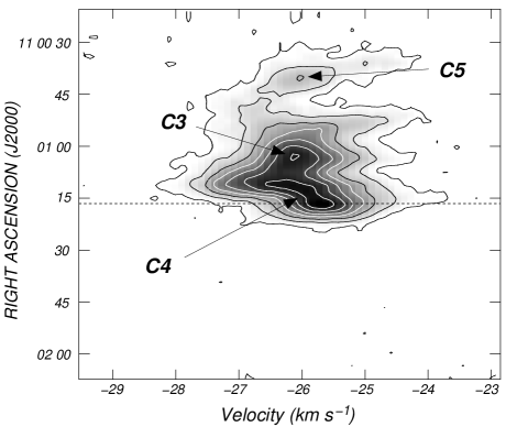
Figure 6: ¹³CO position-velocity map along Dec.(J2000) = $-$59^∘51′20″. The position of the center of NGC 3503 is indicated by the dotted line.

3.4 Denser gas: LVG modeling

In Fig. 5 we have shown that clump C4 has the only detection in the HCN line, at a velocity of $\sim$ $-$26 km s^-1. In Fig. 7 we show an overlay of the mean HCN emission in the velocity interval from $-$26.5 km s^-1to $-$25.5 km s^-1 onto the IRAC-GLIMPSE 4 emission of the nebula.

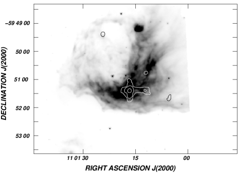
Figure 7: Mean HCN emission in the velocity range from $-26.5$ to $-25.5$ km s^-1(contours) superimposed onto the IRAC-4 image of the nebula (grays). The lowest temperature contour is 0.55 K km s^-1 ($\sim$5 rms) and contour spacing temperature is 0.33 K km s^-1.

The image shows four small sources placed at RA, Dec. (J2000) = (11^h01^m05^s, $-$59^∘51′40″), RA, Dec. (J2000) = (11^h01^m25^s, $-$59^∘49′22″), RA, Dec. (J2000) = (11^h01^m12^s, $-$59^∘50′40.5″), and RA, Dec. (J2000) = (11^h01^m14.6^s, $-$59^∘51′22.7″). The first three sources are observed in their detection limits ($\sim$ 5 rms) and will not be considered to further analysis. The fourth source is more extended and achieves a peak temperature of $\sim$2 K at RA, Dec. (J2000) = (11^h01^m16.7^s, $-$59^∘51′23″).

Figure 8: LVG models for ¹³CO and HCN peak temperatures as function of normalized column density and volume density. We adopted abundances [¹³CO]/[H₂] = 2 $\times$ 10^-6 and [HCN]/[H₂] = (2 - 20) $\times$ 10^-8. The green lines trace the contours of ¹³CO peak intensity, while the red lines trace the contours of HCN peak intensity. Dotted black lines are where solutions are coincident.

A second and weaker peak temperature ($\sim$ 0.8 K) is observed at RA, Dec. (J2000) = (11^h01^m11.6^s, $-$59^∘51′23.1″). The spatial location of this source is coincident with the ¹³CO emission of C4, which clearly suggests that its emission represents the HCN counterpart of that molecular clump. The position of the two emission peaks in the HCN line at RA, Dec. (J2000) = (11^h01^m16.7^s, $-$59^∘51′23″) and RA, Dec. (J2000) = (11^h01^m11.6^s, $-$59^∘51′23.1″) are almost coincident with the MSX CHii  region candidate reported in Paper 1 as source 3 (see Figs. 7 and 12).

Since the HCN molecule has a high critical density, it has been suggested as ubiquitous high density molecular gas tracer. Since the spatial resolution of the HCN line is similar to that of the carbon monoxide lines, their emission can be used to obtain a robust estimation of the volume density using the large velocity gradient (LVG) formalism (Scoville & Solomon, 1973; Goldreich & Kwan, 1974) for radiative transfer of molecular emission lines. We performed the LVG analysis with the code written by L. G. Mundy and implemented as part of the MIRIAD package of SMA. For a given kinetic temperature ($T_{\rm k}$), this program estimates the line radiation temperature of a molecular transition as a function of the molecular column density (normalized by the line width) and H₂ volume density. Considering that $T_{\rm k}$ $\approx$ $T_{\rm exc}$ at densities higher than 10⁴ cm^-3 (Hayakawa et al., 1999), and that $T_{\rm exc}$ = 57.2 K (see Table 3) we adopted kinetic temperatures in the range 50 K $\leq$ $T_{\rm k}$ $\leq$ 80 K which are also typical temperatures derived for molecular clouds close to OB associations (Ohama et al., 2010). Nevertheless, we further find that the derived densities are relatively insensitive to $T_{\rm k}$ in this range. We use the ¹³CO molecule adopting a canonical abundance [¹³CO]/[H₂] = 2 $\times$ 10^-6 (Dickman, 1978). For the case of HCN, its abundance is less certain making it the main source of error. We adopted the abundance range derived for Orion-KL ([HCN]/[H₂] = 2 $\times$ 10^-8 - 2 $\times$ 10^-9; Schilke et al. 1992).

In Fig. 8 we show the 50 $\times$ 50 model grids of ¹³CO(J=2$\rightarrow$1), and HCN(J=3$\rightarrow$2) over a volume density range $n$(H₂) = 10³ - 10⁸ cm^-3. For the ¹³CO(J=2$\rightarrow$1) line, the normalized column density ranges are $N^{13}$(CO)/$\Delta v$ = 10¹³ - 10¹⁸ cm^-2 (km s^-1)^-1. At these high densities, the ¹³CO line is in collisional equilibrium and is almost independent of $n$(H₂). The HCN, however, has higher critical density and its line strength can be used to diagnose $n$(H₂) in this range. The dotted line in each panel of Fig. 8 shows the range of values where the solutions for both molecular species coincide, indicating that volume density in clump C4 is in the range 4 $\times$ 10⁴ to 5.6 $\times$ 10⁵ cm^-3. These values are higher than that obtained from the LTE assumption ($n$(H₂)_LTE $\sim$ 1 $\times$ 10⁴ cm^-3), although the latter is highly dependant on distance and geometry (assumed to be spherical) and a comparison might not be conclusive. We have used in the LVG analysis HCN abundances obtained in Orion-KL, although lower abundances were derived for a number of galactic molecular clouds (e.g. 0.6 $\times$ 10^-10, Johnstone et al. 2003; 7 $\times$ 10^-10, Tennekes et al. 2006) which would highly shift the HCN lines up relative to ¹³CO, implying higher densities ($>$ 10⁶ cm^-3). It is well accepted that volume densities higher than 10⁵ cm^-3 are critical for the initial condition of stellar formation (Elmegreen, 2002). Further, two candidate YSOs were identified close to the HCN emission peak and projected onto the center of C4 (see Fig. 12 in Sect. 3.6) which suggests that star formation process may be occurring inside this dense clump. In order to obtain the ¹³CO column density, we multiplied the inferred value of $N^{13}$(CO)/$\Delta v$ by the line width, which yields to $N^{13}$(CO) $\sim$ 2.4 $\times$ 10¹⁶ cm^-2.

3.5 Continuum dust emission

Optically thin sub-millimeter continuum emission at 870 $\mu$m is usually dominated by the thermal emission from cold dust, which is contained in dense material (e.g. dense molecular cores or filaments).

Table 4: Parameters of the dust clumps detected at 870 $\mu$m

Dust clump	RA	Dec.(J2000)	$R_{\rm eff}$	$S_{870}$	$M_{\rm dust}$(20 K)‡	$M_{\rm dust}$(30 K)‡	$M_{\rm dust}$(40 K)‡	13CO counterpart
	(h m s)	(∘ ′ ″)	(arcsec)	(Jy)	(M⊙ )	(M⊙ )	(M⊙ )
D1	11 : 01 : 17.4	$-$59 : 51 : 36	21	1.85 $\pm$ 0.22	1.59 $\pm$ 0.19	0.91 $\pm$ 0.11	0.63 $\pm$ 0.08	C4
D2	11 : 01 : 12.6	$-$59 : 51 : 36	23	2.13 $\pm$ 0.26	1.84 $\pm$ 0.22	1.05 $\pm$ 0.13	0.73 $\pm$ 0.09	C4
D3	11 : 01 : 05.2	$-$59 : 51 : 36	14	0.58 $\pm$ 0.09	0.50 $\pm$ 0.08	0.29 $\pm$ 0.04	0.20 $\pm$ 0.03	C3
D4	11 : 01 : 08.7	$-$59 : 50 : 30	14	0.56 $\pm$ 0.10	0.48 $\pm$ 0.09	0.28 $\pm$ 0.05	0.19 $\pm$ 0.03	C7
D5	11 : 01 : 13.5	$-$59 : 40 : 00	14	0.39 $\pm$ 0.10	2.59 $\pm$ 0.68(†)	1.46 $\pm$ 0.37(†)	1.02 $\pm$ 0.26(†)	C10
D6	11 : 01 : 05.5	$-$59 : 47 : 48	9	0.15 $\pm$ 0.04	1.00 $\pm$ 0.23(†)	0.56 $\pm$ 0.15 (†)	0.39 $\pm$ 0.10(†)	C11

Notes: $({{\dagger}})$ Values obtained adopting a distance of $\sim$ 8 kpc. $({\ddagger})$ Dust mass derived from the continuum emission at 870 $\mu$m.

In the upper panel of Fig. 9 we display the image at 870 $\mu$m extracted from ATLASGAL. The image shows an extended source centered at RA, Dec. (J2000) = (11^h01^m11^s, $-$59^∘51′). The brightest section of the source extends along Dec.(J2000) = $-$59^∘51′36″, from RA. = 11^h01^m01^s to 11^h01^m22^s.

Figure 9: Upper panel: 870 $\mu$m continuum emission map from ATLASGAL. The grayscale goes from 50 to 500 mJy beam^-1. Contour levels correspond to 150 ($\sim$ 2.5 rms), 300, 500, and 700 mJy beam^-1. Bottom panel: Overlay of IRAC image at 8 $\mu$m and the coutour levels of the upper panel. The grayscale goes from 10 to 180 MJy ster^-1.

Three clumps can be easily identified, being brighter the one to the east, and fainter the one to the west. Their positions are RA, Dec. (J2000) = (11^h01^m17.4^s, $-$59^∘51′36″), RA, Dec. (J2000) = (11^h01^m12.6^s, $-$59^∘51′36″), and RA, Dec. (J2000) = (11^h01^m05.2^s, $-$59^∘51′36″), indicated in the upper panel of Fig. 9 as D1, D2, and D3, respectively. A fainter clump, named as D4, is placed at RA, Dec. (J2000) = (11^h01^m08.7^s, $-$59^∘50′30″). The four dust clumps are immersed in a faint plateau of emission.

A comparison of the image at 870 $\mu$m and the ¹³CO images of Fig. 3 shows that D1 and D2 are the dust counterparts of C4, while D3 partially coincides with C3, and D4 with C7. Also note that the region of low molecular emission present at RA, Dec. (J2000) = (11^h01^m06.3^s, $-$59^∘50′55″), between C3 and C7, does not show emission at 870 $\mu$m. Clearly, the dust emission is the counterpart of the molecular emission. D1 and D2 are also detected in the HCN line (see Fig.12 in Sect. 3.6).

Two additional patches of emission are detected at 870 $\mu$m: one at RA, Dec. (J2000) = (11^h01^m13.5^s, $-$59^∘49′00″) (D5) and the other at RA, Dec. (J2000) = (11^h01^m05.5^s, $-$59^∘47′48″) (D6). Clumps D5 and D6 seem to be the dust counterparts of the molecular clumps C10 and C11, detected in the velocity interval $+$18.7 to $+$21.7 km s^-1  (see Fig. 3). In particular, D5 coincides with a faint source detected in the radio continuum at 4800 MHz and a bright source at 8 $\mu$m (see Fig. 2). The 2MASS candidate young stellar objects $\#$1 and $\#$12 from Paper I coincide with this region, suggesting that this is a candidate star forming region. Surprisingly, the emissions at both 870 $\mu$m and ¹³CO extend slightly to the north-west, opposite to the position of the central cavity of NGC 3503 and the exciting stars, suggesting a relation to these object. However, as mentioned in Sect. 3.1, the circular galactic rotation model predicts for a velocity of $\sim$ +20 km s^-1 distances of about 8 kpc, far away from NGC 3503. As regards D6, it displays an arc-shaped morphology encircling a point like source detected at 4.5 and 8 $\mu$m (labeled in Sect. 3.6 as 2MASS candidate YSO #22 and WISE candidate YSO #65).

Table LABEL:table:870 lists flux densities and masses of the dust clumps. Dust mass estimates ($M_{\rm dust}$) were obtained using Eq. 9 considering a conservative dust temperature range between 20 to 40 K. Values in the range 20 - 30 K are assumed for cold clumps and protostellar condensations (Johnstone et al., 2006; Deharveng et al., 2009), while the last value was derived from the emissions at 60 and 100 $\mu$m (see Paper I). For dust clumps D5 and D6 we have adopted a distance of 8 kpc, in common with molecular clumps C10 and C11, although a physical association with NGC 3503  cannot be discarded without having information of the velocity of the ionized gas of MSX source #1.

3.6 A new identification of candidate YSOs

As pointed out in Sect. 1, a search for candidate YSOs in the environs of NGC 3503  was performed in Paper I using the IRAS, MSX, and 2MASS point source catalogs. To accomplish a more complete study, we have extended the search to a larger area around the nebula and we have included new data.

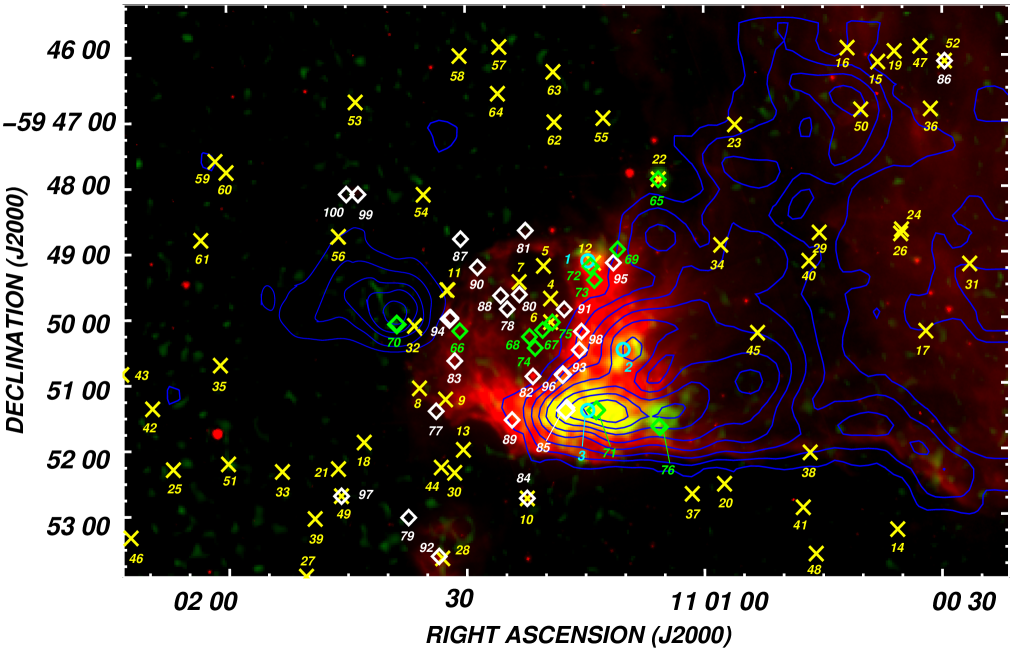
Figure 10: Composite image of NGC 3503 and its environs. Red colour shows the IRAC-GLIMPSE emission at 8.0 $\mu$m, while green/yellow tonalities show the ATLASGAL 870 $\mu$m continuum emission. The ¹³CO(J=2$\rightarrow$1) emission line integrated in the velocity ranges from $-$27.8 to $-$23.7 km s^-1  and $-$17.1 to $-$15.3 km s^-1are shown in blue contours. Thick light blue circles indicate the position of the MSX CHii  region candidates, while yellow crosses depict the position of the 2MASS sources with IR excess. Green and white diamonds indicate the position of WISE Class-I and Class-II candidates YSOs, respectively. Numerical references of YSOs are based on Tables 5 and 6. The size of the symbols do not match the angular size of the sources.

We intend to study the star formation in the vicinity of NGC 3503  by detecting all the candidate YSOs (intrinsically reddened) and analyzing their position with respect to the dust, ionized gas, and molecular gas.

In this new analysis we have used again the 2 MASS catalog (Cutri et al., 2003), which provides detections in $J$, $H$ and $K_{s}$ bands, to search for point sources with infrared excess. We have selected only sources with signal-to-noise ratio (S/N) $>$ 10 (quality “AAA”) and followed the criteria of Comerón et al. (2005), to determine the parameter $q$ = ($J$ - $H$) - 1.83 $\times$ ($H$ - $K_{s}$). Then, sources with $q<$ $-$0.15 (i.e. sources with IR excess) were identified as candidate YSOs. In Table 5 we have listed the 2MASS candidate YSOs identified with the method explained above. For completeness, we have also included in the table the three MSX CHii region candidates reported in Paper I. For the sake of clarity, the numerical identification up to source #12 is compatible to that of Paper I. The spatial distribution of 2MASS and MSX sources is depicted in Fig. 10. As can be seen from this figure, from a total of 61 sources detected in the field, only 10 sources are projected onto the IR counterpart of NGC 3503 or its central cavity, namely: #4, #5, #6, #7, #8, #9, #11, #12, and #22 (for completeness, we have included in Fig. 10 all the 2MASS candidate YSOs detected in the studied area). Sources #4 to #12 were previously reported in Paper I, as possibly associated with the nebula. Sources #4, #5, #6, #7 are projected towards the central cavity of NGC 3503, and lay inside the radio continuum counterpart of the nebula (see Fig. 2) while sources #8, #9, and #11 lay onto the IR arc towards the eastern and northern sections of IR the nebula. Low-intensity radio continuum emission is also seen projected onto these sources (see Fig. 2). Source #22 is coincident with a point-like source detected in the four IRAC bands, and correlates with the emission at 870 $\mu$m of D6 (see Figs. 9 and 10) and clump C11, suggesting that this candidate YSO is buried in a “cocoon” of cold dust and dense gas. Its WISE counterpart can be classified as a Class-I candidate (source #65; see below). None of the above mentioned 2MASS sources are seen projected onto the molecular gas associated with the nebula at velocities between –27.8 to –23.7 km s^-1 or –17.1 to –15.3 km s^-1(see Fig. 10). 2MASS sources #15, #16, #29, #34, #38, #40, #45, and #50) appear projected onto the north-western and western borders of the molecular gas in the velocity range from –27.8 to –23.7 km s^-1far from the nebula, thus, a physical association with the molecular environment of NGC 3503 is uncertain. Source #32 is projected onto the molecular component at velocities between –17.1 to –15.3 km s^-1(clump C9).

Candidate YSOs are usually classified, according to their evolutionary phase, into two standard categories: 1) Class-I YSO which are young protostellar sources embedded in dense infalling envelopes of gas and dust, and 2) Class-II YSO which are pre-main-sequence sources whose emission originates mainly in dense optically thick diks around the protostar (candidate T Tauri stars). These sources exhibit an infrared excess that cannot be attributed to the ISM along the line of sight, but rather to the envelope and/or the disk surrounding the protostar. Class-III sources are usually referred to as pre-main-sequence (or main-sequence) field stars. With the aim of identifying new candidate YSOs associated with NGC 3503, we have included in our analysis photometric data from the Wide-field Infrared Survey Explorer (WISE; Wright et al. 2010) obtained from the IPAC database. This survey maps the whole sky in four bands centered at 3.4, 4.6, 12, and 22 $\mu$m. We have used the criteria of Koenig et al. (2012), biased against the youngest and least massive candidate YSOs, as follows:

Table 5: Candidate YSOs obtained from the 2 MASS and MSX point source catalogs.

Source	RA, Dec. (J2000)	MSX source	F8	F12	F14	F21
No	(h m s, ∘′″)		(Jy)	(Jy)	(Jy)	(Jy)
1	11 01 10.77, –59 49 13.9	G289.4859+00.1420	1.49250	1.8145	0.9005	0.3180
2	11 01 11.18, –59 50 34.3	G289.4993+00.1231	0.82699	1.4887	1.2237	4.3818
3	11 01 13.57, –59 51 21.9	G289.5051+00.1161	0.87911	2.8632	1.6759	5.6330
	RA, Dec. (J2000)	2MASS source	$J$	$H$	$K$
$\#$	(h m s, ∘′″)		(mag)	(mag)	(mag)
4	11 01 19.34, -59 49 42.2	11011934-5949422	13.277	13.047	12.806
5	11 01 20.21, -59 49 12.3	11012021-5949123	15.084	14.837	14.506
6	11 01 19.33, -59 50 03.7	11011933-5950037	14.539	14.100	13.696
7	11 01 23.29, -59 49 26.9	11012329-5949269	14.862	14.380	14.027
8	11 01 35.91, -59 51 03.7	11013591-5951037	15.237	14.592	14.106
9	11 01 32.63, -59 51 14.0	11013263-5951140	15.633	14.946	14.404
10	11 01 22.38, -59 52 44.9	11012238-5952449	12.747	11.744	10.836
11	11 01 32.38, -59 49 33.9	11013238-5949339	14.754	14.243	13.873
12	11 01 13.90, -59 49 09.9	11011390-5949099	14.888	13.661	12.827
13	11 01 30.41, -59 52 00.2	11013041-5952001	13.110	13.006	12.857
14	11 00 35.64, -59 53 14.1	11003564-5953141	15.385	14.976	14.512
15	11 00 38.07, -59 46 06.3	11003807-5946063	14.239	13.649	13.229
16	11 00 41.91, -59 45 53.5	11004191-5945535	15.421	14.638	14.128
17	11 00 32.05, -59 50 12.6	11003205-5950126	14.676	14.123	13.693
18	11 01 42.92, -59 51 52.9	11014292-5951529	15.091	14.775	14.497
19	11 00 35.99, -59 45 56.6	11003599-5945566	15.347	14.712	14.238
20	11 00 57.48, -59 52 32.2	11005748-5952322	15.124	14.855	14.472
21	11 01 46.19, -59 52 17.1	11014619-5952171	15.145	14.657	14.284
22	11 01 05.71, -59 47 53.4	11010571-5947534	15.142	12.941	11.305
23	11 00 56.09, -59 47 03.5	11005609-5947035	15.796	15.042	14.527
24	11 00 35.10, -59 48 39.7	11003510-5948397	14.950	14.499	14.114
25	11 02 07.01, -59 52 17.1	11020701-5952170	12.534	12.421	12.269
26	11 00 35.21, -59 48 43.5	11003521-5948435	15.413	14.571	14.017
27	11 01 50.30, -59 53 55.2	11015030-5953552	13.501	13.435	13.264
28	11 01 33.09, -59 53 39.4	11013309-5953394	15.326	14.602	14.097
29	11 00 45.46, -59 48 42.5	11004546-5948425	14.941	14.390	13.905
30	11 01 31.53, -59 52 21.1	11013153-5952211	14.358	14.177	13.985
31	11 00 26.52, -59 49 11.2	11002652-5949111	15.785	15.019	14.418
32	11 01 36.49, -59 50 06.5	11013649-5950065	15.528	14.928	14.352
33	11 01 53.25, -59 52 19.4	11015325-5952194	14.362	14.091	13.856
34	11 00 57.88, -59 48 53.6	11005788-5948536	15.784	15.092	14.447
35	11 02 00.99, -59 50 41.7	11020099-5950417	15.593	14.831	14.246
36	11 00 31.45, -59 46 49.3	11003145-5946493	14.796	13.869	13.266
37	11 01 01.56, -59 52 41.3	11010156-5952413	15.020	14.670	14.388
38	11 00 46.66, -59 52 03.7	11004666-5952037	15.245	14.724	14.246
39	11 01 49.19, -59 53 02.6	11014916-5953026	14.233	14.117	13.899
40	11 00 46.77, -59 49 08.3	11004677-5949083	14.713	14.509	14.121
41	11 00 47.55, -59 52 53.9	11004755-5952539	15.062	14.778	14.451
42	11 02 09.58, -59 51 21.2	11020958-5951212	14.368	13.942	13.624
43	11 02 12.42, -59 53 19.2	11021242-5953192	14.666	14.477	14.227
44	11 01 33.21, -59 52 16.2	11013321-5952162	14.667	14.421	14.131
45	11 00 53.27, -59 50 14.1	11005327-5950141	15.318	14.585	14.094
46	11 02 13.44, -59 50 49.5	11021344-5950495	14.549	14.443	14.244
47	11 00 32.75, -59 45 52.0	11003275-5945520	14.577	14.018	13.628
48	11 00 45.93, -59 53 36.3	11004593-5953363	13.534	13.232	12.983
49	11 01 45.83, -59 52 41.9	11014583-5952419	14.245	13.271	12.580
50	11 00 40.21, -59 46 50.0	11004021-5946500	10.339	10.258	10.085
51	11 02 00.06, -59 52 12.1	11020005-5952121	15.819	14.957	14.206
52	11 00 29.66, -59 46 05.5	11002966-5946055	13.880	12.898	12.177
53	11 01 43.81, -59 46 41.8	11014381-5946418	15.025	14.770	14.478
54	11 01 35.32, -59 48 06.6	11013532-5948066	14.097	13.781	13.520
55	11 01 12.65, -59 46 57.3	11011265-5946573	14.795	14.540	14.239
56	11 01 46.02, -59 48 44.6	11014602-5948446	13.965	13.863	13.653
57	11 01 25.70, -59 45 51.8	11012570-5945518	14.413	14.381	14.241
58	11 01 30.72, -59 45 59.9	11013072-5945599	13.575	13.327	13.071
59	11 02 01.50, -59 47 35.2	11020150-5947352	13.610	13.485	13.333
60	11 02 00.12, -59 47 45.5	11020012-5947455	14.893	14.482	14.131
61	11 02 03.37, -59 48 47.4	11020336-5948474	15.734	15.127	14.512
62	11 01 18.81, -59 47 00.8	11011881-5947008	15.467	14.630	14.039
63	11 01 18.92, -59 46 14.8	11011892-5946148	15.156	14.839	14.500
64	11 01 25.91, -59 46 34.5	11012591-5946345	14.337	14.136	13.938

Table 6: Candidate YSOs obtained from the WISE point source catalog.

Source	Class	RA, Dec. (J2000)	WISE source	[3.4]	[4.6]	[12.0]	[22.0]	Matching with
No		( h m s, ∘′″)		(mag)	(mag)	(mag)	(mag)	MSX and
								2MASS sources
65	I	11 01 05.73, -59 47 53.5	J110105.73-594753.5	9.574	8.360	5.252	2.904	$\#$ 22
66	I	11 01 30.79, -59 50 11.6	J110130.79-595011.6	12.473	11.446	6.191	5.443
67	I	11 01 20.38, -59 50 10.9	J110120.35-595010.9	12.500	11.435	6.332	3.443
68	I	11 01 22.08, -59 50 17.1	J110122.01-595017.1	13.019	11.657	6.277	2.017
69	I	11 01 10.86, -59 48 57.3	J110110.86-594857.3	11.708	10.446	5.400	2.790
70	I	11 01 38.74, -59 50 04.4	J110138.74-595004.4	13.295	11.985	8.423	4.506
71	I	11 01 13.50, -59 51 23.8	J110113.50-595123.8	8.839	7.820	3.518	0.195	$\sim$ $\#$ 3
72	I	11 01 14.33, -59 49 12.8	J110114.33-594912.8	9.465	8.460	3.535	0.440	$\#$ 12 and $\#$ 1
73	I	11 01 13.81, -59 49 25.5	J110113.81-594925.5	10.826	9.792	5.056	5.581
74	I	11 01 21.30, -59 50 27.3	J110121.30-595027.3	13.165	11.902	7.195	4.070
75	I	11 01 19.13, -59 50 03.9	J110119.13-595003.9	12.388	11.244	6.155	2.784	$\#$ 6
76	I	11 01 05.73, -59 51 39.2	J110105.73-595139.2	11.520	10.477	5.249	2.930
source	Class	RA, Dec. (J2000)	WISE source	[3.4]	[4.6]	[12.0]	[22.0]
$\#$		( h m s, ∘′″)		(mag)	(mag)	(mag)	(mag)
77	II	11 01 33.82, -59 51 24.7	J110133.82-595124.7	11.083	10.696	6.622	3.169
78	II	11 01 24.80, -59 49 51.6	J110124.80-594951.6	13.012	12.209	7.309	3.537
79	II	11 01 37.36, -59 53 01.9	J110137.36-595301.9	13.755	13.277	8.518	6.706
80	II	11 01 23.27, -59 49 38.3	J110123.27-594938.3	12.510	11.852	7.009	3.912
81	II	11 01 22.49, -59 48 39.8	J110122.49-594839.8	12.270	11.805	7.058	3.972
82	II	11 01 21.60, -59 50 53.3	J110121.60-595053.3	8.906	8.003	5.084	1.147
83	II	11 01 31.44, -59 50 38.8	J110131.44-595038.8	11.325	10.853	6.003	3.915
84	II	11 01 22.38, -59 52 44.8	J110122.38-595244.8	9.631	9.046	5.964	3.402	$\#$ 10
85	II	11 01 17.35, -59 51 22.1	J110117.35-595122.1	9.120	8.162	3.628	1.149
86	II	11 00 29.67, -59 46 05.5	J110029.67-594605.5	11.125	10.635	8.156	5.558	$\#$ 52
87	II	11 01 30.65, -59 48 47.4	J110130.65-594847.4	13.315	12.992	10.876	6.954
88	II	11 01 25.62, -59 49 39.3	J110125.62-594939.3	11.862	11.122	7.408	4.760
89	II	11 01 24.25, -59 51 33.1	J110124.25-595133.1	9.862	9.281	4.447	4.481
90	II	11 01 28.54, -59 49 13.4	J110128.54-594913.4	11.943	11.598	6.835	4.735
91	II	11 01 17.62, -59 49 52.0	J110117.62-594952.0	10.820	10.080	6.688	1.612
92	II	11 01 33.53, -59 53 37.5	J110133.53-595337.5	11.280	10.437	5.819	3.931	$\#$ 28
93	II	11 01 15.75, -59 50 29.3	J110115.75-595029.3	9.352	8.891	4.124	1.614
94	II	11 01 31.93, -59 49 59.2	J110131.93-594959.2	10.784	10.340	6.082	4.162
95	II	11 01 11.41, -59 49 09.6	J110111.41-594909.6	10.341	9.843	5.005	2.870
96	II	11 01 17.84, -59 50 52.4	J110117.84-595052.4	8.748	8.193	5.036	5.552
97	II	11 01 45.82, -59 52 42.0	J110145.82-595242.0	11.722	11.118	9.209	6.565	$\#$ 49
98	II	11 01 15.46, -59 50 12.4	J110115.46-595012.4	9.949	9.430	4.714	1.120
99	II	11 01 43.54, -59 48 06.1	J110143.54-594806.1	12.745	11.920	7.143	5.265
100	II	11 01 45.01, -59 48 06.0	J110145.01-594806.0	12.976	12.318	7.502	5.598

after removing contamination arising from background objects like galaxies (very red in [4.6]$-$[12]), broad-line active galactic nuclei (of similar colours as YSOs, but distinctly fainter) and resolved PAH emission regions (redder than the majority of YSOs), we identified infrared excess sources demanding that

$$\begin{array}[]{ll}[3.4]-[4.6]-\sigma_{1}&>0.25\\ [4.6]-[12.0]-\sigma_{2}&>1.0\par\end{array}$$

where [3.4], [4.6], and [12.0] are the WISE bands 1, 2, and 3 magnitudes, respectively, and $\sigma_{1}=\sigma([3.4]-[4.6])$ and $\sigma_{2}=\sigma([4.6]-[12.0])$ indicate the combined errors of [3.4]$-$[4.6] and [4.6]$-$[12.0] colors, added in quadrature. Class I sources are a sub-sample of this defined by

$$\begin{array}[]{ll}[3.4]-[4.6]&>1.0\\ [4.6]-[12.0]&>2.0\par\end{array}$$

(the rest are Class II objects). For the method explained above, we have considered sources with error in magnitudes lower than 0.2 mag in bands 1, 2, and 3.

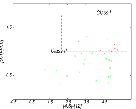
Figure 11: WISE band 1,2, and 3 color-color diagram showing the distribution of Class-I (in red) and Class-II (in green) candidate YSOs.

In Table 6 we list the candidate YSOs identified with the method explained above. For the sake of clarity, the numerical identification is succedent to that of Table 5. We found a total of 36 sources (12 Class-I and 24 Class-II candidates). In Fig.11 we show the WISE band 1,2, and 3 color-color diagram depicting the distribution of sources listed in Table 6. The spatial location of Class-I and Class-II candidates is illustrated in Fig. 10. Unlike 2MASS sources, the spatial distribution of WISE sources is rather concentrated toward the nebula. Sources #67, #68, #74, #75 (which is coincident with 2MASS source #6), #78, #80, #88, and #91 are projected toward the center of the nebula and its radio continuum emission (see Fig.2), while sources #66, #77, #81, #83, #90, and #94 are seen projected onto the IR arc. Sources #72 and #73 are almost coincident with the MSX CHii  region candidate #1 and 2MASS candidate YSO #12. Source #70 is projected close to the peak of emission of the molecular component at velocities between –17.1 to –15.3 km s^-1 (clump C9)

None of the WISE candidate YSOs sources mentioned so far are observed in the direction of any molecular clump detected in the velocity range from $-$27.8 to $-$23.7 km s^-1. Differently, three protostellar sources, #71, #76, and #85, are observed in the direction of ¹³CO emission peaks corresponding to clumps C4 and C3, which are the densest clumps (see Sect. 3.2). In order to better trace the spatial distribution of the gas/dust and candidate YSOs in this region, we present in Fig.12 a composite image of HCN, C¹⁸O, and 870 $\mu$m emission, superimposed on the location of WISE sources #71, #76, and #85. Sources #71 and #85 are projected onto dust clumps D2 and D1, respectively, and outwardly a C¹⁸O peak emission of seen at RA, Dec. (J2000) = (11^h01^m15^s, $-$59^∘51′20″) (C¹⁸O counterpart of clump C4). Source #85 is almost projected onto the HCN peak at RA, Dec. (J2000) = (11^h01^m16.7^s, $-$59^∘51′23″), while the position of source #71 is close to the HCN peak seen at RA, Dec. (J2000) = (11^h01^m11.6^s, $-$59^∘51′23.1″) and the central position of the MSX CHii  region candidate #3. This very likely suggests that these sources were formed inside high density molecular cores. As for source #76, this object is seen projected close to the direction of a C¹⁸O peak seen at RA, Dec. (J2000) = (11^h01^m2.5^s, $-$59^∘50′15″) (very likely the C¹⁸O counterpart of clump C3) and coincident with the dust clump D3 seen at 870 $\mu$m. This protostellar source is also projected onto the weaker HCN structure located at RA, Dec. (J2000) = (11^h01^m05^s, $-$59^∘51′40″). As suggested in Sect. 3.2, clump C4 is likely exposed to extra compression, heating, and ionization from NGC 3503 and SFO 62 , which might have triggered/enhanced the formation of protostellar candidates #71 and #85 (and probably #76) in the densest regions of the molecular gas. In that matter, it is also worth to stress the location of WISE sources #69, #82, #89, #93, #95, #96, and #98, which are spatially aligned perfectly following the eastern border of molecular clumps C4, C6, and C7. The location of these protostellar sources suggests that they are linked to the collected layers of molecular gas due to the expansion of the ionization front of NGC 3503 over its molecular environment, which has probably aided the stellar formation activity along the external borders of the molecular gas.

To determine whether the fragmentation of the collected layer via “collect and collapse” process might have triggered the star formation in the environs of NGC 3503, in Paper I we made use of the analytical model of Whitworth et al. (1994) for expanding Hii  regions. We obtained that $t_{\rm frag}$ $\sim$ 3.5 $\times$10⁶ yr and $R_{\rm frag}$ $\sim$ 7.5 pc, which are considerably larger than the age, $t_{\rm dyn}$, and size, $R_{\rm HII}$, of NGC 3503  (derived assuming a classical expanding Hii  region; Dyson & Williams 1997). This lead us to conclude that fragmentation of the collected layer triggered by the expansion of the nebula is doubtful. We keep in mind, however, that newer simulations have shown that accretion and ionization may occur simultaneously for compact Hii  regions, which makes their size unrelated on their age until late in their lifetimes (Peters et al., 2010).

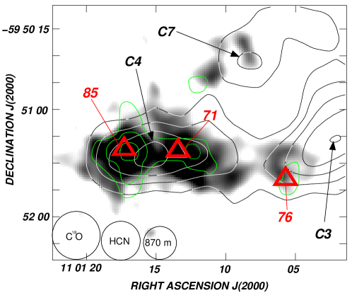
Figure 12: Composite image showing the emission of the HCN(J=3$\rightarrow$2) line (green contours), the C¹⁸O(J=2$\rightarrow$1) line (white/black contours), and the 870 $\mu$m continuum emission (grayscale) in the central region of NGC 3503. The velocity ranges are $-$26.2 to $-$25.2 km s^-1 and $-$26.5 to $-$25.5 km s^-1 for the C¹⁸O and HCN lines, respectively. Red triangles depict the position of WISE candidate YSOs #71, #76, and #85. The C¹⁸O couterpart of clumps C3, C4, and C7 are indicated. The beam sizes are shown in the lower left corner.

Given the lack of certainty of the latter scenario, we have considered alternative approaches: probably, the formation of YSOs lying at the border of the Hii  region (sources #69, #82, #89, #93, #95, #96, and #98) and inside clumps C4 and C3 (sources #71, #76, and #85) results from an interaction of the ionization front of NGC 3503 (and SFO 62 ) with pre-existing gravitationally bound molecular condensations (C3, C4, and C7; see Sect. 3.2), which has enhanced the formation of the protostellar objects (RDI process; Lefloch & Lazareff 1994). Also, the formation of the protostellar candidates may be the result of small-scale Jeans gravitational instabilities in the collected layers of molecular gas (e.g. Pomarès et al., 2009; Paron et al., 2011). Higher spatial resolution molecular observations might help to shed some light on these issues.

4 Summary

Using APEX CO(J=2$\rightarrow$1), ¹³CO(J=2$\rightarrow$1), C¹⁸O(J=2$\rightarrow$1), and HCN(J=3$\rightarrow$2) line data, and ATLASGAL 870 $\mu$m images, we carried out a multifrequency study of the molecular gas and dust associated with the Hii  region/star forming region NGC 3503. To analyze the star formation process in the region we made use of the WISE and 2MASS data obtained from the IPAC archive. This work is a follow-up study of Duronea et al. (2012). The main results can be summarized as follows:

1. The ionized gas of NGC 3503  is expanding against the molecular gas component in the velocity range from $\sim$ $-$28 to $-$23 km s^-1. The morphology of the molecular gas close to the nebula, the location of the PDR, and the shape of radio continuum emission confirm the “champagne flow” scenario proposed in Paper I.

2. New APEX observations allowed the small scale structure of the molecular gas associated with the nebula (previously reported in Paper I) to be fully imaged. We identified several molecular clumps (C1 to C11) and studied their physical and dynamical properties to investigate the impact of the expanding nebula and/or the southern bright rimmed cloud SFO 62  onto the molecular gas.

3. We found that warmer clumps (C3, C4, and C7) are close to the Hii  region, which is indicative of an external heating source, most probably by photoionization of their surface molecular layers by the intense UV field of Pis 17. Warmer clumps are also denser, which suggests that they are submitted to an external compression due to the expansion of NGC 3503. These clumps are likely molecular gas of the parental cloud that has been swept up by the expansion of the ionization front and has been condensed. Clump C4 is also adjacent to SFO 62 , which might explain its highest temperature and density. A noticeable velocity gradient is detected in C4. This gradient may indicative of a kinematical disturbance, or else, be the consequence of two molecular cores at slightly different velocity that are not fully resolved in the carbon monoxide emissions.

4. Clumps located near to NGC 3503 also have the highest LTE and virialized masses. They also exhibit the highest $M_{\rm LTE}/M_{\rm vir}$ ratio (predominantly $>$1), which, according to the classical interpretation, indicates that they are gravitationally bound.

5. All molecular clumps exhibit line broadening beyond the thermal width, which possibly indicates that in some cases the line widths of the composite spectrum of the clumps have different velocities, rather than showing turbulence effects. Also, spatially unresolved process like ouflows, infall, accretion, etc. might be contributing in the broadening.

6. We have analyzed the 870 $\mu$m emission, characteristic of filaments and dense molecular cores. We detected emission only in the direction of clumps C3, C4, and C7. This is also indicative of high density gas.

7. We have presented some evidence of stellar formation in the region by detecting sources with IR excess. Unlike 2MASS candidate YSOs, WISE Class-I and Class-II candidates show a spatial distribution concentrated to the IR nebula. Several sources are detected along the external border of two of the densest molecular clumps (C4 and C7) which suggests that they might be formed in the compressed layers of molecular gas. Three sources are projected close to HCN, C¹⁸O, and 870 $\mu$m emission peaks (coincident with the position of clumps C4 and C3). This very likely indicates that they were born inside high density molecular cores, making clumps C4 and C3 excellent candidates to further investigate star formation with higher spatial resolution instruments like ALMA.

8. Since the dynamical age and fragmentation time derived for the molecular layer differ to the age and radius of the nebula (Paper I) we have excluded the “collect and collapse” scenario for the YSO formation. Instead, we have proposed here some alternative mechanisms, such as “radiative-driven implosion” in pre-existing gravitationally bound clumps (C3, C4, and C7), or small-scale Jeans gravitational instabilities in the swept-up layers of molecular gas.