Nonclassical polarization dynamics in classical-like states

Abstract

Quantum polarization is investigated by means of a trajectory picture based on the Bohmian formulation of quantum mechanics. Relevant examples of classical-like two-mode field states are thus examined, namely Glauber and SU(2) coherent states. Although these states are often regarded as classical, the analysis here shows that the corresponding electric-field polarization trajectories display topologies very different from those expected from classical electrodynamics. Rather than incompatibility with the usual classical model, this result demonstrates the dynamical richness of quantum motions, determined by local variations of the system quantum phase in the corresponding (polarization) configuration space, absent in classical-like models. These variations can be related to the evolution in time of the phase, but also to its dependence on configurational coordinates, which is the crucial factor to generate motion in the case of stationary states like those here considered. In this regard, for completeness these results are compared with those obtained from nonclassical $N00N$ states.

I Introduction

According to its standard definition bornwolf-bk , light polarization refers to the ellipse described in time by the real component of the electric-field vector of a harmonic wave. Hence partial polarization can then be understood as the rapid and random succession of more or less different polarization states. In the quantum realm, we find that the electric field can never display a well-defined ellipse, just in the same way that particles cannot follow definite trajectories S1 ; S2 ; S3 ; S4 ; S5 . This is because the (field) quadratures satisfy the same commutation relations of position and linear momentum, and brings in several remarkable consequences: (i) there is no room for the classic, textbook definition of polarization, (ii) the simple and elegant picture of partial polarization as a random succession of definite ellipses gets lost, and (iii) any quantum light state is partially polarized because of unavoidable (quantum) fluctuations. The purpose of this work is to investigate whether these inconvenient quantum consequences can be overcome resorting to the Bohmian picture of quantum mechanics.

Polarization is a preferential laboratory for the analysis and application of fundamental aspects of the quantum theory. In this regard, one can get profit from tools coming from the latter to analyze optical behaviors. This is the case, for instance, when we consider the Bohmian formulation of quantum mechanics A ; sanz-AOP , which allows us to introduced suitable well-defined trajectories into the domain of quantum optics without violating any fundamental principle. Bearing this in mind, here we address the question of whether the set of trajectories determined by the Bohmian picture can still provide a reliable representation of polarization for quantum light states as an ensemble of electric-field trajectories. This would provide us with a rather intuitive model to understand quantum light closer to the original idea of polarization.

Recently the trajectories described by the electric field of one-photon two-mode states have been determined by following this approach LS13 . Here we extend the analysis to more relevant examples of classical-like two-mode field states, namely as Glauber and SU(2) coherent states CS ; SU2-1 ; SU2-2 . We specifically focus on this kind of states because a priori one might naively expect that they would constitute the appropriate arena to disclose the statistical description of polarization we are looking for. Surprisingly, we have found that for all these examples of classical-like light the electric-field trajectories are clearly incompatible with classical electrodynamics. Actually, for the SU(2) states we have found that they are far away from even resembling ellipses. For completeness, these results are compared to polarization trajectories associated with highly nonclassical stationary field, such as $N00N$ states.

The two-dimensional harmonic oscillator has been considered as a working model in previous Bohmian analyses holland-bk ; A2 , although it is typically associated with matter waves. Notice that the Bohmian approach is traditionally linked to quantum mechanics, and only recently it has also been used in problems involving electromagnetic fields (photons) – even if in the 1970s and 1980s a few authors already considered the possibility to extend the Bohmian approach to electromagnetic fields. However, in the area of quantum polarization, which we consider here, it has been little exploited as an analysis working tool. Here we report on an intriguing result, namely that Bohmian trajectories may reveal nonclassical polarization dynamics displayed by polarization field states that universally regarded as classical.

This work has been organized as follows. In Section II we present the prescriptions to define polarization trajectories as well as a discussion on the influence of singular points on the polarization dynamics. The dynamics associated with the polarization trajectories for coherent, classical-like states are reported and discussed in Section III, while in Section IV we deal with the counterpart for nonclassical $N00N$ states. To conclude, a series of final remarks are summarized in Section V.

II Polarization trajectories

II.1 Wave function for the electric field

Usually the Bohmian formulation of quantum mechanics is applied to the evolution of a particle in its position (configuration) space, which involves the wave function in the corresponding coordinate representation. In this work we make an effective transfer of this formulation to the evolution of a two-mode electric field, which involves the corresponding wave function for the field variables. Fortunately, such a transition is quite simple and straightforward, since each field mode is formally equivalent to a mechanical harmonic oscillator.

To take advantage of that equivalence in the simplest terms, we recall that a one-dimensional mechanical harmonic oscillator of mass $M$ with Hamiltonian

$$H=\frac{p^{2}}{2M}+\frac{1}{2}kq^{2},$$ (1)

with $q$ and $p$ being its position and linear momentum. This Hamiltonian can be quite conveniently described in terms of the dimensionless creation $b^{\dagger}$ and destruction $b$ operators, defined as

$$b=\sqrt{\frac{k}{2\hbar\omega}}\ \!q+i\frac{p}{\sqrt{2\hbar\omega M}},$$ (2)

with $\omega=\sqrt{k/M}$, and that satisfy the commutation relation $[b,b^{\dagger}]=1$, so that $H=\hbar\omega(b^{\dagger}b+1/2)$.

Likewise, a quantum one-mode electric field of frequency $\omega$ can be readily described by the complex amplitude operator $a$ as $E\propto a\exp(-i\omega t)$ in the complex representation. The operators $a$ and $a^{\dagger}$ satisfy the same commutation relation of $b$ and $b^{\dagger}$, this is $[a,a^{\dagger}]=1$. Regarding the real and imaginary parts of $E$, the following quadrature operators are defined

$$X=\frac{1}{\sqrt{2}}\left(a+a^{\dagger}\right),\quad Y=\frac{i}{\sqrt{2}}\left(a^{\dagger}-a\right),$$ (3)

which satisfy the commutation relation $[X,Y]=i$. These operators can be regarded, respectively, as the field counterparts of the mechanical position $q$ and linear momentum $p$ operators. This allows us to introduce the quadrature representation of any one-mode field state $|\psi\rangle$ as $\psi(x)=\langle x|\psi\rangle$ in terms of the eigenstates $|x\rangle$ of the quadrature operator $X$, where $X|x\rangle=x|x\rangle$. In this representation the quadrature operators become $X\psi(x)=x\psi(x)$ and $Y\psi(x)=-i\partial\psi(x)/\partial x$.

After Eqs. (2) and (3) the equivalence between the mechanical oscillator and the field mode can be carried out in very simple terms if we take units in which $\hbar=m=\omega=1$. For example, the free-field Hamiltonian reads $H=a^{\dagger}a+1/2$. More importantly, we can easily construct the wave functions for the number states $|n\rangle$ and the coherent states $|\alpha\rangle$, defined by the eigenvalue equations

$$a^{\dagger}a|n\rangle=n|n\rangle,\qquad a|\alpha\rangle=\alpha|\alpha\rangle,$$ (4)

in terms of their mechanical counterparts after Eqs. (4.1.32) and Eqs. (4.3.41) in Ref. GZ as

$$\psi_{n}(x)=\langle x|n\rangle=\frac{1}{\sqrt{2^{n}n!\sqrt{\pi}}}\ \!H_{n}(x)e^{-x^{2}/2},$$ (5)

where $H_{n}$ are the corresponding Hermite polynomials, and

$$\psi_{\alpha}(x)=\langle x|\alpha\rangle=\left(\frac{1}{\pi}\right)^{1/4}e^{-(x-\tilde{x})^{2}/2}e^{i\tilde{y}x},$$ (6)

where $\sqrt{2}\alpha=\tilde{x}+i\tilde{y}$. Both expressions can be easily derived from the the eigenvalue equations (4) and the differential form of the couple-amplitude operator $a\rightarrow(x+\partial/\partial x)/\sqrt{2}$ in the quadrature representation $\psi(x)$.

After this transformation from quantum mechanics to quantum optics, the only care to be taken is to remember that here $x$ does not represent a position, but the electric field in the form of the field quadrature $X$. This allows us the following fruitful translation to polarization of the Bohmian formulation of the evolution of a two-dimensional harmonic oscillator.

II.2 Polarization guidance equation

In analogy to the Bohmian formulation of quantum mechanics or, in short, Bohmian mechanics A , polarization trajectories described by the transverse electric field for two-mode harmonic light can be obtained by solving the guidance equation LS13

$$\dot{\bm{x}}={\bf\nabla}S,$$ (7)

where $\bm{x}=(x_{1},x_{2})$ denote the real, transverse components of the electric-field strength in Cartesian coordinates, $S$ is the phase of the field-state wave function in quadrature representation, and the gradient ${\bf\nabla}S$ is taken with respect to $\bm{x}=(x_{1},x_{2})$. Notice that, as in the usual Bohmian formulation, we have recast the electric field wave function in polar form,

$$\psi(\bm{x},t)\equiv\langle\bm{x}|\psi(t)\rangle=\left|\psi(\bm{x},t)\right|e^{iS(\bm{x},t)},$$ (8)

where we have assumed the field state $|\psi(t)\rangle$ to be pure, and $|\bm{x}\rangle=|x_{1}\rangle|x_{2}\rangle$ represents the eigenstates of the corresponding quadrature operators.

Notice that because light polarization just describes the time-evolution of the electric field, its configuration space is given by the electric-field variables $(x_{1},x_{2})$, which play the same role as the coordinates $\bm{r}$ in the case of particle dynamics. Once the general guidance equation is established, sets of polarization trajectories are determined by plugging the corresponding quantum field state (its phase) into this equation, and then solving it for some particular set of initial conditions, as in classical mechanics.

It is worth pointing out that in the quantum case all the information about the polarization state is encoded in the scalar wave function $\psi(\bm{x},t)$. More importantly, since $\psi(\bm{x},t)$ represents a probability amplitude, its phase has no classical analog. Therefore everything about the polarization trajectories relies on a nonclassical object, and hence we should expect that most conclusions derived from the phase of $\psi(\bm{x},t)$ will have no classical counterpart at all.

II.3 Equilibrium points

Except for the Glauber coherent states, here we have essentially focused on stationary states, and hence the topology of their phase in the polarization configuration space is going to be time-independent. This means that any motion will be associated with this topology rather than with the time-evolution of the phase gradient, as shown in LS13 . In this case, the mathematical framework of the stability theory is of much interest, for it may allow us to elucidate dynamical properties by identifying possible equilibrium points jordan-bk . This points are going to determine the behavior of the polarization trajectories in their vicinity and, therefore, the general dynamical landscape associated with each quantum state.

The nodes or zeros of the wave function, where $\psi(\bm{x})=0$ and the phase $S$ is undefined, constitute the first kind of candidate to equilibrium point. As is well known berry1 ; berry2 ; berry3 , nodes or phase singularities organize the global spatial structure of the flow of an optical field. This follows from Stoke’s theorem, which states that unless the curl of certain vector field is 0 within a certain region (irrotational flow), the line integral around a closed loop enclosing such a region (i.e., the circulation of such a vector field) will be nonzero. If this vector field is identified with the phase gradient, then we know that this quantity will be invariant under the addition to the phase of any integer multiple of $2\pi$. Consequently, if the curl of $\nabla S$ is nonzero, its circulation will be quantized. This is precisely what we observe in the case of Bohmian trajectories that whirl around a node of the wave function hirsch-1 ; hirsch-2 ; asanz-v1 ; asanz-v2 , where the quantization is in terms of integer multiples of $2\pi\hbar$. Of course, this also holds for the polarization trajectories that we are dealing with here, since

$$\oint\dot{\bm{x}}\cdot d\bm{x}=\oint dS=2\pi\sigma.$$ (9)

As it can be inferred from the latter integral, the presence of zeros in the wave function allows the introduction of a circulation number or topological charge, $\sigma$. This number has to be an integer, since the line integral provides the change experienced by the phase after an excursion returning to the original point Be ; merzbacher ; riess-1 ; riess-2 . Or, in topological terms, it accounts for the number of jumps between different equivalent points of the Riemann surface described by the logarithm of the wave function. In all cases examined in this work, the trajectories around the zeros will be nearly circular in a neighborhood of the node, giving rise to a vortical dynamics hirsch-1 ; hirsch-2 ; asanz-v1 ; asanz-v2 ; Be . It is worth noting that in quantum mechanics, it was Dirac who first noticed this effect dirac , suggesting the existence of magnetic monopoles. The concept of magnetic monopole has been further developed in the literature within the grounds of quantum hydrodynamics bialynicki . On the other hand, recently it has also been possible to recreate in laboratory conditions Dirac’s monopoles making use of the properties displayed by different materials, such as crystals made of spin ice monopole-2009-1 ; monopole-2009-2 ; monopole-2009-3 ; monopole-2009-4 or Bose-Einstein condensates of rubidium atoms monopole-2014 . Or course, strictly speaking, these are not elementary monopoles, but quasi-particles arising as an emergent phenomenon associated with a collective behavior, which display analogous properties to the hypothesized Dirac monopole.

Critical or stationary points, i.e., points at which all partial derivatives of a given function are zero, constitute the second kind of equilibrium point that we may identify. In our particular context, stationary points $\bm{x}_{s}$ will produce a vanishing phase gradient, i.e., ${\bf\nabla}S=0$. That is, given the guidance equation (7), we will find

$$\frac{d^{r}\bm{x}}{dt^{r}}\bigg{\arrowvert}_{\bm{x}=\bm{x}_{s}}={\bf 0}$$ (10)

for all $r>0$. In all the cases examined in this work, the trajectories near these points are hyperbolic, with the corresponding value of $\bm{x}_{s}$ being a saddle point of the velocity field ${\bf\nabla}S$. We have found no maxima or minima of $S$, which would lead respectively to sinks and sources of trajectories.

It is worth noticing that both nodes and stationary points are zeros of the current density, $\bm{j}=|\psi|^{2}\nabla S={\rm Im}\left(\psi^{\ast}{\bf\nabla}\psi\right)$. Nonetheless, the role played by these two types of equilibrium points is different. The asymptotically stable and unstable branches associated with the stationary points define separatrices around the nodes, which determine domains with different dynamical behavior. In particular, the direction of the flow around the nodes changes the sign when one passes from the domain of one of these nodes to another adjacent one. As it will be seen below, in some cases these domains are included within a larger domain with a preferential flow direction, while in others the full configuration space is totally divided in domains without enabling the appearance of larger domains.

III Field trajectories for classical-like states

III.1 Glauber coherent states

Two-mode quadrature coherent states, typically known as Glauber coherent states and denoted as $|\alpha_{1},\alpha_{2}\rangle$, constitute the paradigm of classical light. Their electric-field wave function after Eq. (6) is in this two-mode field scenario:

$$\psi(\bm{x},t)\propto e^{-\left(\bm{x}-\bm{\tilde{x}}\right)^{2}/2}e^{i\bm{\tilde{y}}\cdot\bm{x}},$$ (11)

where $\bm{\tilde{x}}$ and $\bm{\tilde{y}}$ are real two-dimensional vectors defined according to the relation $\sqrt{2}\bm{\alpha}e^{-it}=\bm{\tilde{x}}+i\bm{\tilde{y}}$, being $\bm{\alpha}=(\alpha_{1},\alpha_{2})$. Thus these vectors evolve in time as

$$\tilde{x}_{\ell}=\sqrt{2}|\alpha_{\ell}|\cos(t-\delta_{\ell}),\quad\tilde{y}_{\ell}=-\sqrt{2}|\alpha_{\ell}|\sin(t-\delta_{\ell}),$$ (12)

with $\delta_{\ell}=\arg{\alpha_{\ell}}$ for $\ell=1,2$. Since the phase is $S=\bm{\tilde{y}}\cdot\bm{x}$ the guidance equation is simply $\dot{\bm{x}}=\bm{\nabla}S=\bm{\tilde{y}}$, which can be easily solved analytically to give

$$x_{\ell}(t)=x_{\ell}(0)+\sqrt{2}|\alpha_{\ell}|\cos(t-\delta_{\ell})-\sqrt{2}|\alpha_{\ell}|\cos\delta_{\ell},$$ (13)

this is to say

$$\bm{x}(t)-\bm{x}(0)=\bm{\tilde{x}}(t)-\bm{\tilde{x}}(0).$$ (14)

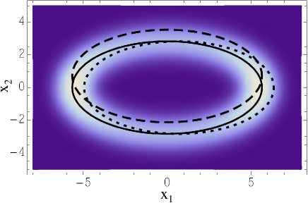
Figure 1: Polarization trajectories for a two-mode coherent state with $\alpha_{1}=4$ and $\alpha_{2}=2i$. The contour-plot represents the probability density associated with the one-cycle averaged probability distribution for the electric field $\overline{P}(\bm{x})$.

In Fig. 1 we have plotted three polarization trajectories for a Glauber coherent state by considering different initial conditions in Eq. (13). The solid line represents the most probable trajectory, starting at $t=0$ at the maximum of (11), i.e., $\bm{x}(0)=\bm{\tilde{x}}(0)$ so that $\bm{x}(t)=\bm{\tilde{x}}(t)$; the other two trajectories (dashed and dotted lines) start from points at one standard deviation from the maximum. The background represents a contour-plot of the probability density associated with the one-cycle averaged probability distribution for the electric field

$$\overline{P}(\bm{x})\propto\int_{0}^{2\pi}\left|\psi\left(\bm{x},t\right)\right|^{2}dt.$$ (15)

As happens with the Bohmian trajectories of a quantum harmonic oscillator, here we also notice that any trajectory associated with a Glauber state displays the same topology and keeps a constant distance with respect to the most probable one, as it is inferred from Eq. (14). In this case, this topology coincides with the polarization ellipse of a classical harmonic wave with complex-amplitude vector $\bm{\alpha}$. Nonetheless, only the most probable trajectory (the solid line in Fig. 1) is centered at the origin; any other trajectory will be slightly displaced, as mentioned before (see dashed and dotted lines in Fig. 1). Despite coherent states are regarded as typical examples of classical-like light, such a displacement constitutes an important difference with respect to what one would expect from classical electrodynamics, namely zero displacement (i.e., concentric trajectories).

III.2 SU(2) coherent states

The two-mode Glauber coherent states define another interesting family of classical-like states regarding polarization, namely the SU(2) coherent states. These states arise after recasting the two-mode Glauber coherent states as SU2-1 ; SU2-2

$$|\alpha_{1},\alpha_{2}\rangle=e^{-|\alpha|^{2}/2}\sum_{n=0}^{\infty}\frac{|\alpha|^{n}e^{in\delta}}{\sqrt{n!}}|n,\Omega\rangle.$$ (16)

Here $|n,\Omega\rangle$ denotes the SU(2) coherent state with $n$ photons, which reads explicitly as

$$|n,\Omega\rangle=\sum_{m=0}^{n}\begin{pmatrix}n\cr m\end{pmatrix}^{1/2}\cos^{m}\frac{\theta}{2}\sin^{n-m}\frac{\theta}{2}e^{-im\delta}|m,n-m\rangle,$$ (17)

where $|m,n-m\rangle$ are two-mode photon-number states, and (assuming $\alpha_{1}$ real without loss of generality)

$$\alpha_{1}=|\alpha|\cos\frac{\theta}{2},\qquad\alpha_{2}=|\alpha|\sin\frac{\theta}{2}\ e^{-i\delta}.$$ (18)

It is worth noting that the polarization state, as given by the Stokes parameters, is the same for the Glauber coherent states and all the SU(2) coherent states in Eq. (16).

The wave function $\psi(\bm{x},t)$ accounting for SU(2) coherence states with $n$ photons, given by Eq. (17), reads after Eq. (5) as

$$\psi(\bm{x},t)\propto\sum_{m=0}^{n}\frac{\alpha_{1}^{m}\alpha_{2}^{n-m}}{m!(n-m)!}H_{m}(x_{1})H_{n-m}(x_{2})e^{-\bm{x}^{2}/2}e^{-int}.$$ (19)

Here, the only analytical solution to the guidance equation holds in the particular case of $|\alpha_{1}|=|\alpha_{2}|$ and $\delta=\pm\pi/2$, for which we have $\psi(\bm{x})\propto\left(x_{1}\pm ix_{2}\right)^{n}e^{-\bm{x}^{2}/2}$. In this case, all trajectories are circles and there is only one node at the origin with charge $\sigma=\pm n$, the sign depending on the helicity of the classical polarization ellipse.

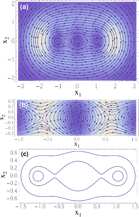
Figure 2: (a) Streamlines illustrating the trajectory dynamics associated with an SU(2) coherent state with $\alpha_{1}=4$, $\alpha_{2}=2i$, and $n=3$. The contour-plot represents the probability density $|\psi(\bm{x},t)|^{2}$ of the electric field. (b) Enlargement of panel (a) to show the dynamics around the central node and the two adjacent hyperbolic stationary points. (c) Four polarization trajectories showing the incompatibility with the classical electrodynamics of a freely evolving two-mode harmonic electric field.

This coincides exactly with the circular polarization associated with the complex-amplitude vector $\bm{\alpha}$. For any other general case, the trajectories shown in Fig. 2(a) provide an idea of the general trend. These trajectories, displayed in the form of streamlines (arrows indicate the directionality of the motion), correspond to an SU(2) coherent state with $\alpha_{1}=4$, $\alpha_{2}=2i$, and $n=3$; the contour-plot represents the probability density $|\psi(\bm{x},t)|^{2}$ associated with the coherent state considered. This example illustrates without loss of generality the results we have found for all cases examined, specifically that there are $n$ nodes located along the major axis of the classical ellipse associated with the complex vector $\bm{\alpha}$. In the vicinity of the nodes, the trajectories are nearly circular Be , as can be better seen in the enlargement around the central node provided in Fig. 2(b). The three nodes have the same topological charge $\sigma=+1$. Between any two consecutive nodes, along the line connecting them, there are $n-1$ hyperbolic stationary points jordan-bk . In the vicinity of these points, the trajectories display a hyperbolic topology with identical semi-axes [see Fig. 2(b)].

The trajectory that passes just through the two stationary points is a separatrix, which separates the three dynamical domains associated with each note from a single outer domain, where the trajectories move around the all three nodes. Actually, far from the nodes the trajectories approach circles. This can be readily shown analytically by considering the approximation $H_{n}(x)\approx(2x)^{n}$ for large $x$, and substituting it into the wave function (19), which yields

$$\psi(\bm{x})\propto\left(\bm{\alpha}\cdot\bm{x}\right)^{n}e^{-\bm{x}^{2}/2},$$ (20)

and hence $\dot{\bm{x}}\propto(x_{2},-x_{1})$, $\dot{\bm{x}}\cdot\bm{x}=0$, and $|\bm{x}|={\rm constant}$ along each trajectory, which define a circular motion. Of course, the rotation of the outer trajectories the three central domains can be associated with the motion around a single effective node of charge $|\sigma|=n$. As an illustration of the extremely streaking behavior displayed by the polarization trajectories associated with these classical-like polarization states, a representative set of them is shown in Fig. 2(c). As is apparent, the behavior exhibited by all these trajectories is clearly incompatible with the classical electrodynamics corresponding to a freely evolving two-mode harmonic electric field.

IV Nonclassical field: $N00N$ states

For the sake of comparison, we will also briefly consider a paradigm of nonclassical state, namely a $N00N$ state. These states constitute the polarization analog of Schrödinger cat states or coherent superpositions of distinguishable states. In the photon-number basis they read N00N-1 ; N00N-2 ; N00N-3 ; N00N-4 as

$$|\psi\rangle\propto\alpha_{1}|n,0\rangle+\alpha_{2}|0,n\rangle.$$ (21)

This can be regarded as an alternative quantum version of the coherent superposition of two orthogonal oscillations, which is the actual origin of polarization. The corresponding wave function is

$$\psi(\bm{x})\propto\left[\alpha_{1}H_{n}(x_{1})+\alpha_{2}H_{n}(x_{2})\right]e^{-\bm{x}^{2}/2}.$$ (22)

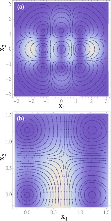
Figure 3: (a) Streamlines illustrating the trajectory dynamics associated with a $N00N$ state with $\alpha_{1}=4$, $\alpha_{2}=2i$, and $n=3$. The contour-plot represents the probability density $|\psi(\bm{x},t)|^{2}$ of the electric field. (b) Enlargement of panel (a) to show the dynamics around one of the hyperbolic stationary points and the corresponding four adjacent nodes.

A global picture of the dynamics for $N00N$ states is provided in Fig. 3 (left) in terms of streamlines. To compare with the case analyzed in Section III, the values $\alpha_{1}=4$, $\alpha_{2}=2i$, and $n=3$ have been considered again. An enlargement showing the dynamical details in the vicinity of one of the hyperbolic stationary points and the adjacent nodes can be seen in the right panel. The nodes form an array of $n\times n$ domains, where the trajectories are nearly circles with $\sigma=\pm 1$. In this case, the sign of $\sigma$ is always opposite for nearest neighbors. On the other hand, the stationary points form a $(n-1)\times(n-1)$ array, such that the corresponding separatrices divide the configuration space into isolated domains regardless of how far we find from the nodes. These points are located along the diagonals connecting nodes with the same sign of $\sigma$ and, again, the trajectories in their vicinity display a hyperbolic topology.

V Final remarks

We have addressed a Bohmian approach to light polarization in quantum optics A ; sanz-AOP ; LS13 by computing the trajectories described by the electric field of some classical-like two-mode states. In general, we have noticed that for Glauber coherent states all trajectories have the same elliptic form of the mean field, even if they are not centered at the origin. To some extent, this was an expected result. However, for SU(2) coherent states, the corresponding trajectories are further away from being ellipses. This can be ascribed to the fact that, although SU(2) coherent states are stationary, they are still able to exhibit a trajectory dynamics due to local phase variations, i.e., to a purely geometric origin, as previously shown in the case of single-photon superpositions LS13 .

Now, what is really quite remarkable here is the fact that polarization trajectories may display a dynamics far beyond the expected classical elliptical trajectories, even in the case of polarization field states that are universally regarded as classical. Instead, the results reported show that many different trajectories, with very different topologies, are compatible with every single state, which is in compliance with some recent quantum-polarization approaches, where the degree of polarization can never reach unity S3 ; rap1 ; rap3 ; rap4 .

In principle, these new results should be observable in practice in virtue of the close relationship between the Bohmian picture of quantum dynamics and the concept of weak measurement wm1 ; wm2 ; wm3 . Notice that this connection has already been proven experimentally in benchmark experiments be1 ; be2 . Furthermore, it has also been adapted to the case where the Bohmian trajectories hold in the field-quadrature space by means of the homodyne scheme, as shown in Ref. FF12 .

As shown here, the strange dynamics reported for SU(2) coherent states is primarily determined by the equilibrium points of the electric-field wave function, in particular a web of vortices. Analogously, this geometrical nature has also been observed in nonclassical light. This naturally leads to the issue of Bohmian chaos ABM , which is absent in all cases analyzed here, because vortices need to be evolving in time. In 1995 Parmenter and Valentine PV showed that just a linear superposition of eigenstates of a 2D anisotropic harmonic oscillator might lead to chaos under some specific conditions, an idea that Makowski and Frackowiak MF further analyzed later on in 2001, identifying the “simplest non-trivial model of chaotic Bohmian dynamics”. Nonetheless, the link between Bohmian chaos and vorticality was first established by Frisk in 1997 frisk , and more recently Wiskniacki, Pujals and Borondo WP ; WPB have found out that, in particular, it is the movement of vortices what induces the appearance of chaos, which explains why there are no signatures of chaos in our case. From a dynamical viewpoint, the states analyzed are all stable, although a slight perturbation would lead to motion of the observed saddle points and, therefore, to the appearance of chaos, although this is a subject that goes beyond the scope of the current work.

The above results, in contradiction with the type of dynamics that one would expect in principle from classical electrodynamics, constitute a quite remarkable issue, since such field states are universally regarded as classical-like concerning polarization. Nonetheless, there are some quantum approaches where these states also display nonclassical polarization features, as discussed in cnc-1 ; cnc-2 ; cnc-3 . In this regard, a natural question that arises here is whether there is any relationship between the manifestation of nonclassical polarization in these approaches and the one here discussed within the Bohmian framework. The answer is positive, there being a straightforward link between them. In terms of a mechanical-like language, the phase gradient in Eq. (7) provides the local value of a linear momentum. This can be suitably expressed as a local mean value of the momentum either via Wigner-Moyal phase-space distributions or Terletsky-Margenau-Hill ones lmv-1 ; lmv-2 ; lmv-3 ; lmv-4 ; lmv-5 ; WvT , which are the ones displaying nonclassical behavior in cnc-1 ; cnc-2 ; cnc-3 . Trajectories displaying strange behaviors might be then regarded as the result of quantum polarization distributions incompatible with classical physics.

From the above comments, it is clear that Glauber and SU(2) coherent states must be separately analyzed. The Wigner distribution for Glauber coherent states is classical (it is everywhere positive definite) and, consequently, one should go to nonlinear functions of the trajectories. This is because nonlinear local moments are related exclusively to Terletsky-Margenau-Hill WvT , which is nonclassical for Glauber coherent states cnc-1 ; cnc-2 ; cnc-3 . Regarding SU(2) coherent states, their characteristic trait is the presence of vortices governing the topology of the trajectories. These vortices arise when the amplitude of the wave function vanishes. This vanishing implies that both the Wigner and the Terletsky-Margenau-Hill distributions will be negative definite in regions around vortices. Roughly speaking, this means that the trajectories orbiting the vortices should be influenced by the nonclassical negative values of these distributions.

To conclude, we would like to stress the fact that the definition of the electric-field trajectories has no straightforward classical counterpart. There seems to be no simple classical analog for the phase of the electric-field wave function.

References

- (1) M. Born and E. Wolf, Principles of Optics (Cambridge University Press, Cambridge, UK, 1999), 7th ed.
- (2) S. De Bièvre, J. Phys. A 25, 3399 (1992).
- (3) J. Pollet, O. Méplan, and C. Gignoux, J. Phys. A 28, 7287 (1995).
- (4) A. Luis, Phys. Rev. A 66, 013806 (2002).
- (5) J. Liñares, M. C. Nistal, D. Barral, and V. Moreno, Eur. J. Phys. 31 991 (2010).
- (6) J. Liñares, D. Barral, M. C. Nistal, and V. Moreno, J. Mod. Opt. 58, 711 (2011).
- (7) A. S. Sanz and S. Miret-Artés, A Trajectory Description of Quantum Processes. I. Fundamentals (Springer, Berlin, 2012).
- (8) A. S. Sanz, M. Davidović, M. Božić, and S. Miret-Artés, Ann. Phys. 325, 763 (2010).
- (9) A. Luis and A. S. Sanz, Phys. Rev. A 87, 063844 (2013).
- (10) L. Mandel and E. Wolf, Optical Coherence and Quantum Optics (Cambridge University Press, Cambridge, UK, 1995); O. Giraud, P. Braun, D. Braun, Phys. Rev. A 78, 042112 (2008).
- (11) P. W. Atkins and J. C. Dobson, Proc. R. Soc. Lond. A 321, 321 (1971).
- (12) F. T. Arecchi, E. Courtens, R. Gilmore, and H. Thomas, Phys. Rev. A 6, 2211 (1972).
- (13) P. R. Holland, The Quantum Theory of Motion (Cambridge University Press, Cambridge, UK, 1993).
- (14) A. S. Sanz and S. Miret-Artés, A Trajectory Description of Quantum Processes. II. Applications (Springer, Berlin, 2014).
- (15) C. W. Gardiner and P. Zoller, Quantum Noise (Springer-Verlag, Berlin, 1991).
- (16) D. W. Jordan and P. Smith, Nonlinear Ordinary Differential Equations (Oxford University Press, Oxford, 1999), 3rd ed.
- (17) M. V. Berry, Singularities in Waves in Les Houches Lecture Series Session XXXV, ed. R. Balian, M. Kléman, and J.-P. Poirier (North-Holland, Amsterdam, 1981), pp. 453–543.
- (18) M. V. Berry, Wave Geometry: A plurality of singularities in Quantum Coherence, ed. J. S. Anandan (World Scientific, New York, 1991), pp. 92–98.
- (19) M. V. Berry and M. R. Dennis, Proc. R. Soc. A 457, 141 (2001).
- (20) J. O. Hirschfelder and A. C. Christoph, J. Chem. Phys. 61, 5435 (1974).
- (21) J. O. Hirschfelder, Ch. J. Goebel, and L. W. Bruch, J. Chem. Phys. 61, 5456 (1974).
- (22) A. S. Sanz, F. Borondo, and S. Miret-Artés, Phys. Rev. B 69, 115413 (2004).
- (23) A. S. Sanz, F. Borondo, and S. Miret-Artés, J. Chem. Phys. 120, 8794 (2004).
- (24) M. V. Berry, J. Phys. A 38, L745 (2005).
- (25) E. Merzbacher, Am. J. Phys. 30, 237 (1962).
- (26) J. Riess, Phys. Rev. D 2, 647 (1970).
- (27) J. Riess, Phys. Rev. B 13, 3862 (1976).
- (28) P. A. M. Dirac, Proc. R. Soc. Lond. A 133, 60 (1931).
- (29) I. Bialynicki-Birula and Z. Bialynicka-Birula, Phys. Rev. D 3, 2410 (1971).
- (30) D. J. P. Morris, D. A. Tennant, S. A. Grigera, B. Klemke, C. Castelnovo, R. Moessner, C. Czternasty, M. Meissner, K. C. Rule, J.-U. Hoffmann, K. Kiefer, S. Gerischer, D. Slobinsky, and R. S. Perry, Science 326, 411 (2009).
- (31) T. Fennell, P. P. Deen, A. R. Wildes, K. Schmalzl, D. Prabhakaran, A. T. Boothroyd, R. J. Aldus, D. F. McMorrow, and S. T. Bramwell, Science 326, 415 (2009).
- (32) S. T. Bramwell, S. R. Giblin, S. Calder, R. Aldus, D. Prabhakaran, and T. Fennell, Nature 461, 956 (2009).
- (33) H. Kadowaki, N. Doi, Y. Aoki, Y. Tabata, T. J. Sato, J. W. Lynn, K. Matsuhira, and Z. Hiroi, J. Phys. Soc. Jpn. 78, 103706 (2009).
- (34) M. W. Ray, E. Ruokokoski, S. Kandel, M. Möttönen, and D. S. Hall, Nature 505, 657 (2014); For completeness, see also the theoretical companion article: V. Pietilä and M. Möttönen, Phys. Rev. Lett. 103, 030401 (2009).
- (35) N. D. Mermin, Phys. Rev. Lett. 65, 1838 (1990).
- (36) J. J. Bollinger, W. M. Itano, D. J. Wineland, and D. J. Heinzen, Phys. Rev. A 54, R4649 (1996).
- (37) Ph. Walther, J.-W. Pan, M. Aspelmeyer, R. Ursin, S. Gasparoni, and A. Zeilinger, Nature 429, 158 (2004).
- (38) M. W. Mitchell, J. S. Lundeen, and A.M. Steinberg, Nature 429, 161 (2004).
- (39) A. P. Alodjants and S. M. Arakelian, J. Mod. Opt. 46, 475 (1999).
- (40) A. B. Klimov, L. L. Sánchez-Soto, E. C. Yustas, J. Söderholm, and G. Björk, Phys. Rev. A 72, 033813 (2005).
- (41) G. Björk, J. Söderholm, L. L. Sánchez-Soto, A. B. Klimov, I. Ghiu, P. Marian, and T. A. Marian, Opt. Commun. 283, 4440 (2010).
- (42) Y. Aharonov, D. Z. Albert, and L. Vaidman, Phys. Rev. Lett. 60, 1351 (1988).
- (43) Y. Aharonov and L. Vaidman, Phys. Rev. A 41, 11 (1990).
- (44) H. M. Wiseman, New J. Phys. 9, 165 (2007).
- (45) S. Kocsis, B. Braverman, S. Ravets, M. J. Stevens, R. P. Mirin, L. K. Shalm, and A. M. Steinberg, Science 332, 1170 (2011).
- (46) J. S. Lundeen, B. Sutherland, A. Patel, C. Stewart, and C. Bamber, Nature 474, 188 (2011).
- (47) J. Fischbach and M. Freyberger, Phys. Rev. A 86, 052110 (2012).
- (48) A. Benseny, G. Albareda, A. S. Sanz, J. Mompart, and X. Oriols, Eur. Phys. J. D 68, 286 (2014).
- (49) R. H. Parmenter and R. W. Valentine, Phys. Lett. A 201, 1 (1995); Erratum: Phys. Lett. A 213, 319 (1996).
- (50) A. J. Makowski and M. Frackowiak, Acta Phys. Pol. B 32, 2831 (2001).
- (51) H. Frisk, Phys. Lett. A 227, 139 (1997).
- (52) D. A. Wisniacki and E. R. Pujals, Europhys. Lett. 71, 159 (2005).
- (53) D. A. Wisniacki, E. R. Pujals, and F. Borondo, Europhys. Lett. 73, 671 (2006).
- (54) A. Luis, Phys. Rev. A 73, 063806 (2006).
- (55) L. M. Johansen, Phys. Lett. A 329, 184 (2004).
- (56) L. M. Johansen and A. Luis, Phys. Rev. A 70, 052115 (2004).
- (57) R. I. Sutherland, J. Math. Phys. 23, 2389 (1982).
- (58) K. K. Wan and P. J. Sumner, Phys. Lett. A 128, 458 (1988).
- (59) J. G. Muga, J. P. Palao, and R. Sala, Phys. Lett. A 238, 90 (1998).
- (60) B. J. Hiley, Found. Phys. 40, 356 (2010).
- (61) B. J. Hiley, J. Phys: Conf. Ser. 361, 012014 (2012).
- (62) A. Luis, Phys. Rev. A 67, 064101 (2003).