Arbitrary Transmission Power in the SINR Model:
Local Broadcasting, Coloring and MIS

Abstract

In the light of energy conservation and the expansion of existing networks, wireless networks face the challenge of nodes with heterogeneous transmission power. However, for more realistic models of wireless communication only few algorithmic results are known. In this paper we consider nodes with arbitrary, possibly variable, transmission power in the so-called physical or SINR model. Our first result is a bound on the probabilistic interference from all simultaneously transmitting nodes on receivers. This result implies that current local broadcasting algorithms can be generalized to the case of non-uniform transmission power with minor changes. The algorithms run in $\mathcal{O}(\Gamma^{2}\Delta\log n)$ time slots if the maximal degree $\Delta$ is known, and $\mathcal{O}((\Delta+\log n)\Gamma^{2}\log n)$ otherwise, where $\Gamma$ is the ratio between the maximal and the minimal transmission range. The broad applicability of our result on bounding the interference is further highlighted, by generalizing a distributed coloring algorithm to this setting.

1 Introduction

One of the most fundamental problems in wireless ad hoc networks is to enable efficient communication between neighboring nodes. This problem recently received increasing attention among the distributed algorithm community, as more refined models of wireless communication became established in algorithms research. Among these models, the so-called physical or signal-to-interference-and-noise (SINR) model is most prominent and promising, due to its common use in the engineering literature. However, so far most algorithmic work in the SINR model is restricted to the case of uniform transmission power. In this case, local broadcasting [8, 20, 22, 7] provides initial communication by enabling each node to transmit one message such that all intended receivers (i.e., neighbors) are able to decode the message.

In this work we consider the problem of local broadcasting in the SINR model under arbitrary transmission power assignment, i.e., each node has its individual, possibly variable, transmission power. We are the first to consider this setting from an algorithmic perspective. While some distributed node coloring algorithms do consider the transmission power to be variable [3, 21], they still increase the transmission power synchronously and thus effectively operate on an uniform power network. The sole line of research that leverages non-uniform transmission power is on link scheduling and capacity maximization [9, 11]. However, there, each node is usually considered to be either transmitter or receiver. If a node has multiple roles it might have to adapt its transmission power frequently. On the other hand, the effects of heterogeneous transmission power are considered in simulation-based studies for example in [6, 16], while the case of unidirectional communication links, which are a result of heterogeneous transmission powers, is studied even more frequently [23, 19].

We assume the harsh environment of an wireless ad hoc network just after deployment. In particular, we consider multi-hop networks, where the nodes do initially not have any information about whether other nodes are awake, have already started the algorithm or in which phase of the algorithm they are. The only knowledge they may have is an upper bound on the number of neighbors, and a rough bound on the total number of nodes in the network. Note that our model does not assume a collision detection mechanism. Additionally to this harsh model, we also considered some recent ideas regarding practical matters of algorithms for wireless networks by Kuhn et. al. [2]. They promoted the use of lower and upper bounds for important network parameters such as $\alpha,\beta$ and ${\operatorname{N}}$ (cf. Section 2). This is an important step towards practicability of the algorithms as upper and lower bounds to these values are well-represented in the literature, however, exact values vary depending on the network environment.

1.1 Contributions

In this work we are the first to consider arbitrary transmission powers in the SINR model, and thus networks with unidirectional links for the problems of local broadcasting, distributed node coloring and MIS. However, our first contribution is of more general nature and provides an abstract method for bounding the interference in these networks. We prove that transmissions are feasible based on the sum of local transmission probabilities. This result is widely applicable, as verifying that the sum of local transmission probabilities is bounded as required, is relatively simple.

Our second result transfers algorithms for local broadcasting presented in [8, 7] to the case of arbitrary transmission power assignment. We achieve local broadcasting in $\mathcal{O}(\Gamma^{2}\Delta\log n)$ time slots if the maximal degree $\Delta$ is known and $\mathcal{O}((\Delta+\log n)\Gamma^{2}\log n)$ otherwise, where $\Gamma$ is the ratio between the maximal and the minimal transmission range. Note that these bounds match those for the uniform case if the algorithms are run on such networks. Additionally we discuss the case of variable transmission power in Section 4.2, which achieves similar bounds, but allows nodes to change the transmission power in each time slot instead of fixing it for each round of local broadcasting.

Finally we give an algorithm for distributed node coloring in these harsh environments. The algorithm is in based on an algorithm by Moscibroda and Wattenhofer [12], which was adapted to the uniform SINR model by Derbel and Talbi [3]. Note however, that fundamental changes to the algorithm itself are required due to the increased complexity of the network structure, such as unidirectional communication links. We introduce a new network parameter $\ell$, that measures the length of the longest simple unidirectional chain in the partially directed network and prove that our distributed node coloring algorithm colors the network with $\mathcal{O}(\Gamma^{2}\Delta)$ colors in $\mathcal{O}((\Delta+\ell)\Gamma^{6}\Delta\log n)$ time slots. By simplifying the algorithm we obtain an algorithm that computes an MIS in $\mathcal{O}(\ell\Gamma^{4}\log n)$ time slots. Note that all our algorithms are fully operational in the unstructured radio network, especially under asynchronous node wake-up and sleep.

1.2 Related Work

The study of local broadcasting, and interference in general, has only recently emerged. Especially in classical distributed message passing models such as $\mathcal{LOCAL}$ or $\mathcal{CONGEST}$ [15], the transmission of a message to neighbors is guaranteed. However, this is not the case for wireless networks. Hence interference in general and local broadcasting in particular must be considered in the more realistic SINR model of interference. Goussevskaia et. al. [7] were the first to present local broadcasting algorithms in the SINR model. Their first algorithm assumes an upper bound $\Delta$ on the number of neighbors to be known by the nodes and solves local broadcasting with high probability in $\mathcal{O}(\Delta\log n)$ time, while the second algorithm does not assume this knowledge and requires $\mathcal{O}(\Delta\log^{3}n)$ time. The second algorithm has subsequently been improved by Yu et. al. to run in $\mathcal{O}(\Delta\log^{2}n)$ [22], and again to $\mathcal{O}(\Delta\log n+\log^{2}n)$ [20]. This bound has been matched by Halldórsson and Mitra in [8] using a more robust algorithm, along with an algorithm that leverages carrier sensing to achieve a time complexity of $\mathcal{O}(\Delta+\log n)$.

Research on distributed node coloring dates back to the first days of distributed computing nearly 30 years ago. Due to the wide variety of results in this area, we refer to the monograph recently published by Barenboim and Elkin [1] for results in the $\mathcal{LOCAL}$ model. Note that the considered message passing model abstracts away characteristics of a newly deployed wireless ad hoc network: Global interference, asynchronous node wake-up and sleep, and unidirectional communication links are not considered. Thus these algorithms cannot directly be used in the harsh model considered in this work.

An algorithm that colors the network with $\mathcal{O}(\Delta)$ colors in $\mathcal{O}(\Delta\log n)$ time was presented by Moscibroda and Wattenhofer in [13]. However, they assume a graph-based interference model. The algorithm has subsequently been improved in [12] and [17] and transfered to the SINR model by Derbel and Talbi [3] with the same bound on colors and runtime as the original algorithm. Yu et. al. consider the problem of coloring with only $\Delta+1$ colors in [21] and present algorithms that run in $\mathcal{O}(\Delta\log^{2}n)$ time slots or $\mathcal{O}(\Delta\log n+\log^{2}n)$ if the nodes transmission power can be tuned by a constant factor.

2 Preliminaries

We consider a wireless network consisting of $n$ nodes, that are placed arbitrarily on the Euclidean plane. We assume that all nodes in the network know their ID and an upper bound $\tilde{n}$ on $n$, with $\tilde{n}\leq n^{c}$ for some constant $c\geq 1$. As the upper bound influences our results only by a constant factor we usually write $n$ even though only $\tilde{n}$ may be known by the nodes. Also, we assume that nodes know lower and upper bounds on the transmission power or the transmission ranges. This assumption is realistic, as lower bounds for reasonable minimal transmission ranges can be computed while upper bounds (for specified frequencies) are often regulated by public authorities.

In the geometric SINR model a transmission from node $v$ to node $w$ is successful iff the SINR condition holds:

$$\frac{\frac{{\operatorname{P}}_{v}}{{\operatorname{dist}}(v,w)^{\alpha}}}{\sum_{u\in\mathcal{I}}\frac{{\operatorname{P}}_{u}}{{\operatorname{dist}}(u,w)^{\alpha}}+{\operatorname{N}}}\geq\beta$$ (1)

where ${\operatorname{P}}_{v}$ (${\operatorname{P}}_{u}$) denotes the transmission power of node $v$ ($u$), $\alpha$ is the attenuation coefficient, which depends on the environment and characterizes how fast the signal fades. The SINR-threshold $\beta\geq 1$ is a hardware-defined constant, ${\operatorname{N}}$ is the environmental noise and $\mathcal{I}$ is the set of nodes transmitting simultaneously with $v$. As introduced in [2] and motivated by the hardness of determining exact network parameters we restrict our nodes knowledge to upper and lower bounds of the values $\alpha$, $\beta$ and ${\operatorname{N}}$ and denote them by e.g. $\mkern 3.5mu\underline{\mkern-3.5mu\alpha\mkern-3.5mu}\mkern 3.5mu$ and $\bar{\alpha}$ for the minimal and maximal values.

Based on the SINR constraints, we define the maximum transmission range of a node $v$ to be $\bar{\operatorname{R}}_{v}=(\frac{{\operatorname{P}}_{v}}{\bar{{\operatorname{N}}}\bar{\beta}})^{1/\bar{\alpha}}$. Note that this is maximal under the restriction that this range can be reached regardless of the actual network parameters $\alpha$, $\beta$, ${\operatorname{N}}$. The global maximum transmission range in the network is denoted by $\bar{\operatorname{R}}$, the minimum range by $\mkern 3.5mu\underline{\mkern-3.5mu\operatorname{R}\mkern-3.5mu}\mkern 3.5mu$ and the ratio between $\bar{\operatorname{R}}$ and $\mkern 3.5mu\underline{\mkern-3.5mu\operatorname{R}\mkern-3.5mu}\mkern 3.5mu$ by $\Gamma=\frac{\bar{\operatorname{R}}}{\mkern 3.5mu\underline{\mkern-3.5mu\operatorname{R}\mkern-3.5mu}\mkern 3.5mu}$. Due to the SINR constraints, a node $v$ cannot reach another node $w$ which is located at the maximum transmission range of $v$, as soon $v$ transmits simultaneously with any other node in the network. As having only one simultaneous transmission in the network is not desired, we use a parameter $\delta>1$ to determine the distance up to which the nodes messages should be received. We call this distance the broadcasting range $\operatorname{R}_{v}=(\frac{{\operatorname{P}}_{v}}{\delta\bar{{\operatorname{N}}}\bar{\beta}})^{1/\mkern 3.5mu\underline{\mkern-3.5mu\alpha\mkern-3.5mu}\mkern 3.5mu}$ and the region within this range from $v$ the broadcasting region $B_{v}$. We denote the maximum number of nodes within the transmission range $\bar{\operatorname{R}}_{v}$ of any $v$ as $\Delta$. This is an upper bound on the number of nodes reachable from $v$, since the broadcasting range $\operatorname{R}_{v}$ is fully contained in the transmission range. Note that $\Delta$ is known by the nodes only if stated with the corresponding algorithms. We define the proximity region around $v$ as the area closer than $3\bar{\operatorname{R}}$ to $v$. Note that even though we use time slots in our analysis, we do not require a global clock or synchronized time slots in our algorithm. Decent local clocks are sufficient, while time slots are only required in the analysis.

Roadmap: In the following section we bound the probabilistic interference of nodes outside the proximity region based on the sum of transmission probabilities from within each transmission region. In Section 4 we apply this result to previous results on local broadcasting and thereby transfer current algorithms to the more general model. The applicability of our results is highlighted in Section 5, as we consider the problem of distributed node coloring and generalize a well-known algorithm from the case of uniform transmission powers. We conclude this paper in Section 6 with some final remarks.

Note that even though we use time slots in our analysis, we do not require a global clock or synchronized time slots in our algorithm. Decent local clocks are sufficient, while time slots are only required in the analysis.

Roadmap: In the following section we will bound the probabilistic interference of nodes outside the proximity region based on a bound on the sum of transmission probabilities from within each transmission region. In Section 4 we apply this result to previous results on local broadcasting and thereby transfer current algorithms to the more general model. In Section 5 we consider distributed node coloring and describe an algorithm that is capable of computing an $\mathcal{O}(\Gamma^{2}\Delta)$ coloring, or after a simplification an MIS. We conclude this paper in Section 6 with some final remarks.

3 Bounding the Interference

In contrast to other models for interference in wireless communication such as the protocol model, the SINR model captures the global aspect of interference and reflects that even interference from far-away nodes can add up to a level that prevents the reception of transmissions from relatively close nodes. To ensure that a given transmission can be decoded by all nodes within the broadcasting range, one usually proves that reception within a certain time interval is successful with high probability (w.h.p.—with probability at least $1-\frac{1}{n^{c}}$ for a constant $c>1$). Such a proof can be split in two parts

1. The probability that a node transmits within a proximity region around a sender is constant

2. Let $P_{\text{2high}}(v)$ be the event that the interference from all nodes outside of the proximity region of $v$ on nodes in the broadcasting region of $v$ is too high. Show that $P_{\text{2high}}(v)$ has constant probability.

We shall follow this scheme by considering the transmission of an arbitrary node and proving that both conditions hold with constant probability in each time slot, and hence a local broadcast is successful with high probability.

In order to make the result general and applicable to many different settings, we make only one very general assumption. Namely we assume the sum of transmission probabilities from within a broadcasting region to be bounded by a constant. This is very common and allows us to apply the analysis from this section in the following Sections 4 and 5 to generalize algorithms designed for the uniform transmission power case to the more general case considered in this paper.

Definition 1.

Given a network of $n$ nodes with at most $\Delta$ nodes in each transmission region. Let $\gamma$ be the upper bound on the sum of transmission probabilities from within one transmission region.

Let the upper bound on the sum of transmission probabilities from within each transmission region be

$$\gamma:=\frac{(\delta-1)}{120\bar{\beta}\Gamma^{2}\sum_{i=1}^{n}\frac{1}{i^{\bar{\alpha}-1}}}.$$ (2)

Note that this bound can be realized, for example by requiring nodes to transmit with probability $\gamma/\Delta$. Another option is the so-called slow-start technique, cf. Section 4.1.2. The constant is of the stated form, mainly to bound the interference from all other nodes in the network in the proof of Theorem 1. It holds that $\gamma\leq 1$. Let us now prove a bound on the probability that a close-by node transmits, which is also required for the main theorem of this section.

Lemma 2.

Given an arbitrary node $v$. The probability that no node in the proximity region transmits in a given time slot is at least $1/4$.

Proof.

Let $3\bar{\operatorname{R}}(v)$ denote the set of nodes that are closer to $v$ than $3\bar{\operatorname{R}}$ in this argument. This is the set of nodes in the proximity region of $v$. The probability that a node in $3\bar{\operatorname{R}}(v)$ transmits in a single time slots is

$$P_{\text{none}}^{3\bar{\operatorname{R}}(v)}\geq\prod_{u\in 3\bar{\operatorname{R}}(v)}\left(1-p_{u}\right)\geq\left(\frac{1}{4}\right)^{\sum_{u\in 3\bar{\operatorname{R}}(v)}p_{u}}\geq\left(\frac{1}{4}\right)^{49\Gamma^{2}\cdot\gamma}\geq\left(\frac{1}{4}\right),$$

where the second inequality holds due to Fact 1 from Appendix A.3, the third inequality due to a simple geometric argument about the number of independent nodes within distance $3\bar{\operatorname{R}}$ of $v$ and the bound on the sum of transmission probabilities from within each transmission region. The last inequality holds since $49\Gamma^{2}\cdot\gamma<1$. ∎

Let us now consider nodes that are not in the proximity region of the transmitting node. In order to bound the interference originating from these nodes, we use rings around the transmitting node and bound the probabilistic interference from within each ring. Note that although our definition of the proximity region and rings differ, similar arguments are made, for example, in [8, 7].

Definition 3.

For a node $v$, the ring $C_{i}^{v}$, $i\geq 0$, is defined as the set of nodes with distance at least $(i+1)\cdot\bar{\operatorname{R}}$ and at most $(i+2)\cdot\bar{\operatorname{R}}$. For a ring $C_{i}^{v}$, the extended ring $C_{i+}^{v}$ is defined as the set of nodes with distance at least $i\cdot\bar{\operatorname{R}}$ and at most $(i+3)\cdot\bar{\operatorname{R}}$.

Note that for a ring $C_{i}^{v}$, the extended ring $C_{i+}^{v}$ is defined such that the nodes in the transmission region of an arbitrary node $w\in C_{i}^{v}$ are contained in $C_{i+}^{v}$. If it is clear to which node $v$ the rings refer, we write $C_{i}$ and $C_{i+}$ for brevity.

Theorem 1.

Let the sum of transmission probabilities from each transmission region be upper bounded by $\gamma$. Given a node $v$, the probabilistic interference from nodes outside the proximity region of $v$ is upper bounded by $(\delta-1)N$.

Proof.

Let us first bound the interference from a single ring $C_{i}$. By a simple geometric argument it holds that the maximal number of independent nodes in the extended ring $C_{i+}$ is at most $(6i+9)\bar{\operatorname{R}}^{2}/\mkern 3.5mu\underline{\mkern-3.5mu\operatorname{R}\mkern-3.5mu}\mkern 3.5mu^{2}$. By combining this number with the sum of transmission probabilities from within each broadcasting region, we can bound the interference from the nodes in $C_{i}$. As each node in the ring $C_{i}$ has distance greater than $i\cdot\bar{\operatorname{R}}$ from any node in $B_{v}$, it follows that the probabilistic interference on any node $u\in B_{v}$ is at most

$$\Psi_{C_{i}} \leq\sum_{w\in C_{i+}}\frac{p_{w}{\operatorname{P}}_{w}}{(i\bar{\operatorname{R}})^{\bar{\alpha}}} \leq\frac{4(6i+9)\bar{\operatorname{R}}^{2}\gamma\bar{\beta}\bar{{\operatorname{N}}}}{\mkern 3.5mu\underline{\mkern-3.5mu\operatorname{R}\mkern-3.5mu}\mkern 3.5mu^{2}i^{\bar{\alpha}}}\cdot\left(\frac{\bar{\operatorname{R}}}{\bar{\operatorname{R}}}\right)^{\bar{\alpha}} \leq\frac{60\gamma\bar{\beta}\bar{{\operatorname{N}}}}{i^{\bar{\alpha}-1}}\cdot\left(\frac{\mkern 3.5mu\underline{\mkern-3.5mu\operatorname{R}\mkern-3.5mu}\mkern 3.5mu}{\bar{\operatorname{R}}}\right)^{2}.$$

Summing over all rings it follows

$$\Psi_{w\not\in 3\bar{\operatorname{R}}(v)} \leq\sum_{i=2}^{\infty}\Psi_{C_{i}}\leq 60\gamma\bar{\beta}\bar{{\operatorname{N}}}\Gamma^{2}\sum_{i=1}^{n}\frac{1}{i^{\bar{\alpha}-1}}\leq\frac{(\delta-1)\bar{{\operatorname{N}}}}{2},$$

where the second inequality holds by inserting the bound on $\Psi_{C_{i}}$ and the fact that there are at most $n$ non-empty rings. The last inequality follows from the upper bound on $\gamma$, stated in Equation 2. ∎

4 Local Broadcasting

In the previous section we have shown how to bound the probabilistic interference from nodes outside of the proximity region based on an upper bound on the sum of transmission probabilities from within each transmission region. Such bounds are known for many algorithms in the case of uniform transmission power, and hence we can plug our results into a large body of related work, and transfer results with minimal additional efforts to the case of arbitrary but fixed transmission power. In the following section we briefly state our results regarding local broadcasting along with proof sketches as required. In Section 4.2 we discuss our results regarding variable transmission power.

4.1 Arbitrary but Fixed Transmission Power

The current results on local broadcasting with the knowledge of $\Delta$ are based on transmitting with a fixed probability in the order of $1/\Delta$ for a sufficient number of time slots in $\mathcal{O}(\Delta\log n)$, while results that do not assume the maximal degree $\Delta$ to be known are usually based on a so-called slow-start mechanism.

4.1.1 With knowledge of the maximal degree $\Delta$

Let us first consider the case, in which each node knowns the maximal degree $\Delta$. Using the result on local broadcasting by Goussevskaia, Moscibroda and Wattenhofer [7], it is easy to show that local broadcasting can be realized in $\mathcal{O}(\Gamma^{2}\Delta\log n)$ time slots by simply adapting the transmission probability to our requirements.

Theorem 2.

Let the transmission probability of each node be $p=\gamma/\Delta$, and $c>1$ an arbitrary constant. A node $v$ that transmits with probability $p$ for $8c/p\log n=\mathcal{O}(\Gamma^{2}\Delta\log n)$ time slots successfully transmits to its neighbors whp.

Proof.

Since the transmission probability is chosen such that the sum of transmission probabilities from within each proximity range is at most $\gamma$, we can directly apply Theorem 1. Using the theorem, combined with the standard Markov inequality, the probability that the interference from nodes outside of the proximity region is too high (i.e., higher than $(\delta-1)\bar{{\operatorname{N}}}$) is less than $1/2$. Lemma 2 states that the probability that no node within the proximity range of a node transmits is greater than $\frac{1}{4}$. Combining both probabilities with the transmission probability of $p$ implies that the probability of a successful broadcast is at least $p/8$ in each time slot. Thus transmitting for $8c/p\log n$ time slots results in a successful local broadcast with probability at least $1-\frac{1}{n^{c}}$. A detailed proof can be found in Appendix A.1. ∎

4.1.2 Without knowledge of $\Delta$

Let us now consider the case that the nodes are not given a bound on the maximum degree $\Delta$. In contrast to the previous algorithm for local broadcasting, the “optimal” transmission probability is initially unknown.

In order to create local broadcasting algorithms for this model, a slow start mechanism can be used [8, 20, 22, 7]. In such a mechanism each node starts with a very low transmission probability in the range of $\mathcal{O}(1/n)$ and doubles the probability until a certain number of transmissions are received, and the probability is reset to a smaller value. With such a mechanism, local broadcasting in the (uniform-powered) SINR model can be achieved in $\mathcal{O}(\Delta\log n+\log^{2}n)$ [8, 20]. Although different forms of the slow start mechanisms are used they reset the transmission probabilities such that the sum of transmission probabilities in each transmission region can be upper bounded by a constant.

Let us now consider the algorithm of Halldórsson and Mitra, described in [8]. We can adapt the algorithm so that local broadcasting provably works with high probability in the more general model considered in this paper. This can be done by modifying the maximal transmission probability to be $\gamma/16$ instead of $1/16$, which can be done by simply changing Line 7 of Algorithm 1 in [8] from $p_{y}\leftarrow\min\{\frac{1}{16},2p_{y}\}$ to $p_{y}\leftarrow\min\{\frac{\gamma}{16},2p_{y}\}$. This minimal adaptation allows us to bound the sum of transmission probabilities similar to how it is done in the original paper.

Lemma 4.

Let $\mathcal{N}$ be a network with arbitrary transmission power assignment, asynchronous node wake-up and let all nodes execute Algorithm 1 from [8] with maximal transmission probability be set to $\gamma/16$. Then the sum of transmission probabilities from within each proximity region is upper bounded by $\gamma$.

By combining this result with Theorem 1, Lemma 2, and a similar argumentation as in the previous section, the transmission is successful at least once with high probability. The correctness of the algorithm follows with the original argumentation in [8]. Using the modified Algorithm 1 from [8], we get for the more general case of arbitrary transmission power assignment

Theorem 3.

There exists an algorithm for which the following holds whp: Each node $v$ successfully performs a local broadcast within $\mathcal{O}((\Delta+\log n)\Gamma^{2}\log n)$.

Remark: Note that the local broadcasting algorithm by Yu et. al. [20] has the same runtime guarantees as the algorithm by Halldórsson and Mitra [8], but was proposed slightly earlier. However, their algorithm cannot be transfered to the case of arbitrary transmission power as is heavily relies on bidirectional communication to operate. Specifically, their algorithm computes an MIS, acquires information about dominated nodes and then assigns transmission intervals to the dominated nodes. Thus, it requires (at least) significant changes to generalize it to networks of arbitrary transmission power.

4.2 Variable transmission power

For local broadcasting, the transmission power is required to be fixed for at least one full round of local broadcasting. In this section, we consider a more general setting and allow the nodes to change the transmission power for each time slot. As it is not initially clear which nodes should be considered as intended receivers in such a setting, our result states the achieved broadcasting range, based on the number of times certain transmission power levels were exceeded within the considered time interval. Note that we assume $\Delta$ to be known to the nodes in this section. We shall now briefly discuss the notation required in this section. We consider the time slots in one interval $(1,\dots,t)$. For multiple time intervals that are not continuous, a transmission power of $0$ can be added to fill the gaps. Let $\{0={\operatorname{P}}^{[0]}_{v},{\operatorname{P}}^{[1]}_{v},\dots,{\operatorname{P}}^{[k]}_{v}\}$ the set of transmission powers used by $v$ (plus 0), such that ${\operatorname{P}}^{[j]}_{v}<{\operatorname{P}}^{[j+1]}_{v}$ for $j=0,1,\dots,k-1$. We denote the number of time slots, $v$ used a transmission power of at least ${\operatorname{P}}^{[j]}_{v}$ by $T_{j}$. Let $\operatorname{R}_{v}^{[j]}$ be the broadcasting range corresponding to ${\operatorname{P}}^{[j]}_{v}$.

Theorem 4.

Let all the nodes in the network transmit with probability at most $p=\gamma/\Delta$ and a variable transmission power between $\mkern 3.5mu\underline{\mkern-3.5mu\operatorname{R}\mkern-3.5mu}\mkern 3.5mu$ and $\bar{\operatorname{R}}$. Let $v$ be an arbitrary node that transmits with variable transmission powers during the interval $(1,\dots,t)$. For $j$ maximal such that $T_{j}>8c/p\log n$, all nodes closer to $v$ than $\operatorname{R}_{v}^{[j]}$ received $v$’s message whp for an arbitrary constant $c>1$.

Proof.

Let $j$ be maximal such that $T_{j}>8c/p\log n$. It holds that $v$ transmits with probability $p$ and transmission power at least ${\operatorname{P}}^{[j]}_{v}$ in at least $8c/p\log n$ time slots. Let us consider such a time slot $i$. As the sum of transmission probabilities from within each proximity range is obviously bounded by at most $\gamma$, we can apply our method to bound the interference. It holds due to Theorem 1 and Lemma 2 that a message transmitted by $v$ in time slot $i$ is received by nodes closer to $v$ than $\operatorname{R}_{v}^{[j]}$ with probability at least $1/8$. Combined with the transmission probability $p$ and considered over $8c/p\log n$ time slots, this results in a success probability of at least $1-\frac{1}{n^{c}}$ with an argumentation similar to the that in the proof of Theorem 2 in Appendix A.1. ∎

5 Distributed Node Coloring and MIS

We shall demonstrate the applicability of our results to existing algorithmic results in the uniform SINR model in this section. Therefore we consider a distributed node coloring algorithm[3], and show how this algorithm can be transfered to the case of arbitrary transmission powers. Distributed node coloring is a fundamental problem in wireless networks, as a node coloring can be used to compute a schedule of transmissions by assigning each color to a different time slot. Thus, efficient transmissions based on a time-division-multiple-access (TDMA) schedule can be reduced to a node coloring. The algorithm we consider computes a node coloring that ensures that two nodes with the same color cannot communicate directly. This does not necessarily result in a transmission schedule that is feasible in the SINR model, however, one can use additional techniques like those described in [3] or [4] to transform such a node coloring to a local broadcasting schedule that is feasible in the SINR model. Let us now define some notation required for the coloring problem. For two nodes $v,u\in V$ we say that there is a communication link from $v$ to $u$ if $u$ is in the broadcasting region of $v$. We say that there is a unidirectional communication link from $v$ to $u$ if there is a communication link from $v$ to $u$, but not from $u$ to $v$. In this case $v$ dominates $u$. If both communication links are available we say that it is bidirectional. We call two nodes $u$ and $v$ independent if there is no communication link between $u$ and $v$. Accordingly, a set is independent if each two nodes in the set are mutually independent. A node coloring is valid if each color forms an independent set.

Before stating the algorithms, we shall briefly characterize the communication graph implied by arbitrary transmission powers in the SINR model. Obviously, it is still based on a disk graph, but, not a unit disk graph as in the uniform case. Additionally, there are two main characteristics that are introduced by directed communication links and are relevant for graph-based algorithms in this setting. First, unidirectional communication links can form long directed paths. This is formalized in the following definition.

Definition 5.

Given a network $N$ and the induced communication graph $G=(V,E)$. Let $G^{\prime}$ be the graph that remains after deleting all bidirectional edges from $G$. The longest directed path in the network is defined as the longest simple path in $G^{\prime}$. We denote the length of the longest directed path in a network by $\ell$.

Second, these directed paths cannot form a directed circuit. This holds since in any circle in the communication graph, there must be a bidirectional communication link. Consider a directed path consisting of the nodes $(v_{1},\dots,v_{\ell})$. It holds that the transmission range decreases monotonically, i.e., $\bar{\operatorname{R}}_{v_{i}}\geq\bar{\operatorname{R}}_{v_{i+1}}$ for $i=1,\dots,\ell-1$. If a node $v_{i}$ can be reached from $v_{j}$ with $i\leq j$, there must be a bidirectional communication link as $v_{i}$ reaches $v_{j}$ as well due to $\bar{\operatorname{R}}_{v_{i}}\geq\bar{\operatorname{R}}_{v_{j}}$.

5.1 The Coloring Algorithm

Let us now state the coloring algorithm. The core of our algorithm is based on the coloring algorithm by Moscibroda and Wattenhofer designed for unstructured radio networks in [13, 12]. It has been adapted to the case of uniform transmission powers in the SINR model by Derbel and Talbi in [3]. In this section we extend the algorithm to work in the case of arbitrary transmission power assignments. A state diagram of the algorithm can be found in Figure 1, and pseudocode of the states of the algorithm can be found in Algorithms 1 - 6. Note that some technical details regarding the wake-up of nodes and the impact on the algorithm are omitted here and in the state diagram for simplicity, but are discussed in Section 5.2.4.

We will now give an overview over the algorithm. The algorithm starts with a three-way handshake protocol called neighborhood learning. This allows each node to learn which of its incoming edges are effectively bidirectional communication links. After this learning stage, we allow a node $v$ to participate in the (modified) coloring algorithm only if $v$ is not dominated, i.e., if there is no other uncolored node $w$ such that $w$ reaches $v$ but $v$ does not reach $w$.

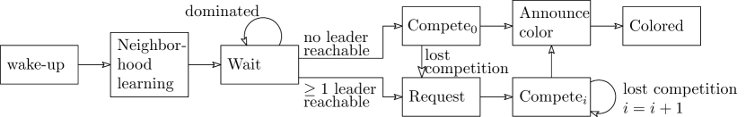
Figure 1: State diagram of the MW-coloring algorithm.

The coloring algorithm for node $v$ starts with a listening phase, which is long enough so that $v$ knows the current status of all other nodes that are awake and can reach $v$. Afterwards, if there is a leader $w$ to which bidirectional communication is possible, $v$ enters the request state, and requests a color from $w$. After $w$ answers the request by assigning a color $j$, $v$ tries to verify the assigned color $j$. If this is not successful (i.e., $v$ loses against another node competing for $j$ that reaches $v$), $v$ increases $j$ by one and retries. If $v$ is successful, it announces its success until all the nodes that can hear $v$ are informed about $v$’s status and hence know that $v$ will color itself with color $j$.

If there is no leader that can communicate bidirectionally with $v$, $v$ tries to compete for the status leader. If this is not successful, $v$ enters the request state (and proceeds as above) as there is a leader with bidirectional communication available now. Note that $v$ does not lose against leader nodes that dominate $v$ as $v$ cannot request a color from them. If $v$ is successful in becoming leader, it selects a free leader color and announces its choice so that all nodes that can be reached by $v$ are informed. After the announcement phase, the node is officially colored and will only periodically transmit its color and serve color requests as they arrive. Note that we will call the main coloring states of the algorithm (Compete, Request, Announce and Colored) the core-coloring algorithm in this section.

Our presentation of some parts of the algorithms is based on the presentation in [3]. The pseudocode for the algorithm can be found in Algorithms 1 - 6. Let $\chi(P_{v})$ in Algorithm 3 be maximal such that $\chi(P_{v})\not\in\{d_{v}(w)-\zeta_{i},\dots,d_{v}(w)+\zeta_{i}\}$ for each $w\in P_{v}$ and $\chi(P_{v})\leq 0$ and $t_{1}$ in Algorithm 6 be the number of rounds a newly colored node has to wait before serving color requests.

Algorithm 1 Distributed node coloring in non-uniform power networks for node $v$

1:[ In$(v)$, Out$(v)]=$ Neighborhood learning()

2:Let the node store each received leader color ($M_{V}^{i}(w)$ for $i\leq\Delta+1$) for $\kappa_{s}$ time slots in C${}_{\text{taken}}$

3:Listen for $(38\Gamma^{2}+3)\kappa_{s}$ time slots

4:while $c_{v}=-1$ do $\triangleright$ This is state Wait

5:     if  (In$(v)\backslash$Out$(v))\backslash$C${}_{\text{taken}}$ $=\emptyset$ then

6:         if  (In$(v)\cap$Out$(v)\cap$C${}_{\text{taken}}=\emptyset$ then

7:              Transition to Algorithm 3: Compete${}_{0}()$

8:         else

9:              Request($w$) for a $w\in$ In$(v)\cap$Out$(v)\cap$C${}_{\text{taken}}$

10:         end if

11:     else

12:         wait for $\kappa_{s}$ time slots

13:     end if

14:end while

Algorithm 2 Neighborhood-Learning() for node $v$

The neighborhood learning algorithm is a simple three-way-handshake protocol as introduced in [18]. A node $v$ starts the neighborhood learning algorithm and thus sends a learning request with its own ID with probability $p_{s}$ for $\kappa_{s}$ time slots. For each reply it receives (at most $\Delta$), $v$ itself will acknowledge the reception.

Algorithm 3 Compete_i() for node $v$

1:The algorithm is based on the presentation in [3].

2:$P_{v}=\emptyset$, $\zeta_{i}=\begin{cases}\kappa_{l}&\mbox{if }i=0\\ \kappa_{s}&\mbox{otherwise}\end{cases}$

3:$\text{Next}=\begin{cases}\text{Request}&\mbox{if }i=0\\ \text{Compete}_{i+1}&\mbox{otherwise}\end{cases}$

4:for $\kappa_{s}$ time slots do

5:     for each $w\in P_{v}$ do $d_{v}(w)=d_{v}(w)+1$

6:     if $M_{A}^{i}(w,c_{w})$ rec. then $P_{v}=P_{v}\cup\{w\}$; $d_{v}(w)=c_{w}$

7:     if $M_{C}^{i}(w)$ rec. then goto Next; leader = $w$

8:end for

9:$c_{v}=\chi(P_{v})$

10:while $true$ do

11:     $c_{v}=c_{v}+1$

12:     if $c_{v}>\kappa_{s}$ then

13:         Announce_j() for $j\begin{cases}\text{minimal}\not\in$ C$_{\text{taken}}&\mbox{if }i=0\\ i&\mbox{otherwise}\end{cases}$

14:     end if

15:     for each $w\in P_{v}$ do $d_{v}(w)=d_{v}(w)+1$

16:     transmit $M_{A}^{i}(v,c_{v})$ with probability $p_{s}$

17:     if $M_{C}^{i}(w$ rec. then goto Next; leader = $w$

18:     if $M_{A}^{i}(w,c_{w})$ rec.  then

19:         $P_{v}=P_{v}\cup\{w\}$; $d_{v}(w)=c_{w}$

20:         if $|c_{v}-c_{w}|\leq\zeta_{i}$ then $c_{v}=\chi(P_{v})$

21:     end if

22:end while

Algorithm 4 Request($w$) for node $v$

1:Transmit $M_{R}^{v}(w)$ with prob. $p_{s}$ for $\kappa_{s}$ slots to leader $w$

2:Wait for $\kappa_{s}$ rounds to receive color assignment $j$.

3:Transition to Algorithm 3 (Compete) with $i=j$

Algorithm 5 Announce_i() for node $v$

1:Transmit the $M_{C}^{i}(v)$ announcement with $p_{l}$($p_{s}$) for $\kappa_{l}$($\kappa_{s}$) slots for leader / non-leader colors

2:Wait & Transmit $M_{C}^{i}(v)$ with $p_{s}$ for $\kappa_{s}$ slots

3:Goto Algorithm 6: Colored_i()

Algorithm 6 Colored_i() for node $v$

1:count $=0$, current $=-1$, serveCount $=1$

2:while $true$ do

3:     count = count$+1$

4:     Transmit $M_{C}^{i}(v)$ with probability $p_{s}$

5:     if $M_{R}^{w}(v)$ received then $Q=Q$.add($w$)

6:     if count $>t_{1}$ and $i\leq 9\Gamma^{2}+1$ then

7:         $\triangleright$ Only for leader nodes that serve requests

8:         if count $>t_{1}+\kappa_{l}$ or current $=-1$ then

9:              count $=t_{1}$, serveCount = serveCount $+1$

10:              $j=$serveCount $\cdot 38\Gamma^{2}$.

11:              current = $Q$.first$()$ (or -1 if $Q$ empty)

12:         end if

13:         if current $\not=-1$ then

14:              Transmit $M_{S}^{\text{current}}(j)$ for $\kappa_{l}$ slots with prob. $p_{l}$, where $j$ is a free color (interval)

15:         end if

16:     end if

17:end while

In order to allow leaders faster communication, the algorithm uses two different transmission probabilities. Let the transmission probability commonly used by non-leader nodes be $p_{s}=\gamma/(2\Delta)$ and the transmission probability reserved for special leader tasks (i.e., announcement of winning a leader competition or answering color requests) $p_{l}=\gamma/(18\Gamma^{2})$.

5.2 Analysis

Let us now begin with the analysis of the algorithm, which is split in two parts. The first part shows that the transmissions conducted in the algorithm are successful with high probability. In the second part we will show that the algorithm computes a valid $\mathcal{O}(\Gamma^{2}\Delta)$ coloring, and terminates after at most $\mathcal{O}((\ell+\Delta)\Gamma^{6}\Delta\log n)$ time slots.

5.2.1 Transmissions are successful

In order to apply the bound in the interference shown in Section 3, we need to bound the sum of sending probabilities from within each transmission region.

Lemma 6.

Let $v$ be an arbitrary leader node. Then there are at most $9\Gamma^{2}$ other leader nodes in the transmission range of $v$.

Proof.

Note that leaders do not necessarily form an independent set, as an unidirectional communication link between leaders is allowed in the algorithm. Let us consider an arbitrary leader node $v$. It holds that within distance $\mkern 3.5mu\underline{\mkern-3.5mu\operatorname{R}\mkern-3.5mu}\mkern 3.5mu$ there cannot be another leader, as otherwise there would be a bidirectional communication link between two leader nodes. This is not possible as one of them would not have become leader but requested a color from the other. Thus it holds that for discs of size $\mkern 3.5mu\underline{\mkern-3.5mu\operatorname{R}\mkern-3.5mu}\mkern 3.5mu/2$ around each leader node in $v$’s neighborhood, these discs do not intersect. Hence it holds that there can be at most $\frac{(\bar{\operatorname{R}}+\mkern 3.5mu\underline{\mkern-3.5mu\operatorname{R}\mkern-3.5mu}\mkern 3.5mu/2)^{2}}{(\mkern 3.5mu\underline{\mkern-3.5mu\operatorname{R}\mkern-3.5mu}\mkern 3.5mu/2)^{2}}\leq 9\Gamma^{2}$ leader nodes in a maximal transmission range. ∎

Lemma 7.

Let leader nodes send with probability $p_{l}$ and non-leader nodes with probability $p_{s}$, then the sum of transmission probabilities from within each transmission region is upper bounded by $\gamma$.

Proof.

Let us consider an arbitrary node $v$ and sum over the transmission probabilities from within $v$’s transmission region

$$\sum_{w\in B_{v}}p_{w}\leq 9\Gamma^{2}p_{l}+\Delta p_{s}\leq\gamma$$

This holds as at most $9\Gamma^{2}$ leader nodes from each transmission region may transmit with probability $p_{l}$ due to Lemma 6, while at most $\Delta$ other nodes in $v$’s neighborhood transmit with probability at most $p_{s}$. ∎

The corollary follows from the lemma along with the argumentation for Theorem 2. It shows that the limited number of leader nodes are able to communicate to their neighbors in $\mathcal{O}(\log n)$ time slots, while non-leader nodes require $\mathcal{O}(\Delta\log n)$ time slots. Overall it implies that all transmissions in the algorithm are successful w.h.p.

Corollary 8.

A message that is transmitted with probability $p_{l}$ ($p_{s}$) for $\kappa_{l}=8c/p_{l}\log n$ ($\kappa_{s}=8c/p_{s}\log n$) time slots reaches its intended receivers w.h.p.

This shows that communication is successful with high probability even in this more general case. Combined with the algorithmic changes and the refined analysis in the full version of this paper [5], the modified MW-coloring algorithm computes a coloring with $\mathcal{O}(\Gamma^{2}\Delta)$ colors such that each color forms an independent set in $\mathcal{O}((\Delta+\ell)\Gamma^{4}\Delta\log n)$ time slots. This highlights the applicability of our method to bound the interference in networks of nodes with arbitrary transmission powers.

5.2.2 Runtime of the algorithm

In this section we consider the runtime of the distributed node coloring algorithm. We will first state the main result of this section.

Theorem 5.

After running the coloring algorithm (Algorithm 1) for at most $\mathcal{O}((\Delta+\ell)\Gamma^{4}\Delta\log n)$ time slots, all nodes are colored.

The proof follows from the lemmata stated in this section and a worst case execution of the algorithm. Let us therefore consider such a worst case. The nodes starts with executing the neighborhood learning protocol. Afterwards it will be dominated for the maximal time. Then, finally the will be able to start running the core coloring algorithm. It will therefore enter Compete₀ state, fail to win and hence enter Request state afterwards. After going through the maximum number of Compete_i states, it will finally win a competition and move (through announce) to the coloring state. Summing over the maximal runtime of the states shows the theorem.

Table 1: Runtime of the algorithm. CC stands for parts of the core coloring algorithm

State	Runtime	Proof
Neighborhood learning	$(2\Delta+1)\kappa_{s})$	Lemma 9
Wait state	$\ell\cdot$ Coloring	Lemma 10
CC: Compete0	$3\kappa_{s}+\Delta\kappa_{l}$	Lemma 11
CC: Competei	$(38\Gamma^{2}+3)\kappa_{s}$	Lemma 12
CC: Max. Competei’s	$(38^{2}\Gamma^{4}+120\Gamma^{2})\kappa_{s}$	Lemma 13
CC: Request	$(38+4)\kappa_{s}+\Delta\kappa_{l}$	Lemma 14
CC: Announce	$\leq 2\kappa_{s}$	-

In the following we prove the results stated in Table 1. In the next lemma the runtime of the initial neighborhood learning protocol bounded from above.

Lemma 9.

Let a node $v$ execute Algorithm 2. After the execution, both $v$ and its neighbors $w_{i}$ know about their communication link and whether the link is bidirectional. The algorithm finishes within $2\Delta+1\kappa_{s}$ time slots.

Proof.

As node $v$ transmits a neighborhood learning request to all its neighbors $w_{i}$, the neighbor answers within $\Delta\kappa_{s}$ slots after receiving the request (he may serve at most $\Delta-1$ other request in the meantime. If the $w_{i}$ reaches $v$, $v$ receives the message and completes the three-way-handshake by acknowledging the reception of the message to $w_{i}$, again within at most $\Delta\kappa_{s}$ slots. This holds for all neighbors. ∎

After finishing the initialization, each node needs to wait until it is no longer dominated. In the following we will argue that the core coloring algorithm needs to run at most $\mathcal{O}(\ell)$ times before all nodes are colored.

Lemma 10.

Each node $v$ that reached Line 4 of Algorithm 1 and is not dominated, will be colored after $\mathcal{O}(\Gamma^{4}\kappa_{s})$ time slots.

Proof.

The runtime of the different states of the core coloring algorithms are as depicted in Table 1. Let us now assume a node $v$ is not dominated and in the required loop. It will then start executing the core coloring algorithm. The worst case runtime of the core coloring algorithm is $\mathcal{O}(\Gamma^{4}\kappa_{s})$ time slots. This follows from the argumentation after Theorem 5. ∎

Specifically, the lemma implies that once a node reached Line 4 of Algorithm 1, it will be colored after at most $\mathcal{O}(\ell\Gamma^{4}\kappa_{s})$ time slots. This holds since initially the length of the longest directed chain of dominating nodes is $\ell$. Due to Lemma 10, the length of the longest uncolored directed path is at most $\ell-1$ after $\mathcal{O}(\Gamma^{4}\kappa_{s})$ time slots. After repeating this procedure for $\ell$ times, the length of the longest uncolored directed path is $0$ and hence there are no dominated nodes. Thus after one more execution of the core coloring algorithms all nodes are colored. Let us now consider the states of the core-coloring algorithm. We begin with the compete states for leader and non-leader nodes.

Lemma 11.

Let $v$ be a node entering the Compete₀ state. At most $3\kappa_{s}+\Delta\kappa_{l}$ slots after entering Compete₀, $v$ leaves the state.

Proof.

There are two cases. Either $v$ wins the competition and will become leader or loses and enters the request state afterwards. In both cases the initial listen stage takes $\kappa_{s}$ slots. However, as soon as $v$ transmits once (which is after at most another $\kappa_{s}$ slots), he cannot be reset anymore according to Lemma 16. Hence either $c_{v}$ reaches $\kappa_{s}$ and $v$ becomes leader or another node reaches $\kappa_{s}$ first (with sufficient time before $c_{v}$ reaches $\kappa_{s}$) and hence forces $v$ in the request state. As the counter $c_{v}$ may at worst be reset to $\Delta\kappa_{l}$, the overall runtime of state Compete₀ is $3\kappa_{l}+\Delta\kappa_{s}$. ∎

Lemma 12.

Let $v$ be a node entering the Compete_i state. At most $(38\Gamma^{2}+3)\kappa_{s}$ slots after entering Compete_i, $v$ leaves the state.

Proof.

The Lemma follows from an argumentation analog to that of Lemma 11. ∎

If a non-leader fails to verify the color $i$ it got assigned from its leader, it tries to verify $i+1$ and so on. Thus non-leader nodes may be in more than one consecutive compete states. We will now bound the number of consecutive compete states a node may be forced to visit before being able to verify a color.

Lemma 13.

A node can only be in $38\Gamma^{2}$ consecutive compete state and leaves the last compete state at most $38^{2}\Gamma^{4}+114\Gamma^{2}+6)\kappa_{s}$ slots after entering the first..

Proof.

Let us consider a node $v$ that got color $j$ assigned by its leader. It hold that the node will try to verify $j$ or a consecutive color, until it wins a competition and enters the announce state. Let us consider the number of nodes that could force $v$ to move on to the next color. By Lemma 18, this number is upper-bound by $38\Gamma^{2}$. Hence after at most $38\Gamma^{2}$ consecutive compete states all nodes that may compete with $v$ for the same color are colored and hence $v$ succeeds in the following competition round. ∎

After proving the bound in the runtime of the compete states, let us consider the request state.

Lemma 14.

A node $v$ that enters the request state leaves the request state at most $(38+4)\kappa_{s}+\Delta\kappa_{l}$ time slots afterwards.

Proof.

The node $v$ first sends it’s request in $\kappa_{s}$ slots, and subsequently will be served by its leader. As the leader may still be in the initial not-yet-serving-requests phase (see Algorithm 6), it may require up to $(38\Gamma^{2}+3)$ slots until the leader starts serving the requests. As the leader can have at most $\Delta$ request, $v$ will be served at most $\Delta\kappa_{l}$ slots later. ∎

5.2.3 Correctness of the algorithm

In order to ensure the correctness of the algorithm it remains to show that the algorithm indeed computes a valid node coloring with at most $\mathcal{O}(\Gamma^{2}\Delta)$ colors.

Theorem 6.

The coloring algorithm (Algorithm 1) computes a coloring with $\mathcal{O}(\Gamma^{2}\Delta)$ colors such that each color forms an independent set.

We will show the theorem in two steps. We will first show that indeed each color forms an independent set and afterwards bound the number colors used by the algorithm.

Proof.

Let us consider two nodes $u$ and $v$ that are colored with the same color $i$. Let us first assume there is a bidirectional communication link between $u$ and $v$. If $u$ and $v$ competed for $i$ at the same time, $u$ and $v$ cannot finish within less than $\kappa_{l}$ (or $\kappa_{s}$) time slots. Thus let us assume $v$ finished before $u$. Then, $v$ was able to announce $i$ to $u$ and force $u$ to move to another color or the request state. If $u$ and $v$ did not compete at the same time, let $v$ be the node colored earlier. Again, $v$ was able to communicate to $u$ that it is colored with $i$ and thus prevented $u$ from verifying $i$. Note that at least once $v$ reached $u$ less than $\kappa_{s}$ time slots before $u$ finishes, hence $i$ is in C${}_{\text{taken}}$ of $u$. ∎

Let us now bound the number of colors

Proof.

As $9\Gamma^{2}$ is an upper bound on the number of other leader nodes that can be in the transmission range of a leader node, this is the maximal number of colors that can be blocked when a leader node selects it’s color. Hence $9\Gamma^{2}+1$ leader colors are sufficient. The number of non-leader colors is bound by the number of requests a leader may have to serve in the worst case. This is obviously $\Delta$ as bidirectional communication is required. Due to Lemma 13 it holds that for each request at most $38\Gamma^{2}$ consecutive colors are required. After noticing that $38\Gamma^{2}$ is the first non-leader color that is assigned it holds that at most $38\Gamma^{2}(\Delta+1)$ non-leader colors are used by the algorithm. ∎

5.2.4 Asynchronous node wakeup

Let us now briefly consider the asynchronous wake-up of nodes. In order to allow nodes to start after other nodes finished the neighborhood learning protocol, we allow both algorithms to run in parallel by requiring each node to reserve every second round of “local broadcasting” for answering possible neighborhood learning requests. This requires to account twice the number of time slots for each transmission, as well as each request. This doubles the runtime of the algorithm, but enables the algorithm to cope with asynchronous node wakeup.

We assume that two nodes that currently execute the core-coloring algorithm do not have an unidirectional link. However, such an unidirectional link might be introduced due to an awaking node. To prevent this, we require nodes that are not yet colored to stop executing the core-coloring algorithm and return to the main loop of Algorithm 1 immediately if they get dominated. Note that colored leaders need to store which colors they assigned to which nodes and reuse them accordingly in order to ensure the bound on the number of colors in the previous section. Note that if a node $v$ is already colored it is not required to stop running the core coloring algorithm. However, as a node that has a unidirectional communication link to $v$ selects the same color as $v$, $v$ needs to resign from its color.

Thus if a node $v$ that is colored with color $i$ receives an announcement from node $w$ that $w$ will take color $i$, $v$ finishes serving its requests and then resigns from the color and enters the main loop of Algorithm 1. Note that $v$ cannot be in the initial phase in which it is not yet allowed to serve requests. Otherwise $w$ would have been in the core coloring algorithm at the same time as $v$ and dominated $v$. Hence $v$ could not verify the leader color $i$ (due to the listen-phase in Algorithm 1).

As we do also have to handle nodes that go to sleep asynchronously, we require the nodes to enter the main loop of the algorithm if for example a request is not answered within the time boundaries proven in Section 5.2.2.

Note that the runtime of the algorithm holds only for stable parts of the network. As nodes that wake up may force other nodes to resign, we cannot guarantee a runtime based only on the wake up time of the node itself. However, the runtime of Theorem 5 holds for $v$ after the last node that can reach $v$ or one of $v$’s neighbors directly or through a directed chain woke up. This holds as $v$ can only be forced to stop the algorithm or resign from its color by a node that reaches $v$ directly or through a directed chain. However, $v$ may expect a delay for example in the request state only if a neighbor of $v$ is forced to resign.

5.3 Maximal Independent Set

An algorithm for solving MIS can be deducted by simplifying our coloring algorithm. As nodes can either be in the MIS or not, we do only require two colors. Let 0 be to color that indicates that a node is in the MIS and 1 that it is not. As all nodes in the MIS are independent, we do not require the request state, and nodes in the MIS do not need to serve requests. Also, once a node $v$ that is executing the core-coloring algorithm receives a $M_{C}^{0}(w)$ message, $v$ can instantly transition to the Colored${}_{1}()$ algorithm. After a runtime of $\mathcal{O}((\Delta^{2}+\ell)\Gamma^{\bar{\alpha}+4}\log n)$, each node selected a color and thus either is in the MIS or not.

6 Conclussion

In this paper we have proven a bound on the interference in networks with arbitrary transmission power assignments in wireless ad hoc networks. We believe that this generic result will be of use in many algorithms designed for such networks. We have shown that local broadcasting can be transfered to the general case of arbitrary transmission powers with minor efforts due to this result. Additionally, we considered variable transmission power, which allows each node to change its transmission power in each time slot. To highlight the applicability of our results on communication in networks with arbitrary transmission power, we presented a distributed node coloring algorithm that is fully adapted to characteristics of directed communication networks such as unidirectional communication links. For future directions, we wonder whether the dependence on the neighborhood learning algorithm is required and whether the dependence on $\Gamma$ could be decreased.

Appendix A Omitted Proofs

A.1 Proof of Theorem 2

We shall prove the theorem in three steps. First, we establish that within the transmission radius of each node the transmission probability is constant. Then, we consider the the probabilistic interference that origins from the area close to the sender, and finally we sum over the probabilistic interference from all nodes in the network by exploiting that if not too many nodes transmit in any part of the network the interference from further away parts are negligible.

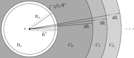
Figure 2: Sketch of proof

We are now able to proof the result using standard techniques from [7] combined with the results in Section 3.

Theorem 2.

Let the transmission probability of each node be $p=\gamma/\Delta$, and $c>1$ an arbitrary constant. A node $v$ that transmits with probability $p$ for $8c/p\log n=\mathcal{O}(\Gamma^{2}\Delta\log n)$ time slots successfully transmits to its neighbors whp.

Proof.

Let $v$ be the node that transmits for $8c/p\log n$ time slots with probability $p$. We prove the theorem by first showing that the probability of a successful local broadcast of $v$ in each round it transmits is substantial, followed by proving that at least one successful local broadcast of $v$ happens with high probability within $8c/p\log n$ time slots $v$

It is stated in Theorem 1 that the probabilistic interference from all nodes not in $\bar{\operatorname{R}}^{v}$ is upper bounded by $(\delta-1)\bar{{\operatorname{N}}}/2$. With the standard Markov inequality it follows that the probability that the interference from outside of the maximal transmission radius exceeds $(\delta-1)\bar{{\operatorname{N}}}$ with probability less than $1/2$ and thus that the SINR condition holds with probability at least $1/2$. Combining both probabilities with the transmission probability of $v$ yields a lower bound on the success of a local broadcast by $v$ in each time slot.

$$P_{\text{success}}\geq\frac{p}{8}$$

Using this probability we can bound the probability that $v$ fails in having a successful local broadcast within $8c/p\log n$ time slots.

$$P_{\text{fail}} \leq\left(1-\frac{p}{8}\right)^{8c/p\log n}=\left(1-\frac{c\log n}{8/pc\log n}\right)^{8c/p\log n}\overset{(1)}{\leq}e^{-c\log n}=\frac{1}{n^{c}},$$

where (1) follows from Fact 2. Hence within $8c/p\log n=O(\Gamma^{\bar{\alpha}+2}\Delta\log n)$ time slots, at least one of the transmissions of $v$ is successfully heard by all nodes in $B_{v}$ with high probability. ∎

A.2 Coloring

The following lemmata are required to ensure that the counters in compete states are not reset for ever, but that some nodes will be able to reach the counter limit and thus get colored.

Lemma 15.

For the counter value $c_{v}$ of a node $v$ in the compete state it holds that $c_{v}\geq-\Delta\kappa_{l}$ if $v$ is in state Compete₀, and $c_{v}\geq-(38\Gamma)\kappa_{s}$ if $v$ is in state Compete_i for $i>0$.

Proof.

The lemma follows directly from the argumentation for Lemma 5 in [3]. ∎

Lemma 16.

For a node $v$ in the compete state it holds that once he successfully transmitted a message with its counter value $c_{v}$ to its neighbors, it cannot be reset anymore.

Proof.

The lemma follows directly from the argumentation for Lemma 6 in [3]. ∎

A.2.1 Bounding the number of compete states

The following two lemmata are required to bound the number of consecutive compete states.

Lemma 17.

Let $v$ be an arbitrary node. Then at a given time slot at most $19\Gamma^{2}$ leader nodes can be within a distance of $2\bar{\operatorname{R}}$ of $v$.

Proof.

With the same argumentation as in the proof of Lemma 7, it holds that discs with radius $\mkern 3.5mu\underline{\mkern-3.5mu\operatorname{R}\mkern-3.5mu}\mkern 3.5mu/2$ around the leader nodes do not intersect, and are fully contained in a disc of radius $2\bar{\operatorname{R}}+\mkern 3.5mu\underline{\mkern-3.5mu\operatorname{R}\mkern-3.5mu}\mkern 3.5mu/2$ around $v$. Thus at most $\frac{{\operatorname{Area}}(2\bar{\operatorname{R}}+\mkern 3.5mu\underline{\mkern-3.5mu\operatorname{R}\mkern-3.5mu}\mkern 3.5mu/2)}{{\operatorname{Area}}(\mkern 3.5mu\underline{\mkern-3.5mu\operatorname{R}\mkern-3.5mu}\mkern 3.5mu/2)}\leq 19\Gamma^{2}$ nodes can be leaders within distance $2\bar{\operatorname{R}}$ around $v$. ∎

Lemma 18.

Given a network with asynchronous wake-up of nodes. Let $v$ be an active node that tries to verify the assigned color $j$. Then there are at most $38\Gamma^{2}$ nodes $u_{1},\dots,u_{c}$ that are active, capable of communicating with $v$, and that try to verify the same color $j$ as $v$.

Proof.

Let us consider a time slot $t$ such that $t$ is the first time slot in which a node $v$ competes with more than $38\Gamma^{2}$ nodes for the same non-leader color $j$. Let us denote the upper bound on the time it takes to compete for one color as $T$ for the sake of simplicity. As $t$ is the first time slot, it holds that all nodes that received a color-assignment $38\Gamma^{2}T$ time slots before $t$ or earlier must have finished competing for the considered color $j$.

Due to Lemma 17 at most $19\Gamma^{2}$ nodes can be leaders around $v$, and thus in a given period of at least $19\Gamma^{2}T$ time slots at most $19\Gamma^{2}$ nodes within distance $\bar{\operatorname{R}}$ of $v$ can get the same color assigned as $v$ (due to the listen period of $19\Gamma^{2}T$ time slots before a new leader node answers requests). Hence within the $38\Gamma^{2}T$ time slots before $t$, at most $38\Gamma^{2}$ nodes may compete for color $j$, contradicting the choice of $t$ and implying the lemma. ∎

A.3 Useful facts

Fact 1.

(proven in [10])

Given a set of probabilities $p_{1},\dots,p_{n}$ with $\forall i:p_{i}\in[0,\frac{1}{2}]$, the following inequalities hold:

$$\left(\frac{1}{4}\right)^{\sum_{k=1}^{n}p_{k}}\leq\prod_{k=1}^{n}(1-p_{k})\leq\left(\frac{1}{e}\right)^{\sum_{k=1}^{n}p_{k}}$$

Fact 2.

(for example in the mathematical background section of [14])

For all $n$, $t$, such that $n\geq 1$ and $|t|\leq n$,

$$e^{t}(1-\frac{t^{2}}{n})\leq(1+\frac{t}{n})^{n}\leq e^{t}.$$

A.4 A Worst Case Network

Figure 3: A network that requires $\Omega(n)$ time slots to allow each node one local broadcast if the broadcasting range equals the transmission range.

References

- [1] L. Barenboim and M. Elkin. Distributed Graph Coloring: Fundamentals and Recent Developments. Synthesis Lectures on Distributed Computing Theory. Morgan & Claypool Publishers, 2013.
- [2] S. Daum, S. Gilbert, F. Kuhn, and C. Newport. Broadcast in the ad hoc sinr model. In Y. Afek, editor, Distributed Computing, volume 8205 of Lecture Notes Comput. Sci., pages 358–372. Springer Berlin Heidelberg, 2013.
- [3] B. Derbel and E.-G. Talbi. Distributed Node Coloring in the SINR Model. In Proc. 30th Internat. Conf. on Distributed Computing Systems (ICDCS’10), pages 708–717. IEEE Computer Society, 2010.
- [4] F. Fuchs and D. Wagner. On Local Broadcasting Schedules and CONGEST Algorithms in the SINR Model. In Proc. 9th Internat. Workshop on Algorithmic Aspects of Wireless Sensor Networks (ALGOSENSORS’13), pages 170–184, 2013.
- [5] F. Fuchs and D. Wagner. Arbitrary transmission power in the sinr model: Local broadcasting, coloring and mis. CoRR, abs/1402.4994, 2014.
- [6] T. Fujii, T. Takahashi, T. Bandai, T. Udagawa, and T. Sasase. An efficient mac protocol in wireless ad-hoc networks with heterogeneous power nodes. In 5th Internat. Symp. Wireless Personal Multimedia Communications (WPMC’02), volume 2, pages 776–780. IEEE, 2002.
- [7] O. Goussevskaia, T. Moscibroda, and R. Wattenhofer. Local Broadcasting in the Physical Interference Model. In Proc. 5th ACM Internat. Workshop on Foundations of Mobile Computing (DialM-POMC’08), pages 35–44. ACM Press, 2008.
- [8] M. M. Halldórsson and P. Mitra. Towards Tight Bounds for Local Broadcasting. In Proc. 8th ACM Internat. Workshop on Foundations of Mobile Computing (FOMC’12). ACM Press, July 2012.
- [9] M. M. Halldórsson and P. Mitra. Wireless connectivity and capacity. In Proc. 23th Ann. ACM-SIAM Symp. Discrete Algorithms (SODA’12), SODA ’12, pages 516–526. SIAM, 2012.
- [10] T. Jurdziński and G. Stachowiak. Probabilistic algorithms for the wakeup problem in single-hop radio networks. In Algorithms and Computation, pages 535–549. Springer, 2002.
- [11] T. Kesselheim and B. Vöcking. Distributed contention resolution in wireless networks. In Proc 24th Internat. Symp. on Distributed Computing (DISC’10), pages 163–178, Berlin, Heidelberg, 2010. Springer-Verlag.
- [12] T. Moscibroda and M. Wattenhofer. Coloring Unstructured Radio Networks. J. Distr. Comp., 21(4):271–284, 2008.
- [13] T. Moscibroda and R. Wattenhofer. Coloring unstructured radio networks. In Proc 17th ACM Symp. on Parallelism in Algorithms and Architectures (SPAA’05), pages 39–48. ACM, 2005.
- [14] R. Motwani and P. Raghavan. Randomized algorithms. Chapman & Hall/CRC, 2010.
- [15] D. Peleg. Distributed Computing: A Locality-Sensitive Approach. Society for Industrial Mathematics, 2000.
- [16] N. Poojary, S. V. Krishnamurthy, and S. Dao. Medium access control in a network of ad hoc mobile nodes with heterogeneous power capabilities. In IEEE Internat. Conf. on Communications (ICC’01), volume 3, pages 872–877. IEEE, 2001.
- [17] J. Schneider and R. Wattenhofer. Coloring unstructured wireless multi-hop networks. In Proc. 28th ACM Symp. on Principles of Distributed Computing (PODC’09), pages 210–219. ACM, 2009.
- [18] R. S. Tomlinson. Selecting sequence numbers. In Proc. of 1975 ACM SIGCOMM/SIGOPS Workshop on Interprocess Communications, pages 11–23, New York, NY, USA, 1975. ACM.
- [19] G. Wang, D. Turgut, L. Bölöni, Y. Ji, and D. C. Marinescu. A mac layer protocol for wireless networks with asymmetric links. Ad Hoc Networks, 6(3):424–440, 2008.
- [20] D. Yu, Q.-S. Hua, Y. Wang, and F. C. M. Lau. An O(log n) Distributed Approximation Algorithm for Local Broadcasting in Unstructured Wireless Networks. In Proc. 8th Internat. Conf. on Distributed Computing in Sensor Systems (DCOSS’12), pages 132–139. IEEE Computer Society, 2012.
- [21] D. Yu, Y. Wang, Q.-S. Hua, and F. C. M. Lau. Distributed ( + 1) Coloring in the Physical Model. In Proc. 7th Internat. Workshop on Algorithmic Aspects of Wireless Sensor Networks (ALGOSENSORS’11), Lecture Notes Comput. Sci., pages 145–160. Springer, 2011.
- [22] D. Yu, Y. Wang, Q.-S. Hua, and F. C. M. Lau. Distributed Local Broadcasting Algorithms in the Physical Interference Model. In Proc. 7th Internat. Conf. on Distributed Computing in Sensor Systems (DCOSS’11), pages 1–8. IEEE Computer Society, 2011.
- [23] M. Zuhairi, H. Zafar, and D. Harle. On-demand routing with unidirectional link using path loss estimation technique. In Proc. Wireless Telecommunications Symposium (WTS’12), pages 1–7, 2012.