Fast matrix computations for functional additive models
Abstract
It is common in functional data analysis to look at a set of related functions: a set of learning curves, a set of brain signals, a set of spatial maps, etc. One way to express relatedness is through an additive model, whereby each individual function is assumed to be a variation around some shared mean . Gaussian processes provide an elegant way of constructing such additive models, but suffer from computational difficulties arising from the matrix operations that need to be performed. Recently Heersink & Furrer have shown that functional additive model give rise to covariance matrices that have a specific form they called quasi-Kronecker (QK), whose inverses are relatively tractable. We show that under additional assumptions the two-level additive model leads to a class of matrices we call restricted quasi-Kronecker (rQK), which enjoy many interesting properties. In particular, we formulate matrix factorisations whose complexity scales only linearly in the number of functions in latent field, an enormous improvement over the cubic scaling of naïve approaches. We describe how to leverage the properties of rQK matrices for inference in Latent Gaussian Models.
1 Introduction
One of the most frequent scenarios in functional data analysis is that one has a group of related functions (for example, learning curves, growth curves, EEG traces, etc.) and the goal is to describe what these functions have in common and how they vary (Ramsay and Silverman,, 2005; Behseta et al.,, 2005; Cheng et al.,, 2013). In that context functional additive models are very natural, and the simplest is the following two-level model:
| (1) |
where functions are individual functions (e.g. learning curves for different individuals), is a mean function and describe individual differences.
The two-level model appears on its own, or as an essential building block in more complex models, which may include several hierarchical levels (as in functional ANOVA, Ramsay and Silverman,, 2005; Kaufman and Sain,, 2009; Sain et al.,, 2011), time shifts (Cheng et al.,, 2013; Kneip and Ramsay,, 2008; Telesca and Inoue,, 2008), or non-Gaussian observations (Behseta et al.,, 2005). Functional PCA (Ramsay and Silverman,, 2005), which seeks to characterise the distribution of the difference functions , is a closely related variant . In a Bayesian framework the two-level model can be expressed as a particular kind of Gaussian process prior (Kaufman and Sain,, 2009). The goal of this paper is to show that the covariance matrices that arise in the two-level model have a form that lends itself to very efficient computation. We call these matrices restricted quasi-Kronecker, after Heersink and Furrer, (2011).
The paper is structured as follows. We first give some background material on Gaussian processes and latent Gaussian models (Rue et al.,, 2009), and describe the particular covariance matrices that obtain in functional additive models. These matrices are quasi-Kronecker (QK) or restricted quasi-Kronecker (rQK), and in the next section we prove some theoretical results that follow from the block-rotated form of rQK matrices. In particular, rQK matrices have very efficient factorisations, and we detail a range of useful computations based on these factorisations. In the following section we apply our results to Gaussian data (joint smoothing), and show that marginal likelihoods and their derivatives are highly tractable. The other application we highlight concerns the modelling of spike trains, which leads to a latent Gaussian model with Poisson likelihood. We show that the Hessian matrices of the log-posterior in the two-level model are quasi-Kronecker, which makes the Laplace approximation and its derivative tractable. This leads to efficient approximate inference methods for large-scale functional additive models.
1.1 Notation
The Kronecker product of and is denoted , the all-one vector of length or if obvious from the context. Throughout is used for the number of individual functions in the functional additive model, and for the number of grid points.
In what follows we will use the following two properties of the Kronecker product and vec operators (Petersen and Pedersen,, 2012):
| (2) |
for compatible matrices, and
| (3) |
where the operator stacks the columns of vertically.
1.2 Gaussian process and latent Gaussian models
We give here a brief description of Gaussian processes (GPs), a much more detailed treatment is available in Rasmussen and Williams, (2005). A GP with mean 0 and covariance function is a distribution on the space of functions of some input space into , such that for every set of sampling points , the sampled values follow a multivariate Gaussian distribution
As a shorthand for the above, we will use the notation in what follows. The covariance function usually expresses the idea that we expect the values of at and to be close if and are themselves close. Often, covariance functions only depend on the distance between two points, so that , with some distance function (usually Euclidean).
In most actual cases the covariance function is not known and involves two or more hyperparameters, which we will call . In machine learning the squared-exponential covariance function is especially popular:
| (4) |
where is a (log) length-scale parameter and controls the marginal variance of the process. For reasons of numerical stability we prefer to use a Matern 5/2 covariance function, which generates rougher functions but leads to covariance matrices that are better behaved. The Matern 5/2 covariance function has the following form:
| (5) | |||||
given in Rasmussen and Williams, (2005), page 85. The parameters and play similar roles in this formulation, controlling length-scale and marginal variance.
Gaussian processes can be used to formulate priors for Latent Gaussian Models (Rue et al.,, 2009). The term “Latent Gaussian Model” describes a very large class of statistical models, one that encompasses for example all Generalised Linear Models (with Gaussian priors on the coefficients), Generalised Mixed Models, and Generalised Additive Models. The two main components are (a) a latent Gaussian field, , with prior and (b) independently distributed data , which depend on the corresponding value of the latent field. In regression models is Gaussian, but other common distributions include a logit model (for binary ) and exponential-Poisson (as in section 3.2). The results we give here apply to all Latent Gaussian Models where the latent field has the structure of a two-level functional additive model, which we detail next.
1.3 Quasi-Kronecker structures in functional additive models
In a Gaussian process context the two-level functional additive model translates into the following model:
| (6) |
where individual ’s are conditionally independent given (they are however marginally dependent).
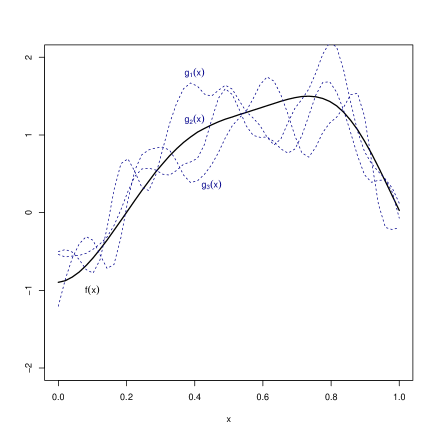
Fig. 1 gives an example of a draw from such a model. Eq. 6 expresses the model as a prior over functions, but if we have a set of sampling locations the Gaussian process assumption implies a multivariate Gaussian model for the latent field at the sample locations. We assume throughout that there are observations, corresponding to realisations of a latent process observed on a grid of size , with grid points . The grid may be irregular (i.e. needs not equal a constant), but we need the grid to be constant over individual functions, since otherwise the covariance matrix does not have the requisite structure. Denote by the vector of sampled values from : . The latent field is formed of the concatenation of , and we may think of it either as a matrix or a single vector . Following the LGM framework, we assume that the data are (possibly non-linear, non-Gaussian) observations based on the latent values, so that .
Under a particular grid, sampled values from the mean function have distribution , and has conditional distribution . Draws from the latent field can therefore be obtained by the following transformation:
| (15) | |||||
| (20) |
where and . We can use eq. 20 to find the marginal distribution of (unconditional on ). Using standard properties of Gaussian random variables we find:
| (25) | |||||
| (30) |
is a dense matrix, whose dimensions () would seem to preclude direct inference, since the costs of factorising such a matrix would be too high with numbers as low as 100 grid points and 20 observed functions. Heersink and Furrer, (2011) have shown that the matrix inverse of is actually surprising tractable, and in the following section we summarise and extend their results.
2 Some properties of restricted quasi-Kronecker matrices
Quasi-Kronecker (QK) matrices are introduced in Heersink and Furrer, (2011) and have the following form:
| (31) |
We focus mostly on the restricted case (rQK), i.e. matrices of the form
| (32) |
which arise in the functional additive model described just above (eq. 30).
QK and especially rQK matrices have a number of properties that make them much more tractable than dense, unstructured matrices of the same size.
2.1 The general (unrestricted) case
The cost of matrix-vector products with QK matrices is , as compared to in the general case. This follows directly from the definition (eq. 31), as we need only perform operations of complexity .
Heersink and Furrer, (2011) showed that the inverse and pseudo-inverse of QK matrices is also tractable. For the inverse the following formula applies:
| (33) | |||||
where . The result can be proved using the Sherman-Woodbury-Morrison formula, by writing , which follows from eq. (2). It implies that a QK matrix can be inverted in operations, as opposed to in the general case. A similar formula holds for the determinant:
| (34) |
2.2 The restricted case
rQK matrices have some additional properties not enjoyed by general QK matrices. For example, the product of two rQK matrices is another rQK matrix:
| (35) |
We use this property below to compute the gradient of the marginal likelihood in Gaussian models (section 3.1.1). In addition, several other properties follow from the block-rotated form of rQK matrices: for example, the inverse of a rQK matrix is another rQK matrix, and the eigenvalue decomposition has a very structure. We prove these results next.
2.3 Block-rotated form of rQK matrices
In this section we first establish that rQK matrices can be block-rotated into a block-diagonal form. From this result the eigendecomposition follows immediately, and so does a Cholesky-based square root. These decompositions need not be formed explicitly, and we will see that their cost scales as in storage and in time. The latter is linear in , compared to cubic for naïve algorithms.
We begin by defining block rotations, which are straightforward extensions of block permutations. A block permutation can be written using the Kronecker product of a permutation matrix and the identity matrix. Applied to a matrix , will permute blocks of size . Block rotations are defined in a similar way, through the Kronecker product of a rotation matrix and the identity matrix. A block rotation matrix is an orthogonal matrix, since:
where the second line follows from eq. (2).
Our main result is the following:
Theorem 1.
There exists an orthogonal matrix such that for all matrices , the matrix can be expressed as:
Since is an orthogonal matrix, and the inner matrix is block-diagonal, the inverse, eigendecomposition, and a Cholesky-based square root of all follow easily.
Proof.
We use the following ansatz: the matrix
is an orthogonal matrix whose first row is a scaled version of the
all-ones vector
and is chosen such that , so that the rows of L will be orthogonal to , and . Note that L is not unique, but a matrix that verifies the condition can always be found by the Gram-Schmidt process (Golub and Van Loan,, 1996) (although we will see below that a better option is available).
As noted above . We left-multiply by and right-multiply by :
| (39) | |||||
Left-multiplying by and right-multiplying by completes the proof. ∎
2.4 Inverse, factorised form, and eigenvalue decomposition
A number of interesting properties follow directly from the block-rotated form given by Theorem 1.
Corollary 2.
The inverse of an rQK matrix is also an rQK matrix. Specifically,
Proof.
This result can also be derived from the Furrer-Heersink formula (eq. 33) but follows naturally from Theorem 1. Assuming that and have full rank, then the inverse of exists and equals:
For to be an rQK matrix we need to find matrices and such that , and . This implies
which requires the existence of and , both conditions being verified if is invertible. ∎
An important consequence of this result is that Hessian matrices in latent Gaussian models with prior covariance turn out to be quasi-Kronecker (section 3.2), so that Laplace approximations can be computed in time.
Corollary 3.
The eigenvalue decomposition of is given by
where is as in theorem 1, and .
Proof.
Since is block-diagonal its eigendecomposition into is straightforward. The matrix is orthogonal: , and since with diagonal we have its eigenvalue decomposition.∎
Corollary 4.
A set of square root factorisations of is given by , with
where and .
This corollary is an entirely straightforward consequence of the theorem, but note that has special form, as the product of a block-diagonal matrix and a block-permutation matrix. In the next section we outline an algorithm that takes advantage of these properties to compute the factorisation with initial cost and further cost per MVP.
2.5 A fast algorithm for square roots of
Our fast algorithm is based on Corollary 4. Given a matrix square root , the typical operations used in statistical computation are the following:
-
•
Correlating transform: given the vector is distributed according to . The correlating transform (MVP with ) takes a IID vector and gives it the right correlation structure.
-
•
“Whitening” transform: given the vector is distributed according to . This is the inverse operation of the correlating transform and produces white noise from a correlated vector.
-
•
Evaluation of . This can be done using the whitening transform but in addition the log-determinant of is needed. We give a formula below.
Our algorithm is based on the square roots and , which can be obtained from the Cholesky or eigendecompositions. In most cases the Cholesky version is faster but the eigendecomposition has advantages in certain contexts. We outline a generic algorithm here, the only practical difference being in solving the linear systems and , which should be done via forward or back substitution if and are Cholesky factors (Golub and Van Loan,, 1996).
2.5.1 Computing the correlating and whitening transforms
Corrolary 4 tells us that the square root of , equals:
| (40) |
We first show how to compute the correlating transform. Let . Using eq. 3, we can rewrite as:
Computing the correlating transform entails MVP products with the square roots ( in the general case) and MVP products with . The latter products can be done in time, as we show below, meaning that the whole operation has total cost .
The whitening transform can be computed in a similar way:
| (43) |
so that for
and since matrix solves of the form and have cost for Cholesky or eigenfactors, the entire operation has the same cost as the correlating transform ().
2.5.2 Fast rotations
The whitening and correlating transforms above involve MVPs with a orthogonal matrix , where is such that is orthonormal. Construction of via the Gram-Schmidt process would have initial cost and MVPs with . There is however a particular choice for that brings these costs down to and :
Proposition 5.
The matrix , with and is an orthonormal basis for the set of zero-mean vectors .
The proof can be found in Appendix 5.1. With this choice of the matrix equals
| (46) |
and it is easy to check that , , and that in addition , so that . Due to the specific structure, a single MVP with has cost (which is the cost of multiplying the entries by , by and computing the sum).
2.5.3 Computing Gaussian densities and the determinant
In applications we will need to compute Gaussian densities of the following form: given
| (47) | |||||
where is obtained via whitening. In addition, the log-determinant of is needed. Similar matrices have the same determinant, so that . Further, for block-diagonal matrices, , which together with Theorem 1 implies that
| (48) |
These two log-determinants can be computed at cost from the Cholesky or eigendecompositions of and , which are needed anyway for the computation of the square root of .
2.5.4 Summary
The cost of computing matrix square roots for quasi-Kronecker matrices is dominated by the initial cost of computing two decompositions. The resulting factors have storage cost and no further storage is required. Further operations (whitening, correlating, computing the determinant) come at much lower cost ( for whitening and correlating, for the determinant).
3 Applications
We first describe how to use our techniques in the linear-Gaussian setting. Under the assumption of Gaussian observations the marginal likelihood of the hyperparameters can be computed efficiently, and we show in addition how to compute the gradient of the marginal likelihood in cost. The resulting algorithm scales very well with .
When the observations are not Gaussian, the marginal likelihood is unavailable in closed form. There are many ways to implement inference in this case, including variational inference (Opper and Archambeau,, 2008), nested Laplace approximations (Rue et al.,, 2009), expectation propagation (Minka,, 2001), various form of Markov Chain Monte Carlo (Neal,, 1997; Rue and Held,, 2005; Murray et al.,, 2010), or some combination of methods. We study in detail an example from neuroscience, smoothing of repeated spike train data, where the observations are Poisson distributed. We use a simple Laplace approximation, but our methods can be applied in a similar way to more sophisticated approximate inference or for MCMC sampling.
As stated in the introduction, we assume throughout that there are observations, corresponding to realisations of a latent process observed on a grid of size , with grid points . The grid may be irregular but it is essential that it be constant across realisations, otherwise the covariance matrix does not have the requisite form. The observations may be represented as a matrix , or equivalently as a vector .
3.1 Gaussian observations
In the Gaussian case the conditional distribution of the observations is assumed to be iid, with . To simplify the notation we will sometimes absorb the noise variance into the hyperparameters .
Depending on the scenario the goal of the analysis varies, and we
might seek to estimate the latent functions
, the latent mean
function , or to make predictions for an unobserved
function , etc. How we treat the hyperparameters
may vary as well. In a “mixed modelling” spirit we might just
want to compute their maximum likelihood estimate, or instead we may
want to perform a full Bayesian analysis and produce samples from
the posterior over hyperparameters, .
In all of these cases the main quantities of interest are:
-
1.
The (log-) marginal likelihood and optionally its derivatives with respect to the hyperparameters
-
2.
The conditional regressions and
Most of the other quantities are simply variants of the above and we will not go explicitly through all the calculations.
3.1.1 Computing the marginal likelihood and its derivatives
The marginal likelihood can be computed easily by noting that , with , so that the marginal distribution of is
and that if has rQK structure, so does . Specifically, , and we may use formula (47) directly to compute .
For maximum likelihood estimation of the hyperparameters (and for Hamiltonian Monte Carlo) it is useful to compute the gradient of with respect to the hyperparameters. To simplify notation we momentarily absorb the noise variance into the hyperparameters and note the covariance matrix of
An expression for the derivative with respect to a single hyperparameter is given by Rasmussen and Williams, (2005) (eq. 5.9):
| (49) |
It is straightforward to verify that if is rQK, so is its derivative , which implies that is also a rQK matrix (see section 2.3). Using that property along with theorem 1, some further algebra shows:
| (50) |
Computing can be done using the fast matrix square root, and is a rQK matrix, so that the dot product in eq. 49 is tractable as well (with complexity ). Given that factorisations of and are needed to compute the marginal likelihood anyway, the extra cost in computing derivatives is relatively small (the factorisations have cost , the rest is ).
3.1.2 Conditional regressions
The conditional regressions are given by the posterior distributions and . Both distributions are Gaussian, and their mean and covariance can be found through the usual Gaussian conditioning formulas:
which involves computations, and:
where is rQK and hence all computations are also . Simultaneous confidence bands can be obtained from the diagonal elements of and .
3.1.3 Fast updates
“Fast” hyperparameter updates are often available in Gaussian process models (Neal,, 2011), in the sense that one may quickly recompute the marginal likelihood from the current value . Usually a fast update means being able to skip a factorisation, and this may be done for rQK matrices as well. For example, the matrices , and (with ) all have the same eigenvectors, which means one can update certain hyperparameters without the need to recompute the square root of from scratch. Although this strategy may result in speed-ups, it requires painstaking implementation and we have not explored it further (we note however that fast updates are also linked to fast gradient computations, since eq. 49 often simplifies). It may be worthwhile when used in combination with Neal’s (2011) strategy of separating fast and slow variables.
3.1.4 Results
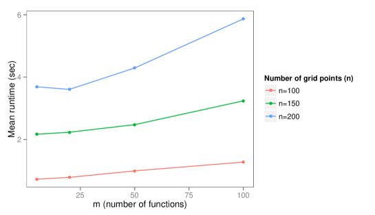
Specialised vs. generic factorisation methods
We first checked that implementing our specialised matrix factorisations is indeed worth the trouble (for reasonable problem sizes). Generic matrix factorisation techniques have been greatly optimised over the years and are often faster than an inefficient implementation of a specialised routine.
We implemented our matrix factorisation formulae in R and measured computing times for Gaussian densities . The non-specialised routine needs to first form the matrix explicitly, and uses Cholesky factorisation to evaluate the density. Our specialised implementation comes under two variants, one based on Cholesky factors, and the other based on eigendecompositions, as explained in section 2.5. The algorithms were implemented in R and all benchmarks were executed on a standard desktop PC running R 3.0.1 under Ubuntu.
Figure 2 and 3 summarise the results. We varied , the number of functions, for different values of , the grid size. General-purpose factorisation scales with , compared to our method, which scales with . What we expect, and what Fig. X verifies, is that our method should scale much better with , as indeed it does: it is faster for all but the smallest problem sizes (e.g. with and our method is not worth the bother). With we do better even with as low as 2. What the results also underscore is the relative inefficiency of eigenvalue decompositions, relative to Cholesky factorisations. The eigenvalue decomposition remains of interest for regular grids, since in this case the Fourier decomposition can be used to factorise the covariance matrix in operations (Paciorek,, 2007), or if iterative methods are used in order to get an approximate factorisation (Saad,, 2003).
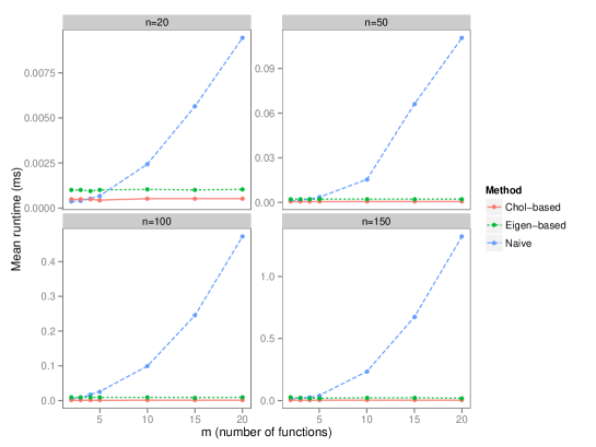
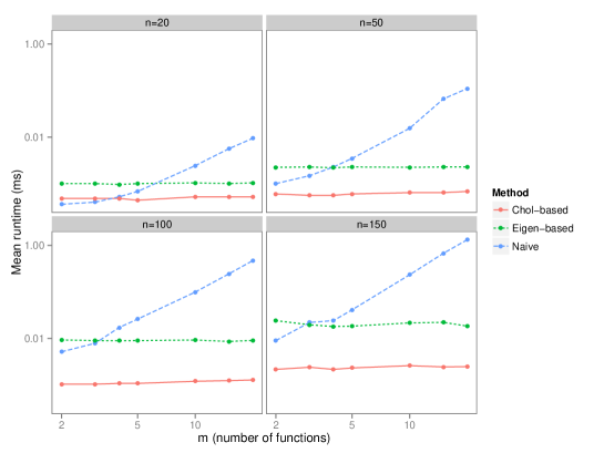
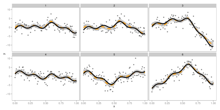
Illustration in a joint smoothing problem
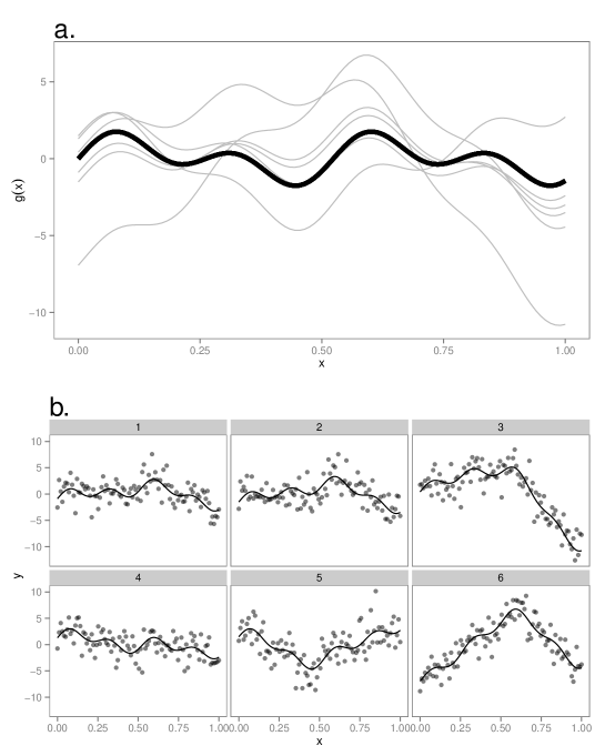
We illustrate the application of our method in a joint smoothing problem. We generated data according to the following model:
meaning that the individual functions were smooth perturbations around a fixed mean function , as shown on Fig. 4.
We use a regular grid of points .
We fitted a generic additive Gaussian process model, specifically:
The covariance functions and are Matern covariance functions, with fixed smoothness parameter . The hyperparameters to estimate are the two length-scale parameters, the two Matern variance parameters, and the noise variance . We note the vector of hyperparameters. The most straightforward estimation strategy is to maximise (maximum likelihood, ML), or alternatively (maximum a posteriori, MAP). MCMC can naturally also be used to sample from , and we compared both methods.
For MAP/ML we found that a quasi-Newton method (limited memory BFGS, Liu and Nocedal,, 1989) works very well (we used the fast analytical gradient described above), converging typically in ~ 30 iterations. The standard Gaussian approximation of at the mode can be computed by finite differences using the analytical gradient. For MCMC we used standard Metropolis-Hastings, with a proposal distribution corresponding to the Gaussian approximation of the posterior. When the data are informative enough the posterior is well-behaved and no further tuning is necessary, but problems can arise if e.g. the noise is very high and there are few measurements.
MAP inference is extremely fast (see fig. 7), and remains tractable with extremely large datasets: with a grid size of and latent functions, MAP inference takes a little over two minutes on our machine. MCMC is an order of magnitude slower but still rather tractable (it is likely that large speed-ups could be obtained using a modern Hamiltonian Monte Carlo method). Below we compare the results of MCMC and MAP inference for the data shown on fig. X.
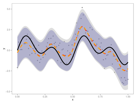
Given a MAP estimate of the hyperparameters, inference for and the ’s proceeds using the conditional posteriors and . This tends to underestimate the uncertainty in the latent processes, but the underestimation is not dramatic in this example. The simultaneous confidence bands for MAP and full MCMC inference are compared on fig. 6 (appendix 5.3 explains how the confidence bands were estimated).
3.2 Non-Gaussian observations: application to spike count data
In this section we show how to apply our technique to LGMs with non-Gaussian likelihoods, using an example where the data are Poisson counts. The Poisson LGM is one of the most popular kinds, especially in spatial statistics applications (Illian et al.,, 2008; Barthelmé et al.,, 2013). Here we focus on a application to neuroscience, specifically spike count data.
Neurons communicate by sending electrical signals (action potentials, also called spikes) to one another. Each spike is a discrete event, and the occurrence of spikes may be recorded by placing an electrode in the vicinity of a cell. Neurons respond to stimuli by modulating how much they spike. An excited neuron increases its spike rate, an inhibited neuron decreases it. In experiments where spikes are recorded a typical task is to determine how the spike rate changes over time in response to a stimulus.
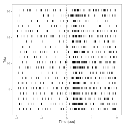
We use data provided by Pouzat and Chaffiol, (2009), which consist in external recordings of a cell in the antennal lobe of a locust, an area that responds to olfactory stimulation. Part of the data is shown on Fig. 8. The animal was stimulated by an odorant (terpineol), causing a change in the spike rate of the cell. Stimulation was repeated over the course of 20 successive trials. We look at spiking activity occurring between -2 and +2 sec. relative to stimulus onset.
The data are spike counts: we simply count the number of spikes that occurred in a given time bin. Neurons are noisy , and statistical models for spike trains are generally variations on the Poisson model , which assumes that the spike count at time follows a Poisson distribution with rate (Paninski et al.,, 2007). The goal is to infer the underlying rate , which may vary spontaneously, drift from one trial to the next, and change in response to the stimulus.
We set up the following hierarchical model:
where is the time bin and is the expected spike count in the -th bin on the -th trial.
3.3 Computing the Laplace approximation
Contrary to the Gaussian case, for generic LGMs the posterior marginals over the hyperparameters () cannot be easily computed. The Laplace approximation usually gives sensible results (Rue et al.,, 2009), although Expectation Propagation provides a superior if more expensive alternative (Nickisch and Rasmussen,, 2008).
The Laplace approximation is given by:
| (51) |
where
| (52) |
is the unnormalised log-posterior evaluated at its conditional mode , and is the Hessian of with respect to x evaluated at .
We therefore need to (a) find the conditional mode for a given value of and (b) compute the log-determinant of the Hessian at the mode. The latter is possible because the Hessian turns out to be a QK matrix, and therefore its determinant can be computed in using equation 34.
Proposition 6.
In LGMs the Hessian matrix of the log-posterior over the latent field is a quasi-Kronecker matrix.
Proof.
The second derivative of (eq. 52) with respect to is given by:
where the Hessian of the log-likelihood is diagonal (since each depends only on ) and is rQK by Corrolary 2. The sum of an rQK and a diagonal matrix is a QK matrix. ∎
However, before we can do anything with the Hessian at the mode, we need to find the mode. Proposition 6 implies that one may use Newton’s method (Nocedal and Wright,, 2006) to do so, since can be computed using equation 33. However, at each Newton step we need to solve linear systems of size , making it relatively expensive. We found that quasi-Newton methods (Nocedal and Wright,, 2006), which do not use the exact Hessian, may be more efficient provided that one chooses a smart parametrisation.
Contrary to Newton’s method, which is invariant to linear transformations of the parameters, the performance of quasi-Newton methods depends partly on the conditioning of the Hessian. It is therefore worthwhile finding a transformation so that is well-scaled. One option is to use the whitened parametrisation, i.e. (eq. 43), in which case
| (53) |
Since one of the problems with Gaussian process priors is that can have very poor conditioning, we might hope that the above transformation would help. We found that it does, but what is generally even more effective is to take into account the diagonal values of as well (preconditioning the problem). Further discussion of the issue can be found in Appendix 5.4. The Quasi-Newton method we use is limited memory BFGS in the standard R implementation (optim).
3.4 Maximising the Laplace approximation
Once we have a way of approximating , similar strategies apply in the general LGM case as do in the linear-Gaussian case. We may just require an approximate MAP estimate, or we may wish to approximately integrate out the uncertainty in using INLA (Rue et al.,, 2009) or exact MCMC in a pseudo-marginal sampler (Filippone and Girolami,, 2013). In any case the first step is to find the maximum of the Laplace approximation . Most optimisation methods will work, but it helps if the gradient can be computed. It turns out that this is possible albeit rather more expensive than in the Gaussian case, and the derivation is given in Appendix 5.2.
3.5 Results
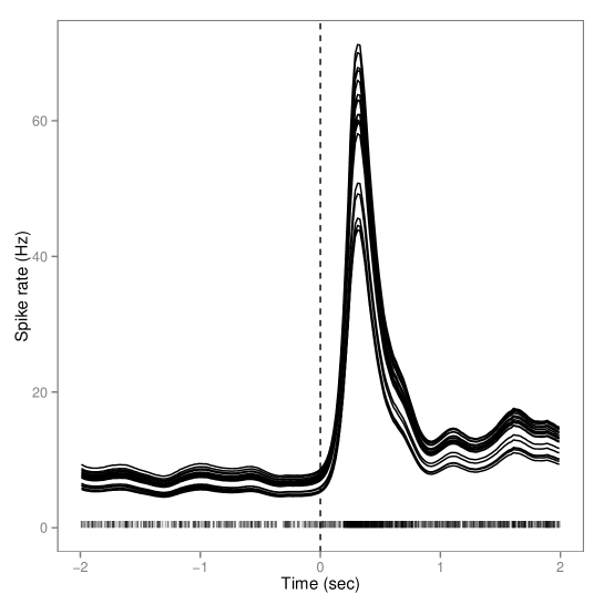
We first used the same point process models as in section 3.1 (Matern 5/2 for both and , with four hyperparameters). We used time bins of 2ms, giving a total of 200 time bins per spike train and 4,000 latent variables in total. We implemented the complete algorithm in R, and maximising the Laplace approximation takes a very reasonable 40 sec. The fitted intensity functions are shown in fig. 9. There is a sharp increase in rate following stimulus onset, but little variability across trials. Stationary Gaussian processes such as the Matern process are not very well adapted to the estimation of functions that jump about a lot, and we feared that the ripples visible in the fits (e.g. prior to stimulus onset) could be artefactual. In other words, in order not to oversmooth around the jump, the model undersmooths in other regions.
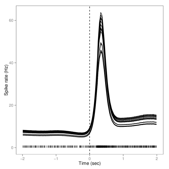
As an alternative, we formulated a model that allows nonstationarity in the mean function , assuming:
where and are two independent Matern processes, and is a mask that limits the effect of to the time around stimulus onset. The net effect is that extra variability is allowed around the time of the jump (see Bornn et al.,, 2012 for a more sophisticated approach to nonstationarity). We set and by eye. Adding hyperparameters for brings the total number of hyperparameters to 6, and fitting the nonstationary model takes about 2 minutes on our machine. The results, shown on fig. 10, indicate that pre-onset ripples are indeed most likely artefactual.
4 Conclusion
We have shown how restricted quasi-Kronecker matrices can be block rotated and factorised, and how this enables efficient inference in the two-level functional additive model. A similar closed-form factorisation for generic quasi-Kronecker matrices eludes us despite repeated attempts. That would certainly make an interesting topic for future work although perhaps not our own.
Although the algorithms we describe here scale very well with the number of functions in the dataset, they do not scale very well with grid size - the dreaded remains. For regular grids circulant embeddings (Fourier) approaches can be used (Paciorek,, 2007), although unfortunately the Laplace approximation becomes hard to compute in that setting. Iterative solvers (Saad,, 2003; Stein et al.,, 2013) could overcome the problem, but we leave that for future research.
Quasi-Kronecker and restricted quasi-Kronecker matrices display a number of appealing properties, and should probably join their block-diagonal, circulant, and Toeplitz peers among the set of computation-friendly positive definite matrices.
5 Appendix
5.1 An orthogonal basis for zero-mean vectors
We prove below proposition 5, which we restate:
Proposition.
The matrix , with and is an orthonormal basis for the set of zero-mean vectors .
Proof.
For to be an orthogonal basis for , all that is required is that for all and that . To lighten the notation, define . The first condition requires
| (54) |
and the second condition
implying that
| (55) |
This is a 2nd order polynomial in , and it has real roots if:
which is true since is non-negative.
Solving the quadratic equations yields and substituting into 54 yields .
We can therefore always find values such that is an orthogonal basis for the linear subset of zero-mean vectors. Moreover, we can show that the columns of N have unit norm:
where the last line is from 55. The result implies that we can compute an orthonormal basis for such that matrix-vector products with are . ∎
5.2 Derivative of the Laplace approximation
Using the implicit function theorem an analytical expression for the gradient of the Laplace approximation can be found (see Rasmussen and Williams,, 2005, for a similar derivation). The Laplace approximation is given by:
| (56) |
where
| (57) |
is the unnormalised log-posterior evaluated at its conditional mode , and is the Hessian of with respect to x evaluated at . Since is a maximum it satisfies the gradient equation:
Assuming that is twice-differentiable and concave in , we can define an implicit function such that for all , with derivative
| (58) | |||||
To simplify the notation we will note the matrix . Note that the same matrix appears in the gradient of the Gaussian likelihood with respect to the hyperparameters (eq. 49). To compute the gradient of , we need the derivatives of with respect to:
where the first part is 0 since the gradient of is 0 at , and
This is the gradient of a log-Gaussian density, and we can therefore reuse formula 49 for that part.
The gradient of is also needed and is sadly more troublesome. A formula for the derivative of the log-det function is given in Petersen and Pedersen, (2012):
| (59) |
The Hessian at the mode is the sum of the Hessian of (which depends on through the implicit dependency of on ), and the Hessian of , which equals the inverse covariance matrix . Some additional algebra yields:
| (60) | |||||
| (61) |
where we have assumed that the Hessian of the log-likelihood is diagonal. Accordingly is quasi-Kronecker, and so is (since it equals the sum of a rQK matrix and a diagonal perturbation ). Computing the trace in eq. (59) is therefore tractable if slightly painful, and can be done by plugging in eq. 33 and summing the diagonal elements.
5.3 Computing simultaneous confidence bands
In this section we outline a simple method for obtaining a Rao-Blackwellised confidence band from posterior samples of . A simultaneous confidence band around a latent function is a vector function , such that, for all :
In latent Gaussian models the posterior over latent functions is a mixture over conditional posteriors:
| (62) |
5.4 Preconditioning for quasi-Newton optimisation
In the whitened parametrisation the Hessian matrix has the following form (eq 53)
Although the whitened parametrisation gives ideal conditioning for the prior term, the conditioning with respect to the likelihood term () may be degraded. Preconditioning the problem can help tremendously: given a guess , one precomputes the diagonal values of and uses as a preconditioner. To compute the following identity is useful:
where is the element-wise product. In LGMs is diagonal and so:
| (63) |
We inject 43 into the above and some rather tedious algebra shows that can be computed in the following way. Form the matrix by stacking successive subsets of length from . Rotate using the matrix (section 2.5.2) to form another matrix:
then compute from:
where we have used Matlab notation subsets of columns of , and and are as in Corrolary 4.
Acknowledgements
The author wishes to thank Reinhard Furrer for pointing him to Heersink and Furrer, (2011), and Alexandre Pouget for support.
References
- Barthelmé et al., (2013) Barthelmé, S., Trukenbrod, H., Engbert, R., and Wichmann, F. (2013). Modeling fixation locations using spatial point processes. Journal of vision, 13(12).
- Behseta et al., (2005) Behseta, S., Kass, R. E., and Wallstrom, G. L. (2005). Hierarchical models for assessing variability among functions. Biometrika, 92(2):419–434.
- Bornn et al., (2012) Bornn, L., Shaddick, G., and Zidek, J. V. (2012). Modeling Nonstationary Processes Through Dimension Expansion. Journal of the American Statistical Association, 107(497):281–289.
- Cheng et al., (2013) Cheng, W., Dryden, I. L., and Huang, X. (2013). Bayesian registration of functions and curves.
- Filippone and Girolami, (2013) Filippone, M. and Girolami, M. (2013). Exact-Approximate bayesian inference for gaussian processes.
- Golub and Van Loan, (1996) Golub, G. H. and Van Loan, C. F. (1996). Matrix Computations (3rd Edition). Johns Hopkins University Press, 3rd edition.
- Heersink and Furrer, (2011) Heersink, D. K. and Furrer, R. (2011). On moore-penrose inverses of quasi-kronecker structured matrices. Linear Algebra and its Applications.
- Illian et al., (2008) Illian, J., Penttinen, A., Stoyan, H., and Stoyan, D. (2008). Statistical Analysis and Modelling of Spatial Point Patterns (Statistics in Practice). Wiley-Interscience, 1 edition.
- Kaufman and Sain, (2009) Kaufman, C. and Sain, S. (2009). Bayesian functional ANOVA modeling using Gaussian process prior distributions. Bayesian Analysis, 5:123–150.
- Kneip and Ramsay, (2008) Kneip, A. and Ramsay, J. O. (2008). Combining Registration and Fitting for Functional Models. Journal of the American Statistical Association, 103(483):1155–1165.
- Liu and Nocedal, (1989) Liu, D. and Nocedal, J. (1989). On the limited memory BFGS method for large scale optimization. Mathematical Programming, 45(1-3):503–528.
- Minka, (2001) Minka, T. P. (2001). Expectation propagation for approximate bayesian inference. In UAI ’01: Proceedings of the 17th Conference in Uncertainty in Artificial Intelligence, pages 362–369, San Francisco, CA, USA. Morgan Kaufmann Publishers Inc.
- Murray et al., (2010) Murray, I., Adams, R. P., and MacKay, D. J. (2010). Elliptical slice sampling. JMLR: W&CP, 9:541–548.
- Neal, (1997) Neal, R. M. (1997). Monte Carlo Implementation of Gaussian Process Models for Bayesian Regression and Classification.
- Neal, (2011) Neal, R. M. (2011). MCMC using ensembles of states for problems with fast and slow variables such as gaussian process regression.
- Nickisch and Rasmussen, (2008) Nickisch, H. and Rasmussen, C. E. (2008). Approximations for Binary Gaussian Process Classification. Journal of Machine Learning Research, 9:2035–2078.
- Nocedal and Wright, (2006) Nocedal, J. and Wright, S. (2006). Numerical Optimization (Springer Series in Operations Research and Financial Engineering). Springer, 2nd edition.
- Opper and Archambeau, (2008) Opper, M. and Archambeau, C. (2008). The variational gaussian approximation revisited. Neural Computation, 21(3):786–792.
- Paciorek, (2007) Paciorek, C. J. (2007). Bayesian Smoothing with Gaussian Processes Using Fourier Basis Functions in the spectralGP Package. Journal of statistical software, 19(2).
- Paninski et al., (2007) Paninski, L., Pillow, J., and Lewi, J. (2007). Statistical models for neural encoding, decoding, and optimal stimulus design. Progress in brain research, 165:493–507.
- Petersen and Pedersen, (2012) Petersen, K. B. and Pedersen, M. S. (2012). The matrix cookbook. Version 20121115.
- Pouzat and Chaffiol, (2009) Pouzat, C. and Chaffiol, A. (2009). Automatic spike train analysis and report generation. an implementation with r, R2HTML and STAR. Journal of Neuroscience Methods, 181(1):119–144.
- Ramsay and Silverman, (2005) Ramsay, J. and Silverman, B. W. (2005). Functional Data Analysis (Springer Series in Statistics). Springer, 2nd edition.
- Rasmussen and Williams, (2005) Rasmussen, C. E. and Williams, C. K. I. (2005). Gaussian Processes for Machine Learning (Adaptive Computation and Machine Learning series). The MIT Press.
- Rue and Held, (2005) Rue, H. and Held, L. (2005). Gaussian Markov Random Fields: Theory and Applications (Chapman & Hall/CRC Monographs on Statistics & Applied Probability). Chapman and Hall/CRC, 1 edition.
- Rue et al., (2009) Rue, H., Martino, S., and Chopin, N. (2009). Approximate bayesian inference for latent gaussian models by using integrated nested laplace approximations. Journal of the Royal Statistical Society: Series B (Statistical Methodology), 71(2):319–392.
- Saad, (2003) Saad, Y. (2003). Iterative Methods for Sparse Linear Systems, Second Edition. Society for Industrial and Applied Mathematics, 2 edition.
- Sain et al., (2011) Sain, S. R., Nychka, D., and Mearns, L. (2011). Functional ANOVA and regional climate experiments: a statistical analysis of dynamic downscaling. Environmetrics, 22(6):700–711.
- Stein et al., (2013) Stein, M. L., Chen, J., and Anitescu, M. (2013). Stochastic approximation of score functions for Gaussian processes. The Annals of Applied Statistics, 7(2):1162–1191.
- Telesca and Inoue, (2008) Telesca, D. and Inoue, L. Y. T. (2008). Bayesian Hierarchical Curve Registration. Journal of the American Statistical Association, 103(481):328–339.