Cancellation of Infrared divergences to all orders in LFQED

Abstract

We present an all order proof of cancellation of infrared (IR) divergences in Light Front Quantum Electrodynamics (LFQED) using a coherent state approach. It is shown, using fermion mass renormalization as an example, that the true IR divergences are eliminated to all orders in a light front time ordered perturbative calculation if one uses CSB instead of the usual Fock basis to calculate the Hamiltonian matrix elements.

I Introduction

Light Front Field Theories (LFFT’s) have emerged as a strong candidate amongst theoretical formalisms that can provide an answer to the yet unresolved problem of a relativistic bound state system. If the present attempts to apply the methods developed in this area of research are successful, one will be able to obtain, starting form basic principles, the wave functions of hadrons which are important input in the calculation of hadronic cross sections WILSON94 , BRODSKY97 . An important issue that needs to be understood for the success of these efforts is the problem of infrared (IR) divergences which have different structure from those in equal time theory. In this work, we address the important issue of IR cancellation in light front quantum electrodynamics (LFQED).

It is well known that the infrared divergences in equal–time formulation of quantum electrodynamics (QED) are eliminated to all orders due to a cancellation between the real and virtual contributions by virtue of the famous Bloch and Nordseick TheoremBLOCH37 . The theorem is based on the idea that in an actual experiment involving charged particles, one cannot specify the final state completely as due to the finite size of the detector, the charged particle can be accompanied by any number of soft photons. Therefore, in cross section calculations, one must sum over all possible final states taking into account emission of soft real photons which might have escaped detection. The Bloch-Nordseick mechanism takes into account all states with any number of soft photons below experimental resolution thus leading to cancellation of IR divergences.

In QED, a general approach to treat IR divergences was given by Yennie etal YENNIE61 . In this approach, IR divergences are factored out and then treated to all orders of covariant perturbation theory to give a residual perturbative expansion which is IR finite. These IR factors are then expressed in exponential form leading to cancellation of IR divergences between the real and virtual photon contributions. These factors depend only on the external momenta of charged particles and are independent of the momentum of the intermediate interaction terms.

Following the work of Yennie etal, Chung CHU65 showed that IR divergences indeed cancel to all orders in perturbation theory at the level of amplitude itself provided the initial and final states are chosen properly. The condition for this cancellation constrains the initial and final states, which are actually charged particles with a superposition of an infinitely large number of soft photons, to belong to a new space instead of the usual Fock space.

Kulish and Faddeev (KF)KUL70 developed the method of asymptotic dynamics and obtained a set of asymptotic states starting with a modified, relativistically and gauge invariant definition of S–matrix and showed the cancellation of IR divergences at amplitude level using this basis.

KF were the first to show that in QED, the asymptotic Hamiltonian does not coincide with the free Hamiltonian. They constructed the asymptotic Hamiltonian $V_{as}$ for QED thus modifying the asymptotic condition to introduce a new space of asymptotic states given by

$$|n;\pm\rangle=\Omega^{A}_{\pm}|n\rangle$$

where $\Omega^{A}_{\pm}$ defined by

$$\Omega^{A}_{\pm}=T~{}exp\bigg{[}-i\int_{\mp\infty}^{0}V_{as}(t)dt\bigg{]}$$

is the asymptotic evolution operator and $|n\rangle$ is the Fock state. The transition matrix elements formed by using these states are IR finite.

KF approach was applied by Greco etalGRECO78 to study the IR behavior of non abelian gauge theories using coherent states of definite color and factorized in fixed angle regime. The matrix elements using these coherent states were shown to be IR finite, first to the lowest order and then to all orders under the condition that the soft meson formula for real gluons holds to all orders.

Coherent states in the context of Light Front Field Theory (LFFT) have been discussed by various authorsVary1988 , Vary1999 . A coherent state approach has been developed by one of us and applied to show the cancellation of true IR divergences in one loop vertex correction in LFQED in Ref. ANU94 . Subsequently, the formalism was applied to show the same in LFQCD ANU00 . Possibility of practical application of the method was discussed in Ref. ANU96 where the coherent state method was applied to obtain an IR divergence free light-cone Schrödinger equation for positronium.

It has also been shown that the IR divergences in fermion self energy correction at two loop order cancel in LFQED JAI12 , JAI13 if one uses coherent state approach.

In this work, we demonstrate the cancellation of IR divergences in fermion mass renormalization in Light Front Quantum Electrodynamics (LFQED) to all orders by using a coherent state basis (CSB) for calculating the Hamiltonian matrix elements. But till date no such proof exists in LFQCD due to the confinement property of QCD.

In the following sections, we shall present a most general and a rather formal all order proof of cancellation of IR divergences in fermion mass renormalization in LFQED by using a CSB for calculating the Hamiltonian matrix elements.

II IR Divergences and Coherent State Formalism

The coherent state method is based on the observation that for theories with long range interactions or theories having bound states as asymptotic states, the total Hamiltonian does not reduce to the free field Hamiltonian in the limit $|t|\rightarrow\infty$. In LFFT, the asymptotic Hamiltonian $H_{as}$, is evaluated by taking the limit $|x^{+}|\rightarrow\infty$ of the interaction Hamiltonian. Each term in the interaction Hamiltonian $H_{int}$ has a light-cone time dependence of the form $exp[-i(p_{1}^{-}+p_{2}^{-}+\cdots+p_{n}^{-})x^{+}]$ and therefore, if $(p_{1}^{-}+p_{2}^{-}+\cdots+p_{n}^{-})$ vanishes at some vertex, then the corresponding term in $H_{int}$ does not vanish in large $x^{+}$ limit. Thus, the total Hamiltonian can be written as

$$H=H_{as}+H_{I}^{\prime}$$ (1)

where

$$H_{as}(x^{+})=H_{0}+V_{as}(x^{+})$$ (2)

The associated $x^{+}$ evolution operator $U_{as}(x^{+})$ in the Schrödinger representation, which satisfies the equation

$$i\frac{dU_{as}(x^{+})}{dx^{+}}=H_{as}(x^{+})U_{as}(x^{+})$$ (3)

can then be used to generate an asymptotic space

$${\cal H}_{as}=exp[-\Omega^{A}(x^{+})]{\cal H}_{F}$$ (4)

from the usual Fock space ${\cal H}_{F}$, in the limit $x^{+}\rightarrow-\infty$, where $\Omega^{A}(x^{+})$ is the asymptotic evolution operator defined by

$$U_{as}(x^{+})=exp[-iH_{0}x^{+}]exp[\Omega^{A}(x^{+})]$$ (5)

The asymptotic evolution operator is then used to define the coherent states

$$|n:coh\rangle=exp[-\Omega^{A}]|n\rangle$$ (6)

The method of asymptotic dynamics, proposed originally by Kulish and Faddeev KUL70 in the context of equal time QED consists of identifying the terms in the interaction Hamiltonian which do not vanish at infinitely large times and then using them to construct the asymptotic Möller operator and hence the coherent states. In LFFT’s, the true IR divergences corresponding to $k^{+},~{}{\bf k}_{\perp}\rightarrow 0$ are not expected to appear when one uses this CSB to calculate the transition matrix elements. In the following sections, we will prove this statement to all orders for fermion mass renormalization in LFQED.

Interaction Hamiltonian of LFQED in light front gauge is given by MUS91

$$H_{I}(x^{+})=V_{1}(x^{+})+V_{2}(x^{+})+V_{3}(x^{+})$$

where

$$V_{1}(x^{+})=e\sum_{i=1}^{4}\int d\nu_{i}^{(1)}[e^{-i\nu_{i}^{(1)}x^{+}}{\tilde{h}}_{i}^{(1)}(\nu_{i}^{(1)})+e^{i\nu_{i}^{(1)}x^{+}}{\tilde{h}}^{(1)\dagger}_{i}(\nu_{i}^{(1)})]$$ (7)

${\tilde{h}}^{(1)}_{i}(\nu^{(1)}_{i})$ and $\nu_{i}^{(1)}$ are three point QED interaction vertex and the light front energy transferred at the vertex ${\tilde{h}}^{(1)}$ respectively. $V_{2}$ and $V_{3}$ are the non-local 4–point instantaneous vertices. Here, we will focus on construction of asymptotic Hamiltonian using 3–point vertex. The same procedure can be used to construct the asymptotic Hamiltonian terms corresponding to the 4–point interaction vertices also. The details of the calculation of the four point asymptotic interaction can be found in Ref. JAI12 . One can notice, from the time dependence of $V_{1}(x^{+})$ that it does not become zero at large (light-cone) times whenever $\nu_{i}^{(1)}=0$. For example, the three point interaction Hamiltonian has a term with light-cone time dependence of the form $exp[-i(p^{-}-k^{-}-(p-k)^{-})x^{+}]$ and therefore, if $(p^{-}-k^{-}-(p-k)^{-})\rightarrow 0$ then this term does not vanish at infinite times. Thus, the asymptotic Hamiltonian has a contribution from this term which can be written as

$$V_{1as}(x^{+})=e\sum_{i=1,4}\int d\nu_{i}^{(1)}\Theta_{\Delta}(k)[e^{-i\nu_{i}^{(1)}x^{+}}\tilde{h}_{i}^{(1)}(\nu_{i}^{(1)})+e^{i\nu_{i}^{(1)}x^{+}}\tilde{h}^{\dagger}_{i}(\nu_{i}^{(1)})]\;$$ (8)

where $\Theta_{\Delta}(k)$ is the region of momentum space in which the energy difference $(p^{-}-k^{-}-(p-k)^{-})$ becomes vanishingly small. It can be shown that this condition is satisfied in the region defined by

$${\bf k}_{\perp}^{2}<{{k^{+}\Delta}\over{p^{+}}},\quad k^{+}<{{p^{+}\Delta}\over{m^{2}}}\;.$$

We call this region the asymptotic region. $\Theta_{\Delta}(k)$ in Eq.(8) is given by

$$\Theta_{\Delta}(k)=\theta\bigg{(}{{k^{+}\Delta}\over p^{+}}-{\bf k}_{\perp}^{2}\bigg{)}\theta\bigg{(}{{p^{+}\Delta}\over m^{2}}-k^{+}\bigg{)}$$

Substituting $k^{+}\rightarrow 0$, ${\bf k_{\perp}}\rightarrow 0$ in all slowly varying functions of k and performing the $x^{+}$ integration, one obtains the asymptotic Möller operator which gives the asymptotic states as

$$\Omega_{\pm}^{A}|n\colon p_{i} \rangle=exp\biggl{[}-e\int{dp^{+}d^{2}{\bf p}_{\perp}}\sum_{\lambda=1,2}[d^{3}k][f(k,\lambda:p)a^{\dagger}(k,\lambda)-f^{*}(k,\lambda:p)a(k,\lambda)]$$

$$+e^{2}\int{dp^{+}d^{2}{\bf p}_{\perp}}\sum_{\lambda_{1},\lambda_{2}=1,2}[d^{3}k_{1}][d^{3}k_{2}][g_{1}(k_{1},k_{2},\lambda_{1},\lambda_{2}\colon p)a^{\dagger}(k_{2},\lambda_{2})a(k_{1},\lambda_{1})-$$

$$g_{2}(k_{1},k_{2},\lambda_{1},\lambda_{2}\colon p)a(k_{2},\lambda_{2})a^{\dagger}(k_{1},\lambda_{1})]\rho(p)\biggr{]}|n\colon p_{i}\rangle$$ (9)

where

$$f(k,\lambda\colon p)= {{p_{\mu}\epsilon_{\lambda}^{\mu}(k)}\over{p\cdot k}}\theta\bigg{(}\frac{k^{+}\Delta}{p^{+}}-{\bf k}_{\perp}^{2}\bigg{)}\theta\bigg{(}\frac{p^{+}\Delta}{m^{2}}-k^{+}\bigg{)}\;,$$

$$f(k,\lambda\colon p)= f^{*}(k,\lambda\colon p)\;,$$ (10)

$$g_{1}(k_{1},k_{2},\lambda_{1},\lambda_{2}\colon p)= -\frac{4p^{+}}{p\cdot k_{1}-p\cdot k_{2}+k_{1}\cdot k_{2}}\delta^{3}(k_{1}-k_{2})$$

$$g_{2}(k_{1},k_{2},\lambda_{1},\lambda_{2}\colon p)= \frac{4p^{+}}{p\cdot k_{1}-p\cdot k_{2}-k_{1}\cdot k_{2}}\delta^{3}(k_{1}-k_{2})$$ (11)

The second term here arises from the 4–point instantaneous interaction, which we have not included in Eq. 8. Following the same procedure as in Ref. ANU94 , we have used these asymptotic states to calculate the transition matrix elements and to demonstrate the absence of IR divergences in fermion self energy correction up to two loop level JAI12 , JAI13 . In this work, we present an all order proof of cancellation of IR divergences in fermion self energy correction in CSB using the method of induction.

III Graphical Representation of IR Finite Diagrams

In light-front time ordered perturbation theory, the transition matrix is given by the perturbative expansion

$$T=V+V{1\over{p^{-}-H_{0}}}V+\cdots$$ (12)

The electron mass shift is obtained by calculating $T_{pp}$ which is the matrix element of the above series between the initial and the final electron states $|p,s\rangle$ and it is given by,

$$\delta m^{2}=p^{+}\sum_{s}T_{pp}$$ (13)

where

$$T_{pp}=\langle p,s\;|\;T\;|\;p,s\rangle=T^{(1)}+T^{(2)}+\cdots$$ (14)

In general, $T^{(n)}$ gives the $O(e^{2n})$ contribution to lepton self energy correction. The strategy used to develop a proof of cancellation of IR divergences to all orders in LFQED is based on the method of induction. To begin with, we have shown the cancellation of IR divergences up to $O(e^{4})$ using CSB in LF gauge JAI12 . Now, we assume that the IR divergences cancel up to $O(e^{2n})$ and we represent the $O(e^{2n})$ IR finite amplitude by a blob. A blob represents the sum of the Fock and coherent state contributions to the self energy correction which give IR finite amplitude. The blob is of $O(e^{2n})$ and contains a maximum of n photon lines or 2n 3–point interaction vertices. In case of diagrams containing 4-point instantaneous interaction vertices or having soft photon insertions, these numbers will be less than n and 2n respectively. Then the final task would be to express the $O(e^{2(n+1)})$ contributions in terms of this blob and show the cancellation of IR divergences in $O(e^{2(n+1)})$ in CSB. The general expression for transition matrix element in $O(e^{2n})$ is a sum of terms of the form:

$$T^{(n)}_{j} =-\frac{e^{2n}}{2p^{+}(2\pi)^{3n}}\int\prod_{i}\frac{d^{3}k_{i}}{2k_{i}^{+}2p_{2i-1}^{+}}$$

$$\times\frac{\overline{u}(p,s)\epsilon\hbox to0.0pt{\hss/}_{1}(p\hbox to0.0pt{\hss/}_{1}+m)\epsilon\hbox to0.0pt{\hss/}_{2}(\not{p}_{2}+m)\cdots\,\cdots\cdots(p\hbox to0.0pt{\hss/}_{\ell}+m)\epsilon\hbox to0.0pt{\hss/}_{\ell}u(p,s)}{\displaystyle\prod_{r}(p^{-}-p_{r}^{-}-\sum_{i}k_{i})}$$ (15)

where $r$, $i$ and $\ell$ depend on the kind of diagram $T^{(n)}_{j}$ represents. This enables us to express the $O(e^{2n})$ contribution as

$$T^{(n)}=\sum_{j}T^{(n)}_{j}=\sum_{j}\frac{\overline{u}(p,s)\mathcal{M}_{n}^{(j)}u(p,s)}{\mathcal{D}^{(j)}}$$ (16)

where $j$ is summed over all possible diagram in $O(e^{2n})$. $T^{(n)}$ will be assumed to be IR finite. Here

$$\mathcal{D}^{(j)}=\displaystyle\prod_{r}\mathcal{D}_{r}^{(j)}$$ (17)

and $\mathcal{D}^{(j)}$ corresponds to the product of all the energy denominators, $\mathcal{D}_{r}^{(j)}$, corresponding to $r$ different intermediate states in $j^{th}$ diagram.

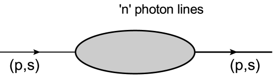
Figure 1: Basic diagram representing the sum of all diagrams of $O(e^{2n})$ in Fock state and CSB

The graphical representation of the blob is shown in Fig. 1. $T^{(n)}$ will be assumed to be IR divergence free.

IV An Example: Cancellation of Infrared divergences up to fourth order

Before presenting the all order proof, we will first revisit the proof of cancellation of IR divergences in $\delta m^{2}$ up to $O(e^{4})$ to illustrate our strategy. In Ref. JAI12 , JAI13 we showed that the true infrared divergences in $\delta m^{2}$ get cancelled up to $O(e^{4})$ if one uses CSB instead of Fock basis to calculate the transition matrix elements JAI12 . Now we sketch the proof for the same based on graphical method which will be generalized to all orders in the next section. For the sake of simplicity, we will consider the contribution due to the 3$-$point interaction terms only.

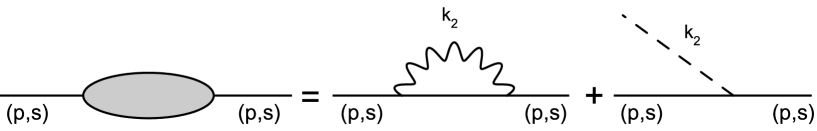
Figure 2: IR finite $O(e^{2})$ blob which represents the sum of Fock state and coherent state contributions

To begin with, consider the $O(e^{2})$ corrections which are represented by the two diagrams on the r.h.s. of Fig. 2. It has been shown in Ref. JAI12 , JAI13 that the sum of these two is IR finite. In our notation, it is equal to

$$T^{(2)}=\sum_{j}\frac{\overline{u}(p,s)\mathcal{M}_{2}^{(j)}u(p,s)}{\mathcal{D}^{(j)}}$$ (18)

where the sum runs over 1 and 2 corresponding to the two diagrams. The sum is represented by the IR finite blob on the l.h.s. in Fig. 2.

Now consider the two diagrams on the r.h.s. of Fig. 3, which are actually Fig. 3(a) and 8(b) in Ref. JAI12 and have been shown to be equal to

Figure 3: IR finite $O(e^{2})$ blob with an external photon line results into $O(e^{4})$ diagram in Fock basis

$$T_{3b}^{(2)} ={e^{4}\over{(2\pi)^{6}}}\int{{d^{2}{\bf k}_{1\perp}}{d^{2}{\bf k}_{2\perp}}\over 2p^{+}}\int{{dk_{1}^{+}}{dk_{2}^{+}}\over{32k_{1}^{+}k_{2}^{+}p_{1}^{+}p_{2}^{+}p_{3}^{+}}}$$

$$\times\frac{\overline{u}(p,s)[\not{\epsilon}^{\lambda_{1}}(k_{1})(\not{p}_{1}+m)\not{\epsilon}^{\lambda_{2}}(k_{2})(\not{p}_{2}+m)\not{\epsilon}^{\lambda_{2}}(k_{2})(\not{p}_{1}+m)\not{\epsilon}^{\lambda_{1}}(k_{1})]u(p,s)}{(p^{-}-p_{1}^{-}-k_{1}^{-})(p^{-}-p_{2}^{-}-k_{1}^{-}-k_{2}^{-})(p^{-}-p_{1}^{-}-k_{1}^{-})}$$ (19)

and

$$T_{3c}^{(2)} =\frac{e^{4}}{(2\pi)^{6}}\int\frac{d^{2}{\bf k}_{1\perp}d^{2}{\bf k}_{2\perp}}{2p^{+}}\int\frac{dk_{1}^{+}dk_{2}^{+}}{16k_{1}^{+}k_{2}^{+}p_{1}^{+}p_{2}^{+}}$$

$$\times\frac{\overline{u}(p,s)[\not{\epsilon}^{\lambda_{1}}(k_{1})(\not{p}_{1}+m)\not{\epsilon}^{\lambda_{2}}(k_{2})(\not{p}_{1}+m)\not{\epsilon}^{\lambda_{1}}(k_{1})]u(p,s)(p\cdot\epsilon^{\lambda_{2}}(k_{2}))\Theta_{\Delta}(k_{2})}{(p\cdot k_{2})(p^{-}-p_{1}^{-}-k_{1}^{-})(p^{-}-p_{2}^{-}-k_{1}^{-}-k_{2}^{-})}$$ (20)

respectively. Here, $p_{1}=p-k_{1}$ and $p_{2}=p-k_{1}-k_{2}$. The sum of Eqs. (IV) and (IV) in our new notation is,

$$T_{3a}^{(2)} =T_{3b}^{(2)}+T_{3c}^{(2)}$$

$$=\frac{e^{2}}{(2\pi)^{3}}\int\frac{d^{3}k_{1}}{2k_{1}^{+}}\frac{\overline{u}(p,s)\epsilon\hbox to0.0pt{\hss/}(k_{1})(\not{p}_{1}+m)\mathcal{M}_{2}^{(j)}(\not{p}_{1}+m)\epsilon\hbox to0.0pt{\hss/}(k_{1})u(p,s)}{(p\cdot k_{1})^{2}\mathcal{D}^{(j)}}$$ (21)

Note that the l.h.s. of Fig. 2 minus the external lines is $\mathcal{M}_{2}^{(j)}$ for the jth diagram and hence the sum of the two $O(e^{4})$ diagrams on the r.h.s. of Fig. 3 is represented by Eq. (IV).

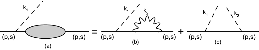
Figure 4: IR finite $O(e^{2})$ blob with an external photon line results into $O(e^{4})$ diagram in coherent basis

Since the blob is IR finite, the IR divergences can appear “only” from the vanishing energy denominators of the kind $(p^{-}-k_{1}^{-}-(p-k_{1})^{-})$. All the other energy denominators inside the blob, which depend on $k_{1}$ and $k_{2}$ need not be taken into account.

Similarly, in CSB, the r.h.s of Fig. 4 is Fig. 8(a) and 9(d) of Ref. JAI12 and which were shown to be equal to

$$T_{4b}^{(2)} ={e^{4}\over{(2\pi)^{6}}}\int{{d^{2}{\bf k}_{1\perp}}{d^{2}{\bf k}_{2\perp}}\over 2p^{+}}\int{{dk_{1}^{+}}{dk_{2}^{+}}\over{32k_{1}^{+}k_{2}^{+}p_{1}^{+}p_{2}^{+}p_{1}^{+}}}$$

$$\times\frac{\overline{u}(p,s)[\not{\epsilon}^{\lambda_{2}}(k_{2})(\not{p}_{2}+m)\not{\epsilon}^{\lambda_{2}}(k_{2})(\not{p}_{1}+m)\not{\epsilon}^{\lambda_{1}}(k_{1})]u(p,s)(p\cdot\epsilon(k_{1}))\Theta_{\Delta}(k_{1})}{(p^{-}-p_{1}^{-}-k_{1}^{-})(p^{-}-p_{3}^{-}-k_{2}^{-})(p^{-}-p_{1}^{-}-k_{1}^{-})}$$ (22)

and

$$T_{4c}^{(2)} =-{e^{4}\over{(2\pi)^{6}}}\int{{d^{2}{\bf k}_{1\perp}}{d^{2}{\bf k}_{2\perp}}\over 2p^{+}}\int{{dk_{1}^{+}}{dk_{2}^{+}}\over{32k_{1}^{+}k_{2}^{+}p_{1}^{+}p_{2}^{+}p_{1}^{+}}}$$

$$\times\frac{\overline{u}(p,s)[\not{\epsilon}^{\lambda_{2}}(k_{2})(\not{p}_{1}+m)\not{\epsilon}^{\lambda_{1}}(k_{1})]u(p,s)(p\cdot\epsilon(k_{1}))(p\cdot\epsilon(k_{2}))\Theta_{\Delta}(k_{1})\Theta_{\Delta}(k_{2})}{(p^{-}-p_{1}^{-}-k_{1}^{-})(p^{-}-p_{3}^{-}-k_{1}^{-})(p^{-}-p_{3}^{-}-k_{2}^{-})}$$ (23)

respectively. Here, $p_{3}=p-k_{2}$. An additional contribution in CSB is obtained by adding Eqs. (IV) and (IV) and will be represented in our new notation as

$$T_{4a}^{(2)}=-\frac{e^{2}}{(2\pi)^{3}}\int\frac{d^{3}k_{1}}{2k_{1}^{+}}\frac{\overline{u}(p,s)\mathcal{M}_{2}^{(j)}(\not{p}_{1}+m)\epsilon\hbox to0.0pt{\hss/}(k_{1})u(p,s)(p\cdot k_{1})}{(p\cdot k_{1})^{2}\mathcal{D}^{(j)}}$$ (24)

and is represented graphically by the l.h.s. of Fig. 4, while the r.h.s. is the sum of Eqs. (IV) and (IV). In the limit, $k_{1}^{+}\rightarrow 0,{\bf k}_{1\perp}\rightarrow 0$, the numerator of Eqs. (IV) and (24) become equal and the sum of their contributions is IR finite. At $O(e^{4})$, there are two other diagrams involving only the three point vertices which contribute to self energy correction. A similar argument can be constructed for the remaining two diagrams as well. The cancellation of IR divergences of these remaining diagrams is illustrated graphically in Fig. 5.

Figure 5: Additional diagrams corresponding to $O(e^{4})$ contributions in Fock basis and CSB.

V Cancellation of Infrared divergences to all orders

Now, we consider an $O(e^{2n})$ blob which we will assume to be free of IR divergences.

Figure 6: Addition of a photon line to $O(e^{2n})$ blob in Fock basis

We shall show that the cancellation of IR divergences in $O(e^{2(n+1)})$ contribution to fermion mass renormalization in LFQED follows from this assumption. To construct an $O(e^{2(n+1)})$ diagram in Fock basis, we can add a photon to $n^{th}$ order blob in three different ways as shown in Fig. 6. The contributions coming from the diagram in Figs. 6(a) and (b), in the limit $q^{+}\rightarrow 0,{\bf q_{\perp}}\rightarrow 0$ are given by

$$T^{(n+1)}_{6a}= \frac{e^{2}}{(2\pi)^{3}}\int\frac{d^{3}q}{2q^{+}}\frac{\overline{u}(p,s)\epsilon\hbox to0.0pt{\hss/}(q)(\not{P}+m)\mathcal{M}_{n}^{(j)}(\not{P}+m)\epsilon\hbox to0.0pt{\hss/}(q)u(p,s)}{(p\cdot q)^{2}\mathcal{D}^{(j)}}$$ (25)

$$T^{(n+1)}_{6b}= -\frac{e^{2}}{(2\pi)^{3}}\int\frac{d^{3}q}{2q^{+}}\frac{\overline{u}(p,s)\epsilon\hbox to0.0pt{\hss/}(q)(\not{P}+m)\epsilon\hbox to0.0pt{\hss/}(q)(\not{p}^{\prime}+m)\mathcal{M}_{n}^{(j)}u(p,s)}{(p\cdot q)(p^{-}-p^{\prime-})\mathcal{D}^{(j)}}$$ (26)

where $P=p-q$ and $p^{\prime}=p$.

Figure 7: Addition of a photon line to $O(e^{2n})$ blob in CSB

The additional contributions in $(n+1)^{th}$ order, when we use the CSB, are shown in Fig. 7 and are given by

$$T^{\prime(n+1)}_{7a}= -\frac{e^{2}}{(2\pi)^{3}}\int\frac{d^{3}q}{2q^{+}}\frac{\overline{u}(p,s)\mathcal{M}_{n}^{(j)}(\not{P}+m)\epsilon\hbox to0.0pt{\hss/}(q)u(p,s)(p\cdot\epsilon(q))\,\Theta_{\Delta}(q)}{(p\cdot q)^{2}\mathcal{D}^{(j)}}$$ (27)

$$T^{\prime(n+1)}_{7b}= \frac{e^{2}}{(2\pi)^{3}}\int\frac{d^{3}q}{2q^{+}}\frac{\overline{u}(p,s)\epsilon\hbox to0.0pt{\hss/}(q)(\not{p}^{\prime}+m)\mathcal{M}_{n}^{(j)}u(p,s)(p\cdot\epsilon(q))\,\Theta_{\Delta}(q)}{(p\cdot q)(p^{-}-p^{\prime-})\mathcal{D}^{(j)}}$$ (28)

In the limit, $q^{+}\rightarrow 0$, ${\bf q}_{\perp}\rightarrow 0$, $(\not{P}+m)\epsilon\hbox to0.0pt{\hss/}(q)u(p,s)\rightarrow(p\cdot\epsilon(q))u(p,s)$. As a result, the sum of Eqs. (25) and (26) exactly cancels the sum of Eqs. (27) and (28). i.e. the IR divergences in Figs. 6(a) and 6(b) are exactly cancelled by those in Figs. 7(a) and 7(b).

VI Overlapping diagrams

The overlapping diagrams as in Figs. 6(c) and 7(c) need a special treatment as in this case attaching a photon line inside the blob changes the structure of the numerator and denominators and thus the blob presented for calculating Figs. 6(a), 6(b), 7(a) and 7(b) in the previous section is different from the one shown in Figs. 6(c) and 7(c). It can be shown that when a photon is absorbed by an IR finite blob, we need to consider only the IR divergences in the limit $q^{+}\rightarrow 0$, ${\bf q}_{\perp}\rightarrow 0$. The general structure of an overlapping diagram is of the form

$$T^{(n+1)}_{6c}= \frac{e^{2}}{(2\pi)^{3}}\int\frac{d^{3}q}{2q^{+}}\frac{\overline{u}(p,s)\mathcal{M}_{n}^{\ell(j)}(\not{P}+m)\epsilon\hbox to0.0pt{\hss/}(q)u(p,s)}{(p\cdot q)\mathcal{D}^{(j)}}$$ (29)

where $\mathcal{M}_{n}^{\ell(j)}$ is $\mathcal{M}_{n}^{(j)}$ with an extra $q$ attached at the $\ell^{th}$ vertex inside the blob as shown in Fig. 6(c). $\mathcal{M}_{n}^{\ell(j)}$ can be written explicitly as;

$$\mathcal{M}_{n}^{\ell(j)}=\epsilon\hbox to0.0pt{\hss/}(k_{1})(\not{P}_{1}+m)\epsilon\hbox to0.0pt{\hss/}(k_{2})(\not{P}_{2}+m)\cdots\cdots\epsilon\hbox to0.0pt{\hss/}(k_{\ell})(P_{\ell}+m)\epsilon\hbox to0.0pt{\hss/}(q)\epsilon\hbox to0.0pt{\hss/}(p_{\ell+1}+m)\cdots\cdots\cdots$$ (30)

The energy denominators corresponding to the intermediate states will be

$$\mathcal{D}^{(j)}=(p^{-}-p_{1}^{-}-k_{1}^{-}-q^{-})(p^{-}-p_{2}^{-}-k_{1}^{-}-k_{2}^{-}-q^{-})\cdots\cdots(p^{-}-p_{\ell}^{-}-\sum_{i}k_{i}^{-}-q^{-})\cdots\cdots\cdots$$ (31)

The coherent state diagram corresponding to the case in which $q$ is emitted at $\ell^{th}$ vertex in the blob is given by

$$T^{\prime(n+1)}_{7c}= -\frac{e^{2}}{(2\pi)^{3}}\int\frac{d^{3}q}{2q^{+}}\frac{\overline{u}(p,s)\mathcal{M}_{n}^{(j)}u(p,s)(p\cdot\epsilon(q))\,\Theta_{\Delta}(q)}{(p\cdot q)\mathcal{D}^{(j)}}$$ (32)

$T^{\prime(n+1)}_{7c}$ gives equal and opposite contribution to Eq. (29). There can be additional $(n-1)$ such overlapping diagrams both in fock and corresponding coherent state bases. Each of the fock state contribution cancels the corresponding coherent state basis contribution at $O(e^{2(n+1)})$ i.e. the sum of Eq. (29) and (32) is infrared finite.

It is to be noted that even if the blob contains 4–point instantaneous vertices, Figs. 6 and 7 are the only diagrams in next order in graphical notation and therefore, the argument presented in this section still holds.

VII Conclusion

We have demonstrated, using the coherent state formalism, that the true IR divergences in self energy correction cancel to all order in LFQED. The proof presented here can be extended to a general n-point amplitude. We plan to address this problem in future.

It is well known that in QCD the IR divergences are not cancelled. One can apply the same procedure as in QED to QCD as shown in ANU00 , BUT78 but then one must obtain the coherent states which incorporate large distance limit of QCD potential. As we know that, in QCD, the in and out states are nothing but the bound states of quarks and gluons, hence one needs to use the method of asymptotic dynamics carefully. One must add to the free Hamiltonian not just the large distance limit of QCD potential but also the confining potential which arises due to the bound state of quarks and gluons in the hadrons. This is the reason why the coherent state formalism was found to be insufficient for the cancellation of IR divergences in higher orders in equal time QCD. The non-cancellation of IR divergences in QCD turns out to be an interesting puzzle, which if solved will help to understand the color confinement properties in QCD. We hope that form of artificial confining potential is the key to the puzzle and will also help us to device an all order proof in QCD. We hope that the coherent state formalism may provide a hint towards constructing an artificial potential for QCD which can be used to perform bound state calculationsWILSON94 .

This is due to the fact that the asymptotic states in strong interactions are bound states and not just the coherent states as in QED. One way to obtain the ”artificial” confining potential required for light front bound state calculations WILSON94 would be to impose the criteria of IR cancellation to find an appropriate potential ANU05 . The techniques developed in present work are expected to play an important role in this.

VIII Acknowledgement

AM would like to thank BRNS for financial support under the Grant No. 2010/37P/47/BRNS and JM would like to thank Department of Physics, Mumbai University.

References

- [1] K. G. Wilson, T. S. Walhout, A. Harindranath, W. -M. Zhang, R. J. Perry and S. D. Glazek, Phys. Rev. D 49, 6720 (1994) [hep-th/9401153].
- [2] S. J. Brodsky, H. -C. Pauli and S. S. Pinsky, Phys. Rept. 301, 299 (1998) [hep-ph/9705477].
- [3] F. Bloch and A. Nordsieck, Phys. Rev. 52, 54 (1937).
- [4] D. R. Yennie, S. C. Frautschi and H. Suura, Annals Phys. 13, 379 (1961).
- [5] V. Chung, Phys. Rev. 140, B1110 (1965).
- [6] P. P. Kulish and L. D. Faddeev, Theor. Math. Phys. 4, 745 (1970).
- [7] M. Greco, F. Palumbo, G. Pancheri-Srivastava and Y. Srivastava, Phys. Lett. B 77, 282 (1978).
- [8] A. Harindranath and J.P. Vary, Phys. Rev. D 37, 3010 (1988).
- [9] L. Martinovic and J.P. Vary, Phys. Lett. B 459, 186 (1999).
- [10] A. Misra, Phys. Rev. D 50, 4088 (1994) [hep-th/9311101].
- [11] A. Misra, Phys. Rev. D 62, 125017 (2000).
- [12] J. D. More and A. Misra, Phys. Rev. D 86, 065037 (2012) [arXiv:1206.3097 [hep-th]]
- [13] J. D. More and A. Misra, Phys. Rev. D 87, 085035 (2013) [arXiv:1302.3522 [hep-th]].
- [14] A. Misra, Phys. Rev. D 53, 5874 (1996).
- [15] D. R. Butler and C. A. Nelson, Phys. Rev. D 18, 1196 (1978); C. A. Nelson, Nucl. Phys. B 181, 141 (1981); C. A. Nelson, Nucl. Phys. B 186, 187 (1981).
- [16] D. Mustaki, S. Pinsky, J. Shigemitsu and K. Wilson, Phys. Rev. D 43, 3411 (1991).
- [17] A. Misra, Few Body Syst. 36, 201 (2005).