Diagnosis of Magnetic and Electric Fields
of Chromospheric Jets through Spectropolarimetric
Observations of H I Paschen Lines

Abstract

Magnetic fields govern the plasma dynamics in the outer layers of the solar atmosphere, and electric fields acting on neutral atoms that move across the magnetic field enable us to study the dynamical coupling between neutrals and ions in the plasma. In order to measure the magnetic and electric fields of chromospheric jets, the full Stokes spectra of the Paschen series of neutral hydrogen in a surge and in some active region jets that took place at the solar limb were observed on May 5, 2012, using the spectropolarimeter of the Domeless Solar Telescope at Hida observatory, Japan. First, we inverted the Stokes spectra taking into account only the effect of magnetic fields on the energy structure and polarization of the hydrogen levels. Having found no definitive evidence of the effects of electric fields in the observed Stokes profiles, we then estimated an upper bound for these fields by calculating the polarization degree under the magnetic field configuration derived in the first step, with the additional presence of a perpendicular (Lorentz type) electric field of varying strength. The inferred direction of the magnetic field on the plane of the sky (POS) approximately aligns to the active region jets and the surge, with magnetic field strengths in the range $10\,\mathrm{G}<B<640\,\mathrm{G}$ for the surge. Using magnetic field strengths of $70$, $200$, and $600\,\mathrm{G}$, we obtained upper limits for possible electric fields of $0.04$, $0.3$, and $0.8\,\mathrm{V\,cm^{-1}}$, respectively. This upper bound is conservative, since in our modeling we neglected the possible contribution of collisional depolarization. Because the velocity of neutral atoms of hydrogen moving across the magnetic field derived from these upper limits of the Lorentz electric field is far below the bulk velocity of the plasma perpendicular to the magnetic field as measured by the Doppler shift, we conclude that the neutral atoms must be highly frozen to the magnetic field in the surge.

1 Introduction

Magnetic fields govern the plasma dynamics in the outer layers of the solar atmosphere. The magnetic energy built up by convection in and below the photosphere is transferred from the photosphere into the heliosphere. During the transfer of energy into the outer layers of the solar atmosphere, i.e., chromosphere and corona, the magnetic energy is partially converted into plasma kinetic energy, causing various active phenomena in the solar atmosphere. Thus the measurement of the magnetic field is of crucial importance to identify the mechanisms responsible for the dynamical phenomena in the solar atmosphere.

Several processes can generate polarization in spectral lines in response to the presence of magnetic and electric fields in the radiation emitting plasma. The Zeeman and Stark effects are produced by the energy separation of the atomic levels into multiple sublevels due to the potential energy of the radiating atom in the external fields. As the splitted components have different polarization properties, this results in a wavelength dependent polarization across the spectral line. In the absence of velocity or field gradients in the emitting plasma, the broadband (i.e., wavelength integrated) polarization from the Zeeman and Stark effect vanishes. In contrast, in the presence of atomic polarization (i.e., population imbalances and quantum interference among the magnetic sublevels; e.g., Landi Degl’Innocenti & Landolfi 2004), the emitted (scattered) radiation is typically characterized by a non-vanishing broadband polarization. The two dominant characteristics of atomic polarization are atomic alignment and orientation. Atomic alignment is a state of population imbalances between magnetic sublevels with different absolute values of their magnetic quantum numbers. Atomic orientation is characterized by population imbalances between sublevels with positive and negative magnetic quantum numbers. The effects of atomic alignment and orientation in the scattered radiation are observed in the form of broadband linear and circular polarization, respectively. In the process of radiation scattering, the anisotropy of the incident radiation field produces atomic alignment, and the scattered light is therefore linearly polarized, with a magnitude depending on the scattering geometry. The presence of a magnetic or electric field produces a relaxation of the atomic coherence among the magnetic sublevels resulting in a modification of the polarization (typically, depolarization and rotation) of the scattered radiation, known as the Hanle effect. Strong magnetic or electric fields also cause a conversion of atomic alignment into atomic orientation when the energy splitting of the sublevels induced atomic level crossings (A-O mechanism, Lehmann, 1964; Landi Degl’Innocenti, 1982; Kemp et al., 1984; Favati et al., 1987; Casini, 2005). Collisions of the scattering atoms with free electrons and protons tend to reduce the atomic level polarization. For the typical density of the upper solar chromosphere, collisional transitions between the fine-structure levels pertaining to the same Bohr level of the neutral hydrogen may play a significant role in the depolarization process (Bommier et al., 1986; Sahal-Br${\rm\acute{e}}$chot et al., 1996; ${\rm\check{S}t\check{e}p\acute{a}n}$ & Trujillo Bueno, 2011).

Recent progress in the modeling of scattering polarization (Trujillo Bueno et al., 2002; L$\acute{{\rm o}}$pez Ariste & Casini, 2002; Trujillo Bueno & Asensio Ramos, 2007) and in the development of increasingly sensitive spectropolarimetric instrumentation (e.g. Collados et al., 2007; Jaeggli et al., 2010; Anan et al., 2012) enables us to measure the chromospheric magnetic field by interpreting the observed polarization in terms of the Zeeman and Hanle effects. Recently, the magnetic field of some types of chromospheric phenomena have been measured, for instance, in filaments (Trujillo Bueno et al., 2002), prominences (Casini et al., 2003; Merenda et al., 2006; Sasso et al., 2011), spicules (L$\acute{{\rm o}}$pez Ariste & Casini, 2005; Trujillo Bueno et al., 2005), and in regions of emerging magnetic flux (Lagg et al., 2004).

Chromospheric jets called “surges” often occur near sunspots, in the proximity of neutral points of the magnetic fields (Rust, 1968), in flux emergence regions (Kurokawa, 1988), or in association with magnetic flux cancellation (Gaizauskas, 1996). They reach heights up to 200 Mm and velocities of 50 to 200 km s^-1 (Roy, 1973). Recent observations have found tiny chromospheric jets outside sunspots in active regions (Shibata et al., 2007; Morita et al., 2010); their typical length and velocity are 1 to 4 Mm and 5 to 20 km s^-1, respectively (Nishizuka et al., 2011). In addition, jet-like features are observed in sunspot penumbrae where stronger, inclined magnetic fields and weaker, nearly horizontal magnetic fields co-exist at small spatial scales (Katsukawa et al., 2007). These jets are interpreted as the result of magnetic energy release caused by a change of magnetic field topology (e.g. Shibata et al., 2007; Ryutova et al., 2008; Nakamura et al., 2012; Takasao et al., 2013). However, there are no studies reporting direct measurements of the magnetic field of jets in the chromospheric lines.

Unlike the measurement of magnetic fields, the study of electric fields in solar plasmas has been given little attention. This is partially due to the fact that appreciable quasi-static electric fields on macroscopic spatial scales are unlikely in the solar atmosphere, since the relaxation time for the electric charge is very short in the highly conductive solar atmosphere. Electric fields generated in magnetic reconnection events occur at spatial scales far smaller than the spatial resolution of current spectropolarimetric instrumentation. On the other hand, the spatial scale of Lorentz electric fields associated with plasma motions across the magnetic field can be large enough to be resolved with existing solar telescopes, and the associated Stark effect can be detected in a weakly ionized plasma that is able to reach sufficient bulk velocities across the magnetic field.

Since detection of the electric field experienced by neutral atoms moving across the magnetic field can tell us about the degree of dynamical coupling between the neutrals and the ionized plasma, the observation and detection of these motional electric fields is of particular interest for understanding the dynamics of partially ionized plasmas in the chromosphere.

In order to possibly detect electric fields, we carried out spectropolarimetric observations of the high Paschen series (i.e., large principal quantum number of the upper level) of neutral hydrogen. The choice of hydrogen was motivated because the linear Stark effect (a first order perturbation of the atomic level energy) only occurs in hydrogen-like ions, whereas multi-electron atoms tend to show only quadratic (and higher order) energy effects in the presence of an external electric field. In the case of the linear Stark effect, the splitting of the energy levels is also roughly proportional to the square of the principal quantum number (e.g. Moran & Foukal, 1991; Foukal & Behr, 1995), so the use of high transitions in a hydrogen line series is desirable in order to increase the magnitude of the polarization signal. Moran & Foukal (1991) and Foukal & Behr (1995) estimated the electric field in post flare loops and prominences by studying the line width variation of the linear polarization profile between two orthogonal states of polarization. The implicit assumption in that study was that atomic polarization of such highly excited initial levels could be neglected since they should mainly be populated by isotropic recombination processes (Casini & Foukal, 1996). Foukal & Behr (1995) measured a surge that occurred in association with a solar flare and obtained a value of the electric field of $\sim 35\,\mathrm{V\,cm^{-1}}$.

Formalisms for the description of hydrogen line polarization in the simultaneous presence of magnetic and electric fields in both local thermodynamic equilibrium (LTE) (Casini & Landi Degl’Innocenti, 1993) and non-LTE including atomic polarization (Casini, 2005) have been developed. In LTE, an electric field of the order of 1 V cm^-1 produces a linear polarization of the order of 0.1% through the linear Stark effect. Casini (2005) pointed out that if an electric field is present in the non-LTE scattering process, magnetic field strengths of order of 10 G can produce a significant level of atomic orientation through the A-O mechanism, comparable to that produced by a magnetic field of the order of 10³ G in the absence of an electric field. This is because, in the presence of an electric field, magnetic-induced level crossing can happen between $\Delta L=1$ levels that are separated in energy by a difference comparable to the Lamb shift, rather than by the much larger L-S coupling fine structure energy separation. In the scattering process with both magnetic and electric fields, an electric field of the order of 0.1 V cm^-1 is sufficient to modify the linear polarization of the observed Paschen lines by about 1%.

Gilbert et al. (2002) evaluated the drain speed of neutral atoms across the magnetic field in a simple prominence model with a partially ionized plasma, in which the solar gravitational force balances with the frictional force proportional to the relative flow of the neutral and ionized components. Their analytical calculations in steady state show the downflow velocity of neutral hydrogen to be $\sim 1.6\,\mathrm{km\,s^{-1}}$ for a density of $10^{10}\,\mathrm{cm^{-3}}$, assuming a ionization fraction of hydrogen of $10^{-3}$ and a ionization fraction of helium of $10^{-2}$. If we assume a magnetic field strength of $100\,\mathrm{G}$, the electric field experienced by neutral atoms moving across the magnetic field is $\sim 0.16\,\mathrm{V\,cm^{-1}}$, and it is possible that the electric field modifies the polarization of the scattered radiation. In dynamic phenomena, electric fields can be stronger than in the steady state case. For instance, the neutral hydrogen in a surge is ejected with a velocity of 50 to 200 km s^-1 with a whiplike motion (Roy, 1973; Nishizuka et al., 2008), while neutral hydrogen in prominences descends and rises along vertical threads with a velocity of 5 to 20 km s^-1 (Zirker et al., 1998; Berger et al., 2008).

In order to study the magnetic and electric fields in chromospheric jets, we observed the full Stokes spectra of the Paschen series of H I in active region jets that took place on the solar limb on May 5, 2012. For convenience, throughout this paper we use the two terms “surge” and “jet” to refer to large and small events, respectively. In the following sections, we describe the details of the observations (Sec. 2), the inference of the magnetic and possible electric fields (Sec. 3), and finally we discuss our measurements and provide our conclusions (Sec. 4).

2 Observations and data reduction

Several jets in the active region NOAA 11476 were observed in several H I Paschen lines using the universal spectropolarimeter (Anan et al., 2012) of the Domeless Solar Telescope (Nakai & Hattori, 1985) at Hida observatory, Japan. The polarimeter uses a continuously rotating achromatic waveplate as polarization modulator and provides the full Stokes vector of any spectral regions between 4000 Å and 11000 Å for all the spatial points along the spectrograph slit, with a spatial sampling of $\sim 0.4$ arcsec/px. The full Stokes spectra so obtained were calibrated for instrumental polarization using a predetermined Mueller matrix of the telescope. The expected error on the determination of a given Stokes polarization parameter $S=Q,U,V$, can be expressed as (Ichimoto et al., 2008; Anan et al., 2012)

$$\delta\Biggl{(}\frac{S}{I}\Biggr{)}=a\,\frac{S}{I}+\sigma$$ (1)

where $a$ is the polarimetric accuracy of the calibration and $\sigma$ is the rms polarimetric sensitivity of the observation, which is measured by the statistical noise with respect to the peak intensity of the spectral line. Our calibration procedure guarantees that $|a|\lesssim 0.05$. Estimates of $\sigma$ for the different Paschen lines in our observations are given in the next paragraph.

The observation ran from 2:32 UT to 3:50 UT on 2012 May 5. Two beams with orthogonal polarizations are taken simultaneously with a CCD camera (Prosilica GE1650) with a spectral sampling of 70 mÅ/pix and an exposure time of 500 msec, and 99 frames are integrated in 49.5 sec, while the spin rate of the rotating waveplate is 0.1 rev./sec. Full Stokes spectra were observed in “sit-and-stare” mode for all P$n$ lines of the Paschen series of H I, for the values $n=7,9,10,11,12,13,15,18,19,20$ of the principal quantum number of the upper level. These lines were observed sequentially by rotating the spectrograph grating. The rms polarization sensitivity for the strongest lines P7, P9, P10, P11, P12, and P13, was estimated to be, respectively, $\sim 2\times 10^{-3}$, $2\times 10^{-3}$, $3\times 10^{-3}$, $3\times 10^{-3}$, $3\times 10^{-3}$, and $4\times 10^{-3}$. We did not analyze the Stokes spectra for the Paschen lines above P15, because the observed signals were lower than 10% of the scattered continuum outside the solar limb, and were thus dominated by flat field errors. The line wavelengths were determined by identifying neighboring absorption lines in the background scattered spectrum in the solar atlas of Kurucz et al. (1984). Because motion of the solar image on the slit caused by the seeing and telescope guiding error was approximately $1$ arcsec in amplitude during the run of the observation, we averaged the Stokes spectra in the spatial direction over 2 arcsec. The properties of the observed data set are summarized in Table 1.

The slit was placed outside the solar limb, approximately parallel to it, above active region NOAA 11476. The slit width and length were 1.28 arcsec and 128 arcsec, respectively. In our analysis, the slit identifies the reference direction of polarization, along which Stokes $Q$ is defined to be positive.

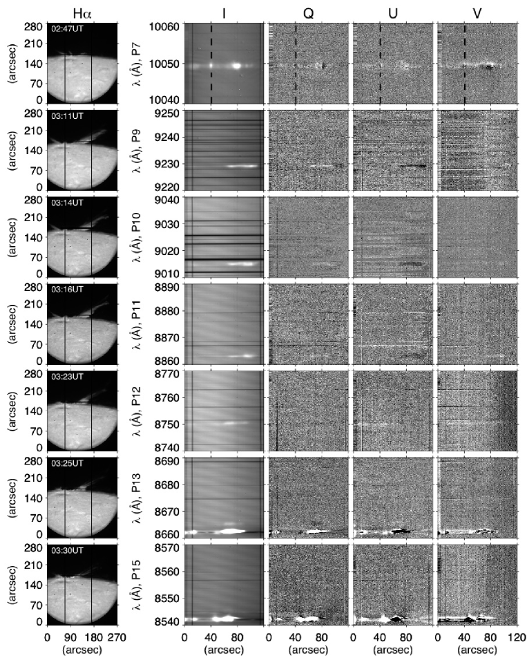
Figure 1: Observed Stokes spectra of the Paschen series of neutral hydrogen (4 right columns) and slit-jaw images in H$\alpha$ (left column). The data set in each row were obtained simultaneously. The horizontal lines in the slit-jaw images show the spectrograph slit. The two vertical lines in the slit-jaw images and the $I$ spectral images show the spectrograph hairlines. The vertical dashed lines in the Stokes spectra of the P7 denote the location of the profiles shown in Figure 2. The strong emissions features in the frames of P13 and P15 are the Ca II 8662Å and Ca II 8542Å lines, respectively.

Figure 1 shows examples of the observed Stokes spectra of the P7, P9, P10, P11, P12, P13, and P15 lines with slit-jaw images taken at the H$\alpha$ line center. In the spectral ranges of P13 (8665 Å) and P15 (8545 Å) there are strong emission lines of Ca II 8662 Å and Ca II 8542 Å, whose peaks are strongly saturated. During the observation, some jets and a surge took place across the slit. The jets were observed in P7 between 2:32 UT and 2:47 UT, while the surge was observed in the P9, P10, P11, P12, P13, P15, P18, P19, and P20 during the second half of the observation period. The distance of the slit to the visible limb for the observation of the jets and the surge was, respectively, $\sim 10$ arcsec and $\sim 15$ arcsec.

After correcting our data for instrumental polarization, the Stokes spectra still show a residual polarization signal in the continuum around the Paschen lines. This is likely caused by stray light in the instrument, and indicates that the line signal in the jets and surge is also affected by this spurious polarization. We simply corrected for it by subtracting the polarization offset that is obtained by averaging the Stokes signal in spatial positions along the slit outside the detectable emissions of Paschen lines. These signals are typically dominated by the scattered photospheric spectrum, showing evidence of absorption features in the spectral region of interest. However, in the stray light spectra observed in our data, the photospheric signal of the Paschen lines is not distinguishable.

We also cannot exclude that part of the spurious polarization offset may be due to residual polarization cross-talk from Stokes $I$ after the polarization calibration. In particular, this could be caused by imperfect spatial coregistration and/or intensity rescaling of the two beams with orthogonal polarizations before subtraction. Some evidence of this can be glimpsed from the Stokes $Q$, $U$, and $V$ spectra of Figure 1, as some of these spectra clearly show a spurious signal in correspondence with the slit-jaw hairlines. We take into account this possibility in Sec. 3.4, when we estimate the effects of possible Lorentz fields on the polarization of the observed lines.

3 Diagnosis of magnetic and electric fields

Figure 1 and 2 show the observed Stokes spectra of the Paschen series of H I and an example of Stokes profiles of P7, respectively. It must be noted that the shape of the linear polarization signals resemble that of the intensity profile. This suggests the presence of atomic polarization in the upper levels of the transitions of neutral hydrogen in the studied jets and surge, and puts into question the assumption that was made in previous studies of electric field measurements by spectro-polarimetric observations, that the atomic polarization of highly excited levels should be negligible (e.g. Foukal & Hinata, 1991; Casini & Foukal, 1996), presuming that these levels are mostly populated by electron recombination. Our observations indicate instead that optically pumped atomic polarization must be significant, at least for the upper levels of the Paschen lines that we considered.

Casini (2005) derived a formalism for modeling the scattering polarization of hydrogen lines in the presence of both magnetic and electric fields. In that work, he predicted that a small electric field of the order of 1 V cm^-1, even if contributing negligible linear polarization via the Stark effect, can still bring important modifications to the atomic polarization of the hydrogen levels when acting in the presence of a magnetic field. In particular, the simultaneous presence of magnetic and electric fields brings an enhancement of the A-O mechanism that is responsible for the appearance of net circular polarization (NCP).

Figure 1 does not show a significant amount of NCP. Since it is not possible to conclude from the data that electric fields may be producing any effect, we carried out the inversion of the Stokes spectra taking into account only the effect of magnetic fields. We then estimated an upper limit for the electric field in the plasma by calculating the polarization degree in the simultaneous presence of magnetic and electric fields, assuming for the magnetic field the configuration derived from the inversion.

3.1 Line formation in the presence of magnetic fields: PCA-based inversion of the observations

The inversion of the full Stokes profiles of the observed Paschen H I lines in the presence of a magnetic field made use of pattern recognition techniques. Such type of inversion involves the search of a precomputed database of Stokes profiles for the best match to the observed profiles. Specifically, we adopted Principal Component Analysis (PCA) for our implementation of pattern recognition inversion (Rees et al., 2000; Socas-Navarro et al., 2001; L$\acute{{\rm o}}$pez Ariste & Casini, 2002).

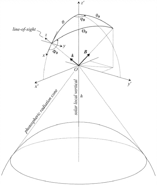
Figure 3: Geometric model for radiation scattering in the presence of a magnetic field. The cone of (photospheric) radiation irradiates the scattering atoms at the point $O$ of height $h$ above the solar surface. The direction of the magnetic field vector, $\mathbf{B}$, is defined by the angles $\vartheta_{B}$ and $\varphi_{B}$ in the reference frame of the local solar vertical through the point $O$, and by $\Theta_{B}$ and $\Phi_{B}$ in the reference frame of the LOS, $\mathbf{k}$. The inclination angle of $\mathbf{k}$ from the local solar vertical is $\vartheta$ and the direction of $y\equiv y^{\prime}$, which corresponds to the reference direction of positive Stokes $Q$, is parallel to the solar limb.

The code computing the inversion database of Stokes profiles solves the statistical equilibrium of a quantum model of the H I atom in the presence of the magnetic field (L$\acute{{\rm o}}$pez Ariste & Casini, 2002; Landi Degl’Innocenti & Landolfi, 2004), and computes from this solution the full Stokes vector of the scattered radiation. Figure 3 shows the geometry of scattering in the presence of the magnetic field, and the parameters used in the line formation code.

For a good inversion, the database must cover the full range of parameters spanning the line formation model. The parameters used to construct the precomputed database are the magnetic field strength, $B$, the inclination of the magnetic field vector with respect to the local solar vertical, $\vartheta_{B}$, the azimuth angle about the local solar vertical with respect to the $x^{\prime}$ axis, $\varphi_{B}$, the inclination of the line-of-sight (LOS) from the local solar vertical, $\vartheta$, the height of the scattering point from the solar surface along the local solar vertical, $h$, the optical thickness of the slab at line center, $\tau$, and the temperature of the plasma in the scattering region, $T$ (Fig. 3). The adopted range of these seven parameters, are $0.01<h<0.08\,R_{\odot}$, $0<B<1000$ G, $0^{\circ}<\vartheta_{B}<180^{\circ}$, $0^{\circ}<\varphi_{B}<360^{\circ}$, $82^{\circ}<\vartheta<98^{\circ}$, $0.01<\tau<1$, and $1000<T<65000$ K.

One of the assumptions of the model is that the incident radiation on the scattering atom is not polarized, and possesses cylindrical symmetry around the local solar vertical through the scatterer. In the approximation of complete redistribution under which the line formation model for this problem is valid, we must also assume that the radiation is spectrally flat over the width of the spectral line. Another assumption is to neglect collisional coupling among the atomic levels. In Sect. 4 we discuss how this approximation affects the inference of the magnetic and electric fields in the plasma.

The emergent Stokes parameters are obtained by solving the radiative transfer equation

$$\frac{d}{ds}\left(\begin{array}[]{c}I\\ Q\\ U\\ V\\ \end{array}\right)=\left(\begin{array}[]{cccc}\eta_{I}&\eta_{Q}&\eta_{U}&\eta_{V}\\ \eta_{Q}&\eta_{I}&\rho_{V}&-\rho_{U}\\ \eta_{U}&-\rho_{V}&\eta_{I}&\rho_{Q}\\ \eta_{V}&\rho_{U}&-\rho_{Q}&\eta_{I}\\ \end{array}\right)\left(\begin{array}[]{c}I\\ Q\\ U\\ V\\ \end{array}\right)+\left(\begin{array}[]{c}\epsilon_{I}\\ \epsilon_{Q}\\ \epsilon_{U}\\ \epsilon_{V}\\ \end{array}\right),$$ (2)

where $s$ is the geometrical distance along the ray passing through a slab and $(\eta_{I},\eta_{Q},\eta_{U},\eta_{V})$, $(\rho_{Q},\rho_{U},\rho_{V})$, and $(\epsilon_{I},\epsilon_{Q},\epsilon_{U},\epsilon_{V})$ represent, respectively, the dichroic absorption, dispersion, and emission coefficients for the Stokes parameters $I$, $Q$, $U$, and $V$. The expression for each of those quantities is given by equations (7.47) of Landi Degl’Innocenti & Landolfi (2004). We assume homogenous physical conditions along the optical depth within the slab. When the anomalous dispersion and dichroism terms are small, $\eta_{I}\gg(\eta_{X},\rho_{X})$ (with $X=Q,U,V$), and the polarized emission is weak, $\epsilon_{I}\gg\epsilon_{X}$, we can formally integrate equation (2), yielding (Trujillo Bueno et al., 2005)

$$I(\tau) = I_{0}e^{-\tau}+\frac{\epsilon_{I}}{\eta_{I}}(1-e^{-\tau})$$

$$X(\tau) = \frac{\epsilon_{X}}{\eta_{I}}(1-e^{-\tau})-I_{0}\frac{\eta_{X}}{\eta_{I}}\tau e^{-\tau}-\frac{\epsilon_{I}\eta_{X}}{\eta_{I}^{2}}[1-e^{-\tau}(1+\tau)],$$

where $\tau$ (with $d{\tau}=-\eta_{I}ds$) is the optical depth along the ray, and $I_{0}$ is the background intensity of the slab (which is zero outside the limb).

The above approximate formulas for the emergent Stokes parameters from a homogeneous and weakly polarizing slab are reasonable for the modeling of solar chromospheric structures (Trujillo Bueno et al., 2005; Trujillo Bueno & Asensio Ramos, 2007).

The adopted atomic model of H I is composed of the terms in L-S coupling of principal quantum numbers $n=1,2,3,4$ plus the value of $n$ pertaining to the upper level of the observed transition. L-S coupling is a reasonably good approximation for light atoms such as H I. The reason for including the $n=4$ level in the atomic model is because of the importance of the H$\alpha$ and H$\beta$ radiation in the solar spectrum in determining the polarization of the $n=2,3,4$ levels. The omission of the intermediate terms between $n=4$ and the upper level of the observed transition is justified because the statistical equilibrium of the upper level must be dominated by the optical pumping through the resonant radiation at the frequency of the observed line from the $n=3$ level, as indicated by the predominance of the atomic polarization signature in the emitted radiation.

Figure 4 shows the estimated polarization degree for Stokes $Q$, $U$, and $V$, of the lines P7, P9, P10, and P11, for the case of $90^{\circ}$-scattering of the solar radiation at the limb. The polarization degree is calculated through $Q/I_{\mathrm{max}}$ and $U/I_{\mathrm{max}}$ at line center in the case of linear polarization, and through the NCP in the case of Stokes $V$, as a function of the magnetic field strength, and for two geometric configurations of the magnetic field. In the first configuration (upper panel), the magnetic field is directed along the LOS. For zero magnetic field, the scattered light is linearly polarized with positive $Q$ (i.e., parallel to the limb) as expected. For $10^{-2}\,\mathrm{G}<B<10\,\mathrm{G}$, the direction of the linear polarization is rotated with respect to the zero-field case, and the degree of polarization is also decreased approaching zero around 10 G. These rotation and reduction of the linear polarization of scattered radition are characteristic phenomena of the magnetic Hanle effect. For $B>1\,\mathrm{G}$, the atomic energy levels within a fine structure term in the upper level start crossing each other, creating the conditions for the Paschen-Back effect and the A-O mechanism to generate asymmetric components in the Stokes $V$ profile as a function of wavelength.

In the second magnetic configuration (lower panel), the magnetic field is perpendicular to the LOS and parallel to the limb. For $10^{-2}\,\mathrm{G}<B<10\,\mathrm{G}$, the Hanle effect only depolarizes the scattered radiation, to about 1/2 of the zero-field value. For $B$ larger than a few $10\,\mathrm{G}$, the generation of linear polarization by anisotropic pumping of radiation becomes more efficient due to the change of energy configuration of the atom in the transition to the Paschen-Back regime (Landi Degl’Innocenti & Landolfi, 2004; Casini & Manso Sainz, 2006), when the spin-orbit interaction becomes negligible with respect to the magnetic interaction.

The fundamental concepts of PCA inversion of Stokes profiles were described by Rees et al. (2000). Applications of this technique to scattering polarization on the Sun were considered by L$\acute{{\rm o}}$pez Ariste & Casini (2002); Casini et al. (2003, 2005, 2009). PCA is mainly a technique for pattern recognition and data compression. It allows an efficient decomposition of the Stokes profiles using only a very small number of “universal” principal components (eigenprofiles) out of the full basis that would be needed for a lossless reconstruction of the profiles. The dimension of the PCA basis equals the number of wavelength points in the profiles. Since the number of principal components needed to reconstruct the Stokes profile to within the polarization sensitivity of the observations is much smaller (typically by at least one order of magnitude) than the number of wavelength points, PCA allows a much faster comparison of the observed data with the model than iterative fitting. Additionally, the use of a precomputed database of profiles for data inversion is free from the risk of converging to local minima typical of iterative fitting.

3.2 Test of the inversion code

We examined the reliability of our inversion scheme by performing test runs for 10,000 synthetic Stokes profiles calculated with randomly distributed parameters in the 7D parameter space within the ranges specified earlier, after adding to the profiles a random noise of $3\times 10^{-3}$ with respect to the peak intensity. The inversion tests were run for P7, P9, P10, and P11, using a database of 100,000 models. Figure 5 shows the inversion results against the actual values of the synthetic model for each parameter, for the case of the P7 line. The results for the inversion of the other lines are similar to the case of P7, and therefore we do not shown them here.

Figure 5b shows the scatter plot of the longitudinal magnetic field strength ($B\,\cos{\Theta_{B}}$). This quantity is determined rather well from the inversion of Stokes $V$, which is mostly affected by the longitudinal Zeeman effect. In contrast, the error in the inversion of the magnetic field strength and the inclination angle of the magnetic field vector is rather large (Figs. 5a and 5c). This can be understood when we consider that, for these Paschen lines, the Hanle effect is completely saturated already for $B>10\,\mathrm{G}$ (Fig. 4), whereas the Zeeman effect does not produce a significant linear polarization until the field reaches strengths of the order of a few kG. Therefore, for $10\lesssim B\lesssim 1000$ G the inferred magnetic field strength is derived mainly from the circular polarization signal.

Since there can be different values of the magnetic field strength corresponding to a given degree of NCP or to the amplitude of the linear polarization induced by anisotropic excitation (Fig. 4), and considering that the atomic alignment from which both these polarization signals originate depends on the true height (versus the observed projected height) of the scatterer over the solar surface, as well as on the inclination of the magnetic field from the local solar vertical $\vartheta_{B}$ (see eqs. [3] below), we can understand why the inference of the magnetic field strength and inclination can be affected by larger errors.

The scatter plot of the inverted azimuth angle of the magnetic field in the reference frame of the observer, $\Phi_{B}$, exhibits multiple streaks, which are caused by intrinsic ambiguities of scattering line polarization with the geometry of the field (Fig. 5d). Typical examples are the well-known $180^{\circ}$-ambiguity of the Zeeman effect, and the $90^{\circ}$-ambiguity of the saturated regime of the Hanle effect (e.g. House, 1977; Casini & Judge, 1999; Casini, 2002; Casini et al., 2005). In order to see this, we consider the emissivity for Stokes $Q$ and $U$ in the saturated regime of the Hanle effect for a two-level atom with unpolarized lower level, and neglecting stimulated emission. This is simply expressed by

$$\left.\begin{array}[]{c}\epsilon_{Q}\sim w(3\cos^{2}{\vartheta_{B}}-1)\sin^{2}{\Theta_{B}}\cos{2\Phi_{B}}\\ \epsilon_{U}\sim w(3\cos^{2}{\vartheta_{B}}-1)\sin^{2}{\Theta_{B}}\sin{2\Phi_{B}}\end{array}\right.,$$ (3)

where $w$ is the anisotropy factor of the radiation field (Casini, 2002). A sign change of Stokes ${\it Q}$ and ${\it U}$ due to a $90^{\circ}$ change of $\Phi_{B}$ can thus be compensated by a sign change of the factor $(3\cos^{2}{\vartheta_{B}}-1)\sin^{2}{\Theta_{B}}$. Therefore the condition for the presence of the $90^{\circ}$ ambiguity (in the optically thin case) is the existence of $\vartheta_{B}^{\prime}$ and $\Theta_{B}^{\prime}$ such that

$$(3\cos^{2}{\vartheta_{B}}-1)\sin^{2}{\Theta_{B}}=-(3\cos^{2}{\vartheta_{B}^{\prime}}-1)\sin^{2}{\Theta_{B}^{\prime}}.$$ (4)

Since the dependence of the Stokes $Q$ and $U$ polarization on the geometry of the field and the observer, as given by eqs. (3), is modified in the optically thick case, or for the case of a multi-level atom, we have checked this dependence numerically in the optically thick case relying on our line formation model. As a result, we verified that the expected variations of the polarization degree of the Paschen series with optical thickness remain below the noise level of the observations, and thus we can still rely on eqs. (3) to provide an approximate description of the azimuthal ambiguities even for our more general atomic and radiative transfer models. In the inversion results (see Sect. 3.3), we determine whether the inferred configuration is subject to ambiguities, by checking whether the condition (4) can be realized for that configuration.

If we ignore the ambiguities shown in Fig. 5d, the 90% confidence interval for the inversion of $\Phi_{B}$ is $\pm 13^{\circ}$ for P7, P9, P10, and P11.

The temperature is inferred from the line width under the assumption that this is determined by thermal broadening. The error on $T$ is estimated to be $0.2\,T$, based on the scatter plot of Fig. 5e.

The determination of the remaining parameters is not very accurate. The optical depth deforms the line shape and slightly changes the polarization degree of the line. The height of the scatterer determines the dilution and anisotropy factors of the incident radiation field, which in turn determines the state of atomic polarization in the zero-field case. However, a change of the height over the entire parameter range, between $0.01$ and $0.08\,R_{\odot}$ causes only small changes in the polarization degree of the lines. The same is true for the change of $\vartheta$ between $82^{\circ}$ and $98^{\circ}$.

3.3 Inversion results

The observed Stokes spectra of the P7, P9, P10, and P11 lines were inverted using the PCA technique illustrated in Sect. 3.1, in order to derive the magnetic and plasma model of the emitting plasma in the observed active region’s jets and surge. We did not invert the Paschen lines above P11, because the signal-to-noise ratios of the polarization signals were too low.

For the inversion, the possible effects of an electric field (e.g., of the Lorentz type) were neglected. The Doppler velocity was derived from the shift of the center of gravity of the Stokes $I$ profiles, using the wavelengths of the Paschen lines as reported by Kramida (2010).

Figure 2 shows an example of inversion fit of the Stokes vector of P7 for a jet, the location of which is indicated by the dashed lines in the top of Fig. 1. Our spectral synthesis does not reproduce the complex shape of Stokes profiles produced in a spatially unresolved, multi-component atmosphere, because of the assumption of a homogeneous slab. Nonetheless, most of the observed Stokes profiles fit satisfactorily some synthetic profile in our inversion database with only 100,000 models, as shown in Fig. 2.

The distributions of the inverted parameters along the slit are shown in Figure 6. The ranges of the physical parameters estimated from the inversion corresponding to the 90% confidence level (Sec. 3.2) are shown in the four bottom rows, respectively for the longitudinal component of the magnetic field, the magnetic field strength, the plasma temperature, and the plasma velocity along the LOS. In the top row, the direction of the lines indicates the direction of the magnetic field on the POS (related to $\Phi_{B}$). The red (blue) color marks the solutions which admit (do not admit) an alternative $90^{\circ}$-ambiguous configuration of the magnetic field. The magnetic field solutions that do not admit this azimuthal ambiguity indicate that the projected magnetic field on the POS is approximately aligned to the jets and the surge. Accordingly, 60% of the solutions marked with the red lines were rotated by 90^∘ in order to align the projected magnetic field on the POS to the directions of the jets and the surge. After this operation, it is noticeable that the direction of the magnetic field on the POS appears to be systematically tilted away from the surge by about $25^{\circ}$ counterclockwise, which is larger than the estimated inversion error of $13^{\circ}$ of $\Phi_{B}$ corresponding to the 90% confidence level. We do not speculate on the physical origin of this tilt.

The inverted magnetic field component along the LOS ($B_{\parallel}=B\cos{\Theta_{B}}$) is comprised in the following ranges, respectively for the three jets and the surge: $0\,\mathrm{G}<B_{\parallel}<180\,\mathrm{G}$, $80\,\mathrm{G}<B_{\parallel}<250\,\mathrm{G}$, $10\,\mathrm{G}<B_{\parallel}<160\,\mathrm{G}$, and $-70\,\mathrm{G}<B_{\parallel}<100\,\mathrm{G}$.

For the magnetic field strength of the three jets, using the observation at 2:47 UT, we found $60\,\mathrm{G}<B<630\,\mathrm{G}$, $190\,\mathrm{G}<B<960\,\mathrm{G}$, and $40\,\mathrm{G}<B<200\,\mathrm{G}$. In the case of the surge, the circular polarization is practically absent, leading to a larger uncertainty in the determination of the magnetic field strength in that structure. For a 90% confidence level we found $10\,\mathrm{G}<B<640\,\mathrm{G}$.

Figure 6 shows other parameters that are determined by the inversion. The derived temperature must be regarded as an upper limit, because only thermal and natural broadening were considered for the inversion, while other broadening mechanisms such as pressure broadening, plasma turbulence, and collisional damping may also contribute to the effective line width. The maximum Doppler velocity of the surge at 3:11 UT, 3:13 UT, and 3:16 UT was $7\,\mathrm{km\,s^{-1}}$, $4\,\mathrm{km\,s^{-1}}$, and $16\,\mathrm{km\,s^{-1}}$, respectively.

3.4 Upper limit of the electric field

The time evolution of the surge can be seen in Figure 7, which shows a slit-jaw image at the line core of H$\alpha$ (left) and two time-distance diagrams showing the motion along two different sections of the surge, respectively parallel (top right) and perpendicular (bottom right) to it.

The surge first appeared at 2:58 UT, ejected at a speed of $\sim 100\,\mathrm{km\,s^{-1}}$, initially with a whiplike motion, finally reaching a length of $\sim 110,000\,\mathrm{km}$. The observations taken at 3:11 UT, 3:13 UT, and 3:16 UT show the surge near its maximum extension. The observed Doppler shift indicates a significant component of plasma velocity along the LOS, which is also nearly perpendicular to the magnetic field, if we accept the inversion results that the magnetic field vector practically lies in the POS (Fig.6). Therefore, this event provides a good opportunity for testing the coupling between partially ionized plasma and magnetic fields, since neutral atoms that move across the magnetic field must experience a motional electric field.

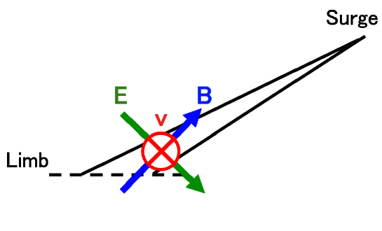
Figure 8: Schematic picture of the magnetic, electric, and velocity vectors in the surge.

We used the inverted magnetic and velocity field configurations of the surge as the basis to calculate the emergent Stokes profiles in the additional presence of an electric field (Fig. 8). The magnetic field, which is roughly aligned to the surge, is inclined about $45^{\circ}$ from the local solar vertical, and on the POS (Fig. 6). The velocity component is assumed to be along the LOS, because no significant apparent lateral motions were observed in the H$\alpha$ slit-jaw images at the times of the observation, 3:11 UT, 3:13 UT, and 3:16 UT (Fig. 7). Since the inferred magnetic field strength in the surge varies approximately between $10\,\mathrm{G}<B<640\,\mathrm{G}$, we calculated the expected line polarizations in the presence of a motional electric field for three magnetic-field strengths of $70$, $200$, and $600\,\mathrm{G}$. Unlike the surge, the magnetic field in the jets has a significant component along the LOS. Since it is difficult to estimate the velocity component across the magnetic field from the time evolution of the plasma in the observations, we omit any discussion about the estimation of electric fields in the jets.

We calculated the theoretical net linear and circular polarizations of the Paschen H I lines as functions of the strength of the motional electric field, assumed to be perpendicular to both the magnetic field and the LOS, using the formalism of Casini (2005). Because of the particular field geometry (both fields lie on the POS), all configurations where the orientation of either of the two fields is inverted give rise to the same polarization.

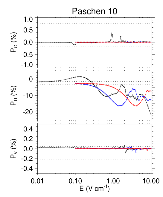
Figure 9: Broadband polarization of P10 in Stokes $Q$ (top), $U$ (center), and $V$ (bottom), as a function of the electric field strength, in a $90^{\circ}$ scattering event. The magnetic field lies on the POS, with azimuth $\Phi_{B}=135^{\circ}$ (see Fig. 3). The electric field also lies on the POS, and is assumed to be perpendicular to the magnetic field. Black, blue, and red lines correspond to magnetic field strengths of $70$, $200$, and $600\,\mathrm{G}$, respectively. The horizontal lines in each plot limit the range of polarization error due to both random and systematic (instrumental stray light and residual polarization cross-talk) sources.

Figure 9 shows the results for P10 for the three selected values of the magnetic field strength. It is notable that the direction of the linear polarization does not change appreciably when the electric field is applied. This is in fact dominated by Stokes $U$ at all times, in agreement with the fact that the atom is in the saturated regime of the (magnetic) Hanle effect, and therefore the direction of linear polarization must be perpendicular to the magnetic field direction ($135^{\circ}$ in this calculation). This fact allows us to determine the azimuth angle of the magnetic field ($\Phi_{B}$) from the inversion independently of the effect of possible electric fields.

The upper limit of the electric field in the P10 at 3:13 UT is estimated by comparing the observed polarization degree with the calculated values. Because of the residual continuum polarization observed in the Stokes spectra after correcting them for instrumental polarization (see end of Sect. 2), the observed polarization degree is affected by both random and systematic errors. In Figure 9, the horizontal dotted lines in each plot limit the range of polarization error due to both systematic (either instrumental stray light or residual polarization cross-talk) and random sources. Additional polarization effects due to an undetected motional electric field must then lie within this range.

We thus find an upper limit of $0.04$, $0.3$, and $0.8\,\mathrm{V\,cm^{-1}}$, respectively for the magnetic field strength of $70$, $200$, and $600\,\mathrm{G}$. This implies that the upper limit of the velocity of neutral hydrogen moving across the magnetic field corresponds respectively to $0.6$, $1.5$, and $1.3\,\mathrm{km\,s^{-1}}$. Since the measured Doppler velocity in the P10 at 3:13 UT is $3.4\pm 1.6\,\mathrm{km\,s^{-1}}$, the velocity of neutral hydrogen moving across the magnetic field appears to be significantly smaller than the plasma’s bulk velocity.

In the same way, we estimated the upper limit of the velocity of neutral hydrogen moving across the magnetic field at 3:11 UT from observations of the P9 line. We found in this case the values $0.8$, $1.5$, and $1.1\,\mathrm{km\,s^{-1}}$ for the same magnetic field strengths, in very good agreement with the results found with P10. Using the P11 data (observed at 3:16 UT) we found instead $1.1$, $1.0$, and $0.8\,\mathrm{km\,s^{-1}}$, which also are in agreement with the results from P9 and P10. Since the measured Doppler velocity in the P9 at 3:11 UT, and in the P11 at 3:16 UT, are $3.3\pm 0.2\,\mathrm{km\,s^{-1}}$ and $12.5\pm 1.4\,\mathrm{km\,s^{-1}}$, respectively, all estimated upper limits of the velocity across the magnetic field are smaller than the measured Doppler velocities.

4 Discussion and summary

We presented magnetic field inferences in a surge and in active region jets, and a first estimation of the upper limit of motional electric fields, and the corresponding limit to plasma velocities across the magnetic field lines.

The direction of the magnetic field on the POS is found to approximately align to the jets and the surge. This confirms the common scenario of the chromospheric jet model, in which plasma is ejected along the magnetic field (e.g. Shibata et al., 2007; Takasao et al., 2013). When we look carefully at the geometric relation between the magnetic field and the jet, we find that the direction of the magnetic field is slightly tilted counterclockwise from the direction of the surge. Further study with high-accuracy spectro-polarimetric data for a number of similar events is needed in order to clarify the details of the geometric relation between the magnetic field and jets.

The strength of the magnetic field in the three jets is found to be in the ranges $60\,\mathrm{G}<B<630\,\mathrm{G}$, $190\,\mathrm{G}<B<960\,\mathrm{G}$, and $40\,\mathrm{G}<B<200\,\mathrm{G}$. This determination is driven mainly by the observed circular polarization signal and its symmetry characteristics. Because NCP can also be generated by the coupling of velocity and magnetic field gradients along the LOS (Illing, 1974), and since our model does not contemplate the possibility of a multi-component atmosphere, we cannot exclude the possibility that the inferred magnetic field strengths may be affected by the possible presence of velocity and magnetic field inhomogeneities along the LOS.

The upper limit of the motional electric field is estimated to be $0.04\,\mathrm{V\,cm^{-1}}$ for a magnetic field strength of $70\,\mathrm{G}$, based on the observed polarization degree in the P10 line. If we neglect the magnetic field and the atomic level polarization, as assumed in previous estimates of solar electric fields, the limit to the electric field that is derived from the observed polarization degree (using, e.g., the formalism of Goto 2008) is $\sim 30\,\mathrm{V\,cm^{-1}}$, which is significantly larger than our estimates.

In our inversion model, we neglected collisional coupling among the atomic levels, which tends to reduce the amount of linear polarization and NCP in the scattered radiation. In the case of the surge, the observed linear polarization may be explained through a combination of collisional depolarization with the polarizing effects of the magnetic field and the possible motional electric fields in the plasma (Fig. 9). In particular this implies that our inferred upper bounds for the motional electric field present in the surge could be underestimated. Similarly, our model might underestimate the LOS component of the magnetic field, if the observed low values of NCP were caused by the destruction of atomic orientation by collisions. Finally, we note that the presence of isotropic collisions does not cause a significant change of the direction of the emergent linear polarization, hence we can still reliably determine the azimuth angle of the magnetic field on the POS ($\Phi_{B}$) from the inversion, independently of the effects of collisions.

From the upper limit of the motional electric field, we can estimate the maximum velocity of neutral hydrogen moving across the ambient magnetic field. At 3:16 UT, the surge reaches its maximum height (Fig. 7) and a large bulk velocity (i.e., Doppler shift) is observed (Fig. 6). Therefore the velocity vector can be assumed to be along the LOS and perpendicular to the magnetic field (Fig. 6). On the other hand, from our analysis of the polarization effects of motional electric fields, the upper limit of the velocity of neutral hydrogen moving across the magnetic field is found to be $1.1\,\mathrm{km\,s^{-1}}$ in this geometry. As this is much smaller than the measured bulk velocity of $12.5\pm 1.4\,\mathrm{km\,s^{-1}}$, our estimate of the upper bound of the motional electric fields in the plasma leads us to conclude that neutrals must be in a highly frozen-in condition in the surge.

Table 1: Observation properties

time (UT)	target	line	$\lambda$ (Å)	noisea
2:47	jets	P7	10049.368	$2\times 10^{-3}$
3:11	surge	P9	9229.014	$2\times 10^{-3}$
3:13	surge	P10	9014.909	$3\times 10^{-3}$
3:16	surge	P11	8862.782	$3\times 10^{-3}$
3:23	surge	P12	8750.472	$3\times 10^{-3}$
3:25	surge	P13	8665.019	$4\times 10^{-3}$
3:30	surge	P15	8545.383	-b
3:34	surge	P18	8437.956	-b
3:34	surge	P19	8413.318	-b
3:39	surge	P20	8392.387	-b

Figure 2: Example of the observed Stokes profiles (crosses) of the H I P7 line at 10049Å and the inversion fits (solid curves). The inverted magnetic field vector ($B,\vartheta_{B},\varphi_{B}$) and temperature are approximately ($128\,\mathrm{G},112\mathrm{{}^{\circ}},1.2\mathrm{{}^{\circ}})$ and $24300\,\mathrm{K}$, respectively.

Figure 4: Expected polarization as a function of the magnetic field strength in the P7, P9, P10, and P11 lines, for $90^{\circ}$ scattering. The top panels show solutions where the magnetic field is directed along the LOS. The bottom panels show solutions were the magnetic field lies in the POS, and is perpendicular to the solar vertical (i.e., horizontal; $\mathbf{B}$ along the $y$-axis of Fig. 3). The thin solid lines and the dashed lines show, respectively, $Q/I_{\mathrm{max}}$ and $U/I_{\mathrm{max}}$ at line center. The dotted lines show $V/I_{\mathrm{max}}$ at $+0.5$Å from line center. The thick solid lines show the NCP.

Figure 5: Scatter plots of the inverted vs true values of the model parameters for 10,000 random synthetic profiles of P7. The PCA-based inversions used a database of 100,000 models spanning the same parameter ranges as the synthetic profiles.

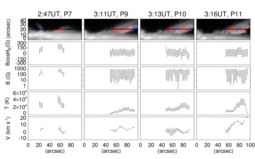
Figure 6: Inverted magnetic field, temperature, and Doppler velocity for the observed jets and surge at the position of the slit shown in the figure. The columns, from left to right, show the inversion results for the observed Stokes spectra of P7 (2:47 UT), P9 (3:11 UT), P10 (3:13 UT), and P11 (3:16 UT). The slit-jaw images in the top row show the direction of the magnetic field on the POS. The red lines indicate inverted solutions affected by the $90^{\circ}$ azimuthal ambiguity, while the blue lines correspond to the solutions with nonambiguous azimuth. The second to fifth rows show, respectively, the longitudinal component of the magnetic field, the magnetic field strength, the temperature, and the Doppler velocity. The abscissas indicate the position along the slit.

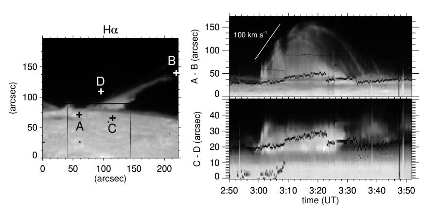
Figure 7: Left: Slit-jaw image in H$\alpha$ of the surge observed at 3:16 UT. Right: Time-distance diagrams obtained between the points A and B (top), and C and D (bottom), marked on the slit-jaw image on the left. The thick dots in the diagrams show the spectrograph slit. The thin dots in the top diagram show one of the spectrograph hairlines.

References

- Anan et al. (2012) Anan, T., Ichimoto, K., Oi, A., Kimura, G., Nakatani, Y., & Ueno, S. 2012, Proc. SPIE, 8446, 46
- Berger et al. (2008) Berger, T. E., et al. 2008, ApJ, 676, 89
- Bommier et al. (1986) Bommier, V., Leroy, J. L., & Sahal-Brchot, S. 1986, A&A, 156, 90
- Casini & Landi Degl’Innocenti (1993) Casini, R., & Landi Degl’Innocenti, E. 1993, A&A, 276, 289
- Casini & Foukal (1996) Casini, R., & Foukal, P. 1996, Sol. Phys., 163, 65
- Casini & Judge (1999) Casini, R., & Judge, P. G. 1999, ApJ, 522, 524
- Casini (2002) Casini, R. 2002, ApJ, 568, 1056
- Casini et al. (2003) Casini, R., Lpez Ariste, Tomczyk, S., & Lites, B., W. 2003, ApJ, 598, 67
- Casini et al. (2005) Casini, R., Bevilacqua, R., & Lpez Ariste, A. 2005, ApJ, 622, 1265
- Casini (2005) Casini, R. 2005, PhRvA, 71, 2505
- Casini & Manso Sainz (2006) Casini, R. & Manso Sainz, R. 2006, JPhB, 39, 3241
- Casini et al. (2009) Casini, R., Lpez Ariste, A., Paletou, F., & Lger, L. 2009, ApJ, 703, 114
- Collados et al. (2007) Collados, M., Lagg, A., Garc, A., J., J., Surez, E., H., Lpez, R., L., Ma, E., P., & Solanki, S., K. 2007, PASP, 368, 611
- Favati et al. (1987) Favati, B., Landi Degl’Innocenti, E., & Landolfi, M. 1987, A&A, 179, 329
- Foukal & Hinata (1991) Foukal, P., & Hinata, S. 1991, Sol. Phys., 132, 307
- Foukal & Behr (1995) Foukal, P., & Behr, B. 1995, Sol. Phys., 156, 293
- Gaizauskas (1996) Gaizauskas, V. 1996, Sol. Phys., 169, 357
- Gary (2001) Gary, G., A. 2001, Sol. Phys., 203, 71
- Gilbert et al. (2002) Gilbert, H. R., Hansteen, V., H., & Holzer, T. E. 2002, ApJ, 577, 464
- Goto (2008) Goto, M. 2008, Plasma Polarization Spectroscopy ed. Fujimoto, T & Iwamae, A., chapter 2
- House (1977) House, L. L. 1977, ApJ, 214, 632
- Ichimoto et al. (2008) Ichimoto, K., et al. 2008, Sol. Phys., 249, 233
- Illing (1974) Illing, R. M. E., Landman, D. A. & Mickey, D. L. 1974, A&A, 35, 327
- Jaeggli et al. (2010) Jaeggli, S., A., Lin, H., Mickey, D., L., Kuhn, J., R., Hegwer, S., L, Rimmele, T., R., & Penn, M., J. 2010, Memorie della Societa Astronomica Italiana, 81, 763
- Katsukawa et al. (2007) Katsukawa, Y., Berger, T. E., Ichimoto, K., Lites, B. W., Nagata, S., Shimizu, T., Shine, R. A., Suematsu, Y., Tarbell, T. D., Title, A. M., & Tsuneta, S. 2007, Sci., 318, 1594
- Kemp et al. (1984) Kemp, J. C., Macek, J. H., & Nehring F. W. 1984, ApJ, 278, 863
- Kramida (2010) Kramida, A., E. 2010, Atomic Data and Nuclear Data Tables, 96, 586
- Kurokawa (1988) Kurokawa, H. 1988, Vistas in Astronomy, 31, 67
- Kurucz et al. (1984) Kurucz, R. L., Furenlid, I., Brault, J., & Testerman, L. 1984, sfat.book
- Lagg et al. (2004) Lagg, A., Woch, J., Krupp, N., & Solanki, S., K. 2004, A&A, 414, 1109
- Landi Degl’Innocenti (1982) Landi Degl’Innocenti, E., Sol. Phys., 79, 291
- Landi Degl’Innocenti & Landolfi (2004) Landi Degl’Innocenti, M., & Landolfi, M. 2004, Polarization in Spectral Lines
- Lehmann (1964) Lehmann, J. H. 1964, J. Phys., 25, 809
- Lpez Ariste & Casini (2002) Lpez Ariste, A., & Casini, R. 2002, ApJ, 575, 529
- Lpez Ariste & Casini (2005) Lpez Ariste, A., & Casini, R. 2005, A&A, 436, 325
- Merenda et al. (2006) Merenda, L., Trujillo Bueno, J., Landi Degl’Innocenti, E., & Collados, M. 2006, ApJ, 642, 554
- Moran & Foukal (1991) Moran, T., & Foukal, P. 1991, Sol. Phys., 135, 179
- Morita et al. (2010) Morita, S., Shibata, K., Ueno, S., Ichimoto, K., Kitai, R., & Otsuji, K. 2010, PASJ, 62, 901
- Nakai & Hattori (1985) Nakai, Y., & Hattori, A. 1985, Memoirs of the Faculty of Science, Kyoto University, 36, 385
- Nakamura et al. (2012) Nakamura, N., Shibata, K., & Isobe, H. 2012, ApJ, 761, 87
- Nishizuka et al. (2008) Nishizuka, N., Shimizu, M., Nakamura, T., Otsuji, K., Okamoto, T. J., Katsukawa, Y., & Shibata, K. 2008, ApJ, 683, 83
- Nishizuka et al. (2011) Nishizuka, N., Nakamura, T., Kawate, T., Singh, K., A., P., & Shibata, K. 2011, ApJ, 731, 43
- Rees et al. (2000) Rees, D. E., Lpez Ariste, A., Thatcher, J., & Semel, M, 2000, A&A, 335, 759
- Roy (1973) Roy, V., -R. 1973, Sol. Phys., 28, 95
- Rust (1968) Rust, D., M. 1968, in proceedings of the International Astronomical Union Sympossium, 35, 77
- Ryutova et al. (2008) Ryutova, M., Berger, T., Frank, Z., & Title, A. 2008, ApJ, 686, 1404
- Sahal-Brchot et al. (1996) Sahal-Brchot, S., Vogt, E., Thoraval, S., & Diedhiou, I. 1996, A&A, 309, 317
- Sasso et al. (2011) Sasso, C., Lagg, A., & Solanki, S. K. 2011, A&A, 526, A42
- Shibata et al. (2007) Shibata, K., et al. 2007, Science, 318, 1591
- Socas-Navarro et al. (2001) Socas-Navarro, H., Lpez Ariste, A., & Lites, B. W. 2001, ApJ, 553, 949
- & Trujillo Bueno (2011) , J., & Trujillo Bueno, J. 2011, ApJ, 732, 80
- Takasao et al. (2013) Takasao, S., Isobe, H., & Shibata, K. 2013, PASJ, 65, 62
- Trujillo Bueno et al. (2002) Trujillo Bueno, J., Landi Degl’Innocenti, E., Collados, M., & Manso Sainz, R. 2002, Nature, 415, 403
- Trujillo Bueno et al. (2005) Trujillo Bueno, J., Merenda, L., Centeno, R., Collados, M., & Landi Degl’Innocenti, E. 2005, ApJ, 619, 191
- Trujillo Bueno & Asensio Ramos (2007) Trujillo Bueno, J., & Asensio Ramos, A. 2007, ApJ, 655, 642
- Vernazza et al. (1981) Vernazza, J. E., Avrett, E. H., & Loeser, ApJS, 45, 635
- Zirker et al. (1998) Zirker, J. B., Engvold, O., & Martin, S. F. 1998, Nature, 396, 440