Sub-Modularity of Waterfilling with Applications to Online Basestation Allocation

Abstract

We show that the popular water-filling algorithm for maximizing the mutual information in parallel Gaussian channels is sub-modular. The sub-modularity of water-filling algorithm is then used to derive online basestation allocation algorithms, where mobile users are assigned to one of many possible basestations immediately and irrevocably upon arrival without knowing the future user information. The goal of the allocation is to maximize the sum-rate of the system under power allocation at each basestation. We present online algorithms with competitive ratio of at most 2 when compared to offline algorithms that have knowledge of all future user arrivals.

I Introduction

In combinatorial optimization, sub-modular functions play the role of convex functions in continuous optimization. For a sub-modular function, the incremental gain from adding an extra element in the set decreases with the size of the set. The interest in sub-modular functions is because results in combinatorial optimization show that greedy algorithms are close to optimal algorithms with provable guarantees [1, 2].

In this paper, we show that the water-filling algorithm for maximizing the mutual information in parallel Gaussian channels is sub-modular. Log-based utility functions arising from the capacity of a Gaussian channel are used in resource allocation for which water-filling is the optimal solution. Thus, the sub-modularity of water-filling has widespread applications in combinatorial resource allocation. We present one example on online basestation allocation of mobile users to basestations with $\log$-utility based power allocation.

Specifically, we consider the online downlink basestation association problem, where each user on its arrival reveals its SNRs to each of the basestations, and is allocated to one of the basestations for maximizing the sum-rate at the end of all user arrivals. Each user is allocated immediately upon arrival, and the association once made cannot be revoked.

An online algorithm allocates users causally without information about future user arrivals. On the other hand, in an offline algorithm, all future user arrivals and rates are revealed in the beginning. The performance of an online algorithm is characterized by its competitive ratio, which is the ratio of the utility of the offline algorithm to that of the online algorithm [3]. The problem is then to find online algorithms with smallest possible competitive ratio.

Associating mobile users to basestations under different utility models is a classical problem in the literature. Many utility models have been considered in prior work including load balancing [4, 5, 6], cell breathing [7], call admission [8] and fairness [9], sub-carrier/power allocation either jointly with base-station allocation [10] or without it [11][12]. Most of the prior work on allocation assumes either exact user information or statistics is known and formulates a joint optimization problem. In contrast, design and analysis of online algorithms for the basestation association problem do not require any information or assumption about the statistics of the user’s profile.

Online algorithms have been designed for many related problems in literature, e.g., load balancing [13], load balancing with deadlines [14], maximum weight matching [15], picking best subset of fixed cardinality [16] (called the $k$-secretary problem), and multi-partitioning [1, 2]. Our contributions are as follows:

• We prove that the water-filling function that corresponds to maximizing the mutual information of parallel Gaussian channel under a sum-power constraint is sub-modular. To the best of our knowledge, the sub modularity of the waterfilling algorithm is not known in literature, and is an important result with several ramifications in combinatorial resource allocation.

• We exploit the sub-modularity of the water-filling function to derive a $2$-competitive online basestation allocation algorithm for any input (possibly chosen by an adversary) by using results from [1, 2].

II Sub-Modularity of the Waterfilling Function

Consider $M$ parallel Gaussian channels

$$Y_{i}=X_{i}+Z_{i},\ \ \ i=1,2,\ldots,M,$$

with noise variance ${\mathbb{E}}\{Z_{i}^{2}\}=N_{i}>0$, and sum-power constraint ${\mathbb{E}}\{\sum_{i=1}^{M}X_{i}^{2}\}\leq P$. To maximize the mutual information between the input and the output over a subset of channels $S\subseteq\{1,2,\ldots,M\}$, we have to solve

$$\max\;\; R(S)=\sum_{i\in S}\log\left(1+\frac{P_{i}}{N_{i}}\right)$$ (1)

subject to $$\sum_{i\in S}P_{i}\leq P,\ P_{i}\geq 0,\ i\in S.$$

The optimal solution to (1) is given by $P^{*}_{i}=(\nu(S)-N_{i})^{+}$, and $\nu(S)$ is the so-called water level $\nu$ chosen to satisfy

$$\sum_{i\in S}(v(S)-N_{i})^{+}=P,$$ (2)

with $(x)^{+}=x$, for $x>0$ and $0$ otherwise, and the optimal objective function is

$$R^{*}(S)=\sum_{i\in S}\log\left(1+\frac{(\nu(S)-N_{i})^{+}}{N_{i}}\right).$$ (3)

The optimal power allocation $P^{*}$ is popularly known as the waterfilling, and we call $R^{*}(S)$ as the waterfilling function. Note that $R^{*}(S)$ is a set function from the power set of $\{1,2,\ldots,M\}$ to the real numbers. Also note that,

$$R^{*}(S)=\sum_{i\in S:\nu(S)>N_{i}}\log\left(\frac{\nu(S)}{N_{i}}\right)=\log\frac{\nu(S)^{|T(S)|}}{\prod_{i\in T(S)}N_{i}},$$ (4)

where

$$T(S)=\{i\in S:\nu(S)>N_{i}\},$$ (5)

denotes the channels in $S$ that are allotted non-zero power. Using the definition of $T(S)$ in (2), we get that

$$\sum_{i\in T(S)}(v(S)-N_{i})=|T(S)|\nu(S)-\sum_{i\in T(S)}N_{i}=P.$$ (6)

Definition 1.

Let $U$ be a finite set, and let $2^{U}$ be the power set of $U$. A real-valued set function $f:2^{U}\to\mathbb{R}$ is said to be monotone if $f(S)\leq f(T)$ for $S\subseteq T\subseteq U$, and submodular if

$$f(S)+f(T)\geq f(S\cap T)+f(S\cup T),\ \forall S,T\in 2^{U}.$$ (7)

An equivalent definition of sub-modularity is

$$f(S\cup\{i\})+f(S\cup\{j\})\geq f(S)+f(S\cup\{i,j\})$$ (8)

for every $S\subseteq U$ and every $i,j\in U\setminus S$ with $i\neq j$.

Theorem 2.

Water-filling function $R^{*}(\cdot)$ is sub-modular.

Proof.

We will show the sub-modularity of $R^{*}(\cdot)$ by showing that $R^{*}(\cdot)$ satisfies (8). There are four different waterfilling function evaluations in (8), that involve the following four water levels $\nu_{i}=\nu(S\cup\{i\})$, $\nu_{j}=\nu(S\cup\{j\})$, $\nu=\nu(S)$, and $\nu_{ij}=\nu(S\cup\{i,j\})$, respectively.

Figure 1: Illustration of water levels, $S=\{1,2,3,4,5,6\}$.

As illustrated in Fig. 1, we have the following relationships among the water levels:

$$\nu_{ij}\leq\nu_{i}\leq\nu,\ \nu_{ij}\leq\nu_{j}\leq\nu.$$ (9)

Without loss of generality, we assume that $\nu_{j}\geq\nu_{i}$. So, we have

$$\nu_{ij}\leq\nu_{i}\leq\nu_{j}\leq\nu.$$ (10)

Similarily, let the channels receiving non-zero power be $T=T(S)$, $T_{i}=T(S\cup\{i\})$, $T_{j}=T(S\cup\{j\})$ and $T_{ij}=T(S\cup\{i,j\})$. Finally, let the optimal rates be $R^{*}=R^{*}(S)$, $R^{*}_{i}=R^{*}(S\cup\{i\})$, $R^{*}_{j}=R^{*}(S\cup\{j\})$ and $R^{*}_{ij}=R^{*}(S\cup\{i,j\})$.

Also, the optimal rates satisfy the following relationship:

$$R^{*}_{ij}\geq R^{*}_{i}\geq R^{*},\ R^{*}_{ij}\geq R^{*}_{j}\geq R^{*}.$$ (11)

Using the above relationships, we first settle two easy cases. If $i\notin T_{ij}$, then $R^{*}_{ij}=R^{*}_{j}$, and the submodularity condition (8) is seen to be readily satisfied using (11). By a similar argument, if $j\notin T_{ij}$, then $R^{*}_{ij}=R^{*}_{i}$ and hence (8) is clearly satisfied.

So, in what follows, we will assume that $i,j\in T_{ij}$. If $i,j\in T_{ij}$, we have $\nu_{ij}>N_{i}$ and $\nu_{ij}>N_{j}$, which, by (9), results in $\nu_{i}>N_{i}$ and $\nu_{j}>N_{j}$. This implies that $i\in T_{i}$ and $j\in T_{j}$. Now, let $\bar{T}_{ij}=T_{ij}\setminus\{i,j\}$, $\bar{T}_{i}=T_{i}\setminus\{i\}$ and $\bar{T}_{j}=T_{j}\setminus\{j\}$. From (9), it is clear that $\bar{T}_{ij}\subseteq\bar{T}_{i}$ and $\bar{T}_{j}\subseteq T$. Further, letting $\hat{T}_{i}=\bar{T}_{i}\setminus\bar{T}_{ij}$ and $\hat{T}=T\setminus\bar{T}_{j}$, we can write

$$T_{i}=\{i\}\sqcup\bar{T}_{ij}\sqcup\hat{T}_{i},\ T_{j}=\{j\}\sqcup\bar{T}_{j},$$ (12)

$$T=\bar{T}_{j}\sqcup\hat{T},\ \ \ \ \ T_{ij}=\{i,j\}\sqcup\bar{T}_{ij},$$ (13)

where $\sqcup$ denotes disjoint union.

After a series of simplifications shown in Appendix A, we reduce the condition for submodularity of $R^{*}$ to the following:

$$\nu_{i}^{|T_{i}|}\ \nu_{j}^{|T_{j}|}\ \prod_{l\in\hat{T}}N_{l}\geq\nu^{|T|}\ \nu_{ij}^{|T_{ij}|}\ \prod_{m\in\hat{T}_{i}}N_{m}.$$ (14)

The terms involved in (14) can be ordered in a specific way, and this is stated in the next Lemma:

Lemma 3.

The following ordering holds true for every $m\in\hat{T}_{i}$ and every $l\in\hat{T}$:

$$\nu_{ij}\overset{(a)}{\leq}N_{m}\overset{(b)}{\leq}\nu_{i}\overset{(c)}{\leq}\nu_{j}\overset{(d)}{\leq}N_{l}\overset{(e)}{\leq}\nu.$$ (15)

Proof.

See Appendix B. ∎

In particular, by Lemma 3, all terms in the LHS of (14) are bounded between two terms $N_{m^{*}}$ and $\nu$ in the RHS, where $m^{*}=\arg\max_{m\in\hat{T}_{i}}N_{m}$, is the highest noise level in $\hat{T}_{i}$. This is a crucial observation, and is exploited later. The next Lemma states two equalities on the terms involved in (14).

Lemma 4.

The following relationships hold true:

$$|T_{i}|\nu_{i}+|T_{j}|\nu_{j}+\sum_{l\in\hat{T}}N_{l} =|T|\nu+|T_{ij}|\nu_{ij}+\sum_{m\in\hat{T}_{i}}N_{m},$$ (16)

$$|T_{i}|+|T_{j}|+|\hat{T}| =|T|+|T_{ij}|+|\hat{T}_{i}|.$$ (17)

Proof.

See Appendix C. ∎

In words, Lemma 4 states that the number of terms and their sum in the LHS and RHS of (14), counting multiplicities, are equal. The next Lemma is a general version of the inequality in (14) with constraints motivated by Lemmas 3 and 4.

Lemma 5.

Let $a_{i}$, $b_{i}$, $1\leq i\leq n$, be positive real numbers with $a_{1}\leq a_{2}\leq\ldots\leq a_{n}$, $b_{1}\leq b_{2}\leq\ldots\leq b_{n}$, and

$$\sum^{n}_{i=1}a_{i}=\sum^{n}_{j=1}b_{j}.$$ (18)

If $\exists$ $k$, $1\leq k\leq n-1$, for which

$$a_{k}\leq b_{1}\leq b_{2}\leq\ldots\leq b_{n}\leq a_{k+1},$$ (19)

then, we have,

$$\prod^{n}_{j=1}b_{j}\geq\prod^{n}_{i=1}a_{i}.$$ (20)

Proof.

See Appendix D. ∎

To show the sub-modularity of $R^{*}$, i.e. to prove (14), we use Lemma 20 with suitable choices for $a_{i}$, $b_{i}$. Let ${\mathbf{a}}=[a_{n}\ a_{n-1}\ \cdots\ a_{1}]$ be defined as follows:

$${\mathbf{a}}=[\underbrace{\cdots\ \nu\ \cdots}_{|T|\text{ times}}\ \underbrace{\cdots\ N_{m}\ \cdots}_{m\in\hat{T}_{i}}\ \underbrace{\cdots\ \nu_{ij}\ \cdots}_{|T_{ij}|\text{ times}}],$$ (21)

where the numbers in the set $\{N_{m}:m\in\hat{T}_{i}\}$ are arranged in non-increasing order. Similarly, the vector ${\mathbf{b}}=[b_{n}\ b_{n-1}\ \cdots\ b_{1}]$ is defined to be

$${\mathbf{b}}=[\underbrace{\cdots\ N_{l}\ \cdots}_{l\in\hat{T}}\ \underbrace{\cdots\ \nu_{j}\ \cdots}_{|T_{j}|\text{ times}}\ \underbrace{\cdots\ \nu_{i}\ \cdots}_{|T_{i}|\text{ times}}],$$ (22)

where, once again, the numbers in the set $\{N_{l}:l\in\hat{T}\}$ are arranged in non-increasing order. Firstly, ${\mathbf{a}}$ and ${\mathbf{b}}$ defined above have the same length by (17) in Lemma 4. Further, by Lemmas 3 and 4, ${\mathbf{a}}$ and ${\mathbf{b}}$ satisfy the constraints (18), (19) of Lemma 20. Hence, by the result of Lemma 20, we have

$$\prod^{n}_{j=1}b_{j}=\nu_{i}^{|T_{i}|}\ \nu_{j}^{|T_{j}|}\ \prod_{l\in\hat{T}}N_{l}\geq\prod^{n}_{i=1}a_{i}=\nu^{|T|}\ \nu_{ij}^{|T_{ij}|}\ \prod_{m\in\hat{T}_{i}}N_{m}.$$

∎

Next, we present an important problem of online basestation allocation, where we use the sub-modularity of water-filling to show that the sum-rate obtained by a greedy online algorithm is no less than $2$ times that of an optimal offline algorithm.

III Online Basestation Allocation

Consider the scenario where $n$ mobile users arrive one at a time into a geographical area with $m$ basestations with $m<n$. User $i$ has a non-negative weight $w_{ij}$ to basestation $j$, which is the signal-to-noise ratio (SNR) of the user’s channel to the basestation. The weights $w_{ij}$ are collected into an $n\times m$ matrix $W$ for easy reference.

In the downlink basestation allocation problem, each user is to be allotted to exactly one of the $m$ basestations. An arbitrary allocation is specified by the family of sets $\mathcal{M}=\{M_{j}:1\leq j\leq m\}$, where $M_{j}$ is the set of users allotted to basestation $j$. Note that the sets $M_{j}$ partitions the set of users. The goal is to maximize a utility function over the allocations $\mathcal{M}$.

We will enforce two important conditions on the allocation policy: (1) each user needs to be allotted to a basestation immediately upon arrival, and (2) this allocation is irrevocable and cannot be altered subsequently.

III-A Offline versus online allocation

In an offline allocation problem, the entire weight matrix $W$ is available ahead of time. So, an offline algorithm solves a well-defined optimization of the utility over all possible allocations. Let us denote the optimal offline utility by $R^{*}_{\text{off}}(W)$.

In an online allocation problem, the users arrive in an arbitrary order, and weights of user $i$ are revealed only upon arrival. i.e. the $i$-th row of $W$ is revealed when user $i$ arrives.

Online algorithms are, by definition, poorer than offline algorithms. Competitive ratio is a popular figure of merit used to characterize and compare online and offline algorithms [3]. For a given weight matrix $W$, the competitive ratio of an online algorithm $\mathcal{A}$ is defined as $\eta_{W}(\mathcal{A})=R^{*}_{\text{off}}(W)/R_{\mathcal{A}}(W)$, where $R_{\mathcal{A}}(W)$ denotes the utility of the online algorithm $\mathcal{A}$ on input $W$. Since $R^{*}_{\text{off}}(W)\geq R_{\mathcal{A}}(W)$, we have $\eta_{W}(\mathcal{A})\geq 1$ for all $W$ and $\mathcal{A}$. The worst-case competitive ratio of an online algorithm $\mathcal{A}$ is defined as $\eta_{\text{worst}}(\mathcal{A})=\max_{W}\eta_{W}(\mathcal{A})$. The design goal is to have online algorithms with a competitive ratio as close to 1 as possible.

III-B Utility and greedy online algorithm

We suppose that each basestation has unit transmit power that is allocated to each of its connected users such that it maximizes the $\log$-utility. Thus, to maximize the rate, basestation $j$ allocates power $\alpha_{ij}$ to all its connected users $i\in M_{j}$ by performing the following maximization:

$$L(M_{j})=\max_{\alpha_{ij},\sum_{i\in M_{j}}\alpha_{ij}\leq 1}\sum_{i\in M_{j}}\log(1+\alpha_{ij}w_{ij}),$$ (23)

where the weight $w_{ij}$ is the channel SNR of user $i$ to basestation $j$. We consider the online basestation allocation problem, where each user on its arrival is assigned to one of the base stations, i.e. to one of sets $M_{j},j=1,\dots,m$ without knowing any information about the future user arrivals, so as to maximize the overall utility

$$LS(\mathcal{M},W)=\sum_{j=1}^{m}L(M_{j}),$$ (24)

which is the sum rate of the entire system over all basestations.

We propose an online algorithm for basestation allocation that maximizes the sum-rate (24) at a worst-case competitive ratio of at most $2$. The algorithm and proof use results on the multi-partitioning problem in [1, 2].

Definition 6.

Multi-partitioning problem: The problem is to partition a given set ${\mathbf{S}}$ into $k$ subsets $S_{1},\dots,S_{k},S_{i}\cap S_{j}=\phi,\cup_{i=1}^{k}S_{i}={\mathbf{S}}$ such that $\sum_{i=1}^{k}f_{i}(S_{i})$ is maximized.

	ONLINE GREEDY ALLOCATION
1	Initialize $S_{j}=\Phi$, $j=1,\ldots,k$, $i=1$.
2	Find $j^{*}=\arg\max_{j}f_{j}(S_{j}\cup\{i\})$.
3	Update $S_{j^{*}}=S_{j^{*}}\cup\{i\}$.
4	Set $i=i+1$, Stop if $i>|{\mathbf{S}}|$, otherwise go to step 2.
5	Return $S_{j}$, $j=1,\dots,k$.

Theorem 7 ([1, 2]).

If all functions $f_{i}$ in the multi-partitioning problem are non-negative, monotone and sub-modular, then the ONLINE GREEDY ALLOCATION algorithm (presented above) has a competitive ratio of at most $2$.

Note that the sum-rate maximization problem (24) can be thought of as a multi-partioning problem, where $f_{j}=L(M_{j})$. To make use of Theorem 7, we need to check that the function $L(M_{j})$ is sub-modular. Now, note that (23) is a special case of the water-filling function (1), where $P_{i}$ plays the role of $\alpha_{ij}$, sum-power constraint $P=1$, and $w_{ij}=\frac{1}{N_{i}}$. Also, note that (23) is non-negative and monotone. Therefore, we have the following:

Theorem 8.

The competitive ratio of the ONLINE GREEDY ALLOCATION algorithm is $\leq 2$ for maximizing the sum-rate (24).

Proof.

Follows from Theorem 7, and Theorem 2, where $|{\mathbf{S}}|=n$, $S_{j}=M_{j}$, $j=1,\dots,m$, and $f_{j}=L(M_{j})$ for the ONLINE GREEDY ALLOCATION algorithm. ∎

IV Simulation Results

In Fig. 2, we plot an upper bound on the competitive ratio for the GREEDY ALLOCATION algorithm with $m=10$ basestations under different user SNR profiles. To upper bound the competitive ratio, we upper bound the utility of the offline algorithm by assuming that each user has all SNRs equal to maximum SNR across all the users and all the basestations. Under this assumption, allocating equal number of users to each basestation is optimal. First, we consider the i.i.d. case, where each user’s SNR is distributed uniformly in either $[0,1]$ or $[0,10]$ to all the basestations. We see that in both the cases the competitive ratio upper bound is very close to $1$, which is significantly better than the derived worst case bound of $2$.

Next, we consider two non-i.i.d. cases for the user SNRs – case $1$, where all the SNRs of half of the users are uniformly distributed in $[0,10]$, while the SNRs of the other half of the users are uniformly distributed in $[0,5]$; and case $2$, where for each user, SNRs to 3 randomly selected basestations are uniform in $[0,10]$ and other SNRs are uniform in $[0,1]$. This creates users SNRs with different orders of magnitude. Here also the competitive ratios are very close to unity.

Finally, we consider a case of correlated user SNRs, where for each user 3 randomly selected basestations have the same SNR values while the other basestations have half that value. We see that even for this highly correlated case, competitive ratio is below the stipulated value of $2$, which clearly validates Theorem 8.

For comparison we also plot the competitive ratios of MAX-WEIGHT strategy, which assigns users to the basestation to which it has the highest SNR, for the i.i.d. case 1 and the correlated case. In the former the competitive ratios are the same for both the algorithms, but in the latter, GREEDY algorithm performs significantly better than the MAX-WEIGHT strategy.

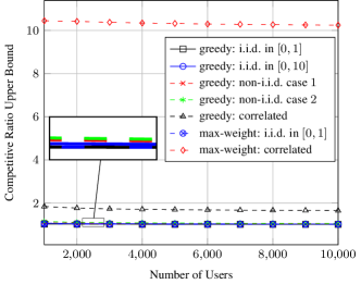
Figure 2: Competitive ratio of different algorithms with $m=10$ basestations.

Appendix A

Using (4), in order for the submodularity condition (8) to be true, we need to show that

$$\log\frac{\nu_{i}^{|T_{i}|}}{\prod_{k\in T_{i}}N_{k}}+\log\frac{\nu_{j}^{|T_{j}|}}{\prod_{k\in T_{j}}N_{k}}\geq\log\frac{\nu^{|T|}}{\prod_{k\in T}N_{k}}+\log\frac{\nu_{ij}^{|T_{ij}|}}{\prod_{k\in T_{ij}}N_{k}},$$

which simplifies to

$$\frac{\nu_{i}^{|T_{i}|}}{\prod_{k\in T_{i}}N_{k}}\ \frac{\nu_{j}^{|T_{j}|}}{\prod_{k\in T_{j}}N_{k}}\geq\frac{\nu^{|T|}}{\prod_{k\in T}N_{k}}\ \frac{\nu_{ij}^{|T_{ij}|}}{\prod_{k\in T_{ij}}N_{k}}.$$ (25)

Using the decompositions in (12) - (13) for the products in the denominator of (25), we get

$$\frac{\nu_{i}^{|T_{i}|}}{N_{i}\prod_{k\in\bar{T}_{ij}}N_{k}\prod_{m\in\hat{T}_{i}}N_{m}}\ \frac{\nu_{j}^{|T_{j}|}}{N_{j}\prod_{k\in\bar{T}_{j}}N_{k}}$$

$$\geq\frac{\nu^{|T|}}{\prod_{k\in\bar{T}_{j}}N_{k}\prod_{l\in\hat{T}}N_{l}}\ \frac{\nu_{ij}^{|T_{ij}|}}{N_{i}N_{j}\prod_{k\in\bar{T}_{ij}}N_{k}},$$

which simplifies to (14), after canceling $N_{i}N_{j}\prod_{k\in\bar{T}_{ij}}N_{k}\prod_{k\in\bar{T}_{j}}N_{k}$ and cross multiplication.

Appendix B Proof of Lemma 3

We use the definition of the set $T(\cdot)$ in (5). Since $m\in\hat{T}_{i}=\bar{T}_{i}\setminus\bar{T}_{ij}$, we have that $m\in T_{i}$, but $m\notin T_{ij}$. So, clearly, $N_{m}\leq\nu_{i}$ and $\nu_{ij}\leq N_{m}$. This proves the inequalities $(a)$ and $(b)$. The inequality $(c)$ follows by the assumption in (10).

Since $l\in\hat{T}=T\setminus\bar{T}_{j}$, we have that $l\in T$, but $l\notin T_{j}$. So, clearly, $N_{l}\leq\nu$ and $\nu_{j}\leq N_{l}$. This proves the final two inequalities $(d)$ and $(e)$.

Appendix C Proof of Lemma 4

Using (6), we have

$$|T_{i}|\nu_{i}=P+\sum_{k\in T_{i}}N_{k},\ \ |T_{j}|\nu_{j}=P+\sum_{k\in T_{j}}N_{k},$$ (26)

$$|T|\nu=P+\sum_{k\in T}N_{k},\ \ |T_{ij}|\nu_{ij}=P+\sum_{k\in T_{ij}}N_{k}.$$ (27)

From (26) and (27), we have

$$|T_{i}|\nu_{i}+|T_{j}|\nu_{j}+\sum_{l\in\hat{T}}N_{l}=2P+\sum_{k\in T_{i}}N_{k}+\sum_{k\in T_{j}}N_{k}+\sum_{l\in\hat{T}}N_{l}.$$ (28)

Using the decompositions for $T_{i}$ and $T_{j}$ in (12), we have

$$\sum_{k\in T_{i}}N_{k} =N_{i}+\sum_{k\in\bar{T}_{ij}}N_{k}+\sum_{m\in\hat{T}_{i}}N_{m},$$ (29)

$$\sum_{k\in T_{j}}N_{k} =N_{j}+\sum_{k\in\bar{T}_{j}}N_{k}.$$ (30)

Using (29), (30) in the RHS of (28) and rearranging, we get

$$|T_{i}|\nu_{i}+|T_{j}|\nu_{j}+ \sum_{l\in\hat{T}}N_{l}=P+\sum_{k\in\bar{T}_{j}}N_{k}+\sum_{l\in\hat{T}}N_{l}+$$

$$P+N_{i}+N_{j}+\sum_{k\in\bar{T}_{ij}}N_{k}+\sum_{m\in\hat{T}_{i}}N_{m}.$$ (31)

Using (13) and (27), the RHS of (31) and (16) are seen to be equal, proving (16). To prove (17), we use (12) to get

$$|T_{i}|+|T_{j}|+|\hat{T}| =1+|\bar{T}_{ij}|+|\hat{T}_{i}|+1+|\bar{T}_{j}|+|\hat{T}|,$$

$$=(|\bar{T}_{j}|+|\hat{T}|)+(2+|\bar{T}_{ij}|)+|\hat{T}_{i}|,$$

$$=|T|+|T_{ij}|+|\hat{T}_{i}|.$$ (32)

Appendix D Proof of Lemma 20

The first step in the proof is to show that the conditions on $a_{i}$, $b_{j}$ imply that the vector $[a_{n}\ a_{n-1}\ \cdots\ a_{1}]$ majorizes the vector $[b_{n}\ b_{n-1}\ \cdots\ b_{1}]$. Since the sum of the two vectors are equal (from (18)), we only need to show, for $1\leq i\leq n$,

$$A_{i}\triangleq a_{n}+a_{n-1}+\cdots+a_{i}\geq B_{i}\triangleq b_{n}+b_{n-1}+\cdots+b_{i}.$$ (33)

From (19), it is clear that $A_{i}\geq B_{i}$ for $k+1\leq i\leq n$. For $1\leq i\leq k$, we have $a_{i}\leq b_{i}$, or

$$A_{i}-A_{i+1}\leq B_{i}-B_{i+1}.$$ (34)

Summing (34) from $i-1$ down to $i=1$, we get

$$A_{1}-A_{i}\leq B_{1}-B_{i},\ 1\leq i\leq k.$$ (35)

Since $A_{1}=B_{1}$, we have $A_{i}\geq B_{i}$, $1\leq i\leq k$. This proves that $[a_{n}\ a_{n-1}\ \cdots\ a_{1}]$ majorizes $[b_{n}\ b_{n-1}\ \cdots\ b_{1}]$.

The second step is to invoke Karamata’s inequality [17][18], which states that

$$g(a_{1})+g(a_{2})+\cdots+g(a_{n})\geq g(b_{1})+g(b_{2})+\cdots+g(b_{n}),$$ (36)

for any convex function $g$, if $[a_{n}\ a_{n-1}\ \cdots\ a_{1}]$ majorizes $[b_{n}\ b_{n-1}\ \cdots\ b_{1}]$. Using (36) with $g(\cdot)=-\log(\cdot)$, the claim of the Lemma in (20) follows.

References

• [1] M. L. Fisher, G. L. Nemhauser, and L. A. Wolsey, “An analysis of approximations for maximizing submodular set functions - II,” Mathematical Programming, vol. 14, no. 1, pp. 265–294, Dec. 1978.
• [2] B. Lehmann, D. Lehmann, and N. Nisan, “Combinatorial auctions with decreasing marginal utilities,” Games and Economic Behavior, vol. 55, no. 2, pp. 270–296, 2006.
• [3] A. Borodin and R. El-Yaniv, Online Computation and Competitive Analysis.   Cambridge University Press, 1998.
• [4] K. Son, S. Chong, and G. De Veciana, “Dynamic association for load balancing and interference avoidance in multi-cell networks,” IEEE Trans. Wireless Commun., vol. 8, no. 7, pp. 3566–3576, 2009.
• [5] E. Altman, U. Ayesta, and B. J. Prabhu, “Load balancing in processor sharing systems,” Telecommunication Systems, vol. 47, no. 1-2, pp. 35–48, 2011.
• [6] H. Kim, G. De Veciana, X. Yang, and M. Venkatachalam, “Distributed $\alpha$-optimal user association and cell load balancing in wireless networks,” IEEE/ACM Trans. Netw., vol. 20, no. 1, pp. 177–190, 2012.
• [7] Y. Bejerano and H. Seung-Jae, “Cell breathing techniques for load balancing in wireless lans,” IEEE Trans. Mobile Comput., vol. 8, no. 6, pp. 735–749, 2009.
• [8] X. Wu, B. Mukherjee, and S.-H. Chan, “MACA-an efficient channel allocation scheme in cellular networks,” in IEEE Global Telecommunications Conference, 2000. GLOBECOM’00., vol. 3, 2000, pp. 1385–1389.
• [9] Y. Bejerano, S.-J. Han, and L. E. Li, “Fairness and load balancing in wireless lans using association control,” in Proceedings of the 10th ACM Annual International Conference on Mobile Computing and Networking, 2004, pp. 315–329.
• [10] J. Huang, V. G. Subramanian, R. Agrawal, and R. A. Berry, “Downlink scheduling and resource allocation for OFDM systems,” IEEE Trans. Wireless Commun., vol. 8, no. 1, pp. 288–296, 2009.
• [11] K. Kim, Y. Han, and S.-L. Kim, “Joint subcarrier and power allocation in uplink OFDMA systems,” IEEE Commun. Lett., vol. 9, no. 6, pp. 526–528, 2005.
• [12] J. Acharya and R. D. Yates, “Dynamic spectrum allocation for uplink users with heterogeneous utilities,” IEEE Trans. Wireless Commun., vol. 8, no. 3, pp. 1405–1413, 2009.
• [13] Y. Azar, “On-line load balancing,” in Online Algorithms.   Springer, 1998, pp. 178–195.
• [14] S. Moharir, S. Sanghavi, and S. Shakkottai, “Online load balancing under graph constraints,” in Proceedings of the ACM SIGMETRICS/International Conference on Measurement and Modeling of Computer Systems, 2013, pp. 363–364.
• [15] N. Korula and M. Pál, “Algorithms for secretary problems on graphs and hypergraphs,” in Proceedings of the 36th Internatilonal Collogquium on Automata, Languages and Programming: Part II, ser. ICALP ’09.   Berlin, Heidelberg: Springer-Verlag, 2009, pp. 508–520.
• [16] M. Babaioff, N. Immorlica, D. Kempe, and R. Kleinberg, “A knapsack secretary problem with applications,” Approximation, Randomization, and Combinatorial Optimization. Algorithms and Techniques, pp. 16–28, 2007.
• [17] J. Karamata, “Sur une inégalité relative aux fonctions convexes.” Publ. Math. Univ. Belgrade, vol. 1, pp. 145–148, 1932.
• [18] Z. Kadelburg, D. Dukić, M. Lukić, and I. Matić, “Inequalities of Karamata. Schur and Muirhead, and some applications,” The Teaching of Mathematics, vol. 8, no. 1, pp. 31–45, 2005.