Tests for High Dimensional Generalized Linear Models
Song Xi Chen and Bin Guo
Abstract
We consider testing regression coefficients in high dimensional
generalized linear models. An investigation of the test of
Goeman et al. (2011 ) is conducted, which reveals that if the
inverse of the link
function is unbounded,
the high dimensionality in the covariates can impose adverse impacts
on the power of the test. We propose a
test formation which can avoid the
adverse impact of the high dimensionality.
When the inverse of the link function is bounded such as the
logistic or probit regression, the proposed test is as good
as Goeman et al. (2011 ) ’s test.
The proposed tests provide p-values for testing significance for gene-sets as demonstrated in
a case study on an acute lymphoblastic leukemia dataset.
Key words: Generalized Linear Model;
Gene-Sets; High Dimensional Covariates; Nuisance Parameter;
U 𝑈 U
The generalized linear models
(McCullagh and Nelder, 1989 ) are
widely used statistical models in many fields of statistical applications.
The surge of high dimensional data collection and analysis in
bioinformatics and related studies have led to the use of generalized linear models in high dimensional settings. The high dimensionality can
arise at least in two forms. One is in the various multiple response variables but with low or fixed
dimensional covariates where the responses represent the readings
for large number of genes and the covariates represent certain
design and demographic variables. Another is to have low
dimensional response (for instance indicators for a disease) but
high dimensional covariates representing genes expressions levels.
Research works on the first form of high dimensionality
include Auer and Doerge (2010 )
and Lund et al. (2012 ) in the context of next generation sequencing data.
The current paper will be focused on the latter case where the high dimensionality is associated with the covariates.
Statistical inference for the generalized linear models under the high dimensional setting has
been the focus of some latest research. van de Geer (2008 )
considered variable selection via a LASSO approach.
Fan and Song (2010 ) and Chang et al. (2013 ) proposed
approaches via the sure independence screening of
Fan and Lv (2008 ) .
The focus of the paper is on testing for significance of the
regression coefficients of high dimensional generalized linear models, which
is of important interest to practitioners, for instance in the
context of discovering significant gene-sets which is subject to
both high dimensionality and multiplicity as the genes in different gene-sets
can overlap. For fixed dimensional data,
the likelihood ratio test and the Wald
test have been popular choices as elaborated in
McCullagh and Nelder (1989 ) . However, the high dimensionality
renders the applicability of these two tests. There are published
works on testing for the coefficients of high dimensional linear
regression for the large p 𝑝 p n 𝑛 n Zhong and Chen (2011 ) that adapt to the high dimensionality and the factorial designs, and in Lan et al. (2014 ) that allows testing on subsets of the
regression coefficient vector.
Arias-Castro et al. (2011 ) and
Ingster et al. (2010 ) studied the higher
criticism tests (Donoho and Jin, 2004 )
for sparse linear regression models, and demonstrated that the tests can attain the optimal detection boundary for the testing problem.
In an important development,
Goeman et al. (2011 ) proposed tests for the
coefficients of high dimensional generalized linear models in the
presence of nuisance parameters.
The test procedure was formulated by numerically
simulating a ratio of quadratic forms of certain normally
distributed “data” to obtain the critical value. The test of
Goeman et al. (2011 ) allowed the dimension of
the covariates p 𝑝 p n 𝑛 n p 𝑝 p
In this paper, we first analyze the power properties of
Goeman et al. (2011 ) ’s test by allowing p 𝑝 p n 𝑛 n U 𝑈 U Goeman et al. (2011 )
asymptotically. However, when the inverse of the link function is
unbounded, as the case of the log link, the proposed tests have much
better power. These findings are demonstrated by both theoretical
analysis and numerical simulations. We apply the proposed tests in
finding significant gene-sets in an acute lymphoblastic leukemia
dataset. It is shown in the case study that the p-values produced
from the proposed tests when used in conjunction with a proper
control on the False Discovery Rate
(Benjamini and Hochberg, 1995 ) can lead to finding significant gene-sets in the context of high dimensionality and multiplicity.
The paper is organized as follows. In Section 2, we review the
inferential setting for the generalized linear models. Section 3
analyzes Goeman et al. (2011 ) ’s test, which
motivates our proposal for the global test in Section 4 and the test
with nuisance parameters in Section 5.
Results from simulation studies are reported in Section 6. Section 7 presents the case
study on the acute lymphoblastic leukemia dataset. All technical details are relegated to the Appendix.
2. MODELS AND EXISTING TEST
Let Y 𝑌 Y p 𝑝 p X 𝑋 X (McCullagh and Nelder, 1989 )
provide a rich collection of specifications for the conditional mean
of Y 𝑌 Y X 𝑋 X
Conditioning on the covariate X 𝑋 X g ( ⋅ ) 𝑔 ⋅ g(\cdot) V ( ⋅ ) 𝑉 ⋅ V(\cdot)
E ( Y | X ) = μ ( β ) = g ( X T β ) and var ( Y | X ) = V { g ( X T β ) } , formulae-sequence 𝐸 conditional 𝑌 𝑋 𝜇 𝛽 𝑔 superscript 𝑋 T 𝛽 and var conditional 𝑌 𝑋
𝑉 𝑔 superscript 𝑋 T 𝛽 E(Y|X)=\mu(\beta)=g(X^{{\mathrm{\scriptscriptstyle T}}}\beta)\quad\text{and}\quad\text{var}(Y|X)=V\{g(X^{{\mathrm{\scriptscriptstyle T}}}\beta)\}, (2.1)
where
β 𝛽 \beta p 𝑝 p g − 1 ( ⋅ ) superscript 𝑔 1 ⋅ g^{-1}(\cdot)
Let ( X 1 , Y 1 ) , … , ( X n , Y n ) subscript 𝑋 1 subscript 𝑌 1 … subscript 𝑋 𝑛 subscript 𝑌 𝑛
(X_{1},Y_{1}),\ldots,(X_{n},Y_{n}) ( X , Y ) 𝑋 𝑌 (X,Y) 2.1 β 𝛽 \beta
L n ( β ) = ∑ i = 1 n ∫ Y i μ i ( β ) Y i − t V ( t ) 𝑑 t , subscript 𝐿 𝑛 𝛽 superscript subscript 𝑖 1 𝑛 superscript subscript subscript 𝑌 𝑖 subscript 𝜇 𝑖 𝛽 subscript 𝑌 𝑖 𝑡 𝑉 𝑡 differential-d 𝑡 L_{n}(\beta)=\sum_{i=1}^{n}\int_{Y_{i}}^{\mu_{i}(\beta)}\frac{Y_{i}-t}{V(t)}dt, (2.2)
where μ i ( β ) = g ( X i T β ) subscript 𝜇 𝑖 𝛽 𝑔 superscript subscript 𝑋 𝑖 T 𝛽 \mu_{i}(\beta)=g(X_{i}^{{\mathrm{\scriptscriptstyle T}}}\beta) β ^ n subscript ^ 𝛽 𝑛 \hat{\beta}_{n} β 𝛽 \beta
ℓ n ( β ) = ∑ i = 1 n { Y i − g ( X i T β ) } g ′ ( X i T β ) X i V { g ( X i T β ) } = 0 . subscript ℓ 𝑛 𝛽 superscript subscript 𝑖 1 𝑛 subscript 𝑌 𝑖 𝑔 superscript subscript 𝑋 𝑖 T 𝛽 superscript 𝑔 ′ superscript subscript 𝑋 𝑖 T 𝛽 subscript 𝑋 𝑖 𝑉 𝑔 superscript subscript 𝑋 𝑖 T 𝛽 0 \displaystyle\ell_{n}(\beta)=\sum_{i=1}^{n}\frac{\{Y_{i}-g(X_{i}^{{\mathrm{\scriptscriptstyle T}}}\beta)\}g^{\prime}(X_{i}^{{\mathrm{\scriptscriptstyle T}}}\beta)X_{i}}{V\{g(X_{i}^{{\mathrm{\scriptscriptstyle T}}}\beta)\}}=0. (2.3)
The consistency and asymptotic normality of β ^ n subscript ^ 𝛽 𝑛 \hat{\beta}_{n} (McCullagh and Nelder, 1989 ) .
Let β = ( β ( 1 ) T , β ( 2 ) T ) T 𝛽 superscript superscript 𝛽 1 T superscript 𝛽 2 T T \beta=(\beta^{{\mathrm{\scriptscriptstyle(1)}}{\mathrm{\scriptscriptstyle T}}},\beta^{{\mathrm{\scriptscriptstyle(2)}}{\mathrm{\scriptscriptstyle T}}})^{{\mathrm{\scriptscriptstyle T}}} X i = ( X i ( 1 ) T , X i ( 2 ) T ) T subscript 𝑋 𝑖 superscript superscript subscript 𝑋 𝑖 1 T superscript subscript 𝑋 𝑖 2 T T X_{i}=(X_{i}^{{\mathrm{\scriptscriptstyle(1)}}{\mathrm{\scriptscriptstyle T}}},X_{i}^{{\mathrm{\scriptscriptstyle(2)}}{\mathrm{\scriptscriptstyle T}}})^{{\mathrm{\scriptscriptstyle T}}} β ( 1 ) superscript 𝛽 1 \beta^{{\mathrm{\scriptscriptstyle(1)}}} X i ( 1 ) superscript subscript 𝑋 𝑖 1 X_{i}^{{\mathrm{\scriptscriptstyle(1)}}} p 1 subscript 𝑝 1 p_{1} β ( 2 ) superscript 𝛽 2 \beta^{{\mathrm{\scriptscriptstyle(2)}}} X i ( 2 ) superscript subscript 𝑋 𝑖 2 X_{i}^{{\mathrm{\scriptscriptstyle(2)}}} p 2 subscript 𝑝 2 p_{2} p 1 + p 2 = p subscript 𝑝 1 subscript 𝑝 2 𝑝 p_{1}+p_{2}=p
H 0 : β ( 2 ) = β 0 ( 2 ) versus H 1 : β ( 2 ) ≠ β 0 ( 2 ) : subscript 𝐻 0 superscript 𝛽 2 superscript subscript 𝛽 0 2 versus subscript 𝐻 1
: superscript 𝛽 2 superscript subscript 𝛽 0 2 H_{0}:\beta^{{\mathrm{\scriptscriptstyle(2)}}}=\beta_{0}^{{\mathrm{\scriptscriptstyle(2)}}}\quad\text{versus}\quad H_{1}:\beta^{{\mathrm{\scriptscriptstyle(2)}}}\neq\beta_{0}^{{\mathrm{\scriptscriptstyle(2)}}}
on the effect of the second segment of the covariate X i ( 2 ) superscript subscript 𝑋 𝑖 2 X_{i}^{{\mathrm{\scriptscriptstyle(2)}}} β ( 1 ) superscript 𝛽 1 \beta^{{\mathrm{\scriptscriptstyle(1)}}}
When the dimensions p 1 subscript 𝑝 1 p_{1} p 2 subscript 𝑝 2 p_{2} (Fahrmeir and Tutz, 1994 ) can be performed to test the above
hypothesis. However, the latest genomic research
often requires that p 2 > n subscript 𝑝 2 𝑛 p_{2}>n Pan (2009 ) . When p 2 > n subscript 𝑝 2 𝑛 p_{2}>n
Goeman et al. (2011 ) considered the following
test formulation in the case of p 2 > n subscript 𝑝 2 𝑛 p_{2}>n g − 1 ( ⋅ ) superscript 𝑔 1 ⋅ g^{-1}(\cdot) ψ ( X i , β 0 ) = g ′ ( X i T β 0 ) / V { g ( X i T β 0 ) } 𝜓 subscript 𝑋 𝑖 subscript 𝛽 0 superscript 𝑔 ′ superscript subscript 𝑋 𝑖 T subscript 𝛽 0 𝑉 𝑔 superscript subscript 𝑋 𝑖 T subscript 𝛽 0 \psi(X_{i},\beta_{0})=g^{\prime}(X_{i}^{\mathrm{\scriptscriptstyle T}}\beta_{0})/V\{g(X_{i}^{\mathrm{\scriptscriptstyle T}}\beta_{0})\} g ′ ( ⋅ ) superscript 𝑔 ′ ⋅ g^{\prime}(\cdot) V ( ⋅ ) 𝑉 ⋅ V(\cdot) g ( x ) 𝑔 𝑥 g(x) x 𝑥 x 2.1 ψ ( X i , β 0 ) = 1 𝜓 subscript 𝑋 𝑖 subscript 𝛽 0 1 \psi(X_{i},\beta_{0})=1 ψ ( ⋅ ) 𝜓 ⋅ \psi(\cdot) Goeman et al. (2011 ) ’s test.
Let β ^ 0 ( 1 ) superscript subscript ^ 𝛽 0 1 \hat{\beta}_{0}^{{\mathrm{\scriptscriptstyle(1)}}} β ( 1 ) superscript 𝛽 1 \beta^{{\mathrm{\scriptscriptstyle(1)}}} β ^ 0 = ( β ^ 0 ( 1 ) T , β 0 ( 2 ) T ) T subscript ^ 𝛽 0 superscript subscript superscript ^ 𝛽 1 T 0 superscript subscript 𝛽 0 2 T T \hat{\beta}_{0}=(\hat{\beta}^{{\mathrm{\scriptscriptstyle(1)}}{\mathrm{\scriptscriptstyle T}}}_{0},\beta_{0}^{{\mathrm{\scriptscriptstyle(2)}}{\mathrm{\scriptscriptstyle T}}})^{{\mathrm{\scriptscriptstyle T}}} μ ^ 0 i = μ i ( β ^ 0 ) subscript ^ 𝜇 0 𝑖 subscript 𝜇 𝑖 subscript ^ 𝛽 0 \hat{\mu}_{0i}=\mu_{i}(\hat{\beta}_{0}) μ ^ 0 = ( μ ^ 01 , … , μ ^ 0 n ) T subscript ^ 𝜇 0 superscript subscript ^ 𝜇 01 … subscript ^ 𝜇 0 𝑛 T \widehat{\mu}_{0}=(\hat{\mu}_{01},\ldots,\hat{\mu}_{0n})^{\mathrm{\scriptscriptstyle T}} Ψ ^ 0 = { ψ ( X 1 , β ^ 0 ) , … , ψ ( X n , β ^ 0 ) } T subscript ^ Ψ 0 superscript 𝜓 subscript 𝑋 1 subscript ^ 𝛽 0 … 𝜓 subscript 𝑋 𝑛 subscript ^ 𝛽 0 T \widehat{{\Psi}}_{0}=\{\psi(X_{1},\hat{\beta}_{0}),\ldots,\psi(X_{n},\hat{\beta}_{0})\}^{{\mathrm{\scriptscriptstyle T}}} 𝕏 ( 2 ) = ( X 1 ( 2 ) , … , X n ( 2 ) ) T superscript 𝕏 2 superscript superscript subscript 𝑋 1 2 … superscript subscript 𝑋 𝑛 2 T {\mathbb{X}}^{{\mathrm{\scriptscriptstyle(2)}}}=(X_{1}^{{\mathrm{\scriptscriptstyle(2)}}},\dots,X_{n}^{{\mathrm{\scriptscriptstyle(2)}}})^{{\mathrm{\scriptscriptstyle T}}} 𝕐 = ( Y 1 , … , Y n ) T 𝕐 superscript subscript 𝑌 1 … subscript 𝑌 𝑛 T {\mathbb{Y}}=(Y_{1},\dots,Y_{n})^{{\mathrm{\scriptscriptstyle T}}} 𝔻 𝔻 {\mathbb{D}} n × n 𝑛 𝑛 n\times n 𝕏 ( 2 ) 𝕏 ( 2 ) T superscript 𝕏 2 superscript 𝕏 2 T {\mathbb{X}}^{{\mathrm{\scriptscriptstyle(2)}}}{\mathbb{X}}^{{\mathrm{\scriptscriptstyle(2)}}{\mathrm{\scriptscriptstyle T}}} Goeman et al. (2011 ) is
S ^ n = { ( 𝕐 − μ ^ 0 ) ∘ Ψ ^ 0 } T 𝕏 ( 2 ) 𝕏 ( 2 ) T { ( 𝕐 − μ ^ 0 ) ∘ Ψ ^ 0 } { ( 𝕐 − μ ^ 0 ) ∘ Ψ ^ 0 } T 𝔻 { ( 𝕐 − μ ^ 0 ) ∘ Ψ ^ 0 } , subscript ^ 𝑆 𝑛 superscript 𝕐 subscript ^ 𝜇 0 subscript ^ Ψ 0 T superscript 𝕏 2 superscript 𝕏 2 T 𝕐 subscript ^ 𝜇 0 subscript ^ Ψ 0 superscript 𝕐 subscript ^ 𝜇 0 subscript ^ Ψ 0 T 𝔻 𝕐 subscript ^ 𝜇 0 subscript ^ Ψ 0 \widehat{S}_{n}=\frac{\{({\mathbb{Y}}-\widehat{{\mu}}_{0})\circ\widehat{{\Psi}}_{0}\}^{{\mathrm{\scriptscriptstyle T}}}{\mathbb{X}}^{{\mathrm{\scriptscriptstyle(2)}}}{\mathbb{X}}^{{\mathrm{\scriptscriptstyle(2)}}{\mathrm{\scriptscriptstyle T}}}\{({\mathbb{Y}}-\widehat{\mu}_{0})\circ\widehat{{\Psi}}_{0}\}}{\{({\mathbb{Y}}-\widehat{\mu}_{0})\circ\widehat{{\Psi}}_{0}\}^{{\mathrm{\scriptscriptstyle T}}}{\mathbb{D}}\{({\mathbb{Y}}-\widehat{\mu}_{0})\circ\widehat{{\Psi}}_{0}\}}, (2.4)
where the Hadamard product is defined as
A ∘ B = ( a i j b i j ) 𝐴 𝐵 subscript 𝑎 𝑖 𝑗 subscript 𝑏 𝑖 𝑗 A\circ B=(a_{ij}b_{ij}) A = ( a i j ) 𝐴 subscript 𝑎 𝑖 𝑗 A=(a_{ij}) B = ( b i j ) 𝐵 subscript 𝑏 𝑖 𝑗 B=(b_{ij})
3. PROPERTIES OF GOEMAN ET AL. (2011)’S TEST
We analyze in this section the properties of
the test of Goeman et al. (2011 ) . To make
the discussion focused while being relevance, we concentrate on
testing the global hypothesis
H 0 : β = β 0 versus H 1 β ≠ β 0 : subscript 𝐻 0 formulae-sequence 𝛽 subscript 𝛽 0 versus subscript 𝐻 1
𝛽 subscript 𝛽 0 H_{0}:\beta=\beta_{0}\quad\text{versus}\quad H_{1}\quad\beta\neq\beta_{0}
by assuming p 2 = p subscript 𝑝 2 𝑝 p_{2}=p
To simplify our analysis, we assume E ( X ) = 0 𝐸 𝑋 0 E(X)=0 X 𝑋 X Σ X = cov ( X ) subscript Σ X cov 𝑋 \Sigma_{{\mathrm{\scriptscriptstyle X}}}=\text{cov}(X) ϵ = Y − g ( X T β ) italic-ϵ 𝑌 𝑔 superscript 𝑋 T 𝛽 \epsilon=Y-g(X^{{\mathrm{\scriptscriptstyle T}}}\beta) ϵ 0 = Y − g ( X T β 0 ) subscript italic-ϵ 0 𝑌 𝑔 superscript 𝑋 T subscript 𝛽 0 \epsilon_{0}=Y-g(X^{{\mathrm{\scriptscriptstyle T}}}\beta_{0}) ∥ ⋅ ∥ \|\cdot\| { a n } subscript 𝑎 𝑛 \{a_{n}\} { b n } subscript 𝑏 𝑛 \{b_{n}\} a n ≍ b n asymptotically-equals subscript 𝑎 𝑛 subscript 𝑏 𝑛 a_{n}\asymp b_{n} a n = O ( b n ) subscript 𝑎 𝑛 𝑂 subscript 𝑏 𝑛 a_{n}=O(b_{n}) b n = O ( a n ) subscript 𝑏 𝑛 𝑂 subscript 𝑎 𝑛 b_{n}=O(a_{n})
The following assumptions are needed in our analysis.
Assumption 3.1 .
There exists a m 𝑚 m Z i = ( z i 1 , … , z i m ) T subscript 𝑍 𝑖 superscript subscript 𝑧 𝑖 1 … subscript 𝑧 𝑖 𝑚 T Z_{i}=(z_{i1},\dots,z_{im})^{\mathrm{\scriptscriptstyle T}} m ≥ p 𝑚 𝑝 m\geq p X i = Γ Z i subscript 𝑋 𝑖 Γ subscript 𝑍 𝑖 X_{i}=\Gamma Z_{i} Γ Γ \Gamma p × m 𝑝 𝑚 p\times m Γ Γ T = Σ X Γ superscript Γ T subscript Σ X \Gamma\Gamma^{{\mathrm{\scriptscriptstyle T}}}=\Sigma_{{\mathrm{\scriptscriptstyle X}}} E ( Z i ) = 0 𝐸 subscript 𝑍 𝑖 0 E(Z_{i})=0 var ( Z i ) = 𝕀 m var subscript 𝑍 𝑖 subscript 𝕀 𝑚 \text{var}(Z_{i})={\mathbb{I}}_{m} 𝕀 m subscript 𝕀 𝑚 {\mathbb{I}}_{m} m × m 𝑚 𝑚 m\times m z i j subscript 𝑧 𝑖 𝑗 z_{ij} 8 8 8 E ( z i j 4 ) = 3 + Δ 𝐸 superscript subscript 𝑧 𝑖 𝑗 4 3 Δ E(z_{ij}^{4})=3+\Delta Δ > − 3 Δ 3 \Delta>-3 ℓ ν ≥ 0 subscript ℓ 𝜈 0 \ell_{\nu}\geq 0 j 1 subscript 𝑗 1 j_{1} j q subscript 𝑗 𝑞 j_{q} ∑ ν = 1 q ℓ ν = 8 superscript subscript 𝜈 1 𝑞 subscript ℓ 𝜈 8 \sum_{\nu=1}^{q}\ell_{\nu}=8
E ( z i j 1 ℓ 1 z i j 2 ℓ 2 ⋯ z i j q ℓ q ) = E ( z i j 1 ℓ 1 ) E ( z i j 2 ℓ 2 ) ⋯ E ( z i j q ℓ q ) . 𝐸 superscript subscript 𝑧 𝑖 subscript 𝑗 1 subscript ℓ 1 superscript subscript 𝑧 𝑖 subscript 𝑗 2 subscript ℓ 2 ⋯ superscript subscript 𝑧 𝑖 subscript 𝑗 𝑞 subscript ℓ 𝑞 𝐸 superscript subscript 𝑧 𝑖 subscript 𝑗 1 subscript ℓ 1 𝐸 superscript subscript 𝑧 𝑖 subscript 𝑗 2 subscript ℓ 2 ⋯ 𝐸 superscript subscript 𝑧 𝑖 subscript 𝑗 𝑞 subscript ℓ 𝑞 E(z_{ij_{1}}^{\ell_{1}}z_{ij_{2}}^{\ell_{2}}\cdots z_{ij_{q}}^{\ell_{q}})=E(z_{ij_{1}}^{\ell_{1}})E(z_{ij_{2}}^{\ell_{2}})\cdots E(z_{ij_{q}}^{\ell_{q}}).
Assumption 3.2 .
As n → ∞ → 𝑛 n\to\infty p → ∞ → 𝑝 p\to\infty tr ( Σ X 2 ) → ∞ → tr superscript subscript Σ X 2 \text{tr}(\Sigma_{\mathrm{\scriptscriptstyle X}}^{2})\to\infty tr ( Σ X 4 ) = o { tr 2 ( Σ X 2 ) } tr superscript subscript Σ X 4 𝑜 superscript tr 2 superscript subscript Σ X 2 \text{tr}(\Sigma_{\mathrm{\scriptscriptstyle X}}^{4})=o\{\text{tr}^{2}(\Sigma_{\mathrm{\scriptscriptstyle X}}^{2})\}
Assumption 3.3 .
Let f x subscript 𝑓 𝑥 f_{x} X 𝑋 X D ( f x ) 𝐷 subscript 𝑓 𝑥 D(f_{x}) K 1 subscript 𝐾 1 K_{1} K 2 subscript 𝐾 2 K_{2} E ( ϵ 2 | X = x ) > K 1 𝐸 conditional superscript italic-ϵ 2 𝑋 𝑥 subscript 𝐾 1 E(\epsilon^{2}|X=x)>K_{1} E ( ϵ 8 | X = x ) < K 2 𝐸 conditional superscript italic-ϵ 8 𝑋 𝑥 subscript 𝐾 2 E(\epsilon^{8}|X=x)<K_{2} x ∈ D ( f x ) 𝑥 𝐷 subscript 𝑓 𝑥 x\in D(f_{x})
Assumption 3.4 .
g ( ⋅ ) 𝑔 ⋅ g(\cdot) V ( ⋅ ) > 0 𝑉 ⋅ 0 V(\cdot)>0 c 1 subscript 𝑐 1 c_{1} c 2 subscript 𝑐 2 c_{2} c 1 ≤ ψ 2 ( x , β 0 ) = g ′ 2 ( x T β 0 ) / V 2 { g ( x T β 0 ) } ≤ c 2 subscript 𝑐 1 superscript 𝜓 2 𝑥 subscript 𝛽 0 superscript 𝑔 ′ 2
superscript 𝑥 T subscript 𝛽 0 superscript 𝑉 2 𝑔 superscript 𝑥 T subscript 𝛽 0 subscript 𝑐 2 c_{1}\leq\psi^{2}(x,\beta_{0})=g^{\prime 2}(x^{{\mathrm{\scriptscriptstyle T}}}\beta_{0})/V^{2}\{g(x^{{\mathrm{\scriptscriptstyle T}}}\beta_{0})\}\leq c_{2} x ∈ D ( f x ) . 𝑥 𝐷 subscript 𝑓 𝑥 x\in D(f_{x}).
Assumption 3.1 Bai and Saranadasa (1996 )
and Zhong and Chen (2011 ) to facilitate
the analysis in ultra high dimensional tests for the means and
linear regression. The model contains the Gaussian and some other
important multivariate distributions as special cases; see Chen et al. (2009 ) .
Assumption 3.2 p 𝑝 p n 𝑛 n log ( p ) ≍ n 1 / 3 asymptotically-equals 𝑝 superscript 𝑛 1 3 \log(p)\asymp n^{1/3} Σ X subscript Σ X \Sigma_{\mathrm{\scriptscriptstyle X}} tr ( Σ X 4 ) = o { tr 2 ( Σ X 2 ) } tr superscript subscript Σ X 4 𝑜 superscript tr 2 superscript subscript Σ X 2 \text{tr}(\Sigma_{\mathrm{\scriptscriptstyle X}}^{4})=o\{\text{tr}^{2}(\Sigma_{\mathrm{\scriptscriptstyle X}}^{2})\} p 𝑝 p 3.3 Fan and Song (2010 ) . In particular, Assumption 3.4 Y 𝑌 Y
For the global hypothesis case, μ 0 = ( μ 01 , … , μ 0 n ) T subscript 𝜇 0 superscript subscript 𝜇 01 … subscript 𝜇 0 𝑛 T {{\mu}}_{0}=({\mu}_{01},\dots,{\mu}_{0n})^{{\mathrm{\scriptscriptstyle T}}} Ψ 0 = { ψ ( X 1 , β 0 ) , … , ψ ( X n , β 0 ) } T subscript Ψ 0 superscript 𝜓 subscript 𝑋 1 subscript 𝛽 0 … 𝜓 subscript 𝑋 𝑛 subscript 𝛽 0 T {\Psi}_{0}=\{\psi(X_{1},\beta_{0}),\ldots,\psi(X_{n},\beta_{0})\}^{{\mathrm{\scriptscriptstyle T}}} μ 0 i = g ( X i T β 0 ) subscript 𝜇 0 𝑖 𝑔 superscript subscript 𝑋 𝑖 T subscript 𝛽 0 {\mu}_{0i}=g(X_{i}^{{\mathrm{\scriptscriptstyle T}}}\beta_{0}) S ^ n subscript ^ 𝑆 𝑛 \widehat{S}_{n}
S ^ n = 1 + U n / A n , subscript ^ 𝑆 𝑛 1 subscript 𝑈 𝑛 subscript 𝐴 𝑛 \widehat{S}_{n}=1+{U_{n}}/{A_{n}}, (3.1)
where
A n = 1 n ∑ i = 1 n { ( Y i − μ 0 i ) 2 ψ 2 ( X i , β 0 ) X i T X i } and subscript 𝐴 𝑛 1 𝑛 superscript subscript 𝑖 1 𝑛 superscript subscript 𝑌 𝑖 subscript 𝜇 0 𝑖 2 superscript 𝜓 2 subscript 𝑋 𝑖 subscript 𝛽 0 superscript subscript 𝑋 𝑖 T subscript 𝑋 𝑖 and
A_{n}=\frac{1}{n}\sum_{i=1}^{n}\{(Y_{i}-\mu_{0i})^{2}\psi^{2}(X_{i},\beta_{0})X_{i}^{{\mathrm{\scriptscriptstyle T}}}X_{i}\}\quad\text{and}
U n = 1 n ∑ i ≠ j n { ( Y i − μ 0 i ) ( Y j − μ 0 j ) ψ ( X i , β 0 ) ψ ( X j , β 0 ) X i T X j } . subscript 𝑈 𝑛 1 𝑛 superscript subscript 𝑖 𝑗 𝑛 subscript 𝑌 𝑖 subscript 𝜇 0 𝑖 subscript 𝑌 𝑗 subscript 𝜇 0 𝑗 𝜓 subscript 𝑋 𝑖 subscript 𝛽 0 𝜓 subscript 𝑋 𝑗 subscript 𝛽 0 superscript subscript 𝑋 𝑖 T subscript 𝑋 𝑗 U_{n}=\frac{1}{n}\sum\limits_{i\neq j}^{n}\{(Y_{i}-\mu_{0i})(Y_{j}-\mu_{0j})\psi(X_{i},\beta_{0})\psi(X_{j},\beta_{0})X_{i}^{\mathrm{\scriptscriptstyle T}}X_{j}\}.
To facilitate the analysis, we define three matrices:
Δ β , β 0 = E [ { g ( X T β ) − g ( X T β 0 ) } ψ ( X , β 0 ) X ] , subscript Δ 𝛽 subscript 𝛽 0
𝐸 delimited-[] 𝑔 superscript 𝑋 T 𝛽 𝑔 superscript 𝑋 T subscript 𝛽 0 𝜓 𝑋 subscript 𝛽 0 𝑋 \Delta_{\beta,\beta_{0}}=E[\{g(X^{{\mathrm{\scriptscriptstyle T}}}\beta)-g(X^{{\mathrm{\scriptscriptstyle T}}}\beta_{0})\}\psi(X,\beta_{0})X],
Σ β ( β 0 ) = E [ V { g ( X T β ) } ψ 2 ( X , β 0 ) X X T ] and subscript Σ 𝛽 subscript 𝛽 0 𝐸 delimited-[] 𝑉 𝑔 superscript 𝑋 T 𝛽 superscript 𝜓 2 𝑋 subscript 𝛽 0 𝑋 superscript 𝑋 T and
\Sigma_{\beta}(\beta_{0})=E[V\{g(X^{{\mathrm{\scriptscriptstyle T}}}\beta)\}\psi^{2}(X,\beta_{0})XX^{{\mathrm{\scriptscriptstyle T}}}]\quad\text{and}
Ξ β , β 0 = E [ { g ( X T β ) − g ( X T β 0 ) } 2 ψ 2 ( X , β 0 ) X X T ] . subscript Ξ 𝛽 subscript 𝛽 0
𝐸 delimited-[] superscript 𝑔 superscript 𝑋 T 𝛽 𝑔 superscript 𝑋 T subscript 𝛽 0 2 superscript 𝜓 2 𝑋 subscript 𝛽 0 𝑋 superscript 𝑋 T \Xi_{\beta,\beta_{0}}=E[\{g(X^{{\mathrm{\scriptscriptstyle T}}}\beta)-g(X^{{\mathrm{\scriptscriptstyle T}}}\beta_{0})\}^{2}\psi^{2}(X,\beta_{0})XX^{{\mathrm{\scriptscriptstyle T}}}].
For the generalized linear models, the difference between β 𝛽 \beta β 0 subscript 𝛽 0 \beta_{0} g ( X T β ) 𝑔 superscript 𝑋 T 𝛽 g(X^{{\mathrm{\scriptscriptstyle T}}}\beta) g ( X T β 0 ) 𝑔 superscript 𝑋 T subscript 𝛽 0 g(X^{{\mathrm{\scriptscriptstyle T}}}\beta_{0}) Δ β , β 0 subscript Δ 𝛽 subscript 𝛽 0
\Delta_{\beta,\beta_{0}} Ξ β , β 0 subscript Ξ 𝛽 subscript 𝛽 0
\Xi_{\beta,\beta_{0}}
Let μ A n subscript 𝜇 subscript A 𝑛 \mu_{{\mathrm{\scriptscriptstyle A}_{n}}} μ U n subscript 𝜇 subscript U 𝑛 \mu_{{\mathrm{\scriptscriptstyle U}_{n}}} σ A n 2 superscript subscript 𝜎 subscript A 𝑛 2 \sigma_{{\mathrm{\scriptscriptstyle A}_{n}}}^{2} σ U n 2 superscript subscript 𝜎 subscript U 𝑛 2 \sigma_{{\mathrm{\scriptscriptstyle U}_{n}}}^{2} A n subscript 𝐴 𝑛 A_{n} U n subscript 𝑈 𝑛 U_{n} A.1
μ A n = tr { Σ β ( β 0 ) + Ξ β , β 0 } , μ U n = ( n − 1 ) Δ β , β 0 T Δ β , β 0 , formulae-sequence subscript 𝜇 subscript A 𝑛 tr subscript Σ 𝛽 subscript 𝛽 0 subscript Ξ 𝛽 subscript 𝛽 0
subscript 𝜇 subscript U 𝑛 𝑛 1 superscript subscript Δ 𝛽 subscript 𝛽 0
T subscript Δ 𝛽 subscript 𝛽 0
\displaystyle\mu_{{\mathrm{\scriptscriptstyle A}_{n}}}=\text{tr}\{\Sigma_{\beta}(\beta_{0})+\Xi_{\beta,\beta_{0}}\},\quad\mu_{{\mathrm{\scriptscriptstyle U}_{n}}}=(n-1)\Delta_{\beta,\beta_{0}}^{{\mathrm{\scriptscriptstyle T}}}\Delta_{\beta,\beta_{0}}, (3.2)
σ A n 2 = n − 1 [ E { ϵ 0 4 ψ 4 ( X , β 0 ) ( X T X ) 2 } − E 2 { ϵ 0 2 ψ 2 ( X , β 0 ) ( X T X ) } ] and superscript subscript 𝜎 subscript A 𝑛 2 superscript 𝑛 1 delimited-[] 𝐸 superscript subscript italic-ϵ 0 4 superscript 𝜓 4 𝑋 subscript 𝛽 0 superscript superscript 𝑋 T 𝑋 2 superscript 𝐸 2 superscript subscript italic-ϵ 0 2 superscript 𝜓 2 𝑋 subscript 𝛽 0 superscript 𝑋 T 𝑋 and
\sigma_{{\mathrm{\scriptscriptstyle A}_{n}}}^{2}={n^{-1}}\left[E\{\epsilon_{0}^{4}\psi^{4}(X,\beta_{0})(X^{\mathrm{\scriptscriptstyle T}}X)^{2}\}-E^{2}\{\epsilon_{0}^{2}\psi^{2}(X,\beta_{0})(X^{\mathrm{\scriptscriptstyle T}}X)\}\right]\quad\text{and}
σ U n 2 = 4 ( n − 2 ) ( 1 − n − 1 ) ξ 1 + 2 ( 1 − n − 1 ) ξ 2 superscript subscript 𝜎 subscript U 𝑛 2 4 𝑛 2 1 superscript 𝑛 1 subscript 𝜉 1 2 1 superscript 𝑛 1 subscript 𝜉 2 \sigma_{{\mathrm{\scriptscriptstyle U}_{n}}}^{2}={4(n-2)(1-n^{-1})}{}\xi_{1}+{2(1-n^{-1})}\xi_{2} (3.3)
where ξ 1 = Δ β , β 0 T { Σ β ( β 0 ) + Ξ β , β 0 } Δ β , β 0 − ( Δ β , β 0 T Δ β , β 0 ) 2 subscript 𝜉 1 superscript subscript Δ 𝛽 subscript 𝛽 0
T subscript Σ 𝛽 subscript 𝛽 0 subscript Ξ 𝛽 subscript 𝛽 0
subscript Δ 𝛽 subscript 𝛽 0
superscript superscript subscript Δ 𝛽 subscript 𝛽 0
T subscript Δ 𝛽 subscript 𝛽 0
2 \xi_{1}=\Delta_{\beta,\beta_{0}}^{{\mathrm{\scriptscriptstyle T}}}\{\Sigma_{\beta}(\beta_{0})+\Xi_{\beta,\beta_{0}}\}\Delta_{\beta,\beta_{0}}-(\Delta_{\beta,\beta_{0}}^{{\mathrm{\scriptscriptstyle T}}}\Delta_{\beta,\beta_{0}})^{2} ξ 2 = tr { Σ β ( β 0 ) + Ξ β , β 0 } 2 − ( Δ β , β 0 T Δ β , β 0 ) 2 . subscript 𝜉 2 tr superscript subscript Σ 𝛽 subscript 𝛽 0 subscript Ξ 𝛽 subscript 𝛽 0
2 superscript superscript subscript Δ 𝛽 subscript 𝛽 0
T subscript Δ 𝛽 subscript 𝛽 0
2 \xi_{2}=\text{tr}\{\Sigma_{\beta}(\beta_{0})+\Xi_{\beta,\beta_{0}}\}^{2}-(\Delta_{\beta,\beta_{0}}^{{\mathrm{\scriptscriptstyle T}}}\Delta_{\beta,\beta_{0}})^{2}.
From the central limit theorem,
σ A n − 1 ( A n − μ A n ) → N ( 0 , 1 ) → superscript subscript 𝜎 subscript A 𝑛 1 subscript 𝐴 𝑛 subscript 𝜇 subscript A 𝑛 𝑁 0 1 \sigma_{\mathrm{\scriptscriptstyle A}_{n}}^{-1}(A_{n}-\mu_{\mathrm{\scriptscriptstyle A}_{n}})\to N(0,1)
in distribution as n → ∞ . → 𝑛 n\to\infty.
S ^ n = 1 + μ A n − 1 { μ U n + ( U n − μ U n ) } { 1 − μ A n − 1 ( A n − μ A n ) + μ A n − 2 ( A n − μ A n ) 2 + ⋯ } = 1 + μ A n − 1 μ U n − μ A n − 2 μ U n ( A n − μ A n ) + μ A n − 1 ( U n − μ U n ) + μ A n − 3 μ U n ( A n − μ A n ) 2 + ⋯ . subscript ^ 𝑆 𝑛 1 superscript subscript 𝜇 subscript A 𝑛 1 subscript 𝜇 subscript U 𝑛 subscript 𝑈 𝑛 subscript 𝜇 subscript U 𝑛 1 superscript subscript 𝜇 subscript A 𝑛 1 subscript 𝐴 𝑛 subscript 𝜇 subscript A 𝑛 superscript subscript 𝜇 subscript A 𝑛 2 superscript subscript 𝐴 𝑛 subscript 𝜇 subscript A 𝑛 2 ⋯ 1 superscript subscript 𝜇 subscript A 𝑛 1 subscript 𝜇 subscript U 𝑛 superscript subscript 𝜇 subscript A 𝑛 2 subscript 𝜇 subscript U 𝑛 subscript 𝐴 𝑛 subscript 𝜇 subscript A 𝑛 superscript subscript 𝜇 subscript A 𝑛 1 subscript 𝑈 𝑛 subscript 𝜇 subscript U 𝑛 superscript subscript 𝜇 subscript A 𝑛 3 subscript 𝜇 subscript U 𝑛 superscript subscript 𝐴 𝑛 subscript 𝜇 subscript A 𝑛 2 ⋯ \begin{split}\widehat{S}_{n}&=1+\mu_{\mathrm{\scriptscriptstyle A}_{n}}^{-1}\left\{\mu_{\mathrm{\scriptscriptstyle U}_{n}}+(U_{n}-\mu_{\mathrm{\scriptscriptstyle U}_{n}})\right\}\left\{1-\mu_{\mathrm{\scriptscriptstyle A}_{n}}^{-1}({A_{n}-\mu_{\mathrm{\scriptscriptstyle A}_{n}}})+\mu_{\mathrm{\scriptscriptstyle A}_{n}}^{-2}({A_{n}-\mu_{\mathrm{\scriptscriptstyle A}_{n}}})^{2}+\cdots\right\}\\
&=1+\mu_{\mathrm{\scriptscriptstyle A}_{n}}^{-1}\mu_{\mathrm{\scriptscriptstyle U}_{n}}-\mu_{\mathrm{\scriptscriptstyle A}_{n}}^{-2}\mu_{\mathrm{\scriptscriptstyle U}_{n}}(A_{n}-\mu_{\mathrm{\scriptscriptstyle A}_{n}})+\mu_{\mathrm{\scriptscriptstyle A}_{n}}^{-1}(U_{n}-\mu_{\mathrm{\scriptscriptstyle U}_{n}})+\mu_{\mathrm{\scriptscriptstyle A}_{n}}^{-3}\mu_{\mathrm{\scriptscriptstyle U}_{n}}(A_{n}-\mu_{\mathrm{\scriptscriptstyle A}_{n}})^{2}+\cdots.\end{split} (3.4)
To identify the leading order term of the above expansion, we consider two families of alternative H 1 subscript 𝐻 1 H_{1}
ℒ β = { β 0 ∈ R p | Δ β , β 0 T Σ X Δ β , β 0 = o { n − 1 tr ( Σ X 2 ) } and { g ( X T β ) − g ( X T β 0 ) } 2 = O ( 1 ) almost
surely } ; subscript ℒ 𝛽 conditional-set subscript 𝛽 0 superscript 𝑅 𝑝 formulae-sequence superscript subscript Δ 𝛽 subscript 𝛽 0
T subscript Σ X subscript Δ 𝛽 subscript 𝛽 0
𝑜 superscript 𝑛 1 tr subscript superscript Σ 2 X and superscript 𝑔 superscript 𝑋 T 𝛽 𝑔 superscript 𝑋 T subscript 𝛽 0 2 𝑂 1 almost
surely \begin{split}\mathscr{L}_{\beta}=\bigg{\{}\beta_{0}\in R^{p}~{}&\bigg{|}~{}\Delta_{\beta,\beta_{0}}^{{\mathrm{\scriptscriptstyle T}}}\Sigma_{\mathrm{\scriptscriptstyle X}}\Delta_{\beta,\beta_{0}}=o\{n^{-1}\text{tr}(\Sigma^{2}_{\mathrm{\scriptscriptstyle X}})\}~{}~{}\text{and}\\
&~{}~{}~{}~{}~{}~{}~{}~{}~{}~{}~{}~{}~{}~{}~{}~{}~{}~{}~{}~{}~{}~{}~{}~{}\{g(X^{{\mathrm{\scriptscriptstyle T}}}\beta)-g(X^{{\mathrm{\scriptscriptstyle T}}}\beta_{0})\}^{2}=O(1)~{}~{}\text{almost
surely}\bigg{\}};\end{split} (3.5)
and the other is
the so-called “fixed” alternatives:
ℒ β F = { β 0 ∈ R p | Δ β , β 0 T Ξ β , β 0 Δ β , β 0 = o { n − 1 tr ( Ξ β , β 0 2 ) } and tr ( Σ X 2 ) = o { tr ( Ξ β , β 0 2 ) } } . superscript subscript ℒ 𝛽 F conditional-set subscript 𝛽 0 superscript 𝑅 𝑝 superscript subscript Δ 𝛽 subscript 𝛽 0
T subscript Ξ 𝛽 subscript 𝛽 0
subscript Δ 𝛽 subscript 𝛽 0
𝑜 superscript 𝑛 1 tr superscript subscript Ξ 𝛽 subscript 𝛽 0
2 and tr superscript subscript Σ X 2 𝑜 tr superscript subscript Ξ 𝛽 subscript 𝛽 0
2 \mathscr{L}_{\beta}^{\mathrm{F}}=\left\{\beta_{0}\in R^{p}~{}\bigg{|}~{}\Delta_{\beta,\beta_{0}}^{{\mathrm{\scriptscriptstyle T}}}\Xi_{\beta,\beta_{0}}\Delta_{\beta,\beta_{0}}=o\{n^{-1}\text{tr}(\Xi_{\beta,\beta_{0}}^{2})\}~{}~{}\text{and}~{}~{}\text{tr}(\Sigma_{{\mathrm{\scriptscriptstyle X}}}^{2})=o\{\text{tr}(\Xi_{\beta,\beta_{0}}^{2})\}\right\}. (3.6)
It is noted that the null hypothesis H 0 subscript 𝐻 0 H_{0} ℒ β subscript ℒ 𝛽 \mathscr{L}_{\beta} ℒ β subscript ℒ 𝛽 \mathscr{L}_{\beta} β 𝛽 \beta ‖ Δ β , β 0 ‖ norm subscript Δ 𝛽 subscript 𝛽 0
\|\Delta_{\beta,\beta_{0}}\| β 0 subscript 𝛽 0 \beta_{0} β 𝛽 \beta g ( ⋅ ) 𝑔 ⋅ g(\cdot) g ( X T β ) − g ( X T β 0 ) 𝑔 superscript 𝑋 T 𝛽 𝑔 superscript 𝑋 T subscript 𝛽 0 g(X^{{\mathrm{\scriptscriptstyle T}}}\beta)-g(X^{{\mathrm{\scriptscriptstyle T}}}\beta_{0}) β 0 subscript 𝛽 0 \beta_{0} β 𝛽 \beta g ( ⋅ ) 𝑔 ⋅ g(\cdot) H 0 subscript 𝐻 0 H_{0} ℒ β subscript ℒ 𝛽 \mathscr{L}_{\beta}
Let λ 1 ≤ λ 2 ⋯ ≤ λ p subscript 𝜆 1 subscript 𝜆 2 ⋯ subscript 𝜆 𝑝 \lambda_{1}\leq\lambda_{2}\cdots\leq\lambda_{p} Σ X subscript Σ X \Sigma_{\mathrm{\scriptscriptstyle X}} λ m 0 subscript 𝜆 subscript 𝑚 0 \lambda_{m_{0}} m 0 ∈ { 1 , … , p } subscript 𝑚 0 1 … 𝑝 m_{0}\in\{1,\ldots,p\} Δ β , β 0 T Σ X Δ β , β 0 ≤ λ p ‖ Δ β , β 0 ‖ 2 superscript subscript Δ 𝛽 subscript 𝛽 0
T subscript Σ X subscript Δ 𝛽 subscript 𝛽 0
subscript 𝜆 𝑝 superscript norm subscript Δ 𝛽 subscript 𝛽 0
2 \Delta_{\beta,\beta_{0}}^{{\mathrm{\scriptscriptstyle T}}}\Sigma_{\mathrm{\scriptscriptstyle X}}\Delta_{\beta,\beta_{0}}\leq\lambda_{p}\|\Delta_{\beta,\beta_{0}}\|^{2} tr ( Σ X 2 ) ≥ λ m 0 2 ( p − m 0 ) tr subscript superscript Σ 2 X subscript superscript 𝜆 2 subscript 𝑚 0 𝑝 subscript 𝑚 0 \text{tr}(\Sigma^{2}_{\mathrm{\scriptscriptstyle X}})\geq\lambda^{2}_{m_{0}}(p-m_{0}) ℒ β subscript ℒ 𝛽 \mathscr{L}_{\beta}
‖ Δ β , β 0 ‖ 2 = o { λ p − 1 λ m 0 2 n − 1 ( p − m 0 ) } . superscript norm subscript Δ 𝛽 subscript 𝛽 0
2 𝑜 superscript subscript 𝜆 𝑝 1 superscript subscript 𝜆 subscript 𝑚 0 2 superscript 𝑛 1 𝑝 subscript 𝑚 0 \|\Delta_{\beta,\beta_{0}}\|^{2}=o\{\lambda_{p}^{-1}\lambda_{m_{0}}^{2}n^{-1}(p-m_{0})\}. (3.7)
The implication of the “fixed” alternatives ℒ β F superscript subscript ℒ 𝛽 F \mathscr{L}_{\beta}^{\mathrm{F}} { g ( X T β ) − g ( X T β 0 ) } 2 ≍ η ( p , n ) asymptotically-equals superscript 𝑔 superscript 𝑋 T 𝛽 𝑔 superscript 𝑋 T subscript 𝛽 0 2 𝜂 𝑝 𝑛 \{g(X^{{\mathrm{\scriptscriptstyle T}}}\beta)-g(X^{{\mathrm{\scriptscriptstyle T}}}\beta_{0})\}^{2}\asymp\eta(p,n) η ( p , n ) → ∞ → 𝜂 𝑝 𝑛 \eta(p,n)\to\infty ℒ β F superscript subscript ℒ 𝛽 F \mathscr{L}_{\beta}^{\mathrm{F}} ℒ β F superscript subscript ℒ 𝛽 F \mathscr{L}_{\beta}^{\text{F}}
‖ Δ β , β 0 ‖ 2 = o { λ p − 1 λ m 0 2 n − 1 ( p − m 0 ) η ( p , n ) } , superscript norm subscript Δ 𝛽 subscript 𝛽 0
2 𝑜 superscript subscript 𝜆 𝑝 1 superscript subscript 𝜆 subscript 𝑚 0 2 superscript 𝑛 1 𝑝 subscript 𝑚 0 𝜂 𝑝 𝑛 \|\Delta_{\beta,\beta_{0}}\|^{2}=o\{\lambda_{p}^{-1}\lambda_{m_{0}}^{2}n^{-1}(p-m_{0})\eta(p,n)\},
which prescribes a larger magnitude of ‖ Δ β , β 0 ‖ 2 superscript norm subscript Δ 𝛽 subscript 𝛽 0
2 \|\Delta_{\beta,\beta_{0}}\|^{2} 3.7 ℒ β subscript ℒ 𝛽 \mathscr{L}_{\beta} ℒ β F superscript subscript ℒ 𝛽 F \mathscr{L}_{\beta}^{\mathrm{F}} g ( ⋅ ) 𝑔 ⋅ g(\cdot)
If β 0 ∈ ℒ β subscript 𝛽 0 subscript ℒ 𝛽 \beta_{0}\in\mathscr{L}_{\beta}
μ A n = tr { Σ β ( β 0 ) + Ξ β , β 0 } , μ U n = ( n − 1 ) Δ β , β 0 T Δ β , β 0 , formulae-sequence subscript 𝜇 subscript A 𝑛 tr subscript Σ 𝛽 subscript 𝛽 0 subscript Ξ 𝛽 subscript 𝛽 0
subscript 𝜇 subscript U 𝑛 𝑛 1 superscript subscript Δ 𝛽 subscript 𝛽 0
T subscript Δ 𝛽 subscript 𝛽 0
\mu_{\mathrm{\scriptscriptstyle A}_{n}}=\text{tr}\{\Sigma_{\beta}(\beta_{0})+\Xi_{\beta,\beta_{0}}\},\quad\mu_{{\mathrm{\scriptscriptstyle U}_{n}}}=(n-1)\Delta_{\beta,\beta_{0}}^{{\mathrm{\scriptscriptstyle T}}}\Delta_{\beta,\beta_{0}},
σ A n 2 = O ( n − 1 μ A n 2 ) , σ U n 2 = 2 tr { Σ β ( β 0 ) + Ξ β , β 0 } 2 { 1 + o ( 1 ) } , formulae-sequence subscript superscript 𝜎 2 subscript A 𝑛 𝑂 superscript 𝑛 1 superscript subscript 𝜇 subscript A 𝑛 2 subscript superscript 𝜎 2 subscript U 𝑛 2 tr superscript subscript Σ 𝛽 subscript 𝛽 0 subscript Ξ 𝛽 subscript 𝛽 0
2 1 𝑜 1 \sigma^{2}_{{\mathrm{\scriptscriptstyle A}_{n}}}=O(n^{-1}\mu_{{\mathrm{\scriptscriptstyle A}_{n}}}^{2}),\quad\sigma^{2}_{{\mathrm{\scriptscriptstyle U}_{n}}}=2\text{tr}\{\Sigma_{\beta}(\beta_{0})+\Xi_{\beta,\beta_{0}}\}^{2}\{1+o(1)\},
S ^ n = 1 + μ A n − 1 μ U n + μ A n − 1 ( U n − μ U n ) + o p ( μ A n − 1 σ U n ) , subscript ^ 𝑆 𝑛 1 superscript subscript 𝜇 subscript A 𝑛 1 subscript 𝜇 subscript U 𝑛 superscript subscript 𝜇 subscript A 𝑛 1 subscript 𝑈 𝑛 subscript 𝜇 subscript U 𝑛 subscript 𝑜 𝑝 superscript subscript 𝜇 subscript A 𝑛 1 subscript 𝜎 subscript U 𝑛 \widehat{S}_{n}=1+\mu_{\mathrm{\scriptscriptstyle A}_{n}}^{-1}\mu_{\mathrm{\scriptscriptstyle U}_{n}}+\mu_{\mathrm{\scriptscriptstyle A}_{n}}^{-1}(U_{n}-\mu_{\mathrm{\scriptscriptstyle U}_{n}})+o_{p}(\mu_{{\mathrm{\scriptscriptstyle A}_{n}}}^{-1}\sigma_{{\mathrm{\scriptscriptstyle U}_{n}}}), (3.8)
and the leading order variance of
S ^ n subscript ^ 𝑆 𝑛 \widehat{S}_{n}
σ S ^ n 2 = 2 tr { Σ β ( β 0 ) + Ξ β , β 0 } 2 tr − 2 { Σ β ( β 0 ) + Ξ β , β 0 } . subscript superscript 𝜎 2 subscript ^ 𝑆 𝑛 2 tr superscript subscript Σ 𝛽 subscript 𝛽 0 subscript Ξ 𝛽 subscript 𝛽 0
2 superscript tr 2 subscript Σ 𝛽 subscript 𝛽 0 subscript Ξ 𝛽 subscript 𝛽 0
\sigma^{2}_{\widehat{S}_{n}}=2\text{tr}\{\Sigma_{\beta}(\beta_{0})+\Xi_{\beta,\beta_{0}}\}^{2}\text{tr}^{-2}\{\Sigma_{\beta}(\beta_{0})+\Xi_{\beta,\beta_{0}}\}.
The following theorem establishes the asymptotic normality of S ^ n subscript ^ 𝑆 𝑛 \widehat{S}_{n}
Theorem 1 .
Suppose Assumptions 3.1 3.4 ℒ β subscript ℒ 𝛽 \mathscr{L}_{\beta}
σ S ^ n − 1 ( S ^ n − 1 − μ A n − 1 μ U n ) → N ( 0 , 1 ) → subscript superscript 𝜎 1 subscript ^ 𝑆 𝑛 subscript ^ 𝑆 𝑛 1 superscript subscript 𝜇 subscript A 𝑛 1 subscript 𝜇 subscript U 𝑛 𝑁 0 1 \sigma^{-1}_{\widehat{S}_{n}}(\widehat{S}_{n}-1-\mu_{{\mathrm{\scriptscriptstyle A}_{n}}}^{-1}\mu_{{\mathrm{\scriptscriptstyle U}_{n}}})\to N(0,1)
in distribution as n → ∞ . → 𝑛 n\to\infty.
Under the null hypothesis, μ A n − 1 μ U n = 0 superscript subscript 𝜇 subscript A 𝑛 1 subscript 𝜇 subscript U 𝑛 0 \mu_{{\mathrm{\scriptscriptstyle A}_{n}}}^{-1}\mu_{{\mathrm{\scriptscriptstyle U}_{n}}}=0 σ S ^ n 2 = 2 tr { Σ β 0 2 ( β 0 ) } tr − 2 { Σ β 0 ( β 0 ) } subscript superscript 𝜎 2 subscript ^ 𝑆 𝑛 2 tr subscript superscript Σ 2 subscript 𝛽 0 subscript 𝛽 0 superscript tr 2 subscript Σ subscript 𝛽 0 subscript 𝛽 0 \sigma^{2}_{\widehat{S}_{n}}=2\text{tr}\{\Sigma^{2}_{\beta_{0}}(\beta_{0})\}\text{tr}^{-2}\{\Sigma_{\beta_{0}}(\beta_{0})\}
tr { Σ β 0 ( β 0 ) } ^ = 1 n ∑ i = 1 n [ { Y i − g ( X i T β 0 ) } 2 ψ 2 ( X i , β 0 ) ( X i T X i ) ] and ^ tr subscript Σ subscript 𝛽 0 subscript 𝛽 0 1 𝑛 superscript subscript 𝑖 1 𝑛 delimited-[] superscript subscript 𝑌 𝑖 𝑔 superscript subscript 𝑋 𝑖 T subscript 𝛽 0 2 superscript 𝜓 2 subscript 𝑋 𝑖 subscript 𝛽 0 superscript subscript 𝑋 𝑖 T subscript 𝑋 𝑖 and
\widehat{\text{tr}\{\Sigma_{\beta_{0}}(\beta_{0})\}}=\frac{1}{n}\sum_{i=1}^{n}\bigl{[}\{Y_{i}-g(X_{i}^{{\mathrm{\scriptscriptstyle T}}}\beta_{0})\}^{2}\psi^{2}(X_{i},\beta_{0})(X_{i}^{{\mathrm{\scriptscriptstyle T}}}X_{i})\bigr{]}\quad\text{and}
tr { Σ β 0 2 ( β 0 ) } ^ = 1 n ( n − 1 ) ∑ i ≠ j n [ { Y i − g ( X i T β 0 ) } 2 { Y j − g ( X j T β 0 ) } 2 ψ 2 ( X i , β 0 ) ψ 2 ( X j , β 0 ) ( X i T X j ) 2 ] ^ tr subscript superscript Σ 2 subscript 𝛽 0 subscript 𝛽 0 1 𝑛 𝑛 1 superscript subscript 𝑖 𝑗 𝑛 delimited-[] superscript subscript 𝑌 𝑖 𝑔 superscript subscript 𝑋 𝑖 T subscript 𝛽 0 2 superscript subscript 𝑌 𝑗 𝑔 superscript subscript 𝑋 𝑗 T subscript 𝛽 0 2 superscript 𝜓 2 subscript 𝑋 𝑖 subscript 𝛽 0 superscript 𝜓 2 subscript 𝑋 𝑗 subscript 𝛽 0 superscript superscript subscript 𝑋 𝑖 T subscript 𝑋 𝑗 2 \displaystyle\widehat{\text{tr}\{\Sigma^{2}_{\beta_{0}}(\beta_{0})\}}=\frac{1}{n(n-1)}\sum\limits_{i\neq j}^{n}\bigl{[}\{Y_{i}-g(X_{i}^{{\mathrm{\scriptscriptstyle T}}}\beta_{0})\}^{2}\{Y_{j}-g(X_{j}^{{\mathrm{\scriptscriptstyle T}}}\beta_{0})\}^{2}\psi^{2}(X_{i},\beta_{0})\psi^{2}(X_{j},\beta_{0})(X_{i}^{{\mathrm{\scriptscriptstyle T}}}X_{j})^{2}\bigr{]} (3.9)
be estimators of tr { Σ β 0 ( β 0 ) } tr subscript Σ subscript 𝛽 0 subscript 𝛽 0 \text{tr}\{\Sigma_{\beta_{0}}(\beta_{0})\} tr { Σ β 0 2 ( β 0 ) } tr subscript superscript Σ 2 subscript 𝛽 0 subscript 𝛽 0 \text{tr}\{\Sigma^{2}_{\beta_{0}}(\beta_{0})\} A.3 H 0 subscript 𝐻 0 H_{0}
Theorem 1 implies an asymptotic α 𝛼 \alpha H 0 subscript 𝐻 0 H_{0}
S ^ n > 1 + z α [ 2 tr { Σ β 0 2 ( β 0 ) } ^ / tr 2 { Σ β 0 ( β 0 ) } ^ ] 1 / 2 , subscript ^ 𝑆 𝑛 1 subscript 𝑧 𝛼 superscript delimited-[] 2 ^ tr subscript superscript Σ 2 subscript 𝛽 0 subscript 𝛽 0 ^ superscript tr 2 subscript Σ subscript 𝛽 0 subscript 𝛽 0 1 2 \widehat{S}_{n}>1+z_{\alpha}\bigl{[}2\widehat{\text{tr}\{\Sigma^{2}_{\beta_{0}}(\beta_{0})\}}/\widehat{\text{tr}^{2}\{\Sigma_{\beta_{0}}(\beta_{0})\}}\bigr{]}^{1/2}, (3.10)
where z α subscript 𝑧 𝛼 z_{\alpha} α 𝛼 \alpha N ( 0 , 1 ) 𝑁 0 1 N(0,1)
Goeman et al. (2011 ) approximated
the null distribution of S ^ n subscript ^ 𝑆 𝑛 \widehat{S}_{n} S ^ n subscript ^ 𝑆 𝑛 \widehat{S}_{n} 𝕐 𝕐 {\mathbb{Y}} N ( μ ^ 0 , Σ ^ 0 ) 𝑁 subscript ^ 𝜇 0 subscript ^ Σ 0 N(\widehat{{\mu}}_{0},\widehat{\Sigma}_{0}) Σ ^ 0 subscript ^ Σ 0 \widehat{\Sigma}_{0} i 𝑖 i V ( μ ^ 0 i ) 𝑉 subscript ^ 𝜇 0 𝑖 V(\hat{{\mu}}_{0i}) Goeman et al. (2011 ) for finding the critical
value is asymptotically equivalent test procedure to
that given in (3.10
Define the power of the test in (3.10 ℒ β subscript ℒ 𝛽 \mathscr{L}_{\beta}
Ω G ( β , β 0 ) = pr ( S ^ n > 1 + z α [ 2 tr { Σ β 0 2 ( β 0 ) } ^ / tr 2 { Σ β 0 ( β 0 ) } ^ ] 1 / 2 | β 0 ∈ ℒ β ) . subscript Ω G 𝛽 subscript 𝛽 0 pr subscript ^ 𝑆 𝑛 1 conditional subscript 𝑧 𝛼 superscript delimited-[] 2 ^ tr subscript superscript Σ 2 subscript 𝛽 0 subscript 𝛽 0 ^ superscript tr 2 subscript Σ subscript 𝛽 0 subscript 𝛽 0 1 2 subscript 𝛽 0 subscript ℒ 𝛽 \Omega_{{\mathrm{\scriptscriptstyle G}}}(\beta,\beta_{0})=\text{pr}\left(\widehat{S}_{n}>1+z_{\alpha}\bigl{[}2\widehat{\text{tr}\{\Sigma^{2}_{\beta_{0}}(\beta_{0})\}}/\widehat{\text{tr}^{2}\{\Sigma_{\beta_{0}}(\beta_{0})\}}\bigr{]}^{1/2}~{}\big{|}~{}\beta_{0}\in\mathscr{L}_{\beta}\right).
The leading order
power is depicted in the following corollary to the
asymptotic normality given in Theorem 1 and Lemma A.3
Corollary 1 .
Suppose Assumptions 3.1 3.4
Ω G ( β , β 0 ) = Φ ( − z α + n ‖ Δ β , β 0 ‖ 2 [ 2 t r { Σ β ( β 0 ) + Ξ β , β 0 } 2 ] 1 / 2 ) { 1 + o ( 1 ) } as n → ∞ . subscript Ω G 𝛽 subscript 𝛽 0 Φ subscript 𝑧 𝛼 𝑛 superscript norm subscript Δ 𝛽 subscript 𝛽 0
2 superscript delimited-[] 2 t r superscript subscript Σ 𝛽 subscript 𝛽 0 subscript Ξ 𝛽 subscript 𝛽 0
2 1 2 1 𝑜 1 as n → ∞ .
\Omega_{{\mathrm{\scriptscriptstyle G}}}(\beta,\beta_{0})=\Phi\left(-z_{\alpha}+\frac{n\|\Delta_{\beta,\beta_{0}}\|^{2}}{\bigl{[}2\mathrm{tr}\{\Sigma_{\beta}(\beta_{0})+\Xi_{\beta,\beta_{0}}\}^{2}\bigr{]}^{1/2}}\right)\{1+o(1)\}\quad\mbox{ as $n\to\infty$.}
The corollary shows that the power of
Goeman et al. (2011 ) ’s test is determined by
SNR ( β , β 0 ) = n ‖ Δ β , β 0 ‖ 2 [ 2 tr { Σ β ( β 0 ) + Ξ β , β 0 } 2 ] 1 / 2 . SNR 𝛽 subscript 𝛽 0 𝑛 superscript norm subscript Δ 𝛽 subscript 𝛽 0
2 superscript delimited-[] 2 tr superscript subscript Σ 𝛽 subscript 𝛽 0 subscript Ξ 𝛽 subscript 𝛽 0
2 1 2 \text{SNR}(\beta,\beta_{0})=\frac{n\|\Delta_{\beta,\beta_{0}}\|^{2}}{\bigl{[}2\mbox{tr}\{\Sigma_{\beta}(\beta_{0})+\Xi_{\beta,\beta_{0}}\}^{2}\bigr{]}^{1/2}}.
We note that ‖ Δ β , β 0 ‖ 2 superscript norm subscript Δ 𝛽 subscript 𝛽 0
2 \|\Delta_{\beta,\beta_{0}}\|^{2} H 0 subscript 𝐻 0 H_{0} H 1 subscript 𝐻 1 H_{1} [ 2 tr { Σ β ( β 0 ) + Ξ β , β 0 } 2 ] 1 / 2 superscript delimited-[] 2 tr superscript subscript Σ 𝛽 subscript 𝛽 0 subscript Ξ 𝛽 subscript 𝛽 0
2 1 2 \bigl{[}2\text{tr}\{\Sigma_{\beta}(\beta_{0})+\Xi_{\beta,\beta_{0}}\}^{2}\bigr{]}^{1/2} S ^ n subscript ^ 𝑆 𝑛 \widehat{S}_{n}
Let λ ~ 1 ≤ λ ~ 2 ≤ ⋯ ≤ λ ~ p subscript ~ 𝜆 1 subscript ~ 𝜆 2 ⋯ subscript ~ 𝜆 𝑝 \tilde{\lambda}_{1}\leq\tilde{\lambda}_{2}\leq\cdots\leq\tilde{\lambda}_{p} Σ β ( β 0 ) + Ξ β , β 0 subscript Σ 𝛽 subscript 𝛽 0 subscript Ξ 𝛽 subscript 𝛽 0
\Sigma_{\beta}(\beta_{0})+\Xi_{\beta,\beta_{0}} 3.3 ℒ β subscript ℒ 𝛽 \mathscr{L}_{\beta} λ ~ i subscript ~ 𝜆 𝑖 \tilde{\lambda}_{i} λ i subscript 𝜆 𝑖 \lambda_{i} 3.7 SNR ( β , β 0 ) SNR 𝛽 subscript 𝛽 0 \text{SNR}(\beta,\beta_{0})
( n ‖ Δ β , β 0 ‖ 2 { 2 λ ~ p 2 ( p − m 0 ) } − 1 / 2 , n ‖ Δ β , β 0 ‖ 2 { 2 λ ~ m 0 2 ( p − m 0 ) } − 1 / 2 ) . 𝑛 superscript norm subscript Δ 𝛽 subscript 𝛽 0
2 superscript 2 superscript subscript ~ 𝜆 𝑝 2 𝑝 subscript 𝑚 0 1 2 𝑛 superscript norm subscript Δ 𝛽 subscript 𝛽 0
2 superscript 2 superscript subscript ~ 𝜆 subscript 𝑚 0 2 𝑝 subscript 𝑚 0 1 2 \bigl{(}n\|\Delta_{\beta,\beta_{0}}\|^{2}\{2\tilde{\lambda}_{p}^{2}(p-m_{0})\}^{-1/2},~{}~{}n\|\Delta_{\beta,\beta_{0}}\|^{2}\{2\tilde{\lambda}_{m_{0}}^{2}(p-m_{0})\}^{-1/2}\bigr{)}.
Thus, if ‖ Δ β , β 0 ‖ norm subscript Δ 𝛽 subscript 𝛽 0
\|\Delta_{\beta,\beta_{0}}\| n − 1 / 2 λ p 1 / 2 ( p − m 0 ) 1 / 4 superscript 𝑛 1 2 superscript subscript 𝜆 𝑝 1 2 superscript 𝑝 subscript 𝑚 0 1 4 n^{-1/2}{\lambda}_{p}^{1/2}(p-m_{0})^{1/4} SNR ( β , β 0 ) → + ∞ → SNR 𝛽 subscript 𝛽 0 \text{SNR}(\beta,\beta_{0})\to+\infty ‖ Δ β , β 0 ‖ norm subscript Δ 𝛽 subscript 𝛽 0
\|\Delta_{\beta,\beta_{0}}\| n − 1 / 2 λ m 0 1 / 2 ( p − m 0 ) 1 / 4 superscript 𝑛 1 2 superscript subscript 𝜆 subscript 𝑚 0 1 2 superscript 𝑝 subscript 𝑚 0 1 4 n^{-1/2}{\lambda}_{m_{0}}^{1/2}(p-m_{0})^{1/4} α 𝛼 \alpha Ω G ( β , β 0 ) subscript Ω G 𝛽 subscript 𝛽 0 \Omega_{{\mathrm{\scriptscriptstyle G}}}(\beta,\beta_{0}) ‖ Δ β , β 0 ‖ ≍ n − 1 / 2 λ p 1 / 2 ( p − m 0 ) 1 / 4 asymptotically-equals norm subscript Δ 𝛽 subscript 𝛽 0
superscript 𝑛 1 2 superscript subscript 𝜆 𝑝 1 2 superscript 𝑝 subscript 𝑚 0 1 4 \|\Delta_{\beta,\beta_{0}}\|\asymp n^{-1/2}{\lambda}_{p}^{1/2}(p-m_{0})^{1/4}
Let us now evaluate the power of
Goeman et al. (2011 ) ’s test under the “fixed”
alternatives ℒ β F superscript subscript ℒ 𝛽 F \mathscr{L}_{\beta}^{\mathrm{F}}
Ω G F ( β , β 0 ) = pr ( S ^ n > 1 + z α [ 2 tr { Σ β 0 2 ( β 0 ) } ^ / tr 2 { Σ β 0 ( β 0 ) } ^ ] 1 / 2 | β 0 ∈ ℒ β F ) . superscript subscript Ω G F 𝛽 subscript 𝛽 0 pr subscript ^ 𝑆 𝑛 1 conditional subscript 𝑧 𝛼 superscript delimited-[] 2 ^ tr subscript superscript Σ 2 subscript 𝛽 0 subscript 𝛽 0 ^ superscript tr 2 subscript Σ subscript 𝛽 0 subscript 𝛽 0 1 2 subscript 𝛽 0 superscript subscript ℒ 𝛽 F \Omega_{{\mathrm{\scriptscriptstyle G}}}^{\mathrm{F}}(\beta,\beta_{0})=\text{pr}\left(\widehat{S}_{n}>1+z_{\alpha}\bigl{[}2\widehat{\text{tr}\{\Sigma^{2}_{\beta_{0}}(\beta_{0})\}}/\widehat{\text{tr}^{2}\{\Sigma_{\beta_{0}}(\beta_{0})\}}\bigr{]}^{1/2}~{}\big{|}~{}\beta_{0}\in\mathscr{L}_{\beta}^{\mathrm{F}}\right).
Unlike the “local” alternatives case where 1 + μ A n − 1 μ U n + μ A n − 1 ( U n − μ U n ) 1 superscript subscript 𝜇 subscript A 𝑛 1 subscript 𝜇 subscript U 𝑛 superscript subscript 𝜇 subscript A 𝑛 1 subscript 𝑈 𝑛 subscript 𝜇 subscript U 𝑛 1+\mu_{\mathrm{\scriptscriptstyle A}_{n}}^{-1}\mu_{\mathrm{\scriptscriptstyle U}_{n}}+\mu_{\mathrm{\scriptscriptstyle A}_{n}}^{-1}(U_{n}-\mu_{\mathrm{\scriptscriptstyle U}_{n}}) S ^ n subscript ^ 𝑆 𝑛 \widehat{S}_{n} 3.4 μ A n − 2 μ U n ( A n − μ A n ) superscript subscript 𝜇 subscript A 𝑛 2 subscript 𝜇 subscript U 𝑛 subscript 𝐴 𝑛 subscript 𝜇 subscript A 𝑛 \mu_{\mathrm{\scriptscriptstyle A}_{n}}^{-2}\mu_{\mathrm{\scriptscriptstyle U}_{n}}(A_{n}-\mu_{\mathrm{\scriptscriptstyle A}_{n}}) μ A n − 2 μ U n ( A n − μ A n ) superscript subscript 𝜇 subscript A 𝑛 2 subscript 𝜇 subscript U 𝑛 subscript 𝐴 𝑛 subscript 𝜇 subscript A 𝑛 \mu_{\mathrm{\scriptscriptstyle A}_{n}}^{-2}\mu_{\mathrm{\scriptscriptstyle U}_{n}}(A_{n}-\mu_{\mathrm{\scriptscriptstyle A}_{n}})
‖ Δ β , β 0 ‖ 2 ≍ n δ − 1 tr 1 / 2 ( Ξ β , β 0 2 ) and E [ { g ( X T β ) − g ( X T β 0 ) } 4 ψ 4 ( X , β 0 ) ( X T X ) 2 ] E 2 [ { g ( X T β ) − g ( X T β 0 ) } 2 ψ 2 ( X , β 0 ) ( X T X ) ] ≍ n 1 − 2 δ asymptotically-equals superscript norm subscript Δ 𝛽 subscript 𝛽 0
2 superscript 𝑛 𝛿 1 superscript tr 1 2 subscript superscript Ξ 2 𝛽 subscript 𝛽 0
and 𝐸 delimited-[] superscript 𝑔 superscript 𝑋 T 𝛽 𝑔 superscript 𝑋 T subscript 𝛽 0 4 superscript 𝜓 4 𝑋 subscript 𝛽 0 superscript superscript 𝑋 T 𝑋 2 superscript 𝐸 2 delimited-[] superscript 𝑔 superscript 𝑋 T 𝛽 𝑔 superscript 𝑋 T subscript 𝛽 0 2 superscript 𝜓 2 𝑋 subscript 𝛽 0 superscript 𝑋 T 𝑋 asymptotically-equals superscript 𝑛 1 2 𝛿 \|\Delta_{\beta,\beta_{0}}\|^{2}\asymp n^{\delta-1}\text{tr}^{1/2}(\Xi^{2}_{\beta,\beta_{0}})~{}~{}\text{and}~{}~{}\frac{E[\{g(X^{{\mathrm{\scriptscriptstyle T}}}\beta)-g(X^{{\mathrm{\scriptscriptstyle T}}}\beta_{0})\}^{4}\psi^{4}(X,\beta_{0})(X^{{\mathrm{\scriptscriptstyle T}}}X)^{2}]}{E^{2}[\{g(X^{{\mathrm{\scriptscriptstyle T}}}\beta)-g(X^{{\mathrm{\scriptscriptstyle T}}}\beta_{0})\}^{2}\psi^{2}(X,\beta_{0})(X^{{\mathrm{\scriptscriptstyle T}}}X)]}\asymp n^{1-2\delta} (3.11)
for a δ ∈ ( 0 , 1 / 2 ) 𝛿 0 1 2 \delta\in(0,1/2) τ 2 = ( μ U n 2 σ A n 2 ) / ( μ A n 2 σ U n 2 ) superscript 𝜏 2 superscript subscript 𝜇 subscript U 𝑛 2 superscript subscript 𝜎 subscript A 𝑛 2 superscript subscript 𝜇 subscript A 𝑛 2 superscript subscript 𝜎 subscript U 𝑛 2 \tau^{2}=(\mu_{{\mathrm{\scriptscriptstyle U}_{n}}}^{2}\sigma_{{\mathrm{\scriptscriptstyle A}_{n}}}^{2})/(\mu_{{\mathrm{\scriptscriptstyle A}_{n}}}^{2}\sigma_{{\mathrm{\scriptscriptstyle U}_{n}}}^{2})
We need one more assumption analogous to Assumption 3.2
Assumption 3.5 .
As n → ∞ → 𝑛 n\to\infty p → ∞ → 𝑝 p\to\infty tr ( Ξ β , β 0 2 ) → ∞ → tr superscript subscript Ξ 𝛽 subscript 𝛽 0
2 \text{tr}(\Xi_{\beta,\beta_{0}}^{2})\to\infty tr ( Ξ β , β 0 4 ) = o { tr 2 ( Ξ β , β 0 2 ) } tr superscript subscript Ξ 𝛽 subscript 𝛽 0
4 𝑜 superscript tr 2 superscript subscript Ξ 𝛽 subscript 𝛽 0
2 \text{tr}(\Xi_{\beta,\beta_{0}}^{4})=o\{\text{tr}^{2}(\Xi_{\beta,\beta_{0}}^{2})\}
Theorem 2 .
Under Assumptions 3.1 3.5 { g ( X T β ) − g ( X T β 0 ) } 2 = O ( n 1 / 4 ) superscript 𝑔 superscript 𝑋 T 𝛽 𝑔 superscript 𝑋 T subscript 𝛽 0 2 𝑂 superscript 𝑛 1 4 \{g(X^{{\mathrm{\scriptscriptstyle T}}}\beta)-g(X^{{\mathrm{\scriptscriptstyle T}}}\beta_{0})\}^{2}=O(n^{{1}/{4}}) 3.11
Ω G F ( β , β 0 ) = Φ ( 1 ( 1 + τ 2 ) 1 / 2 [ − z α + n ‖ Δ β , β 0 ‖ 2 { 2 t r ( Ξ β , β 0 2 ) } 1 / 2 ] ) { 1 + o ( 1 ) } superscript subscript Ω G F 𝛽 subscript 𝛽 0 Φ 1 superscript 1 superscript 𝜏 2 1 2 delimited-[] subscript 𝑧 𝛼 𝑛 superscript norm subscript Δ 𝛽 subscript 𝛽 0
2 superscript 2 t r subscript superscript Ξ 2 𝛽 subscript 𝛽 0
1 2 1 𝑜 1 ~{}\Omega_{{\mathrm{\scriptscriptstyle G}}}^{\mathrm{F}}(\beta,\beta_{0})=\Phi\left(\frac{1}{(1+\tau^{2})^{1/2}}\biggl{[}-z_{\alpha}+\frac{n\|\Delta_{\beta,\beta_{0}}\|^{2}}{\{2{\mathrm{tr}}(\Xi^{2}_{\beta,\beta_{0}})\}^{1/2}}\biggr{]}\right)\{1+o(1)\} (3.12)
as n → ∞ → 𝑛 n\to\infty τ ∈ ( 0 , ∞ ) 𝜏 0 \tau\in(0,\infty)
The reason for obtaining the power expression in (3.12 σ A n 2 = O ( n − 2 δ μ A n 2 ) superscript subscript 𝜎 subscript A 𝑛 2 𝑂 superscript 𝑛 2 𝛿 superscript subscript 𝜇 subscript A 𝑛 2 \sigma_{{\mathrm{\scriptscriptstyle A}_{n}}}^{2}=O(n^{-2\delta}\mu_{{\mathrm{\scriptscriptstyle A}_{n}}}^{2}) σ U n 2 = 2 tr ( Ξ β , β 0 2 ) { 1 + o ( 1 ) } superscript subscript 𝜎 subscript U 𝑛 2 2 tr superscript subscript Ξ 𝛽 subscript 𝛽 0
2 1 𝑜 1 \sigma_{{\mathrm{\scriptscriptstyle U}_{n}}}^{2}=2\text{tr}(\Xi_{\beta,\beta_{0}}^{2})\{1+o(1)\}
S ^ n = 1 + μ A n − 1 μ U n − μ A n − 2 μ U n ( A n − μ A n ) + μ A n − 1 ( U n − μ U n ) + o p ( μ A n − 1 σ U n ) . subscript ^ 𝑆 𝑛 1 superscript subscript 𝜇 subscript A 𝑛 1 subscript 𝜇 subscript U 𝑛 superscript subscript 𝜇 subscript A 𝑛 2 subscript 𝜇 subscript U 𝑛 subscript 𝐴 𝑛 subscript 𝜇 subscript A 𝑛 superscript subscript 𝜇 subscript A 𝑛 1 subscript 𝑈 𝑛 subscript 𝜇 subscript U 𝑛 subscript 𝑜 𝑝 superscript subscript 𝜇 subscript A 𝑛 1 subscript 𝜎 subscript U 𝑛 \widehat{S}_{n}=1+\mu_{\mathrm{\scriptscriptstyle A}_{n}}^{-1}\mu_{\mathrm{\scriptscriptstyle U}_{n}}-\mu_{\mathrm{\scriptscriptstyle A}_{n}}^{-2}\mu_{\mathrm{\scriptscriptstyle U}_{n}}(A_{n}-\mu_{\mathrm{\scriptscriptstyle A}_{n}})+\mu_{\mathrm{\scriptscriptstyle A}_{n}}^{-1}(U_{n}-\mu_{\mathrm{\scriptscriptstyle U}_{n}})+o_{p}(\mu_{{\mathrm{\scriptscriptstyle A}_{n}}}^{-1}\sigma_{{\mathrm{\scriptscriptstyle U}_{n}}}). (3.13)
Note that, both μ A n − 2 μ U n ( A n − μ A n ) superscript subscript 𝜇 subscript A 𝑛 2 subscript 𝜇 subscript U 𝑛 subscript 𝐴 𝑛 subscript 𝜇 subscript A 𝑛 \mu_{\mathrm{\scriptscriptstyle A}_{n}}^{-2}\mu_{\mathrm{\scriptscriptstyle U}_{n}}(A_{n}-\mu_{\mathrm{\scriptscriptstyle A}_{n}}) μ A n − 1 ( U n − μ U n ) superscript subscript 𝜇 subscript A 𝑛 1 subscript 𝑈 𝑛 subscript 𝜇 subscript U 𝑛 \mu_{\mathrm{\scriptscriptstyle A}_{n}}^{-1}(U_{n}-\mu_{\mathrm{\scriptscriptstyle U}_{n}}) S ^ n subscript ^ 𝑆 𝑛 \widehat{S}_{n} 3.11 3.4 S ^ n subscript ^ 𝑆 𝑛 \widehat{S}_{n} 3.13 A n subscript 𝐴 𝑛 A_{n} τ 2 superscript 𝜏 2 \tau^{2}
If the second part of (3.11 n 1 − 2 δ superscript 𝑛 1 2 𝛿 n^{1-2\delta} n 1 − δ superscript 𝑛 1 𝛿 n^{1-\delta} 3.12 τ 2 → ∞ → superscript 𝜏 2 \tau^{2}\to\infty 3.11 n 1 − δ superscript 𝑛 1 𝛿 n^{1-\delta} 3.4 3.13
An important insight we have acquired in the analysis of
Goeman et al. (2011 ) ’s test in the previous
section is that the A n subscript 𝐴 𝑛 A_{n}
S ^ n = 1 + U n / A n subscript ^ 𝑆 𝑛 1 subscript 𝑈 𝑛 subscript 𝐴 𝑛 \widehat{S}_{n}=1+U_{n}/A_{n}
does not contribute to the signal of the test but can increase the
variance (noise) and hence adversely affect the power. Although
A n subscript 𝐴 𝑛 A_{n} ℒ β subscript ℒ 𝛽 \mathscr{L}_{\beta} ℒ β F superscript subscript ℒ 𝛽 F \mathscr{L}_{\beta}^{\mathrm{F}} A n subscript 𝐴 𝑛 A_{n} 2
Our analysis in the previous section
leads us to propose a statistic by excluding A n subscript 𝐴 𝑛 A_{n} S ^ n subscript ^ 𝑆 𝑛 \widehat{S}_{n}
U n = 1 n ∑ i ≠ j n { ( Y i − μ 0 i ) ( Y j − μ 0 j ) ψ ( X i , β 0 ) ψ ( X j , β 0 ) X i T X j } . subscript 𝑈 𝑛 1 𝑛 superscript subscript 𝑖 𝑗 𝑛 subscript 𝑌 𝑖 subscript 𝜇 0 𝑖 subscript 𝑌 𝑗 subscript 𝜇 0 𝑗 𝜓 subscript 𝑋 𝑖 subscript 𝛽 0 𝜓 subscript 𝑋 𝑗 subscript 𝛽 0 superscript subscript 𝑋 𝑖 T subscript 𝑋 𝑗 U_{n}=\frac{1}{n}\sum\limits_{i\neq j}^{n}\{(Y_{i}-\mu_{0i})(Y_{j}-\mu_{0j})\psi(X_{i},\beta_{0})\psi(X_{j},\beta_{0})X_{i}^{\mathrm{\scriptscriptstyle T}}X_{j}\}.
Comparing with the involved expansion (3.4 S ^ n subscript ^ 𝑆 𝑛 \widehat{S}_{n} U n subscript 𝑈 𝑛 U_{n} E ( U n ) = ( n − 1 ) ‖ Δ β , β 0 ‖ 2 𝐸 subscript 𝑈 𝑛 𝑛 1 superscript norm subscript Δ 𝛽 subscript 𝛽 0
2 E(U_{n})=(n-1)\|\Delta_{\beta,\beta_{0}}\|^{2} 3.2 U n subscript 𝑈 𝑛 U_{n} Goeman et al. (2011 ) ’s test
under ℒ β F superscript subscript ℒ 𝛽 F \mathscr{L}_{\beta}^{\mathrm{F}} ℒ β subscript ℒ 𝛽 \mathscr{L}_{\beta}
We consider testing the global hypothesis H 0 : β = β 0 : subscript 𝐻 0 𝛽 subscript 𝛽 0 H_{0}:\beta=\beta_{0}
Recall from (3.3 U n subscript 𝑈 𝑛 U_{n}
σ U n 2 = 4 ( n − 2 ) ( 1 − n − 1 ) ξ 1 + 2 ( 1 − n − 1 ) ξ 2 superscript subscript 𝜎 subscript U 𝑛 2 4 𝑛 2 1 superscript 𝑛 1 subscript 𝜉 1 2 1 superscript 𝑛 1 subscript 𝜉 2 \sigma_{{\mathrm{\scriptscriptstyle U}_{n}}}^{2}={4(n-2)(1-n^{-1})}\xi_{1}+{2(1-n^{-1})}\xi_{2}
where ξ 1 = Δ β , β 0 T { Σ β ( β 0 ) + Ξ β , β 0 } Δ β , β 0 − ( Δ β , β 0 T Δ β , β 0 ) 2 subscript 𝜉 1 superscript subscript Δ 𝛽 subscript 𝛽 0
T subscript Σ 𝛽 subscript 𝛽 0 subscript Ξ 𝛽 subscript 𝛽 0
subscript Δ 𝛽 subscript 𝛽 0
superscript superscript subscript Δ 𝛽 subscript 𝛽 0
T subscript Δ 𝛽 subscript 𝛽 0
2 \xi_{1}=\Delta_{\beta,\beta_{0}}^{{\mathrm{\scriptscriptstyle T}}}\{\Sigma_{\beta}(\beta_{0})+\Xi_{\beta,\beta_{0}}\}\Delta_{\beta,\beta_{0}}-(\Delta_{\beta,\beta_{0}}^{{\mathrm{\scriptscriptstyle T}}}\Delta_{\beta,\beta_{0}})^{2} ξ 2 = tr { Σ β ( β 0 ) + Ξ β , β 0 } 2 − ( Δ β , β 0 T Δ β , β 0 ) 2 . subscript 𝜉 2 tr superscript subscript Σ 𝛽 subscript 𝛽 0 subscript Ξ 𝛽 subscript 𝛽 0
2 superscript superscript subscript Δ 𝛽 subscript 𝛽 0
T subscript Δ 𝛽 subscript 𝛽 0
2 \xi_{2}=\text{tr}\{\Sigma_{\beta}(\beta_{0})+\Xi_{\beta,\beta_{0}}\}^{2}-(\Delta_{\beta,\beta_{0}}^{{\mathrm{\scriptscriptstyle T}}}\Delta_{\beta,\beta_{0}})^{2}. A.2 U n subscript 𝑈 𝑛 U_{n} ℒ β subscript ℒ 𝛽 \mathscr{L}_{\beta}
σ U n 2 = 2 tr { Σ β ( β 0 ) + Ξ β , β 0 } 2 { 1 + o ( 1 ) } . superscript subscript 𝜎 subscript U 𝑛 2 2 tr superscript subscript Σ 𝛽 subscript 𝛽 0 subscript Ξ 𝛽 subscript 𝛽 0
2 1 𝑜 1 \sigma_{{\mathrm{\scriptscriptstyle U}_{n}}}^{2}=2\text{tr}\{\Sigma_{\beta}(\beta_{0})+\Xi_{\beta,\beta_{0}}\}^{2}\{1+o(1)\}.
Theorem 3 .
Suppose Assumptions 3.1 3.4 ℒ β subscript ℒ 𝛽 \mathscr{L}_{\beta}
U n − n ‖ Δ β , β 0 ‖ 2 [ 2 t r { Σ β ( β 0 ) + Ξ β , β 0 } 2 ] 1 / 2 → N ( 0 , 1 ) → subscript 𝑈 𝑛 𝑛 superscript norm subscript Δ 𝛽 subscript 𝛽 0
2 superscript delimited-[] 2 t r superscript subscript Σ 𝛽 subscript 𝛽 0 subscript Ξ 𝛽 subscript 𝛽 0
2 1 2 𝑁 0 1 \frac{U_{n}-n\|\Delta_{\beta,\beta_{0}}\|^{2}}{\bigl{[}2\mathrm{tr}\{\Sigma_{\beta}(\beta_{0})+\Xi_{\beta,\beta_{0}}\}^{2}\bigr{]}^{1/2}}\to N(0,1)
in distribution as n → ∞ → 𝑛 n\to\infty
Theorem 3
U n [ 2 tr { Σ β 0 2 ( β 0 ) } ] 1 / 2 → N ( 0 , 1 ) → subscript 𝑈 𝑛 superscript delimited-[] 2 tr subscript superscript Σ 2 subscript 𝛽 0 subscript 𝛽 0 1 2 𝑁 0 1 \frac{U_{n}}{\bigl{[}2\text{tr}\{\Sigma^{2}_{\beta_{0}}(\beta_{0})\}\bigr{]}^{1/2}}\to N(0,1)
in distribution as n → ∞ → 𝑛 n\to\infty tr { Σ β 0 2 ( β 0 ) } ^ ^ tr superscript subscript Σ subscript 𝛽 0 2 subscript 𝛽 0 \widehat{\text{tr}\{\Sigma_{\beta_{0}}^{2}(\beta_{0})\}} 3.9 tr { Σ β 0 2 ( β 0 ) } tr superscript subscript Σ subscript 𝛽 0 2 subscript 𝛽 0 \text{tr}\{\Sigma_{\beta_{0}}^{2}(\beta_{0})\} α 𝛼 \alpha H 0 subscript 𝐻 0 H_{0}
U n > z α [ 2 tr { Σ β 0 2 ( β 0 ) } ^ ] 1 / 2 . subscript 𝑈 𝑛 subscript 𝑧 𝛼 superscript delimited-[] 2 ^ tr superscript subscript Σ subscript 𝛽 0 2 subscript 𝛽 0 1 2 U_{n}>z_{\alpha}\bigl{[}2\widehat{\text{tr}\{\Sigma_{\beta_{0}}^{2}(\beta_{0})\}}\bigr{]}^{1/2}. (4.1)
Let Ω ( β , β 0 ) Ω 𝛽 subscript 𝛽 0 \Omega(\beta,\beta_{0}) ℒ β subscript ℒ 𝛽 \mathscr{L}_{\beta}
Ω ( β , β 0 ) = pr ( U n > z α [ 2 tr { Σ β 0 2 ( β 0 ) } ^ ] 1 / 2 | β 0 ∈ ℒ β ) . Ω 𝛽 subscript 𝛽 0 pr subscript 𝑈 𝑛 conditional subscript 𝑧 𝛼 superscript delimited-[] 2 ^ tr superscript subscript Σ subscript 𝛽 0 2 subscript 𝛽 0 1 2 subscript 𝛽 0 subscript ℒ 𝛽 \Omega(\beta,\beta_{0})=\text{pr}\left(U_{n}>z_{\alpha}\bigl{[}2\widehat{\text{tr}\{\Sigma_{\beta_{0}}^{2}(\beta_{0})\}}\bigr{]}^{1/2}~{}\big{|}~{}\beta_{0}\in\mathscr{L}_{\beta}\right).
Corollary 2 .
Suppose Assumptions 3.1 3.4
Ω ( β , β 0 ) = Φ ( − z α + n ‖ Δ β , β 0 ‖ 2 [ 2 t r { Σ β ( β 0 ) + Ξ β , β 0 } 2 ] 1 / 2 ) { 1 + o ( 1 ) } as n → ∞ . Ω 𝛽 subscript 𝛽 0 Φ subscript 𝑧 𝛼 𝑛 superscript norm subscript Δ 𝛽 subscript 𝛽 0
2 superscript delimited-[] 2 t r superscript subscript Σ 𝛽 subscript 𝛽 0 subscript Ξ 𝛽 subscript 𝛽 0
2 1 2 1 𝑜 1 as n → ∞ .
\Omega(\beta,\beta_{0})=\Phi\left(-z_{\alpha}+\frac{n\|\Delta_{\beta,\beta_{0}}\|^{2}}{\bigl{[}2\mathrm{tr}\{\Sigma_{\beta}(\beta_{0})+\Xi_{\beta,\beta_{0}}\}^{2}\bigr{]}^{1/2}}\right)\{1+o(1)\}\quad\mbox{as $n\to\infty$.}
We note here that the power of the proposed test is asymptotically
equivalent to Ω G ( β , β 0 ) subscript Ω G 𝛽 subscript 𝛽 0 \Omega_{{\mathrm{\scriptscriptstyle G}}}(\beta,\beta_{0}) Goeman et al. (2011 ) given in Corollary
1 ℒ β subscript ℒ 𝛽 \mathscr{L}_{\beta}
1 + μ A n − 1 μ U n + μ A n − 1 ( U n − μ U n ) 1 superscript subscript 𝜇 subscript A 𝑛 1 subscript 𝜇 subscript U 𝑛 superscript subscript 𝜇 subscript A 𝑛 1 subscript 𝑈 𝑛 subscript 𝜇 subscript U 𝑛 1+\mu_{\mathrm{\scriptscriptstyle A}_{n}}^{-1}\mu_{\mathrm{\scriptscriptstyle U}_{n}}+\mu_{\mathrm{\scriptscriptstyle A}_{n}}^{-1}(U_{n}-\mu_{\mathrm{\scriptscriptstyle U}_{n}})
is the leading order term of S ^ n subscript ^ 𝑆 𝑛 \widehat{S}_{n}
From Theorem 4 U n subscript 𝑈 𝑛 U_{n} ℒ β F superscript subscript ℒ 𝛽 F \mathscr{L}_{\beta}^{\mathrm{F}}
σ U n 2 = 2 tr ( Ξ β , β 0 2 ) { 1 + o ( 1 ) } . superscript subscript 𝜎 subscript U 𝑛 2 2 tr subscript superscript Ξ 2 𝛽 subscript 𝛽 0
1 𝑜 1 \sigma_{{\mathrm{\scriptscriptstyle U}_{n}}}^{2}=2\text{tr}(\Xi^{2}_{\beta,\beta_{0}})\{1+o(1)\}.
Let Ω F ( β , β 0 ) superscript Ω F 𝛽 subscript 𝛽 0 \Omega^{\mathrm{F}}(\beta,\beta_{0}) ℒ β F superscript subscript ℒ 𝛽 F \mathscr{L}_{\beta}^{\mathrm{F}}
Ω F ( β , β 0 ) = pr ( U n > z α [ 2 tr { Σ β 0 2 ( β 0 ) } ^ ] 1 / 2 | β 0 ∈ ℒ β F ) . superscript Ω F 𝛽 subscript 𝛽 0 pr subscript 𝑈 𝑛 conditional subscript 𝑧 𝛼 superscript delimited-[] 2 ^ tr superscript subscript Σ subscript 𝛽 0 2 subscript 𝛽 0 1 2 subscript 𝛽 0 superscript subscript ℒ 𝛽 F \Omega^{\mathrm{F}}(\beta,\beta_{0})=\text{pr}\left(U_{n}>z_{\alpha}\bigl{[}2\widehat{\text{tr}\{\Sigma_{\beta_{0}}^{2}(\beta_{0})\}}\bigr{]}^{1/2}~{}\big{|}~{}\beta_{0}\in\mathscr{L}_{\beta}^{\mathrm{F}}\right).
Theorem 4 .
Suppose Assumptions 3.1 3.5 { g ( X T β ) − g ( X T β 0 ) } 2 = O ( n 1 / 4 ) superscript 𝑔 superscript 𝑋 T 𝛽 𝑔 superscript 𝑋 T subscript 𝛽 0 2 𝑂 superscript 𝑛 1 4 \{g(X^{{\mathrm{\scriptscriptstyle T}}}\beta)-g(X^{{\mathrm{\scriptscriptstyle T}}}\beta_{0})\}^{2}=O(n^{1/4})
Ω F ( β , β 0 ) = Φ ( − z α + n ‖ Δ β , β 0 ‖ 2 { 2 t r ( Ξ β , β 0 2 ) } 1 / 2 ) { 1 + o ( 1 ) } as n → ∞ . superscript Ω F 𝛽 subscript 𝛽 0 Φ subscript 𝑧 𝛼 𝑛 superscript norm subscript Δ 𝛽 subscript 𝛽 0
2 superscript 2 t r subscript superscript Ξ 2 𝛽 subscript 𝛽 0
1 2 1 𝑜 1 as n → ∞ .
\Omega^{\mathrm{F}}(\beta,\beta_{0})=\Phi\left(-z_{\alpha}+\frac{n\|\Delta_{\beta,\beta_{0}}\|^{2}}{\{2\mathrm{tr}(\Xi^{2}_{\beta,\beta_{0}})\}^{1/2}}\right)\{1+o(1)\}\quad\mbox{as $n\to\infty$.}
The conditions in Theorem 4 2 3.11 3.11
n ‖ Δ β , β 0 ‖ 2 { 2 tr ( Ξ β , β 0 2 ) } 1 / 2 ≍ n δ → ∞ . asymptotically-equals 𝑛 superscript norm subscript Δ 𝛽 subscript 𝛽 0
2 superscript 2 tr subscript superscript Ξ 2 𝛽 subscript 𝛽 0
1 2 superscript 𝑛 𝛿 → \frac{n\|\Delta_{\beta,\beta_{0}}\|^{2}}{\{2\text{tr}(\Xi^{2}_{\beta,\beta_{0}})\}^{1/2}}\asymp n^{\delta}\to\infty.
A power gain of the proposed test is evident as
Ω F ( β , β 0 ) > Ω G F ( β , β 0 ) superscript Ω F 𝛽 subscript 𝛽 0 superscript subscript Ω G F 𝛽 subscript 𝛽 0 \Omega^{\mathrm{F}}(\beta,\beta_{0})>\Omega_{{\mathrm{\scriptscriptstyle G}}}^{\mathrm{F}}(\beta,\beta_{0}) Goeman et al. (2011 ) ’s test given in
(3.12 τ 2 superscript 𝜏 2 \tau^{2}
5. TEST WITH NUISANCE PARAMETER
We consider testing for parts of the regression
coefficient vector β 𝛽 \beta X ( 2 ) superscript 𝑋 2 X^{{\mathrm{\scriptscriptstyle(2)}}} X ( 1 ) superscript 𝑋 1 X^{{\mathrm{\scriptscriptstyle(1)}}}
Without loss of generality, we partition β = ( β ( 1 ) T , β ( 2 ) T ) T 𝛽 superscript superscript 𝛽 1 T superscript 𝛽 2 T T \beta=(\beta^{{\mathrm{\scriptscriptstyle(1)}}{\mathrm{\scriptscriptstyle T}}},\beta^{{\mathrm{\scriptscriptstyle(2)}}{\mathrm{\scriptscriptstyle T}}})^{\mathrm{\scriptscriptstyle T}} β ( 1 ) superscript 𝛽 1 \beta^{{\mathrm{\scriptscriptstyle(1)}}} β ( 2 ) superscript 𝛽 2 \beta^{{\mathrm{\scriptscriptstyle(2)}}} p 1 subscript 𝑝 1 p_{1} p 2 subscript 𝑝 2 p_{2}
H 01 : β ( 2 ) = β 0 ( 2 ) versus H 11 : β ( 2 ) ≠ β 0 ( 2 ) : subscript 𝐻 01 superscript 𝛽 2 superscript subscript 𝛽 0 2 versus subscript 𝐻 11
: superscript 𝛽 2 superscript subscript 𝛽 0 2 H_{01}:\beta^{{\mathrm{\scriptscriptstyle(2)}}}=\beta_{0}^{{\mathrm{\scriptscriptstyle(2)}}}\quad\text{versus}\quad H_{11}:\beta^{{\mathrm{\scriptscriptstyle(2)}}}\neq\beta_{0}^{{\mathrm{\scriptscriptstyle(2)}}}
in the presence of the nuisance β ( 1 ) superscript 𝛽 1 \beta^{{\mathrm{\scriptscriptstyle(1)}}}
A test statistic along the line of the global test statistic U n subscript 𝑈 𝑛 U_{n} H 01 subscript 𝐻 01 H_{01} β ( 1 ) superscript 𝛽 1 \beta^{{\mathrm{\scriptscriptstyle(1)}}}
ℓ 1 ( β ( 1 ) , β ( 2 ) ) = ∂ L n ( β ) ∂ β ( 1 ) = 𝕏 ( 1 ) T { ( 𝕐 − μ ) ∘ Ψ } subscript ℓ 1 superscript 𝛽 1 superscript 𝛽 2 subscript 𝐿 𝑛 𝛽 superscript 𝛽 1 superscript 𝕏 1 T 𝕐 𝜇 Ψ \ell_{1}(\beta^{{\mathrm{\scriptscriptstyle(1)}}},\beta^{{\mathrm{\scriptscriptstyle(2)}}})=\frac{\partial L_{n}(\beta)}{\partial\beta^{{\mathrm{\scriptscriptstyle(1)}}}}={\mathbb{X}}^{{\mathrm{\scriptscriptstyle(1)}}{\mathrm{\scriptscriptstyle T}}}\{({\mathbb{Y}}-{\mu})\circ{\Psi}\}
where L n ( β ) subscript 𝐿 𝑛 𝛽 L_{n}(\beta) 2.2 𝕏 ( 1 ) superscript 𝕏 1 {\mathbb{X}}^{{\mathrm{\scriptscriptstyle(1)}}} 𝕏 ( 2 ) superscript 𝕏 2 {\mathbb{X}}^{{\mathrm{\scriptscriptstyle(2)}}} μ = { μ 1 ( β ) , … , μ n ( β ) } T 𝜇 superscript subscript 𝜇 1 𝛽 … subscript 𝜇 𝑛 𝛽 T {\mu}=\{\mu_{1}(\beta),\dots,\mu_{n}(\beta)\}^{{\mathrm{\scriptscriptstyle T}}} μ i ( β ) = g ( X i T β ) subscript 𝜇 𝑖 𝛽 𝑔 superscript subscript 𝑋 𝑖 T 𝛽 \mu_{i}(\beta)=g(X_{i}^{{\mathrm{\scriptscriptstyle T}}}\beta) Ψ = { ψ ( X 1 , β ) , … , ψ ( X n , β ) } T Ψ superscript 𝜓 subscript 𝑋 1 𝛽 … 𝜓 subscript 𝑋 𝑛 𝛽 T {\Psi}=\{\psi(X_{1},\beta),\dots,\psi(X_{n},\beta)\}^{{\mathrm{\scriptscriptstyle T}}} β ( 1 ) superscript 𝛽 1 \beta^{{\mathrm{\scriptscriptstyle(1)}}} H 01 subscript 𝐻 01 H_{01}
ℓ 1 ( β ( 1 ) , β 0 ( 2 ) ) = 0 , subscript ℓ 1 superscript 𝛽 1 subscript superscript 𝛽 2 0 0 \ell_{1}(\beta^{{\mathrm{\scriptscriptstyle(1)}}},\beta^{{\mathrm{\scriptscriptstyle(2)}}}_{0})=0,
which is denoted as β ^ 0 ( 1 ) subscript superscript ^ 𝛽 1 0 \hat{\beta}^{{\mathrm{\scriptscriptstyle(1)}}}_{0} β ^ 0 = ( β ^ 0 ( 1 ) T , β 0 ( 2 ) T ) T subscript ^ 𝛽 0 superscript subscript superscript ^ 𝛽 1 T 0 superscript subscript 𝛽 0 2 T T \hat{\beta}_{0}=(\hat{\beta}^{{\mathrm{\scriptscriptstyle(1)}}{\mathrm{\scriptscriptstyle T}}}_{0},\beta_{0}^{{\mathrm{\scriptscriptstyle(2)}}{\mathrm{\scriptscriptstyle T}}})^{{\mathrm{\scriptscriptstyle T}}} μ ^ 0 i = μ i ( β ^ 0 ) subscript ^ 𝜇 0 𝑖 subscript 𝜇 𝑖 subscript ^ 𝛽 0 \hat{\mu}_{0i}=\mu_{i}(\hat{\beta}_{0})
We consider a statistic,
U ~ n = 1 n ∑ i ≠ j n { ( Y i − μ ^ 0 i ) ( Y j − μ ^ 0 j ) ψ ( X i , β ^ 0 ) ψ ( X j , β ^ 0 ) X i ( 2 ) T X j ( 2 ) } . subscript ~ 𝑈 𝑛 1 𝑛 superscript subscript 𝑖 𝑗 𝑛 subscript 𝑌 𝑖 subscript ^ 𝜇 0 𝑖 subscript 𝑌 𝑗 subscript ^ 𝜇 0 𝑗 𝜓 subscript 𝑋 𝑖 subscript ^ 𝛽 0 𝜓 subscript 𝑋 𝑗 subscript ^ 𝛽 0 superscript subscript 𝑋 𝑖 2 T superscript subscript 𝑋 𝑗 2 \widetilde{U}_{n}=\frac{1}{n}\sum\limits_{i\neq j}^{n}\{(Y_{i}-\hat{\mu}_{0i})(Y_{j}-\hat{\mu}_{0j})\psi(X_{i},\hat{\beta}_{0})\psi(X_{j},\hat{\beta}_{0})X_{i}^{{\mathrm{\scriptscriptstyle(2)}}{\mathrm{\scriptscriptstyle T}}}X_{j}^{{\mathrm{\scriptscriptstyle(2)}}}\}. (5.1)
Let Σ X ( i ) = E ( X ( i ) X ( i ) T ) subscript Σ superscript X i 𝐸 superscript 𝑋 i superscript 𝑋 i T \Sigma_{{\mathrm{\scriptscriptstyle X}}^{\mathrm{\scriptscriptstyle(i)}}}=E(X^{\mathrm{\scriptscriptstyle(i)}}X^{\mathrm{\scriptscriptstyle(i)}{\mathrm{\scriptscriptstyle T}}}) i = 1 𝑖 1 i=1 2 2 2
Assumption 5.6 .
As n → ∞ → 𝑛 n\to\infty p 2 → ∞ → subscript 𝑝 2 p_{2}\to\infty tr ( Σ X ( 2 ) 2 ) → ∞ → tr superscript subscript Σ superscript X 2 2 \text{tr}(\Sigma_{{\mathrm{\scriptscriptstyle X}}^{{\mathrm{\scriptscriptstyle(2)}}}}^{2})\to\infty tr ( Σ X ( 2 ) 4 ) = O { n − 1 tr 2 ( Σ X ( 2 ) 2 ) } tr superscript subscript Σ superscript X 2 4 𝑂 superscript 𝑛 1 superscript tr 2 superscript subscript Σ superscript X 2 2 \text{tr}(\Sigma_{{\mathrm{\scriptscriptstyle X}}^{{\mathrm{\scriptscriptstyle(2)}}}}^{4})=O\{n^{-1}\text{tr}^{2}(\Sigma_{{\mathrm{\scriptscriptstyle X}}^{{\mathrm{\scriptscriptstyle(2)}}}}^{2})\}
Assumption 5.7 .
As n → ∞ → 𝑛 n\to\infty p 1 n − 1 / 4 → 0 → subscript 𝑝 1 superscript 𝑛 1 4 0 p_{1}n^{-1/4}\to 0 β ∗ ( 1 ) ∈ R p 1 superscript 𝛽 ∗ absent 1 superscript 𝑅 subscript 𝑝 1 \beta^{\ast{\mathrm{\scriptscriptstyle(1)}}}\in R^{p_{1}} ‖ β ^ 0 ( 1 ) − β ∗ ( 1 ) ‖ = O p ( p 1 n − 1 / 2 ) norm subscript superscript ^ 𝛽 1 0 superscript 𝛽 ∗ absent 1 subscript 𝑂 𝑝 subscript 𝑝 1 superscript 𝑛 1 2 \|\hat{\beta}^{{\mathrm{\scriptscriptstyle(1)}}}_{0}-\beta^{\ast{\mathrm{\scriptscriptstyle(1)}}}\|=O_{p}(p_{1}n^{-1/2}) H 01 subscript 𝐻 01 H_{01} β ∗ ( 1 ) = β ( 1 ) superscript 𝛽 ∗ absent 1 superscript 𝛽 1 \beta^{\ast{\mathrm{\scriptscriptstyle(1)}}}=\beta^{{\mathrm{\scriptscriptstyle(1)}}} β = ( β ( 1 ) T , β ( 2 ) T ) T 𝛽 superscript superscript 𝛽 1 T superscript 𝛽 2 T T \beta=(\beta^{{\mathrm{\scriptscriptstyle(1)}}{\mathrm{\scriptscriptstyle T}}},\beta^{{\mathrm{\scriptscriptstyle(2)}}{\mathrm{\scriptscriptstyle T}}})^{\mathrm{\scriptscriptstyle T}}
Assumption 5.8 .
There exists a positive constant λ 0 subscript 𝜆 0 \lambda_{0} 0 < λ 0 ≤ λ min ( Σ X ( 1 ) ) ≤ λ max ( Σ X ( 1 ) ) ≤ λ 0 − 1 < ∞ 0 subscript 𝜆 0 subscript 𝜆 subscript Σ superscript X 1 subscript 𝜆 subscript Σ superscript X 1 superscript subscript 𝜆 0 1 0<\lambda_{0}\leq\lambda_{\min}(\Sigma_{{\mathrm{\scriptscriptstyle X}}^{{\mathrm{\scriptscriptstyle(1)}}}})\leq\lambda_{\max}(\Sigma_{{\mathrm{\scriptscriptstyle X}}^{{\mathrm{\scriptscriptstyle(1)}}}})\leq\lambda_{0}^{-1}<\infty λ min ( Σ X ( 1 ) ) subscript 𝜆 subscript Σ superscript X 1 \lambda_{\min}(\Sigma_{{\mathrm{\scriptscriptstyle X}}^{{\mathrm{\scriptscriptstyle(1)}}}}) λ max ( Σ X ( 1 ) ) subscript 𝜆 subscript Σ superscript X 1 \lambda_{\max}(\Sigma_{{\mathrm{\scriptscriptstyle X}}^{{\mathrm{\scriptscriptstyle(1)}}}}) Σ X ( 1 ) subscript Σ superscript X 1 \Sigma_{{\mathrm{\scriptscriptstyle X}}^{{\mathrm{\scriptscriptstyle(1)}}}}
Assumption 5.9 .
g ( ⋅ ) 𝑔 ⋅ g(\cdot) ψ ( ⋅ ) 𝜓 ⋅ \psi(\cdot) V ( ⋅ ) > 0 𝑉 ⋅ 0 V(\cdot)>0 c 1 subscript 𝑐 1 c_{1} c 2 subscript 𝑐 2 c_{2} β 0 ∗ = ( β ∗ ( 1 ) T , β 0 ( 2 ) T ) T subscript superscript 𝛽 ∗ 0 superscript superscript 𝛽 ∗ absent 1 T superscript subscript 𝛽 0 2 T T \beta^{\ast}_{0}=(\beta^{\ast{\mathrm{\scriptscriptstyle(1)}}{\mathrm{\scriptscriptstyle T}}},\beta_{0}^{{\mathrm{\scriptscriptstyle(2)}}{\mathrm{\scriptscriptstyle T}}})^{{\mathrm{\scriptscriptstyle T}}} β ∗ ( 1 ) superscript 𝛽 ∗ absent 1 \beta^{\ast{\mathrm{\scriptscriptstyle(1)}}} 5.7 c 1 ≤ ψ 2 ( x , β 0 ∗ ) = g ′ 2 ( x T β 0 ∗ ) / V 2 { g ( x T β 0 ∗ ) } ≤ c 2 subscript 𝑐 1 superscript 𝜓 2 𝑥 subscript superscript 𝛽 ∗ 0 superscript 𝑔 ′ 2
superscript 𝑥 T subscript superscript 𝛽 ∗ 0 superscript 𝑉 2 𝑔 superscript 𝑥 T subscript superscript 𝛽 ∗ 0 subscript 𝑐 2 c_{1}\leq\psi^{2}(x,\beta^{\ast}_{0})=g^{\prime 2}(x^{{\mathrm{\scriptscriptstyle T}}}\beta^{\ast}_{0})/V^{2}\{g(x^{{\mathrm{\scriptscriptstyle T}}}\beta^{\ast}_{0})\}\leq c_{2} [ ∂ ψ { g ( t ) } / ∂ g ( t ) ] 2 | t = x T β 0 ∗ ≤ c 2 evaluated-at superscript delimited-[] 𝜓 𝑔 𝑡 𝑔 𝑡 2 𝑡 superscript 𝑥 T subscript superscript 𝛽 ∗ 0 subscript 𝑐 2 [\partial\psi\{g(t)\}/\partial g(t)]^{2}~{}|_{t=x^{{\mathrm{\scriptscriptstyle T}}}\beta^{\ast}_{0}}\leq c_{2} x ∈ D ( f x ) 𝑥 𝐷 subscript 𝑓 𝑥 x\in D(f_{x}) x T β 0 ∗ superscript 𝑥 T subscript superscript 𝛽 ∗ 0 x^{{\mathrm{\scriptscriptstyle T}}}\beta^{\ast}_{0}
These assumptions are variations of Assumptions 3.2 3.4 5.6 3.2 p 1 subscript 𝑝 1 p_{1} n 1 / 4 superscript 𝑛 1 4 n^{1/4} 5.7 β ^ 0 ( 1 ) subscript superscript ^ 𝛽 1 0 \hat{\beta}^{{\mathrm{\scriptscriptstyle(1)}}}_{0} β ( 1 ) superscript 𝛽 1 \beta^{{\mathrm{\scriptscriptstyle(1)}}} β 0 ( 2 ) superscript subscript 𝛽 0 2 \beta_{0}^{{\mathrm{\scriptscriptstyle(2)}}} β ( 2 ) superscript 𝛽 2 \beta^{{\mathrm{\scriptscriptstyle(2)}}} β ^ 0 ( 1 ) subscript superscript ^ 𝛽 1 0 \hat{\beta}^{{\mathrm{\scriptscriptstyle(1)}}}_{0} (White, 1982 ) .
Assumption 5.8 Σ X ( 1 ) subscript Σ superscript X 1 \Sigma_{{\mathrm{\scriptscriptstyle X}}^{(1)}} 5.9 3.4
To analyze the power, we introduce two matrices
Δ β , β 0 ∗ ( 2 ) = E [ { g ( X T β ) − g ( X T β 0 ∗ ) } ψ ( X , β 0 ∗ ) X ( 2 ) ] and superscript subscript Δ 𝛽 superscript subscript 𝛽 0 ∗
2 𝐸 delimited-[] 𝑔 superscript 𝑋 T 𝛽 𝑔 superscript 𝑋 T superscript subscript 𝛽 0 ∗ 𝜓 𝑋 superscript subscript 𝛽 0 ∗ superscript 𝑋 2 and
\Delta_{\beta,{\beta}_{0}^{\ast}}^{{\mathrm{\scriptscriptstyle(2)}}}=E[\{g(X^{{\mathrm{\scriptscriptstyle T}}}\beta)-g(X^{{\mathrm{\scriptscriptstyle T}}}{\beta}_{0}^{\ast})\}\psi(X,{\beta}_{0}^{\ast})X^{{\mathrm{\scriptscriptstyle(2)}}}]\quad\text{and}
Σ β ( 2 ) ( β 0 ∗ ) = E [ V { g ( X T β ) } ψ 2 ( X , β 0 ∗ ) X ( 2 ) X ( 2 ) T ] , superscript subscript Σ 𝛽 2 superscript subscript 𝛽 0 ∗ 𝐸 delimited-[] 𝑉 𝑔 superscript 𝑋 T 𝛽 superscript 𝜓 2 𝑋 superscript subscript 𝛽 0 ∗ superscript 𝑋 2 superscript 𝑋 2 T \Sigma_{\beta}^{{\mathrm{\scriptscriptstyle(2)}}}({\beta}_{0}^{\ast})=E[V\{g(X^{{\mathrm{\scriptscriptstyle T}}}\beta)\}\psi^{2}(X,{\beta}_{0}^{\ast})X^{{\mathrm{\scriptscriptstyle(2)}}}X^{{\mathrm{\scriptscriptstyle(2)}}{\mathrm{\scriptscriptstyle T}}}],
which are counterparts of Δ β , β 0 subscript Δ 𝛽 subscript 𝛽 0
\Delta_{\beta,\beta_{0}} Σ β ( β 0 ) subscript Σ 𝛽 subscript 𝛽 0 \Sigma_{\beta}(\beta_{0}) Ξ β , β 0 subscript Ξ 𝛽 subscript 𝛽 0
\Xi_{\beta,\beta_{0}} ℒ β ( 2 ) subscript ℒ superscript 𝛽 2 \mathscr{L}_{{\beta}^{{\mathrm{\scriptscriptstyle(2)}}}}
The involvement of the estimated nuisance parameter
β ^ 0 ( 1 ) subscript superscript ^ 𝛽 1 0 \hat{\beta}^{{\mathrm{\scriptscriptstyle(1)}}}_{0}
ℒ β ( 2 ) = { β 0 ( 2 ) ∈ R p 2 | Δ β , β 0 ∗ ( 2 ) T Σ X ( 2 ) Δ β , β 0 ∗ ( 2 ) = o { n − 1 tr ( Σ X ( 2 ) 2 ) } and E { g ( X T β ) − g ( X T β 0 ∗ ) } 4 = o ( n − 3 / 2 ) } . subscript ℒ superscript 𝛽 2 conditional-set subscript superscript 𝛽 2 0 superscript 𝑅 subscript 𝑝 2 superscript subscript Δ 𝛽 superscript subscript 𝛽 0 ∗
2 T subscript Σ superscript X 2 superscript subscript Δ 𝛽 superscript subscript 𝛽 0 ∗
2 𝑜 superscript 𝑛 1 tr superscript subscript Σ superscript X 2 2 and 𝐸 superscript 𝑔 superscript 𝑋 T 𝛽 𝑔 superscript 𝑋 T superscript subscript 𝛽 0 ∗ 4 𝑜 superscript 𝑛 3 2 \mathscr{L}_{{\beta}^{{\mathrm{\scriptscriptstyle(2)}}}}=\bigg{\{}~{}\beta^{{\mathrm{\scriptscriptstyle(2)}}}_{0}\in R^{p_{2}}~{}\bigg{|}~{}\Delta_{\beta,{\beta}_{0}^{\ast}}^{{\mathrm{\scriptscriptstyle(2)}}{\mathrm{\scriptscriptstyle T}}}\Sigma_{{\mathrm{\scriptscriptstyle X}}^{{\mathrm{\scriptscriptstyle(2)}}}}\Delta_{\beta,{\beta}_{0}^{\ast}}^{{\mathrm{\scriptscriptstyle(2)}}}=o\{n^{-1}\text{tr}(\Sigma_{{\mathrm{\scriptscriptstyle X}}^{{\mathrm{\scriptscriptstyle(2)}}}}^{2})\}~{}~{}\text{and}~{}~{}E\{g(X^{{\mathrm{\scriptscriptstyle T}}}\beta)-g(X^{{\mathrm{\scriptscriptstyle T}}}{\beta}_{0}^{\ast})\}^{4}=o(n^{-3/2})\bigg{\}}.
We note here that the second component of
ℒ β ( 2 ) subscript ℒ superscript 𝛽 2 \mathscr{L}_{{\beta}^{(2)}} ℒ β subscript ℒ 𝛽 \mathscr{L}_{\beta} 3.5
The asymptotic normality of U ~ n subscript ~ 𝑈 𝑛 \widetilde{U}_{n}
Theorem 5 .
Under Assumptions 3.1 3.3 5.6 5.9 ℒ β ( 2 ) subscript ℒ superscript 𝛽 2 \mathscr{L}_{{\beta}^{{\mathrm{\scriptscriptstyle(2)}}}}
U ~ n − n ‖ Δ β , β 0 ∗ ‖ 2 [ 2 t r { Σ β ( 2 ) ( β 0 ∗ ) } 2 ] 1 / 2 → N ( 0 , 1 ) → subscript ~ 𝑈 𝑛 𝑛 superscript norm subscript Δ 𝛽 superscript subscript 𝛽 0 ∗
2 superscript delimited-[] 2 t r superscript subscript superscript Σ 2 𝛽 superscript subscript 𝛽 0 ∗ 2 1 2 𝑁 0 1 \frac{\widetilde{U}_{n}-n\|\Delta_{\beta,{\beta}_{0}^{\ast}}\|^{2}}{\bigl{[}2\mathrm{tr}\{\Sigma^{{\mathrm{\scriptscriptstyle(2)}}}_{\beta}({\beta}_{0}^{\ast})\}^{2}\bigr{]}^{1/2}}\to N(0,1)
in distribution as n → ∞ → 𝑛 n\to\infty
To formulate a test procedure from the above asymptotic normality,
we use
R ^ n = 1 n ( n − 1 ) ∑ i ≠ j n ( Y i − μ ^ 0 i ) 2 ( Y j − μ ^ 0 j ) 2 ψ 2 ( X i , β ^ 0 ) ψ 2 ( X j , β ^ 0 ) ( X i ( 2 ) T X j ( 2 ) ) 2 subscript ^ 𝑅 𝑛 1 𝑛 𝑛 1 superscript subscript 𝑖 𝑗 𝑛 superscript subscript 𝑌 𝑖 subscript ^ 𝜇 0 𝑖 2 superscript subscript 𝑌 𝑗 subscript ^ 𝜇 0 𝑗 2 superscript 𝜓 2 subscript 𝑋 𝑖 subscript ^ 𝛽 0 superscript 𝜓 2 subscript 𝑋 𝑗 subscript ^ 𝛽 0 superscript superscript subscript 𝑋 𝑖 2 T superscript subscript 𝑋 𝑗 2 2 \widehat{R}_{n}=\frac{1}{n(n-1)}\sum\limits_{i\neq j}^{n}(Y_{i}-\hat{\mu}_{0i})^{2}(Y_{j}-\hat{\mu}_{0j})^{2}\psi^{2}(X_{i},\hat{\beta}_{0})\psi^{2}(X_{j},\hat{\beta}_{0})(X_{i}^{{\mathrm{\scriptscriptstyle(2)}}{\mathrm{\scriptscriptstyle T}}}X_{j}^{{\mathrm{\scriptscriptstyle(2)}}})^{2}
to estimate
tr { Σ β ( 2 ) ( β 0 ∗ ) } 2 tr superscript subscript superscript Σ 2 𝛽 superscript subscript 𝛽 0 ∗ 2 \text{tr}\{\Sigma^{{\mathrm{\scriptscriptstyle(2)}}}_{\beta}({\beta}_{0}^{\ast})\}^{2} H 01 subscript 𝐻 01 H_{01}
Proposition 1 .
Under Assumptions 3.1 3.3 5.6 5.9 H 01 subscript 𝐻 01 H_{01}
R ^ n tr { Σ β ( 2 ) ( β 0 ∗ ) } 2 → 1 → subscript ^ 𝑅 𝑛 tr superscript subscript superscript Σ 2 𝛽 superscript subscript 𝛽 0 ∗ 2 1 \frac{\widehat{R}_{n}}{\mathrm{tr}\{\Sigma^{{\mathrm{\scriptscriptstyle(2)}}}_{\beta}({\beta}_{0}^{\ast})\}^{2}}\to 1
in probability as n → ∞ → 𝑛 n\to\infty
Hence, an asymptotic α 𝛼 \alpha H 01 subscript 𝐻 01 H_{01} U ~ n > z α ( 2 R ^ n ) 1 / 2 subscript ~ 𝑈 𝑛 subscript 𝑧 𝛼 superscript 2 subscript ^ 𝑅 𝑛 1 2 \widetilde{U}_{n}>z_{\alpha}(2\widehat{R}_{n})^{1/2} ℒ β ( 2 ) subscript ℒ superscript 𝛽 2 \mathscr{L}_{{\beta}^{{\mathrm{\scriptscriptstyle(2)}}}}
Ω ( 2 ) ( β , β 0 ∗ ) = pr ( U ~ n > z α ( 2 R ^ n ) 1 / 2 ∣ β 0 ( 2 ) ∈ ℒ β ( 2 ) ) . superscript Ω 2 𝛽 superscript subscript 𝛽 0 ∗ pr subscript ~ 𝑈 𝑛 conditional subscript 𝑧 𝛼 superscript 2 subscript ^ 𝑅 𝑛 1 2 subscript superscript 𝛽 2 0 subscript ℒ superscript 𝛽 2 \Omega^{{\mathrm{\scriptscriptstyle(2)}}}(\beta,{\beta}_{0}^{\ast})=\text{pr}\left(\widetilde{U}_{n}>z_{\alpha}(2\widehat{R}_{n})^{1/2}\mid\beta^{{\mathrm{\scriptscriptstyle(2)}}}_{0}\in\mathscr{L}_{{\beta}^{{\mathrm{\scriptscriptstyle(2)}}}}\right).
Corollary 3 .
Under Assumptions 3.1 3.3 5.6 5.9
Ω ( 2 ) ( β , β 0 ∗ ) = Φ ( − z α + n ‖ Δ β , β 0 ∗ ( 2 ) ‖ 2 [ 2 t r { Σ β ( 2 ) ( β ∗ ) } 2 ] 1 / 2 ) { 1 + o ( 1 ) } as n → ∞ . superscript Ω 2 𝛽 superscript subscript 𝛽 0 ∗ Φ subscript 𝑧 𝛼 𝑛 superscript norm subscript superscript Δ 2 𝛽 superscript subscript 𝛽 0 ∗
2 superscript delimited-[] 2 t r superscript subscript superscript Σ 2 𝛽 superscript 𝛽 ∗ 2 1 2 1 𝑜 1 as n → ∞ .
\Omega^{{\mathrm{\scriptscriptstyle(2)}}}(\beta,{\beta}_{0}^{\ast})=\Phi\left(-z_{\alpha}+\frac{n\|\Delta^{{\mathrm{\scriptscriptstyle(2)}}}_{\beta,{\beta}_{0}^{\ast}}\|^{2}}{\bigl{[}2\mathrm{tr}\{\Sigma^{{\mathrm{\scriptscriptstyle(2)}}}_{\beta}({\beta}^{\ast})\}^{2}\bigr{]}^{1/2}}\right)\{1+o(1)\}\quad\mbox{as $n\to\infty$.}
The power Ω ( 2 ) ( β , β 0 ∗ ) superscript Ω 2 𝛽 superscript subscript 𝛽 0 ∗ \Omega^{{\mathrm{\scriptscriptstyle(2)}}}(\beta,{\beta}_{0}^{\ast}) Ω ( β , β 0 ) Ω 𝛽 subscript 𝛽 0 \Omega(\beta,\beta_{0}) 2 Φ ( ⋅ ) Φ ⋅ \Phi(\cdot) Σ β ( 2 ) ( β ∗ ) subscript superscript Σ 2 𝛽 superscript 𝛽 ∗ \Sigma^{{\mathrm{\scriptscriptstyle(2)}}}_{\beta}({\beta}^{\ast}) ℒ β ( 2 ) subscript ℒ superscript 𝛽 2 \mathscr{L}_{{\beta}^{{\mathrm{\scriptscriptstyle(2)}}}}
We did not study the power under a version of the “fixed”
alternatives similar to the one defined in Section 3, as we would
expect the power performance would be largely similar to the one
depicted in Section 4 for the proposed global test. We also did not
study the power property of the
Goeman et al. (2011 ) ’s test with nuisance
parameter as the analysis would be quite involved due to the
division of A n subscript 𝐴 𝑛 A_{n} Goeman et al. (2011 ) ’s test would be hampered
when the inverse of the link function is unbounded.
This is indeed confirmed by the simulation studies reported in the
next section.
We report in this section results from simulation studies
which were designed to evaluate the performances of the proposed
high dimensional test procedures for the generalized linear models.
Both the global test and the test in the presence of
nuisance parameter were considered for both the proposed and
Goeman et al. (2011 ) ’s tests.
Throughout this section, the covariates X i = ( X i 1 , … , X i p ) T subscript 𝑋 𝑖 superscript subscript 𝑋 𝑖 1 … subscript 𝑋 𝑖 𝑝 T X_{i}=(X_{i1},\ldots,X_{ip})^{{\mathrm{\scriptscriptstyle T}}}
X i j = ρ 1 Z i j + ρ 2 Z i ( j + 1 ) + ⋯ + ρ T Z i ( j + T − 1 ) , j = 1 , … , p ; formulae-sequence subscript 𝑋 𝑖 𝑗 subscript 𝜌 1 subscript 𝑍 𝑖 𝑗 subscript 𝜌 2 subscript 𝑍 𝑖 𝑗 1 ⋯ subscript 𝜌 𝑇 subscript 𝑍 𝑖 𝑗 𝑇 1 𝑗 1 … 𝑝
X_{ij}=\rho_{1}Z_{ij}+\rho_{2}Z_{i(j+1)}+\cdots+\rho_{T}Z_{i(j+T-1)},\quad j=1,\ldots,p; (6.1)
for some T < p 𝑇 𝑝 T<p Z i = ( Z i 1 , … , Z i ( p + T − 1 ) ) T subscript 𝑍 𝑖 superscript subscript 𝑍 𝑖 1 … subscript 𝑍 𝑖 𝑝 𝑇 1 T Z_{i}=(Z_{i1},\ldots,Z_{i(p+T-1)})^{{\mathrm{\scriptscriptstyle T}}} ( p + T − 1 ) 𝑝 𝑇 1 (p+T-1) N ( 0 , 𝕀 p + T − 1 ) 𝑁 0 subscript 𝕀 𝑝 𝑇 1 N(0,{\mathbb{I}}_{p+T-1}) { ρ l } l = 1 T superscript subscript subscript 𝜌 𝑙 𝑙 1 𝑇 \{\rho_{l}\}_{l=1}^{T} U ( 0 , 1 ) 𝑈 0 1 U(0,1) T 𝑇 T X i subscript 𝑋 𝑖 X_{i} T = 5 , 10 𝑇 5 10
T=5,10 20 20 20 T = 5 𝑇 5 T=5 T = 10 𝑇 10 T=10 20 20 20
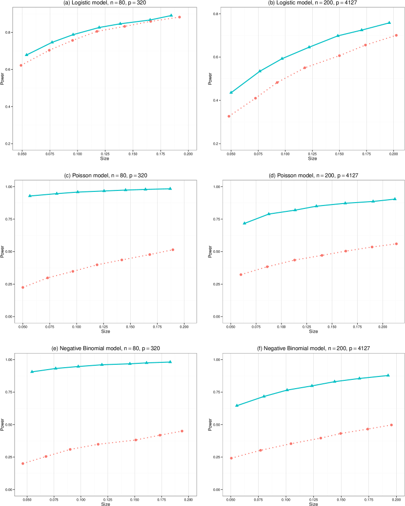
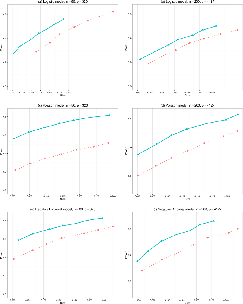
Three generalized linear models were considered in the simulation study: the logistic,
Poisson and Negative Binomial regression models respectively. In the
logistic regression model, the conditional mean of the response Y 𝑌 Y
E ( Y i | X i ) = g ( X i T β ) = exp ( X i T β ) 1 + exp ( X i T β ) , 𝐸 conditional subscript 𝑌 𝑖 subscript 𝑋 𝑖 𝑔 superscript subscript 𝑋 𝑖 T 𝛽 exp superscript subscript 𝑋 𝑖 T 𝛽 1 exp superscript subscript 𝑋 𝑖 T 𝛽 E(Y_{i}|X_{i})=g(X_{i}^{{\mathrm{\scriptscriptstyle T}}}\beta)=\frac{\text{exp}(X_{i}^{{\mathrm{\scriptscriptstyle T}}}\beta)}{1+\text{exp}(X_{i}^{{\mathrm{\scriptscriptstyle T}}}\beta)},
and conditioning on X i subscript 𝑋 𝑖 X_{i} Y i ∼ Bernoulli { 1 , g ( X i T β ) } similar-to subscript 𝑌 𝑖 Bernoulli 1 𝑔 superscript subscript 𝑋 𝑖 T 𝛽 Y_{i}\sim\text{Bernoulli}\{1,g(X_{i}^{{\mathrm{\scriptscriptstyle T}}}\beta)\}
E ( Y i | X i ) = g ( X i T β ) = exp ( X i T β ) , 𝐸 conditional subscript 𝑌 𝑖 subscript 𝑋 𝑖 𝑔 superscript subscript 𝑋 𝑖 T 𝛽 exp superscript subscript 𝑋 𝑖 T 𝛽 E(Y_{i}|X_{i})=g(X_{i}^{{\mathrm{\scriptscriptstyle T}}}\beta)=\text{exp}(X_{i}^{{\mathrm{\scriptscriptstyle T}}}\beta),
and conditioning on X i subscript 𝑋 𝑖 X_{i} Y i ∼ Poisson { g ( X i T β ) } similar-to subscript 𝑌 𝑖 Poisson 𝑔 superscript subscript 𝑋 𝑖 T 𝛽 Y_{i}\sim\text{Poisson}\{g(X_{i}^{{\mathrm{\scriptscriptstyle T}}}\beta)\}
Y | λ ∼ Poisson ( λ ) and λ ∼ Gamma { exp ( X T β ) , 1 } . formulae-sequence similar-to conditional 𝑌 𝜆 Poisson 𝜆 and
similar-to 𝜆 Gamma exp superscript 𝑋 T 𝛽 1 Y|\lambda\sim\text{Poisson}(\lambda)\quad\hbox{and}\quad\lambda\sim\text{Gamma}\{\text{exp}(X^{{\mathrm{\scriptscriptstyle T}}}\beta),1\}.
The conditional distribution of Y 𝑌 Y X 𝑋 X N B { exp ( X T β ) , 1 / 2 } 𝑁 𝐵 exp superscript 𝑋 T 𝛽 1 2 NB\{\text{exp}(X^{{\mathrm{\scriptscriptstyle T}}}\beta),1/2\}
To create regimes of high dimensionality, we chose a relationship
p = exp ( n 0.4 ) 𝑝 exp superscript 𝑛 0.4 p=\text{exp}(n^{0.4}) ( n , p ) = ( 80 , 320 ) 𝑛 𝑝 80 320 (n,p)=(80,320) ( 200 , 4127 ) 200 4127 (200,4127)
We first considered testing the global hypothesis
H 0 : β = 0 p × 1 versus H 1 : β ≠ 0 p × 1 . : subscript 𝐻 0 𝛽 subscript 0 𝑝 1 versus subscript 𝐻 1
: 𝛽 subscript 0 𝑝 1 H_{0}:\beta=0_{p\times 1}\quad\text{versus}\quad H_{1}:\beta\neq 0_{p\times 1}. (6.2)
In designing the alternative hypothesis, we made
‖ β ‖ 2 = 2 superscript norm 𝛽 2 2 \|\beta\|^{2}=2 β 𝛽 \beta Goeman et al. (2011 ) , we restricted
E ( Y i | X i ) 𝐸 conditional subscript 𝑌 𝑖 subscript 𝑋 𝑖 E(Y_{i}|X_{i}) exp ( − 4 ) / { 1 + exp ( − 4 ) } = 0.02 exp 4 1 exp 4 0.02 \text{exp}(-4)/\{1+\text{exp}(-4)\}=0.02 exp ( 4 ) / { 1 + exp ( 4 ) } = 0.98 exp 4 1 exp 4 0.98 \text{exp}(4)/\{1+\text{exp}(4)\}=0.98 exp ( 0 ) = 1 exp 0 1 \text{exp}(0)=1 exp ( 4 ) = 55 exp 4 55 \text{exp}(4)=55
The empirical power profiles (curves of empirical power versus
empirical size) of the global tests for the three generalized linear models were
plotted in Figure 1 Goeman et al. (2011 ) ’s
test had largely similar power profiles for the logistic model as
displayed by Panels (a) and (b) of the figure.
This is consistent with
our findings in
Corollaries 1 2 ℒ β subscript ℒ 𝛽 \mathscr{L}_{\beta} ℒ β subscript ℒ 𝛽 \mathscr{L}_{\beta} 1 Goeman et al. (2011 ) ’s test
in the case of the logistic model. This can be understood as the
impact of A n subscript 𝐴 𝑛 A_{n} S ^ n subscript ^ 𝑆 𝑛 \widehat{S}_{n}
Panels (c)-(f) of Figure 1 g ( ⋅ ) 𝑔 ⋅ g(\cdot) ℒ β F superscript subscript ℒ 𝛽 F \mathscr{L}_{\beta}^{\text{F}} 2 g ( ⋅ ) 𝑔 ⋅ g(\cdot) Goeman et al. (2011 ) ’s test, whereas the
proposed test withstands such situations due to its test statistic
formulation.
We then conducted simulation for testing
H 0 : β ( 2 ) = 0 p 2 × 1 versus H 1 : β ( 2 ) ≠ 0 p 2 × 1 : subscript 𝐻 0 superscript 𝛽 2 subscript 0 subscript 𝑝 2 1 versus subscript 𝐻 1
: superscript 𝛽 2 subscript 0 subscript 𝑝 2 1 H_{0}:\beta^{{\mathrm{\scriptscriptstyle(2)}}}=0_{p_{2}\times 1}\quad\text{versus}\quad H_{1}:\beta^{{\mathrm{\scriptscriptstyle(2)}}}\neq 0_{p_{2}\times 1} (6.3)
in the presence of nuisance
parameter β ( 1 ) superscript 𝛽 1 \beta^{{\mathrm{\scriptscriptstyle(1)}}} β ( 1 ) superscript 𝛽 1 \beta^{{\mathrm{\scriptscriptstyle(1)}}} p 1 = 10 subscript 𝑝 1 10 p_{1}=10 U ( 0 , 1 ) 𝑈 0 1 U(0,1) ( n , p 2 ) = ( 80 , 320 ) 𝑛 subscript 𝑝 2 80 320 (n,p_{2})=(80,320) ( 200 , 4127 ) 200 4127 (200,4127) p 2 = exp ( n 0.4 ) subscript 𝑝 2 exp superscript 𝑛 0.4 p_{2}=\text{exp}(n^{0.4}) β ( 2 ) superscript 𝛽 2 \beta^{{\mathrm{\scriptscriptstyle(2)}}} ‖ β ( 2 ) ‖ 2 = 2 superscript norm superscript 𝛽 2 2 2 \|\beta^{{\mathrm{\scriptscriptstyle(2)}}}\|^{2}=2 β ( 2 ) superscript 𝛽 2 \beta^{{\mathrm{\scriptscriptstyle(2)}}}
The power profiles of the proposed and Goeman et al. (2011 ) ’s tests were displayed in Figure 2 2 n = 80 𝑛 80 n=80 p 2 = 320 subscript 𝑝 2 320 p_{2}=320 Goeman et al. (2011 ) had very
severe size distortion,
which may be due to the
estimation of the nuisance parameter. The test formulation of
Goeman et al. (2011 ) required generating Y ∼ N ( μ ^ 0 , Σ ^ 0 ) similar-to 𝑌 𝑁 subscript ^ 𝜇 0 subscript ^ Σ 0 Y\sim N(\widehat{\mu}_{0},\widehat{\Sigma}_{0}) U ~ n subscript ~ 𝑈 𝑛 \widetilde{U}_{n} n = 200 𝑛 200 n=200 2 n = 80 𝑛 80 n=80 U ~ n subscript ~ 𝑈 𝑛 \widetilde{U}_{n} Y 𝑌 Y μ ^ 0 subscript ^ 𝜇 0 \widehat{\mu}_{0} Σ ^ 0 subscript ^ Σ 0 \widehat{\Sigma}_{0} Goeman et al. (2011 )
was largely absence for the proposed test.
Figure 2 Goeman et al. (2011 ) ’s test. The latter was
similar to the global tests demonstrated in Figure
1
We analyze a dataset that contains microarray readings
for 128 persons who suffer the acute lymphoblastic leukemia.
The dataset also has information on patients’ age, gender and response to multidrug resistance. Among the 128 individuals, 75 of them were patients of the B-cell type leukemia which were classified further to two types: the BCR/ABL fusion ( 35 p a t i e n t s ) 35 𝑝 𝑎 𝑡 𝑖 𝑒 𝑛 𝑡 𝑠 (35~{}patients) ( 40 p a t i e n t s ) 40 𝑝 𝑎 𝑡 𝑖 𝑒 𝑛 𝑡 𝑠 (40~{}patients) Chiaretti et al. (2004 ) , Dudoit et al. (2008 ) ,
Chen and Qin (2010 ) and Li and Chen (2012 ) and others
motivated from different aspects of the inference.
Biological studies have shown that each gene tends to work with
other genes to perform
certain biological missions. Biologists have defined gene-sets under the
Gene Ontology system which provides structured vocabularies
producing names of Gene Ontology terms. The gene-sets under the Gene
Ontology system have been classified to three broad functional
categories:
Biological Processes, Cellular
Components and Molecular Functions. There have been a set of
research works focusing on identifying differentially expressed sets
of genes in the analysis of gene expression data; see
Efron and Tibshirani (2007 ) , Rahmatallah et al. (2012 ) .
After preliminary gene-filtering with the algorithm proposed in
Gentleman et al. (2005 ) , there were 2250 unique Gene Ontology terms
in Biological Processes, 328 in Cellular Component and 402 in
Molecular Function categories respectively, which involved 3265
genes in total.
Our aim here is to identify gene-sets within each functional
category, which are significant in
determining the two types of B-cell acute lymphoblastic leukemia: BCR/ABL fusion or cytogenetically normal NEG.
We formulate it as a binary regression problem with the response
Y i subscript 𝑌 𝑖 Y_{i} i 𝑖 i i 𝑖 i g 𝑔 g X i g = ( X i g ( 1 ) T , X i g ( 2 ) T ) T subscript 𝑋 𝑖 𝑔 superscript subscript superscript 𝑋 1 T 𝑖 𝑔 subscript superscript 𝑋 2 T 𝑖 𝑔 T X_{ig}=(X^{{\mathrm{\scriptscriptstyle(1)}}{\mathrm{\scriptscriptstyle T}}}_{ig},X^{{\mathrm{\scriptscriptstyle(2)}}{\mathrm{\scriptscriptstyle T}}}_{ig})^{{\mathrm{\scriptscriptstyle T}}} X i g ( 1 ) subscript superscript 𝑋 1 𝑖 𝑔 X^{{\mathrm{\scriptscriptstyle(1)}}}_{ig} X i g ( 2 ) subscript superscript 𝑋 2 𝑖 𝑔 X^{{\mathrm{\scriptscriptstyle(2)}}}_{ig} g 𝑔 g
We considered the logistic and probit models
for the gene-set data due to the binary nature of the response
variable.
The two models are, respectively,
E ( Y i | X i g ( 1 ) , X i g ( 2 ) ) = exp ( X i g ( 1 ) T β g ( 1 ) + X i g ( 2 ) T β g ( 2 ) ) 1 + exp ( X i g ( 1 ) T β g ( 1 ) + X i g ( 2 ) T β g ( 2 ) ) and 𝐸 conditional subscript 𝑌 𝑖 subscript superscript 𝑋 1 𝑖 𝑔 subscript superscript 𝑋 2 𝑖 𝑔
exp subscript superscript 𝑋 1 T 𝑖 𝑔 subscript superscript 𝛽 1 𝑔 subscript superscript 𝑋 2 T 𝑖 𝑔 subscript superscript 𝛽 2 𝑔 1 exp subscript superscript 𝑋 1 T 𝑖 𝑔 subscript superscript 𝛽 1 𝑔 subscript superscript 𝑋 2 T 𝑖 𝑔 subscript superscript 𝛽 2 𝑔 and
E(Y_{i}|X^{{\mathrm{\scriptscriptstyle(1)}}}_{ig},X^{{\mathrm{\scriptscriptstyle(2)}}}_{ig})=\frac{\text{exp}(X^{{\mathrm{\scriptscriptstyle(1)}}{\mathrm{\scriptscriptstyle T}}}_{ig}\beta^{{\mathrm{\scriptscriptstyle(1)}}}_{g}+X^{{\mathrm{\scriptscriptstyle(2)}}{\mathrm{\scriptscriptstyle T}}}_{ig}\beta^{{\mathrm{\scriptscriptstyle(2)}}}_{g})}{1+\text{exp}(X^{{\mathrm{\scriptscriptstyle(1)}}{\mathrm{\scriptscriptstyle T}}}_{ig}\beta^{{\mathrm{\scriptscriptstyle(1)}}}_{g}+X^{{\mathrm{\scriptscriptstyle(2)}}{\mathrm{\scriptscriptstyle T}}}_{ig}\beta^{{\mathrm{\scriptscriptstyle(2)}}}_{g})}\quad\text{and}\quad
E ( Y i | X i g ( 1 ) , X i g ( 2 ) ) = Φ ( X i g ( 1 ) T β g ( 1 ) + X i g ( 2 ) T β g ( 2 ) ) . 𝐸 conditional subscript 𝑌 𝑖 subscript superscript 𝑋 1 𝑖 𝑔 subscript superscript 𝑋 2 𝑖 𝑔
Φ subscript superscript 𝑋 1 T 𝑖 𝑔 subscript superscript 𝛽 1 𝑔 subscript superscript 𝑋 2 T 𝑖 𝑔 subscript superscript 𝛽 2 𝑔 E(Y_{i}|X^{{\mathrm{\scriptscriptstyle(1)}}}_{ig},X^{{\mathrm{\scriptscriptstyle(2)}}}_{ig})=\Phi(X^{{\mathrm{\scriptscriptstyle(1)}}{\mathrm{\scriptscriptstyle T}}}_{ig}\beta^{{\mathrm{\scriptscriptstyle(1)}}}_{g}+X^{{\mathrm{\scriptscriptstyle(2)}}{\mathrm{\scriptscriptstyle T}}}_{ig}\beta^{{\mathrm{\scriptscriptstyle(2)}}}_{g}).
For the leukemia data, it is of fundamental interest in discovering
significant Gene Ontology terms while considering the effects of the
three covariates in X ( 1 ) superscript 𝑋 1 X^{{\mathrm{\scriptscriptstyle(1)}}} β g ( 1 ) superscript subscript 𝛽 𝑔 1 \beta_{g}^{{\mathrm{\scriptscriptstyle(1)}}}
H 0 : β g ( 2 ) = 0 versus H 1 : β g ( 2 ) ≠ 0 . : subscript 𝐻 0 subscript superscript 𝛽 2 𝑔 0 versus subscript 𝐻 1
: subscript superscript 𝛽 2 𝑔 0 H_{0}:~{}\beta^{{\mathrm{\scriptscriptstyle(2)}}}_{g}=0\quad\text{versus}\quad H_{1}:~{}\beta^{{\mathrm{\scriptscriptstyle(2)}}}_{g}\neq 0.
By controlling the false discovery rate
(Benjamini and Hochberg, 1995 ) at 0.01, 1084 gene-sets in
Biological Processes, 154 in Cellular Components and 153 in
Molecular Function were found significant under the logistic model,
and 981 in Biological Processes, 140 in Cellular Components and 132
in Molecular Function were significant under the probit model.
Table1
We also carried out the global test for the significance of the
entire regression coefficient vector β g subscript 𝛽 𝑔 \beta_{g}
H 0 : β g = 0 versus H 1 : β g ≠ 0 : subscript 𝐻 0 subscript 𝛽 𝑔 0 versus subscript 𝐻 1
: subscript 𝛽 𝑔 0 H_{0}:~{}\beta_{g}=0\quad\text{versus}\quad H_{1}:~{}\beta_{g}\neq 0
where
β g = ( β g ( 1 ) T , β g ( 2 ) T ) T subscript 𝛽 𝑔 superscript superscript subscript 𝛽 𝑔 1 T superscript subscript 𝛽 𝑔 2 T T \beta_{g}=(\beta_{g}^{{\mathrm{\scriptscriptstyle(1)}}{\mathrm{\scriptscriptstyle T}}},\beta_{g}^{{\mathrm{\scriptscriptstyle(2)}}{\mathrm{\scriptscriptstyle T}}})^{{\mathrm{\scriptscriptstyle T}}} H 0 subscript 𝐻 0 H_{0} g ( X i T β g ) = g ( 0 ) = 0.5 𝑔 superscript subscript 𝑋 𝑖 T subscript 𝛽 𝑔 𝑔 0 0.5 g(X_{i}^{{\mathrm{\scriptscriptstyle T}}}\beta_{g})=g(0)=0.5 ψ ( X i , 0 ) 𝜓 subscript 𝑋 𝑖 0 \psi(X_{i},0) ψ ( X i , 0 ) 𝜓 subscript 𝑋 𝑖 0 \psi(X_{i},0)
Figure 3 L n subscript 𝐿 𝑛 L_{n} 3 4 5 3 4 5 4 5 3
As the generalized linear models are widely used tools in analyzing genetic data, the proposed tests, being more
adaptive to the high dimensionality, are useful additions to the existing
test procedures for the significance of regression coefficients. As
shown in the case study, testing for the significance of gene-sets
requires high dimensional multivariate test procedures which can produce
p-values under both high dimensionality and multiplicity (as genes in
gene-sets can overlap). The proposed tests and the tests of
Goeman et al. (2011 ) are such tests which can
be used for the gene-sets testing in conjunction with the FDR
procedure to control the overall family-wise error rate when testing
a large number of hypotheses simultaneously.
The test of Goeman et al. (2011 ) was proposed
for fixed dimension p 𝑝 p n 𝑛 n Goeman et al. (2011 ) ’s test
in the context of high dimensionality. This is especially the case when the
inverse of the link function is unbounded, which permits the high dimensionality to insert adverse influence on the test of
Goeman et al. (2011 ) . The proposed test
statistics due to their simpler formulations can avoid some of the
high dimensional effects, and hence lead to better test performances in terms
of more accurate size approximation and more power in detecting the
significant regression coefficient vector.
In this section, we provide technical proofs to the main results
reported in Section 3-5. To establish the results of the paper, we
introduce three lemmas whose proofs are available in
Chen and Guo (2014 ) .
We define a few notations:
ϵ i = Y i − g ( X i T β ) , ϵ 0 i = Y i − g ( X i T β 0 ) , V 0 i = V { g ( X i T β 0 ) } , ψ 0 i = g ′ ( X i T β 0 ) / V { g ( X i T β 0 ) } . formulae-sequence subscript italic-ϵ 𝑖 subscript 𝑌 𝑖 𝑔 superscript subscript 𝑋 𝑖 T 𝛽 formulae-sequence subscript italic-ϵ 0 𝑖 subscript 𝑌 𝑖 𝑔 superscript subscript 𝑋 𝑖 T subscript 𝛽 0 formulae-sequence subscript 𝑉 0 𝑖 𝑉 𝑔 superscript subscript 𝑋 𝑖 T subscript 𝛽 0 subscript 𝜓 0 𝑖 superscript 𝑔 ′ superscript subscript 𝑋 𝑖 T subscript 𝛽 0 𝑉 𝑔 superscript subscript 𝑋 𝑖 T subscript 𝛽 0 \epsilon_{i}=Y_{i}-g(X_{i}^{{\mathrm{\scriptscriptstyle T}}}\beta),\quad\epsilon_{0i}=Y_{i}-g(X_{i}^{{\mathrm{\scriptscriptstyle T}}}\beta_{0}),\quad V_{0i}=V\{g(X_{i}^{{\mathrm{\scriptscriptstyle T}}}\beta_{0})\},\quad\psi_{0i}=g^{\prime}(X_{i}^{{\mathrm{\scriptscriptstyle T}}}\beta_{0})/V\{g(X_{i}^{{\mathrm{\scriptscriptstyle T}}}\beta_{0})\}.
Lemma A.1 .
The expectations and variances of A n subscript 𝐴 𝑛 A_{n} U n subscript 𝑈 𝑛 U_{n}
μ A n = tr { Σ β ( β 0 ) + Ξ β , β 0 } , μ U n = ( n − 1 ) Δ β , β 0 T Δ β , β 0 , formulae-sequence subscript 𝜇 subscript A 𝑛 tr subscript Σ 𝛽 subscript 𝛽 0 subscript Ξ 𝛽 subscript 𝛽 0
subscript 𝜇 subscript U 𝑛 𝑛 1 superscript subscript Δ 𝛽 subscript 𝛽 0
T subscript Δ 𝛽 subscript 𝛽 0
\mu_{{\mathrm{\scriptscriptstyle A}_{n}}}=\mathrm{tr}\{\Sigma_{\beta}(\beta_{0})+\Xi_{\beta,\beta_{0}}\},\quad\mu_{{\mathrm{\scriptscriptstyle U}_{n}}}=(n-1)\Delta_{\beta,\beta_{0}}^{{\mathrm{\scriptscriptstyle T}}}\Delta_{\beta,\beta_{0}},
σ A n 2 = n − 1 [ E { ϵ 0 4 ψ 0 4 ( X T X ) 2 } − E 2 { ϵ 0 2 ψ 0 2 ( X T X ) } ] and superscript subscript 𝜎 subscript A 𝑛 2 superscript 𝑛 1 delimited-[] 𝐸 superscript subscript italic-ϵ 0 4 subscript superscript 𝜓 4 0 superscript superscript 𝑋 T 𝑋 2 superscript 𝐸 2 superscript subscript italic-ϵ 0 2 subscript superscript 𝜓 2 0 superscript 𝑋 T 𝑋 and
\sigma_{{\mathrm{\scriptscriptstyle A}_{n}}}^{2}={n^{-1}}\bigl{[}E\bigl{\{}\epsilon_{0}^{4}\psi^{4}_{0}(X^{\mathrm{\scriptscriptstyle T}}X)^{2}\bigr{\}}-E^{2}\bigl{\{}\epsilon_{0}^{2}\psi^{2}_{0}(X^{\mathrm{\scriptscriptstyle T}}X)\bigr{\}}\bigr{]}\quad\hbox{and}\quad
σ U n 2 = 4 ( n − 2 ) ( 1 − n − 1 ) ξ 1 + 2 ( 1 − n − 1 ) ξ 2 superscript subscript 𝜎 subscript U 𝑛 2 4 𝑛 2 1 superscript 𝑛 1 subscript 𝜉 1 2 1 superscript 𝑛 1 subscript 𝜉 2 \sigma_{{\mathrm{\scriptscriptstyle U}_{n}}}^{2}={4(n-2)(1-n^{-1})}\xi_{1}+{2(1-n^{-1})}\xi_{2}
where ξ 1 = Δ β , β 0 T { Σ β ( β 0 ) + Ξ β , β 0 } Δ β , β 0 − ( Δ β , β 0 T Δ β , β 0 ) 2 subscript 𝜉 1 superscript subscript Δ 𝛽 subscript 𝛽 0
T subscript Σ 𝛽 subscript 𝛽 0 subscript Ξ 𝛽 subscript 𝛽 0
subscript Δ 𝛽 subscript 𝛽 0
superscript superscript subscript Δ 𝛽 subscript 𝛽 0
T subscript Δ 𝛽 subscript 𝛽 0
2 \xi_{1}=\Delta_{\beta,\beta_{0}}^{{\mathrm{\scriptscriptstyle T}}}\{\Sigma_{\beta}(\beta_{0})+\Xi_{\beta,\beta_{0}}\}\Delta_{\beta,\beta_{0}}-(\Delta_{\beta,\beta_{0}}^{{\mathrm{\scriptscriptstyle T}}}\Delta_{\beta,\beta_{0}})^{2} ξ 2 = tr { Σ β ( β 0 ) + Ξ β , β 0 } 2 − ( Δ β , β 0 T Δ β , β 0 ) 2 . subscript 𝜉 2 tr superscript subscript Σ 𝛽 subscript 𝛽 0 subscript Ξ 𝛽 subscript 𝛽 0
2 superscript superscript subscript Δ 𝛽 subscript 𝛽 0
T subscript Δ 𝛽 subscript 𝛽 0
2 \xi_{2}=\mathrm{tr}\{\Sigma_{\beta}(\beta_{0})+\Xi_{\beta,\beta_{0}}\}^{2}-(\Delta_{\beta,\beta_{0}}^{{\mathrm{\scriptscriptstyle T}}}\Delta_{\beta,\beta_{0}})^{2}.
Lemma A.2 .
Under Assumptions 3.1 3.4 ℒ β subscript ℒ 𝛽 \mathscr{L}_{\beta}
σ U n 2 = 2 t r { Σ β ( β 0 ) + Ξ β , β 0 } 2 { 1 + o ( 1 ) } as n → ∞ . subscript superscript 𝜎 2 subscript U 𝑛 2 t r superscript subscript Σ 𝛽 subscript 𝛽 0 subscript Ξ 𝛽 subscript 𝛽 0
2 1 𝑜 1 as n → ∞ .
\sigma^{2}_{{\mathrm{\scriptscriptstyle U}_{n}}}=2\mathrm{tr}\{\Sigma_{\beta}(\beta_{0})+\Xi_{\beta,\beta_{0}}\}^{2}\{1+o(1)\}\quad\mbox{as $n\to\infty$.}
Lemma A.3 .
Under Assumptions 3.1 3.4 ℒ β subscript ℒ 𝛽 \mathscr{L}_{\beta}
tr { Σ β 0 2 ( β 0 ) } ^ tr { Σ β ( β 0 ) + Ξ β , β 0 } 2 → 1 and tr { Σ β 0 ( β 0 ) } ^ tr { Σ β ( β 0 ) + Ξ β , β 0 } → 1 formulae-sequence → ^ tr subscript superscript Σ 2 subscript 𝛽 0 subscript 𝛽 0 tr superscript subscript Σ 𝛽 subscript 𝛽 0 subscript Ξ 𝛽 subscript 𝛽 0
2 1 and
→ ^ tr subscript Σ subscript 𝛽 0 subscript 𝛽 0 tr subscript Σ 𝛽 subscript 𝛽 0 subscript Ξ 𝛽 subscript 𝛽 0
1 \frac{\widehat{\mathrm{tr}\{\Sigma^{2}_{\beta_{0}}(\beta_{0})\}}}{\mathrm{tr}\{\Sigma_{\beta}(\beta_{0})+\Xi_{\beta,\beta_{0}}\}^{2}}\to 1\quad\text{and}\quad\frac{\widehat{\mathrm{tr}\{\Sigma_{\beta_{0}}(\beta_{0})\}}}{\mathrm{tr}\{\Sigma_{\beta}(\beta_{0})+\Xi_{\beta,\beta_{0}}\}}\to 1
in probability as n → ∞ → 𝑛 n\to\infty
In the following, we provide technical proofs for the
main results in Section 4 first, since they are used to establish
the results in Section 3. The results in Section 5 are given the
last.
Define
σ n 2 = 2 t r { Σ β ( β 0 ) + Ξ β , β 0 } 2 subscript superscript 𝜎 2 𝑛 2 t r superscript subscript Σ 𝛽 subscript 𝛽 0 subscript Ξ 𝛽 subscript 𝛽 0
2 \sigma^{2}_{n}=2\mathrm{tr}\{\Sigma_{\beta}(\beta_{0})+\Xi_{\beta,\beta_{0}}\}^{2}
U n − ( n − 1 ) Δ β , β 0 T Δ β , β 0 = V n 1 + V n 2 where subscript 𝑈 𝑛 𝑛 1 superscript subscript Δ 𝛽 subscript 𝛽 0
T subscript Δ 𝛽 subscript 𝛽 0
subscript 𝑉 𝑛 1 subscript 𝑉 𝑛 2 where
U_{n}-(n-1)\Delta_{\beta,\beta_{0}}^{{\mathrm{\scriptscriptstyle T}}}\Delta_{\beta,\beta_{0}}=V_{n1}+V_{n2}\quad\text{where}
V n 1 = 1 n ∑ i ≠ j n ( Δ β , β 0 T ϵ 0 j ψ 0 j X j + Δ β , β 0 T ϵ 0 i ψ 0 i X i − 2 Δ β , β 0 T Δ β , β 0 ) and subscript 𝑉 𝑛 1 1 𝑛 superscript subscript 𝑖 𝑗 𝑛 superscript subscript Δ 𝛽 subscript 𝛽 0
T subscript italic-ϵ 0 𝑗 subscript 𝜓 0 𝑗 subscript 𝑋 𝑗 superscript subscript Δ 𝛽 subscript 𝛽 0
T subscript italic-ϵ 0 𝑖 subscript 𝜓 0 𝑖 subscript 𝑋 𝑖 2 superscript subscript Δ 𝛽 subscript 𝛽 0
T subscript Δ 𝛽 subscript 𝛽 0
and
V_{n1}=\frac{1}{n}\sum\limits_{i\neq j}^{n}(\Delta_{\beta,\beta_{0}}^{{\mathrm{\scriptscriptstyle T}}}\epsilon_{0j}\psi_{0j}X_{j}+\Delta_{\beta,\beta_{0}}^{{\mathrm{\scriptscriptstyle T}}}\epsilon_{0i}\psi_{0i}X_{i}-2\Delta_{\beta,\beta_{0}}^{{\mathrm{\scriptscriptstyle T}}}\Delta_{\beta,\beta_{0}})\quad\text{and}\quad
V n 2 = 1 n ∑ i ≠ j n ( ϵ 0 i ψ 0 i X i − Δ β , β 0 ) T ( ϵ 0 j ψ 0 j X j − Δ β , β 0 ) . subscript 𝑉 𝑛 2 1 𝑛 superscript subscript 𝑖 𝑗 𝑛 superscript subscript italic-ϵ 0 𝑖 subscript 𝜓 0 𝑖 subscript 𝑋 𝑖 subscript Δ 𝛽 subscript 𝛽 0
T subscript italic-ϵ 0 𝑗 subscript 𝜓 0 𝑗 subscript 𝑋 𝑗 subscript Δ 𝛽 subscript 𝛽 0
V_{n2}=\frac{1}{n}\sum\limits_{i\neq j}^{n}(\epsilon_{0i}\psi_{0i}X_{i}-\Delta_{\beta,\beta_{0}})^{{\mathrm{\scriptscriptstyle T}}}(\epsilon_{0j}\psi_{0j}X_{j}-\Delta_{\beta,\beta_{0}}).
As E ( V n 1 ) = 0 𝐸 subscript 𝑉 𝑛 1 0 E(V_{n1})=0 A.1 ℒ β subscript ℒ 𝛽 \mathscr{L}_{\beta}
var ( V n 1 ) = o ( σ n 2 ) and V n 1 = o p ( σ n ) . formulae-sequence var subscript 𝑉 𝑛 1 𝑜 subscript superscript 𝜎 2 𝑛 and
subscript 𝑉 𝑛 1 subscript 𝑜 𝑝 subscript 𝜎 𝑛 \text{var}(V_{n1})=o(\sigma^{2}_{n})\quad\text{and}\quad V_{n1}=o_{p}(\sigma_{n}).
We use the martingale central limit
theorem to show the asymptotic normality of V n 2 subscript 𝑉 𝑛 2 V_{n2}
Z n , i = 2 n σ n ∑ j = 1 i − 1 ( ϵ 0 i ψ 0 i X i − Δ β , β 0 ) T ( ϵ 0 j ψ 0 j X j − Δ β , β 0 ) for i ≥ 2 , and formulae-sequence subscript 𝑍 𝑛 𝑖
2 𝑛 subscript 𝜎 𝑛 superscript subscript 𝑗 1 𝑖 1 superscript subscript italic-ϵ 0 𝑖 subscript 𝜓 0 𝑖 subscript 𝑋 𝑖 subscript Δ 𝛽 subscript 𝛽 0
T subscript italic-ϵ 0 𝑗 subscript 𝜓 0 𝑗 subscript 𝑋 𝑗 subscript Δ 𝛽 subscript 𝛽 0
for 𝑖 2 and
Z_{n,i}=\frac{2}{n\sigma_{n}}\sum_{j=1}^{i-1}(\epsilon_{0i}\psi_{0i}X_{i}-\Delta_{\beta,\beta_{0}})^{{\mathrm{\scriptscriptstyle T}}}(\epsilon_{0j}\psi_{0j}X_{j}-\Delta_{\beta,\beta_{0}})\quad\mbox{for}~{}i\geq 2,~{}\mbox{and}
T n , k = ∑ i = 2 k Z n , i . subscript 𝑇 𝑛 𝑘
superscript subscript 𝑖 2 𝑘 subscript 𝑍 𝑛 𝑖
T_{n,k}=\sum_{i=2}^{k}Z_{n,i}. T n , n = ∑ i = 2 n Z n , i = V n 2 / σ n . subscript 𝑇 𝑛 𝑛
superscript subscript 𝑖 2 𝑛 subscript 𝑍 𝑛 𝑖
subscript 𝑉 𝑛 2 subscript 𝜎 𝑛 T_{n,n}=\sum_{i=2}^{n}Z_{n,i}={V_{n2}}/{\sigma_{n}}.
Let ℱ k = σ { ( X 1 ϵ 1 ) , … , ( X k ϵ k ) } subscript ℱ 𝑘 𝜎 subscript 𝑋 1 subscript italic-ϵ 1 … subscript 𝑋 𝑘 subscript italic-ϵ 𝑘 \mathscr{F}_{k}=\sigma\left\{\left(\begin{smallmatrix}X_{1}\\
\epsilon_{1}\end{smallmatrix}\right),\ldots,\left(\begin{smallmatrix}X_{k}\\
\epsilon_{k}\end{smallmatrix}\right)\right\} σ 𝜎 \sigma ( X i ϵ i ) subscript 𝑋 𝑖 subscript italic-ϵ 𝑖 \bigl{(}\begin{smallmatrix}X_{i}\\
\epsilon_{i}\end{smallmatrix}\bigr{)} i = 1 , … , k . 𝑖 1 … 𝑘
i=1,\ldots,k. T n , k subscript 𝑇 𝑛 𝑘
T_{n,k} i = 2 , … , n 𝑖 2 … 𝑛
i=2,\ldots,n v n , i = E ( Z n , i 2 | ℱ i − 1 ) subscript 𝑣 𝑛 𝑖
𝐸 conditional superscript subscript 𝑍 𝑛 𝑖
2 subscript ℱ 𝑖 1 v_{n,i}=E(Z_{n,i}^{2}|\mathscr{F}_{i-1}) v n = ∑ i = 2 n v n , i subscript 𝑣 𝑛 superscript subscript 𝑖 2 𝑛 subscript 𝑣 𝑛 𝑖
v_{n}=\sum_{i=2}^{n}v_{n,i}
From Hall and Heyde (1980 ) , in order to show the asymptotic
normality of V n 2 subscript 𝑉 𝑛 2 V_{n2}
v n → 1 in probability as n → ∞ ; → subscript 𝑣 𝑛 1 in probability as n → ∞
v_{n}\to 1\quad\mbox{in probability as $n\to\infty$}; (A.1)
for any η > 0 , ∑ i = 2 n E { Z n , i 2 I ( | Z n , i | > η ) } → 0 as n → ∞ . formulae-sequence for any 𝜂 0 → superscript subscript 𝑖 2 𝑛 𝐸 superscript subscript 𝑍 𝑛 𝑖
2 𝐼 subscript 𝑍 𝑛 𝑖
𝜂 0 as n → ∞ . \text{for any}~{}\eta>0,~{}\sum_{i=2}^{n}E\{Z_{n,i}^{2}I(|Z_{n,i}|>\eta)\}\rightarrow 0~{}~{}\text{as $n\to\infty.$} (A.2)
We first establish (A.1 i = 2 , … , n , 𝑖 2 … 𝑛
i=2,\dots,n,
v n , i = 4 n 2 σ n 2 [ ∑ j = 1 i − 1 ( ϵ 0 j ψ 0 j X j − Δ β , β 0 ) T { Σ β ( β 0 ) + Ξ β , β 0 − Δ β , β 0 Δ β , β 0 T } ( ϵ 0 j ψ 0 j X j − Δ β , β 0 ) + ∑ j 1 ≠ j 2 i − 1 ( ϵ 0 j 1 ψ 0 j 1 X j 1 − Δ β , β 0 ) T { Σ β ( β 0 ) + Ξ β , β 0 − Δ β , β 0 Δ β , β 0 T } ( ϵ 0 j 2 ψ 0 j 2 X j 2 − Δ β , β 0 ) ] . subscript 𝑣 𝑛 𝑖
4 superscript 𝑛 2 superscript subscript 𝜎 𝑛 2 delimited-[] superscript subscript 𝑗 1 𝑖 1 superscript subscript italic-ϵ 0 𝑗 subscript 𝜓 0 𝑗 subscript 𝑋 𝑗 subscript Δ 𝛽 subscript 𝛽 0
T subscript Σ 𝛽 subscript 𝛽 0 subscript Ξ 𝛽 subscript 𝛽 0
subscript Δ 𝛽 subscript 𝛽 0
superscript subscript Δ 𝛽 subscript 𝛽 0
T subscript italic-ϵ 0 𝑗 subscript 𝜓 0 𝑗 subscript 𝑋 𝑗 subscript Δ 𝛽 subscript 𝛽 0
superscript subscript subscript 𝑗 1 subscript 𝑗 2 𝑖 1 superscript subscript italic-ϵ 0 subscript 𝑗 1 subscript 𝜓 0 subscript 𝑗 1 subscript 𝑋 subscript 𝑗 1 subscript Δ 𝛽 subscript 𝛽 0
T subscript Σ 𝛽 subscript 𝛽 0 subscript Ξ 𝛽 subscript 𝛽 0
subscript Δ 𝛽 subscript 𝛽 0
superscript subscript Δ 𝛽 subscript 𝛽 0
T subscript italic-ϵ 0 subscript 𝑗 2 subscript 𝜓 0 subscript 𝑗 2 subscript 𝑋 subscript 𝑗 2 subscript Δ 𝛽 subscript 𝛽 0
\begin{split}v_{n,i}=&\frac{4}{n^{2}\sigma_{n}^{2}}\bigg{[}\sum_{j=1}^{i-1}(\epsilon_{0j}\psi_{0j}X_{j}-\Delta_{\beta,\beta_{0}})^{{\mathrm{\scriptscriptstyle T}}}\{\Sigma_{\beta}(\beta_{0})+\Xi_{\beta,\beta_{0}}-\Delta_{\beta,\beta_{0}}\Delta_{\beta,\beta_{0}}^{{\mathrm{\scriptscriptstyle T}}}\}(\epsilon_{0j}\psi_{0j}X_{j}-\Delta_{\beta,\beta_{0}})\\
&+\sum_{j_{1}\neq j_{2}}^{i-1}(\epsilon_{0j_{1}}\psi_{0j_{1}}X_{j_{1}}-\Delta_{\beta,\beta_{0}})^{{\mathrm{\scriptscriptstyle T}}}\{\Sigma_{\beta}(\beta_{0})+\Xi_{\beta,\beta_{0}}-\Delta_{\beta,\beta_{0}}\Delta_{\beta,\beta_{0}}^{{\mathrm{\scriptscriptstyle T}}}\}(\epsilon_{0j_{2}}\psi_{0j_{2}}X_{j_{2}}-\Delta_{\beta,\beta_{0}})\bigg{]}.\end{split}
Then
v n = ∑ i = 2 n v n , i = C 1 + C 2 where formulae-sequence subscript 𝑣 𝑛 superscript subscript 𝑖 2 𝑛 subscript 𝑣 𝑛 𝑖
subscript 𝐶 1 subscript 𝐶 2 where v_{n}=\sum_{i=2}^{n}v_{n,i}=C_{1}+C_{2}\quad\text{where}
C 1 = 4 n 2 σ n 2 ∑ j = 1 n − 1 [ ( n − j ) ( ϵ 0 j ψ 0 j X j − Δ β , β 0 ) T { Σ β ( β 0 ) + Ξ β , β 0 − Δ β , β 0 Δ β , β 0 T } ( ϵ 0 j ψ 0 j X j − Δ β , β 0 ) ] and subscript 𝐶 1 4 superscript 𝑛 2 superscript subscript 𝜎 𝑛 2 superscript subscript 𝑗 1 𝑛 1 delimited-[] 𝑛 𝑗 superscript subscript italic-ϵ 0 𝑗 subscript 𝜓 0 𝑗 subscript 𝑋 𝑗 subscript Δ 𝛽 subscript 𝛽 0
T subscript Σ 𝛽 subscript 𝛽 0 subscript Ξ 𝛽 subscript 𝛽 0
subscript Δ 𝛽 subscript 𝛽 0
superscript subscript Δ 𝛽 subscript 𝛽 0
T subscript italic-ϵ 0 𝑗 subscript 𝜓 0 𝑗 subscript 𝑋 𝑗 subscript Δ 𝛽 subscript 𝛽 0
and C_{1}=\frac{4}{n^{2}\sigma_{n}^{2}}\sum_{j=1}^{n-1}\bigl{[}(n-j)(\epsilon_{0j}\psi_{0j}X_{j}-\Delta_{\beta,\beta_{0}})^{{\mathrm{\scriptscriptstyle T}}}\{\Sigma_{\beta}(\beta_{0})+\Xi_{\beta,\beta_{0}}-\Delta_{\beta,\beta_{0}}\Delta_{\beta,\beta_{0}}^{{\mathrm{\scriptscriptstyle T}}}\}(\epsilon_{0j}\psi_{0j}X_{j}-\Delta_{\beta,\beta_{0}})\bigr{]}~{}~{}\text{and}
C 2 = 8 n 2 σ n 2 ∑ 1 ≤ j 1 < j 2 ≤ n − 1 [ ( n − j 2 ) ( ϵ 0 j 1 ψ 0 j 1 X j 1 − Δ β , β 0 ) T { Σ β ( β 0 ) + Ξ β , β 0 − Δ β , β 0 Δ β , β 0 T } ( ϵ 0 j 2 ψ 0 j 2 X j 2 − Δ β , β 0 ) ] . subscript 𝐶 2 8 superscript 𝑛 2 superscript subscript 𝜎 𝑛 2 subscript 1 subscript 𝑗 1 subscript 𝑗 2 𝑛 1 delimited-[] 𝑛 subscript 𝑗 2 superscript subscript italic-ϵ 0 subscript 𝑗 1 subscript 𝜓 0 subscript 𝑗 1 subscript 𝑋 subscript 𝑗 1 subscript Δ 𝛽 subscript 𝛽 0
T subscript Σ 𝛽 subscript 𝛽 0 subscript Ξ 𝛽 subscript 𝛽 0
subscript Δ 𝛽 subscript 𝛽 0
superscript subscript Δ 𝛽 subscript 𝛽 0
T subscript italic-ϵ 0 subscript 𝑗 2 subscript 𝜓 0 subscript 𝑗 2 subscript 𝑋 subscript 𝑗 2 subscript Δ 𝛽 subscript 𝛽 0
C_{2}=\frac{8}{n^{2}\sigma_{n}^{2}}\sum_{1\leq j_{1}<j_{2}\leq n-1}\bigl{[}(n-j_{2})(\epsilon_{0j_{1}}\psi_{0j_{1}}X_{j_{1}}-\Delta_{\beta,\beta_{0}})^{{\mathrm{\scriptscriptstyle T}}}\{\Sigma_{\beta}(\beta_{0})+\Xi_{\beta,\beta_{0}}-\Delta_{\beta,\beta_{0}}\Delta_{\beta,\beta_{0}}^{{\mathrm{\scriptscriptstyle T}}}\}(\epsilon_{0j_{2}}\psi_{0j_{2}}X_{j_{2}}-\Delta_{\beta,\beta_{0}})\bigr{]}.
Under the “local” alternatives ℒ β subscript ℒ 𝛽 \mathscr{L}_{\beta}
E [ ( ϵ 0 j ψ 0 j X j − Δ β , β 0 ) T { Σ β ( β 0 ) + Ξ β , β 0 − Δ β , β 0 Δ β , β 0 T } ( ϵ 0 j ψ 0 j X j − Δ β , β 0 ) ] = tr { Σ β ( β 0 ) + Ξ β , β 0 } 2 { 1 + o ( 1 ) } . 𝐸 delimited-[] superscript subscript italic-ϵ 0 𝑗 subscript 𝜓 0 𝑗 subscript 𝑋 𝑗 subscript Δ 𝛽 subscript 𝛽 0
T subscript Σ 𝛽 subscript 𝛽 0 subscript Ξ 𝛽 subscript 𝛽 0
subscript Δ 𝛽 subscript 𝛽 0
superscript subscript Δ 𝛽 subscript 𝛽 0
T subscript italic-ϵ 0 𝑗 subscript 𝜓 0 𝑗 subscript 𝑋 𝑗 subscript Δ 𝛽 subscript 𝛽 0
tr superscript subscript Σ 𝛽 subscript 𝛽 0 subscript Ξ 𝛽 subscript 𝛽 0
2 1 𝑜 1 E\bigl{[}(\epsilon_{0j}\psi_{0j}X_{j}-\Delta_{\beta,\beta_{0}})^{{\mathrm{\scriptscriptstyle T}}}\{\Sigma_{\beta}(\beta_{0})+\Xi_{\beta,\beta_{0}}-\Delta_{\beta,\beta_{0}}\Delta_{\beta,\beta_{0}}^{{\mathrm{\scriptscriptstyle T}}}\}(\epsilon_{0j}\psi_{0j}X_{j}-\Delta_{\beta,\beta_{0}})\bigr{]}=\text{tr}\{\Sigma_{\beta}(\beta_{0})+\Xi_{\beta,\beta_{0}}\}^{2}\{1+o(1)\}.
Thus E ( C 1 ) = 1 + o ( 1 ) . 𝐸 subscript 𝐶 1 1 𝑜 1 E(C_{1})={1+o(1)}. Chen and Guo (2014 ) ,
var ( C 1 ) = 16 n 4 σ n 4 ∑ j = 1 n − 1 E [ ( n − j ) ( ϵ 0 j ψ 0 j X j − Δ β , β 0 ) T { Σ β ( β 0 ) + Ξ β , β 0 − Δ β , β 0 Δ β , β 0 T } ( ϵ 0 j ψ 0 j X j − Δ β , β 0 ) ] 2 ≤ 16 n 4 σ n 4 ∑ j = 1 n − 1 ( n − j ) 2 O [ tr 2 { Σ β ( β 0 ) + Ξ β , β 0 } 2 ] = O ( n − 1 ) . var subscript 𝐶 1 16 superscript 𝑛 4 superscript subscript 𝜎 𝑛 4 superscript subscript 𝑗 1 𝑛 1 𝐸 superscript delimited-[] 𝑛 𝑗 superscript subscript italic-ϵ 0 𝑗 subscript 𝜓 0 𝑗 subscript 𝑋 𝑗 subscript Δ 𝛽 subscript 𝛽 0
T subscript Σ 𝛽 subscript 𝛽 0 subscript Ξ 𝛽 subscript 𝛽 0
subscript Δ 𝛽 subscript 𝛽 0
superscript subscript Δ 𝛽 subscript 𝛽 0
T subscript italic-ϵ 0 𝑗 subscript 𝜓 0 𝑗 subscript 𝑋 𝑗 subscript Δ 𝛽 subscript 𝛽 0
2 16 superscript 𝑛 4 superscript subscript 𝜎 𝑛 4 superscript subscript 𝑗 1 𝑛 1 superscript 𝑛 𝑗 2 𝑂 delimited-[] superscript tr 2 superscript subscript Σ 𝛽 subscript 𝛽 0 subscript Ξ 𝛽 subscript 𝛽 0
2 𝑂 superscript 𝑛 1 \begin{split}\text{var}(C_{1})&=\frac{16}{n^{4}\sigma_{n}^{4}}\sum_{j=1}^{n-1}E\bigl{[}(n-j)(\epsilon_{0j}\psi_{0j}X_{j}-\Delta_{\beta,\beta_{0}})^{{\mathrm{\scriptscriptstyle T}}}\{\Sigma_{\beta}(\beta_{0})+\Xi_{\beta,\beta_{0}}-\Delta_{\beta,\beta_{0}}\Delta_{\beta,\beta_{0}}^{{\mathrm{\scriptscriptstyle T}}}\}(\epsilon_{0j}\psi_{0j}X_{j}-\Delta_{\beta,\beta_{0}})\bigr{]}^{2}\\
&\leq\frac{16}{n^{4}\sigma_{n}^{4}}\sum_{j=1}^{n-1}(n-j)^{2}O[\text{tr}^{2}\{\Sigma_{\beta}(\beta_{0})+\Xi_{\beta,\beta_{0}}\}^{2}]=O(n^{-1}).\end{split}
Therefore C 1 → 1 → subscript 𝐶 1 1 C_{1}\to 1 C 2 subscript 𝐶 2 C_{2} E ( C 2 ) = 0 𝐸 subscript 𝐶 2 0 E(C_{2})=0
var ( C 2 ) = 64 n 4 σ n 4 ∑ 1 ≤ j 1 < j 2 ≤ n − 1 ( n − j 2 ) 2 tr { Σ β ( β 0 ) + Ξ β , β 0 − Δ β , β 0 Δ β , β 0 T } 4 = o ( 1 ) . var subscript 𝐶 2 64 superscript 𝑛 4 superscript subscript 𝜎 𝑛 4 subscript 1 subscript 𝑗 1 subscript 𝑗 2 𝑛 1 superscript 𝑛 subscript 𝑗 2 2 tr superscript subscript Σ 𝛽 subscript 𝛽 0 subscript Ξ 𝛽 subscript 𝛽 0
subscript Δ 𝛽 subscript 𝛽 0
superscript subscript Δ 𝛽 subscript 𝛽 0
T 4 𝑜 1 \begin{split}\text{var}(C_{2})&=\frac{64}{n^{4}\sigma_{n}^{4}}\sum_{1\leq j_{1}<j_{2}\leq n-1}(n-j_{2})^{2}\text{tr}\{\Sigma_{\beta}(\beta_{0})+\Xi_{\beta,\beta_{0}}-\Delta_{\beta,\beta_{0}}\Delta_{\beta,\beta_{0}}^{{\mathrm{\scriptscriptstyle T}}}\}^{4}=o(1).\\
\end{split}
Thus, C 2 → 0 → subscript 𝐶 2 0 C_{2}\to 0 A.1
Next, we verify (A.2 η > 0 𝜂 0 \eta>0
∑ i = 2 n E { Z n , i 2 I ( | Z n , i | > η ) } ≤ 1 η 2 ∑ i = 2 n E ( Z n , i 4 ) and superscript subscript 𝑖 2 𝑛 𝐸 superscript subscript 𝑍 𝑛 𝑖
2 𝐼 subscript 𝑍 𝑛 𝑖
𝜂 1 superscript 𝜂 2 superscript subscript 𝑖 2 𝑛 𝐸 superscript subscript 𝑍 𝑛 𝑖
4 and
\sum_{i=2}^{n}E\{Z_{n,i}^{2}I(|Z_{n,i}|>\eta)\}\leq\frac{1}{\eta^{2}}\sum_{i=2}^{n}E(Z_{n,i}^{4})\quad\text{and}
∑ i = 2 n E ( Z n , i 4 ) = 16 n 4 σ n 4 ∑ i = 2 n E { ∑ j = 1 i − 1 ( ϵ 0 i ψ 0 i X i − Δ β , β 0 ) T ( ϵ 0 j ψ 0 j X j − Δ β , β 0 ) } 4 = P 1 + P 2 superscript subscript 𝑖 2 𝑛 𝐸 superscript subscript 𝑍 𝑛 𝑖
4 16 superscript 𝑛 4 superscript subscript 𝜎 𝑛 4 superscript subscript 𝑖 2 𝑛 𝐸 superscript superscript subscript 𝑗 1 𝑖 1 superscript subscript italic-ϵ 0 𝑖 subscript 𝜓 0 𝑖 subscript 𝑋 𝑖 subscript Δ 𝛽 subscript 𝛽 0
T subscript italic-ϵ 0 𝑗 subscript 𝜓 0 𝑗 subscript 𝑋 𝑗 subscript Δ 𝛽 subscript 𝛽 0
4 subscript 𝑃 1 subscript 𝑃 2 \sum_{i=2}^{n}E(Z_{n,i}^{4})=\frac{16}{n^{4}\sigma_{n}^{4}}\sum_{i=2}^{n}E\bigg{\{}\sum_{j=1}^{i-1}(\epsilon_{0i}\psi_{0i}X_{i}-\Delta_{\beta,\beta_{0}})^{{\mathrm{\scriptscriptstyle T}}}(\epsilon_{0j}\psi_{0j}X_{j}-\Delta_{\beta,\beta_{0}})\bigg{\}}^{4}=P_{1}+P_{2}
where
P 1 = 16 n 4 σ n 4 ∑ i = 2 n ∑ j = 1 i − 1 E { ( ϵ 0 i ψ 0 i X i − Δ β , β 0 ) T ( ϵ 0 j ψ 0 j X j − Δ β , β 0 ) } 4 and subscript 𝑃 1 16 superscript 𝑛 4 superscript subscript 𝜎 𝑛 4 superscript subscript 𝑖 2 𝑛 superscript subscript 𝑗 1 𝑖 1 𝐸 superscript superscript subscript italic-ϵ 0 𝑖 subscript 𝜓 0 𝑖 subscript 𝑋 𝑖 subscript Δ 𝛽 subscript 𝛽 0
T subscript italic-ϵ 0 𝑗 subscript 𝜓 0 𝑗 subscript 𝑋 𝑗 subscript Δ 𝛽 subscript 𝛽 0
4 and P_{1}=\frac{16}{n^{4}\sigma_{n}^{4}}\sum_{i=2}^{n}\sum_{j=1}^{i-1}E\{(\epsilon_{0i}\psi_{0i}X_{i}-\Delta_{\beta,\beta_{0}})^{{\mathrm{\scriptscriptstyle T}}}(\epsilon_{0j}\psi_{0j}X_{j}-\Delta_{\beta,\beta_{0}})\}^{4}~{}~{}\text{and}~{}~{}
P 2 = 16 n 4 σ n 4 ∑ i = 2 n ∑ j 1 ≠ j 2 i − 1 E [ { ( ϵ 0 i ψ 0 i X i − Δ β , β 0 ) T ( ϵ 0 j 1 ψ 0 j 1 X j 1 − Δ β , β 0 ) ( ϵ 0 i ψ 0 i X i − Δ β , β 0 ) T ( ϵ 0 j 2 ψ 0 j 2 X j 2 − Δ β , β 0 ) } 2 ] . subscript 𝑃 2 16 superscript 𝑛 4 superscript subscript 𝜎 𝑛 4 superscript subscript 𝑖 2 𝑛 superscript subscript subscript 𝑗 1 subscript 𝑗 2 𝑖 1 𝐸 delimited-[] superscript superscript subscript italic-ϵ 0 𝑖 subscript 𝜓 0 𝑖 subscript 𝑋 𝑖 subscript Δ 𝛽 subscript 𝛽 0
T subscript italic-ϵ 0 subscript 𝑗 1 subscript 𝜓 0 subscript 𝑗 1 subscript 𝑋 subscript 𝑗 1 subscript Δ 𝛽 subscript 𝛽 0
superscript subscript italic-ϵ 0 𝑖 subscript 𝜓 0 𝑖 subscript 𝑋 𝑖 subscript Δ 𝛽 subscript 𝛽 0
T subscript italic-ϵ 0 subscript 𝑗 2 subscript 𝜓 0 subscript 𝑗 2 subscript 𝑋 subscript 𝑗 2 subscript Δ 𝛽 subscript 𝛽 0
2 P_{2}=\frac{16}{n^{4}\sigma_{n}^{4}}\sum_{i=2}^{n}\sum_{j_{1}\neq j_{2}}^{i-1}E[\{(\epsilon_{0i}\psi_{0i}X_{i}-\Delta_{\beta,\beta_{0}})^{{\mathrm{\scriptscriptstyle T}}}(\epsilon_{0j_{1}}\psi_{0j_{1}}X_{j_{1}}-\Delta_{\beta,\beta_{0}})(\epsilon_{0i}\psi_{0i}X_{i}-\Delta_{\beta,\beta_{0}})^{{\mathrm{\scriptscriptstyle T}}}(\epsilon_{0j_{2}}\psi_{0j_{2}}X_{j_{2}}-\Delta_{\beta,\beta_{0}})\}^{2}].
By Lemma A.3 in Chen and Guo (2014 ) and the
Cauchy-Schwartz inequality, the orders of P 1 subscript 𝑃 1 P_{1} P 2 subscript 𝑃 2 P_{2}
P 1 = O ( n − 2 ) and P 2 = O ( n − 1 ) . formulae-sequence subscript 𝑃 1 𝑂 superscript 𝑛 2 and
subscript 𝑃 2 𝑂 superscript 𝑛 1 P_{1}=O(n^{-2})\quad\text{and}\quad P_{2}=O(n^{-1}).
Then, we obtain
∑ i = 2 n E ( Z n , i 4 ) = o ( 1 ) superscript subscript 𝑖 2 𝑛 𝐸 superscript subscript 𝑍 𝑛 𝑖
4 𝑜 1 \sum_{i=2}^{n}E(Z_{n,i}^{4})=o(1) U n subscript 𝑈 𝑛 U_{n} □ □ \hfill\square
We first show that under the “fixed” alternatives
ℒ β F superscript subscript ℒ 𝛽 F \mathscr{L}_{\beta}^{\mathrm{F}}
U n − ( n − 1 ) Δ β , β 0 T Δ β , β 0 { 2 t r ( Ξ β , β 0 2 ) } 1 / 2 → N ( 0 , 1 ) in distribution as n → ∞ . → subscript 𝑈 𝑛 𝑛 1 superscript subscript Δ 𝛽 subscript 𝛽 0
T subscript Δ 𝛽 subscript 𝛽 0
superscript 2 t r superscript subscript Ξ 𝛽 subscript 𝛽 0
2 1 2 𝑁 0 1 in distribution as n → ∞
\frac{U_{n}-(n-1)\Delta_{\beta,\beta_{0}}^{{\mathrm{\scriptscriptstyle T}}}\Delta_{\beta,\beta_{0}}}{\{2\mathrm{tr}(\Xi_{\beta,\beta_{0}}^{2})\}^{1/2}}\to N(0,1)\quad\mbox{in distribution as $n\to\infty$}. (A.3)
Similar to the proof of Theorem 3
U n − ( n − 1 ) Δ β , β 0 T Δ β , β 0 = V n 1 + V n 2 + V n 3 + V n 4 subscript 𝑈 𝑛 𝑛 1 superscript subscript Δ 𝛽 subscript 𝛽 0
T subscript Δ 𝛽 subscript 𝛽 0
subscript 𝑉 𝑛 1 subscript 𝑉 𝑛 2 subscript 𝑉 𝑛 3 subscript 𝑉 𝑛 4 U_{n}-(n-1)\Delta_{\beta,\beta_{0}}^{{\mathrm{\scriptscriptstyle T}}}\Delta_{\beta,\beta_{0}}=V_{n1}+V_{n2}+V_{n3}+V_{n4}\quad (A.4)
where
V n 1 = 1 n ∑ i ≠ j n ϵ i ϵ j ψ 0 i ψ 0 j X i T X j , subscript 𝑉 𝑛 1 1 𝑛 superscript subscript 𝑖 𝑗 𝑛 subscript italic-ϵ 𝑖 subscript italic-ϵ 𝑗 subscript 𝜓 0 𝑖 subscript 𝜓 0 𝑗 superscript subscript 𝑋 𝑖 T subscript 𝑋 𝑗 V_{n1}=\frac{1}{n}\sum_{i\neq j}^{n}\epsilon_{i}\epsilon_{j}\psi_{0i}\psi_{0j}X_{i}^{{\mathrm{\scriptscriptstyle T}}}X_{j},
V n 2 = 1 n ∑ i ≠ j n [ { ( g i − g 0 i ) ϵ j ψ 0 i ψ 0 j X i T X j } + { ( g j − g 0 j ) ϵ i ψ 0 i ψ 0 j X i T X j } ] , subscript 𝑉 𝑛 2 1 𝑛 superscript subscript 𝑖 𝑗 𝑛 delimited-[] subscript 𝑔 𝑖 subscript 𝑔 0 𝑖 subscript italic-ϵ 𝑗 subscript 𝜓 0 𝑖 subscript 𝜓 0 𝑗 superscript subscript 𝑋 𝑖 T subscript 𝑋 𝑗 subscript 𝑔 𝑗 subscript 𝑔 0 𝑗 subscript italic-ϵ 𝑖 subscript 𝜓 0 𝑖 subscript 𝜓 0 𝑗 superscript subscript 𝑋 𝑖 T subscript 𝑋 𝑗 V_{n2}=\frac{1}{n}\sum_{i\neq j}^{n}\bigl{[}\{(g_{i}-g_{0i})\epsilon_{j}\psi_{0i}\psi_{0j}X_{i}^{{\mathrm{\scriptscriptstyle T}}}X_{j}\}+\{(g_{j}-g_{0j})\epsilon_{i}\psi_{0i}\psi_{0j}X_{i}^{{\mathrm{\scriptscriptstyle T}}}X_{j}\}\bigr{]},
V n 3 = 1 n ∑ i ≠ j n [ Δ β , β 0 T ( g i − g 0 i ) ψ 0 i X i + Δ β , β 0 T ( g j − g 0 j ) ψ 0 j X j − 2 Δ β , β 0 T Δ β , β 0 ] and subscript 𝑉 𝑛 3 1 𝑛 superscript subscript 𝑖 𝑗 𝑛 delimited-[] superscript subscript Δ 𝛽 subscript 𝛽 0
T subscript 𝑔 𝑖 subscript 𝑔 0 𝑖 subscript 𝜓 0 𝑖 subscript 𝑋 𝑖 superscript subscript Δ 𝛽 subscript 𝛽 0
T subscript 𝑔 𝑗 subscript 𝑔 0 𝑗 subscript 𝜓 0 𝑗 subscript 𝑋 𝑗 2 superscript subscript Δ 𝛽 subscript 𝛽 0
T subscript Δ 𝛽 subscript 𝛽 0
and
V_{n3}=\frac{1}{n}\sum_{i\neq j}^{n}\bigl{[}\Delta_{\beta,\beta_{0}}^{{\mathrm{\scriptscriptstyle T}}}(g_{i}-g_{0i})\psi_{0i}X_{i}+\Delta_{\beta,\beta_{0}}^{{\mathrm{\scriptscriptstyle T}}}(g_{j}-g_{0j})\psi_{0j}X_{j}-2\Delta_{\beta,\beta_{0}}^{{\mathrm{\scriptscriptstyle T}}}\Delta_{\beta,\beta_{0}}\bigr{]}\quad\text{and}
V n 4 = 1 n ∑ i ≠ j n [ { ( g i − g 0 i ) ψ 0 i X i − Δ β , β 0 } T { ( g j − g 0 j ) ψ 0 j X j − Δ β , β 0 } ] . subscript 𝑉 𝑛 4 1 𝑛 superscript subscript 𝑖 𝑗 𝑛 delimited-[] superscript subscript 𝑔 𝑖 subscript 𝑔 0 𝑖 subscript 𝜓 0 𝑖 subscript 𝑋 𝑖 subscript Δ 𝛽 subscript 𝛽 0
T subscript 𝑔 𝑗 subscript 𝑔 0 𝑗 subscript 𝜓 0 𝑗 subscript 𝑋 𝑗 subscript Δ 𝛽 subscript 𝛽 0
V_{n4}=\frac{1}{n}\sum_{i\neq j}^{n}\bigl{[}\{(g_{i}-g_{0i})\psi_{0i}X_{i}-\Delta_{\beta,\beta_{0}}\}^{{\mathrm{\scriptscriptstyle T}}}\{(g_{j}-g_{0j})\psi_{0j}X_{j}-\Delta_{\beta,\beta_{0}}\}\bigr{]}.
Notice that V n i subscript 𝑉 𝑛 𝑖 V_{ni} i = 1 , ⋯ , 4 𝑖 1 ⋯ 4
i=1,\cdots,4 A.1
var ( V n 1 ) = 2 ( 1 − n − 1 ) tr { Σ β 2 ( β 0 ) } = o { tr ( Ξ β , β 0 2 ) } ; var subscript 𝑉 𝑛 1 2 1 superscript 𝑛 1 tr subscript superscript Σ 2 𝛽 subscript 𝛽 0 𝑜 tr superscript subscript Ξ 𝛽 subscript 𝛽 0
2 \text{var}(V_{n1})={2(1-n^{-1})}\text{tr}\{\Sigma^{2}_{\beta}(\beta_{0})\}=o\{\text{tr}(\Xi_{\beta,\beta_{0}}^{2})\};
var ( V n 2 ) = 4 ( n − 2 ) ( 1 − n − 1 ) Δ β , β 0 T Σ β ( β 0 ) Δ β , β 0 + 4 ( 1 − n − 1 ) tr { Σ β ( β 0 ) Ξ β , β 0 } = o { tr ( Ξ β , β 0 2 ) } ; var subscript 𝑉 𝑛 2 4 𝑛 2 1 superscript 𝑛 1 superscript subscript Δ 𝛽 subscript 𝛽 0
T subscript Σ 𝛽 subscript 𝛽 0 subscript Δ 𝛽 subscript 𝛽 0
4 1 superscript 𝑛 1 tr subscript Σ 𝛽 subscript 𝛽 0 subscript Ξ 𝛽 subscript 𝛽 0
𝑜 tr superscript subscript Ξ 𝛽 subscript 𝛽 0
2 \text{var}(V_{n2})={4(n-2)(1-n^{-1})}\Delta_{\beta,\beta_{0}}^{{\mathrm{\scriptscriptstyle T}}}\Sigma_{\beta}(\beta_{0})\Delta_{\beta,\beta_{0}}+{4(1-n^{-1})}\text{tr}\{\Sigma_{\beta}(\beta_{0})\Xi_{\beta,\beta_{0}}\}=o\{\text{tr}(\Xi_{\beta,\beta_{0}}^{2})\};
var ( V n 3 ) ≤ 4 ( n − 2 ) ( 1 − n − 1 ) Δ β , β 0 T Ξ β , β 0 Δ β , β 0 + 4 ( 1 − n − 1 ) Δ β , β 0 T Ξ β , β 0 Δ β , β 0 = o { tr ( Ξ β , β 0 2 ) } ; var subscript 𝑉 𝑛 3 4 𝑛 2 1 superscript 𝑛 1 superscript subscript Δ 𝛽 subscript 𝛽 0
T subscript Ξ 𝛽 subscript 𝛽 0
subscript Δ 𝛽 subscript 𝛽 0
4 1 superscript 𝑛 1 superscript subscript Δ 𝛽 subscript 𝛽 0
T subscript Ξ 𝛽 subscript 𝛽 0
subscript Δ 𝛽 subscript 𝛽 0
𝑜 tr superscript subscript Ξ 𝛽 subscript 𝛽 0
2 \text{var}(V_{n3})\leq{4(n-2)(1-n^{-1})}\Delta_{\beta,\beta_{0}}^{{\mathrm{\scriptscriptstyle T}}}\Xi_{\beta,\beta_{0}}\Delta_{\beta,\beta_{0}}+{4(1-n^{-1})}\Delta_{\beta,\beta_{0}}^{{\mathrm{\scriptscriptstyle T}}}\Xi_{\beta,\beta_{0}}\Delta_{\beta,\beta_{0}}=o\{\text{tr}(\Xi_{\beta,\beta_{0}}^{2})\};
Then
V n 1 = o p { tr 1 / 2 ( Ξ β , β 0 2 ) } , V n 2 = o p { tr 1 / 2 ( Ξ β , β 0 2 ) } and V n 3 = o p { tr 1 / 2 ( Ξ β , β 0 2 ) } . formulae-sequence subscript 𝑉 𝑛 1 subscript 𝑜 𝑝 superscript tr 1 2 superscript subscript Ξ 𝛽 subscript 𝛽 0
2 subscript 𝑉 𝑛 2 subscript 𝑜 𝑝 superscript tr 1 2 superscript subscript Ξ 𝛽 subscript 𝛽 0
2 and subscript 𝑉 𝑛 3 subscript 𝑜 𝑝 superscript tr 1 2 superscript subscript Ξ 𝛽 subscript 𝛽 0
2 V_{n1}=o_{p}\{\text{tr}^{{1}/{2}}(\Xi_{\beta,\beta_{0}}^{2})\},~{}~{}V_{n2}=o_{p}\{\text{tr}^{{1}/{2}}(\Xi_{\beta,\beta_{0}}^{2})\}~{}~{}\text{and}~{}~{}V_{n3}=o_{p}\{\text{tr}^{{1}/{2}}(\Xi_{\beta,\beta_{0}}^{2})\}.
Applying the same technique we used in the proof of Theorem
3
V n 4 { 2 tr ( Ξ β , β 0 2 ) } 1 / 2 → N ( 0 , 1 ) in distribution as n → ∞ . → subscript 𝑉 𝑛 4 superscript 2 tr superscript subscript Ξ 𝛽 subscript 𝛽 0
2 1 2 𝑁 0 1 in distribution as n → ∞ .
\frac{V_{n4}}{\{2\text{tr}(\Xi_{\beta,\beta_{0}}^{2})\}^{1/2}}\to N(0,1)\quad\mbox{in distribution as $n\to\infty.$}
Then from the decomposition (A.4 A.3 A.3 □ □ \hfill\square
Note that
S ^ n = 1 + { ( 𝕐 − μ 0 ) ∘ Ψ 0 } T ( 𝕏 𝕏 T − 𝔻 ) { ( 𝕐 − μ 0 ) ∘ Ψ 0 } / n { ( 𝕐 − μ 0 ) ∘ Ψ 0 } T 𝔻 { ( 𝕐 − μ 0 ) ∘ Ψ 0 } / n = 1 + U n A n . subscript ^ 𝑆 𝑛 1 superscript 𝕐 subscript 𝜇 0 subscript Ψ 0 T 𝕏 superscript 𝕏 T 𝔻 𝕐 subscript 𝜇 0 subscript Ψ 0 𝑛 superscript 𝕐 subscript 𝜇 0 subscript Ψ 0 T 𝔻 𝕐 subscript 𝜇 0 subscript Ψ 0 𝑛 1 subscript 𝑈 𝑛 subscript 𝐴 𝑛 \widehat{S}_{n}=1+\frac{\{({\mathbb{Y}}-{\mu}_{0})\circ{\Psi}_{0}\}^{{\mathrm{\scriptscriptstyle T}}}({{\mathbb{X}}}{\mathbb{X}}^{{\mathrm{\scriptscriptstyle T}}}-{\mathbb{D}})\{({\mathbb{Y}}-{\mu}_{0})\circ{\Psi}_{0}\}/n}{\{({{\mathbb{Y}}}-{\mu}_{0})\circ{\Psi}_{0}\}^{{\mathrm{\scriptscriptstyle T}}}{\mathbb{D}}\{({\mathbb{Y}}-{\mu}_{0})\circ{\Psi}_{0}\}/n}=1+\frac{U_{n}}{A_{n}}.
Let
μ U n = E ( U n ) = ( n − 1 ) Δ β , β 0 T Δ β , β 0 subscript 𝜇 subscript U 𝑛 𝐸 subscript 𝑈 𝑛 𝑛 1 superscript subscript Δ 𝛽 subscript 𝛽 0
T subscript Δ 𝛽 subscript 𝛽 0
\mu_{\mathrm{\scriptscriptstyle U}_{n}}=E(U_{n})=(n-1)\Delta_{\beta,\beta_{0}}^{{\mathrm{\scriptscriptstyle T}}}\Delta_{\beta,\beta_{0}} μ A n = E ( A n ) = tr { Σ β ( β 0 ) + Ξ β , β 0 } . subscript 𝜇 subscript A 𝑛 𝐸 subscript 𝐴 𝑛 tr subscript Σ 𝛽 subscript 𝛽 0 subscript Ξ 𝛽 subscript 𝛽 0
\mu_{\mathrm{\scriptscriptstyle A}_{n}}=E(A_{n})=\text{tr}\{\Sigma_{\beta}(\beta_{0})+\Xi_{\beta,\beta_{0}}\}.
S ^ n = 1 + μ U n + ( U n − μ U n ) μ A n ( 1 + A n − μ A n μ A n ) = 1 + μ A n − 1 { 1 − A n − μ A n μ A n + ( A n − μ A n μ A n ) 2 + ⋯ } { μ U n + ( U n − μ U n ) } = 1 + μ A n − 1 μ U n − μ A n − 1 μ U n ( A n − μ A n μ A n ) + μ A n − 1 ( U n − μ U n ) + μ A n − 1 μ U n ( A n − μ A n μ A n ) 2 + ⋯ . subscript ^ 𝑆 𝑛 1 subscript 𝜇 subscript U 𝑛 subscript 𝑈 𝑛 subscript 𝜇 subscript U 𝑛 subscript 𝜇 subscript A 𝑛 1 subscript 𝐴 𝑛 subscript 𝜇 subscript A 𝑛 subscript 𝜇 subscript A 𝑛 1 superscript subscript 𝜇 subscript A 𝑛 1 1 subscript 𝐴 𝑛 subscript 𝜇 subscript A 𝑛 subscript 𝜇 subscript A 𝑛 superscript subscript 𝐴 𝑛 subscript 𝜇 subscript A 𝑛 subscript 𝜇 subscript A 𝑛 2 ⋯ subscript 𝜇 subscript U 𝑛 subscript 𝑈 𝑛 subscript 𝜇 subscript U 𝑛 1 superscript subscript 𝜇 subscript A 𝑛 1 subscript 𝜇 subscript U 𝑛 superscript subscript 𝜇 subscript A 𝑛 1 subscript 𝜇 subscript U 𝑛 subscript 𝐴 𝑛 subscript 𝜇 subscript A 𝑛 subscript 𝜇 subscript A 𝑛 superscript subscript 𝜇 subscript A 𝑛 1 subscript 𝑈 𝑛 subscript 𝜇 subscript U 𝑛 superscript subscript 𝜇 subscript A 𝑛 1 subscript 𝜇 subscript U 𝑛 superscript subscript 𝐴 𝑛 subscript 𝜇 subscript A 𝑛 subscript 𝜇 subscript A 𝑛 2 ⋯ \begin{split}\widehat{S}_{n}=&1+\frac{\mu_{\mathrm{\scriptscriptstyle U}_{n}}+(U_{n}-\mu_{\mathrm{\scriptscriptstyle U}_{n}})}{\mu_{\mathrm{\scriptscriptstyle A}_{n}}(1+\frac{A_{n}-\mu_{\mathrm{\scriptscriptstyle A}_{n}}}{\mu_{\mathrm{\scriptscriptstyle A}_{n}}})}\\
=&1+\mu_{\mathrm{\scriptscriptstyle A}_{n}}^{-1}\biggl{\{}1-\frac{A_{n}-\mu_{\mathrm{\scriptscriptstyle A}_{n}}}{\mu_{\mathrm{\scriptscriptstyle A}_{n}}}+(\frac{A_{n}-\mu_{\mathrm{\scriptscriptstyle A}_{n}}}{\mu_{\mathrm{\scriptscriptstyle A}_{n}}})^{2}+\cdots\biggr{\}}\{\mu_{\mathrm{\scriptscriptstyle U}_{n}}+(U_{n}-\mu_{\mathrm{\scriptscriptstyle U}_{n}})\}\\
=&1+\mu_{\mathrm{\scriptscriptstyle A}_{n}}^{-1}\mu_{\mathrm{\scriptscriptstyle U}_{n}}-\mu_{\mathrm{\scriptscriptstyle A}_{n}}^{-1}\mu_{\mathrm{\scriptscriptstyle U}_{n}}(\frac{A_{n}-\mu_{\mathrm{\scriptscriptstyle A}_{n}}}{\mu_{\mathrm{\scriptscriptstyle A}_{n}}})+\mu_{\mathrm{\scriptscriptstyle A}_{n}}^{-1}(U_{n}-\mu_{\mathrm{\scriptscriptstyle U}_{n}})+\mu_{\mathrm{\scriptscriptstyle A}_{n}}^{-1}\mu_{\mathrm{\scriptscriptstyle U}_{n}}(\frac{A_{n}-\mu_{\mathrm{\scriptscriptstyle A}_{n}}}{\mu_{\mathrm{\scriptscriptstyle A}_{n}}})^{2}+\cdots.\end{split} (A.5)
Under the “local” alternatives ℒ β subscript ℒ 𝛽 \mathscr{L}_{\beta} Chen and Guo (2014 ) ,
σ A n 2 ≤ n − 1 E { ϵ 0 4 ψ 0 4 ( X T X ) 2 } = O { n − 1 tr 2 ( Σ X ) } , σ A n 2 / μ A n 2 = O ( n − 1 ) and formulae-sequence superscript subscript 𝜎 subscript A 𝑛 2 superscript 𝑛 1 𝐸 superscript subscript italic-ϵ 0 4 superscript subscript 𝜓 0 4 superscript superscript 𝑋 T 𝑋 2 𝑂 superscript 𝑛 1 superscript tr 2 subscript Σ X superscript subscript 𝜎 subscript A 𝑛 2 superscript subscript 𝜇 subscript A 𝑛 2 𝑂 superscript 𝑛 1 and
\sigma_{\mathrm{\scriptscriptstyle A}_{n}}^{2}\leq n^{-1}E\{\epsilon_{0}^{4}\psi_{0}^{4}(X^{\mathrm{\scriptscriptstyle T}}X)^{2}\}=O\{n^{-1}\text{tr}^{2}(\Sigma_{\mathrm{\scriptscriptstyle X}})\},\quad\sigma_{\mathrm{\scriptscriptstyle A}_{n}}^{2}/\mu_{\mathrm{\scriptscriptstyle A}_{n}}^{2}=O(n^{-1})\quad\text{and}
σ U n − 1 ( U n − μ U n ) → N ( 0 , 1 ) in distribution
as n → ∞ . → superscript subscript 𝜎 subscript U 𝑛 1 subscript 𝑈 𝑛 subscript 𝜇 subscript U 𝑛 𝑁 0 1 in distribution
as n → ∞ . {\sigma_{\mathrm{\scriptscriptstyle U}_{n}}^{-1}}{(U_{n}-\mu_{\mathrm{\scriptscriptstyle U}_{n}})}\to N(0,1)~{}~{}\mbox{in distribution
as $n\to\infty$.}
Observe that
var { μ A n − 2 μ U n ( A n − μ A n ) } = σ A n 2 μ U n 2 μ A n − 4 and var { μ A n − 1 ( U n − μ U n ) } = σ U n 2 μ A n − 2 . formulae-sequence var superscript subscript 𝜇 subscript A 𝑛 2 subscript 𝜇 subscript U 𝑛 subscript 𝐴 𝑛 subscript 𝜇 subscript A 𝑛 superscript subscript 𝜎 subscript A 𝑛 2 superscript subscript 𝜇 subscript U 𝑛 2 superscript subscript 𝜇 subscript A 𝑛 4 and
var superscript subscript 𝜇 subscript A 𝑛 1 subscript 𝑈 𝑛 subscript 𝜇 subscript U 𝑛 superscript subscript 𝜎 subscript U 𝑛 2 superscript subscript 𝜇 subscript A 𝑛 2 \text{var}\{\mu_{\mathrm{\scriptscriptstyle A}_{n}}^{-2}\mu_{{\mathrm{\scriptscriptstyle U}_{n}}}(A_{n}-\mu_{\mathrm{\scriptscriptstyle A}_{n}})\}=\sigma_{\mathrm{\scriptscriptstyle A}_{n}}^{2}\mu_{{\mathrm{\scriptscriptstyle U}_{n}}}^{2}\mu_{\mathrm{\scriptscriptstyle A}_{n}}^{-4}\quad\text{and}\quad\text{var}\{\mu_{\mathrm{\scriptscriptstyle A}_{n}}^{-1}(U_{n}-\mu_{\mathrm{\scriptscriptstyle U}_{n}})\}={\sigma_{\mathrm{\scriptscriptstyle U}_{n}}^{2}}\mu_{\mathrm{\scriptscriptstyle A}_{n}}^{-2}.
From the fact that
( σ A n 2 μ U n 2 ) / ( μ A n 2 σ U n 2 ) = O ( n ( Δ β , β 0 T Δ β , β 0 ) 2 / tr { Σ β ( β 0 ) + Ξ β , β 0 } 2 ) = o ( 1 ) , superscript subscript 𝜎 subscript A 𝑛 2 superscript subscript 𝜇 subscript U 𝑛 2 superscript subscript 𝜇 subscript A 𝑛 2 superscript subscript 𝜎 subscript U 𝑛 2 𝑂 𝑛 superscript superscript subscript Δ 𝛽 subscript 𝛽 0
T subscript Δ 𝛽 subscript 𝛽 0
2 tr superscript subscript Σ 𝛽 subscript 𝛽 0 subscript Ξ 𝛽 subscript 𝛽 0
2 𝑜 1 ({\sigma_{\mathrm{\scriptscriptstyle A}_{n}}^{2}\mu_{{\mathrm{\scriptscriptstyle U}_{n}}}^{2}})/({\mu_{\mathrm{\scriptscriptstyle A}_{n}}^{2}\sigma_{\mathrm{\scriptscriptstyle U}_{n}}^{2}})=O\bigl{(}{n(\Delta_{\beta,\beta_{0}}^{{\mathrm{\scriptscriptstyle T}}}\Delta_{\beta,\beta_{0}})^{2}}/{\text{tr}\{\Sigma_{\beta}(\beta_{0})+\Xi_{\beta,\beta_{0}}\}^{2}}\bigr{)}=o(1),
we have
μ A n − 2 μ U n ( A n − μ A n ) = o p ( σ U n μ A n − 1 ) superscript subscript 𝜇 subscript A 𝑛 2 subscript 𝜇 subscript U 𝑛 subscript 𝐴 𝑛 subscript 𝜇 subscript A 𝑛 subscript 𝑜 𝑝 subscript 𝜎 subscript U 𝑛 superscript subscript 𝜇 subscript A 𝑛 1 \mu_{\mathrm{\scriptscriptstyle A}_{n}}^{-2}\mu_{{\mathrm{\scriptscriptstyle U}_{n}}}(A_{n}-\mu_{\mathrm{\scriptscriptstyle A}_{n}})=o_{p}({\sigma_{\mathrm{\scriptscriptstyle U}_{n}}}{\mu_{\mathrm{\scriptscriptstyle A}_{n}}^{-1}})
Regarding the higher order terms in the expansion
(A.5 k ≥ 1 𝑘 1 k\geq 1
( A n − μ A n μ A n ) k ( U n − μ U n μ A n ) = ( A n − μ A n σ A n ) k ( U n − μ U n σ U n ) σ A n k μ A n k σ U n μ A n = O p ( n − k 2 σ U n μ A n ) . superscript subscript 𝐴 𝑛 subscript 𝜇 subscript A 𝑛 subscript 𝜇 subscript A 𝑛 𝑘 subscript 𝑈 𝑛 subscript 𝜇 subscript U 𝑛 subscript 𝜇 subscript A 𝑛 superscript subscript 𝐴 𝑛 subscript 𝜇 subscript A 𝑛 subscript 𝜎 subscript A 𝑛 𝑘 subscript 𝑈 𝑛 subscript 𝜇 subscript U 𝑛 subscript 𝜎 subscript U 𝑛 superscript subscript 𝜎 subscript A 𝑛 𝑘 superscript subscript 𝜇 subscript A 𝑛 𝑘 subscript 𝜎 subscript U 𝑛 subscript 𝜇 subscript A 𝑛 subscript 𝑂 𝑝 superscript 𝑛 𝑘 2 subscript 𝜎 subscript U 𝑛 subscript 𝜇 subscript A 𝑛 (\frac{A_{n}-\mu_{\mathrm{\scriptscriptstyle A}_{n}}}{\mu_{\mathrm{\scriptscriptstyle A}_{n}}})^{k}(\frac{U_{n}-\mu_{\mathrm{\scriptscriptstyle U}_{n}}}{\mu_{\mathrm{\scriptscriptstyle A}_{n}}})=(\frac{A_{n}-\mu_{\mathrm{\scriptscriptstyle A}_{n}}}{\sigma_{\mathrm{\scriptscriptstyle A}_{n}}})^{k}(\frac{U_{n}-\mu_{\mathrm{\scriptscriptstyle U}_{n}}}{\sigma_{\mathrm{\scriptscriptstyle U}_{n}}})\frac{\sigma_{\mathrm{\scriptscriptstyle A}_{n}}^{k}}{\mu_{\mathrm{\scriptscriptstyle A}_{n}}^{k}}\frac{\sigma_{\mathrm{\scriptscriptstyle U}_{n}}}{\mu_{\mathrm{\scriptscriptstyle A}_{n}}}=O_{p}(n^{-\frac{k}{2}}\frac{\sigma_{\mathrm{\scriptscriptstyle U}_{n}}}{\mu_{\mathrm{\scriptscriptstyle A}_{n}}}).
Note that under the “local” alternatives ℒ β subscript ℒ 𝛽 \mathscr{L}_{\beta}
σ A n 2 μ A n 2 μ U n σ U n = O ( n − 1 ) ( n − 1 ) Δ β , β 0 T Δ β , β 0 [ 2 tr { Σ β ( β 0 ) + Ξ β , β 0 } 2 ] 1 / 2 { 1 + o ( 1 ) } = o ( 1 ) . superscript subscript 𝜎 subscript A 𝑛 2 subscript superscript 𝜇 2 subscript A 𝑛 subscript 𝜇 subscript U 𝑛 subscript 𝜎 subscript U 𝑛 𝑂 superscript 𝑛 1 𝑛 1 superscript subscript Δ 𝛽 subscript 𝛽 0
T subscript Δ 𝛽 subscript 𝛽 0
superscript delimited-[] 2 tr superscript subscript Σ 𝛽 subscript 𝛽 0 subscript Ξ 𝛽 subscript 𝛽 0
2 1 2 1 𝑜 1 𝑜 1 \frac{\sigma_{\mathrm{\scriptscriptstyle A}_{n}}^{2}}{\mu^{2}_{\mathrm{\scriptscriptstyle A}_{n}}}\frac{\mu_{\mathrm{\scriptscriptstyle U}_{n}}}{\sigma_{\mathrm{\scriptscriptstyle U}_{n}}}=O(n^{-1})\frac{(n-1)\Delta_{\beta,\beta_{0}}^{{\mathrm{\scriptscriptstyle T}}}\Delta_{\beta,\beta_{0}}}{[{2\text{tr}\{\Sigma_{\beta}(\beta_{0})+\Xi_{\beta,\beta_{0}}\}^{2}}]^{1/2}}\{1+o(1)\}=o(1).
Hence, for k ≥ 2 𝑘 2 k\geq 2
μ A n − 1 μ U n ( A n − μ A n μ A n ) k = ( A n − μ A n σ A n ) k σ A n k − 2 μ A n k − 2 σ A n 2 μ A n 2 μ U n σ U n σ U n μ A n = o p ( n − k − 2 2 σ U n μ A n ) = o p ( σ U n μ A n ) . superscript subscript 𝜇 subscript A 𝑛 1 subscript 𝜇 subscript U 𝑛 superscript subscript 𝐴 𝑛 subscript 𝜇 subscript A 𝑛 subscript 𝜇 subscript A 𝑛 𝑘 superscript subscript 𝐴 𝑛 subscript 𝜇 subscript A 𝑛 subscript 𝜎 subscript A 𝑛 𝑘 superscript subscript 𝜎 subscript A 𝑛 𝑘 2 superscript subscript 𝜇 subscript A 𝑛 𝑘 2 superscript subscript 𝜎 subscript A 𝑛 2 subscript superscript 𝜇 2 subscript A 𝑛 subscript 𝜇 subscript U 𝑛 subscript 𝜎 subscript U 𝑛 subscript 𝜎 subscript U 𝑛 subscript 𝜇 subscript A 𝑛 subscript 𝑜 𝑝 superscript 𝑛 𝑘 2 2 subscript 𝜎 subscript U 𝑛 subscript 𝜇 subscript A 𝑛 subscript 𝑜 𝑝 subscript 𝜎 subscript U 𝑛 subscript 𝜇 subscript A 𝑛 \mu_{\mathrm{\scriptscriptstyle A}_{n}}^{-1}\mu_{\mathrm{\scriptscriptstyle U}_{n}}(\frac{A_{n}-\mu_{\mathrm{\scriptscriptstyle A}_{n}}}{\mu_{\mathrm{\scriptscriptstyle A}_{n}}})^{k}=(\frac{A_{n}-\mu_{\mathrm{\scriptscriptstyle A}_{n}}}{\sigma_{\mathrm{\scriptscriptstyle A}_{n}}})^{k}\frac{\sigma_{\mathrm{\scriptscriptstyle A}_{n}}^{k-2}}{\mu_{\mathrm{\scriptscriptstyle A}_{n}}^{k-2}}\frac{\sigma_{\mathrm{\scriptscriptstyle A}_{n}}^{2}}{\mu^{2}_{\mathrm{\scriptscriptstyle A}_{n}}}\frac{\mu_{\mathrm{\scriptscriptstyle U}_{n}}}{\sigma_{\mathrm{\scriptscriptstyle U}_{n}}}\frac{\sigma_{\mathrm{\scriptscriptstyle U}_{n}}}{\mu_{\mathrm{\scriptscriptstyle A}_{n}}}=o_{p}(n^{-\frac{k-2}{2}}\frac{\sigma_{\mathrm{\scriptscriptstyle U}_{n}}}{\mu_{\mathrm{\scriptscriptstyle A}_{n}}})=o_{p}(\frac{\sigma_{\mathrm{\scriptscriptstyle U}_{n}}}{\mu_{\mathrm{\scriptscriptstyle A}_{n}}}).
Therefore,
S ^ n = 1 + μ A n − 1 μ U n + μ A n − 1 ( U n − μ U n ) + o p ( σ U n μ A n − 1 ) . subscript ^ 𝑆 𝑛 1 superscript subscript 𝜇 subscript A 𝑛 1 subscript 𝜇 subscript U 𝑛 superscript subscript 𝜇 subscript A 𝑛 1 subscript 𝑈 𝑛 subscript 𝜇 subscript U 𝑛 subscript 𝑜 𝑝 subscript 𝜎 subscript U 𝑛 subscript superscript 𝜇 1 subscript A 𝑛 \widehat{S}_{n}=1+\mu_{{\mathrm{\scriptscriptstyle A}_{n}}}^{-1}\mu_{{\mathrm{\scriptscriptstyle U}_{n}}}+\mu_{\mathrm{\scriptscriptstyle A}_{n}}^{-1}(U_{n}-\mu_{\mathrm{\scriptscriptstyle U}_{n}})+o_{p}({\sigma_{\mathrm{\scriptscriptstyle U}_{n}}}{\mu^{-1}_{\mathrm{\scriptscriptstyle A}_{n}}}). (A.6)
From the asymptotic normality of U n subscript 𝑈 𝑛 U_{n}
σ U n − 1 μ A n ( S ^ n − 1 − μ A n − 1 μ U n ) → N ( 0 , 1 ) in distribution as n → ∞ . → superscript subscript 𝜎 subscript U 𝑛 1 subscript 𝜇 subscript A 𝑛 subscript ^ 𝑆 𝑛 1 superscript subscript 𝜇 subscript A 𝑛 1 subscript 𝜇 subscript U 𝑛 𝑁 0 1 in distribution as n → ∞ {\sigma_{\mathrm{\scriptscriptstyle U}_{n}}^{-1}}{\mu_{\mathrm{\scriptscriptstyle A}_{n}}}(\widehat{S}_{n}-1-\mu_{{\mathrm{\scriptscriptstyle A}_{n}}}^{-1}\mu_{{\mathrm{\scriptscriptstyle U}_{n}}})\to N(0,1)~{}~{}\mbox{in distribution as $n\to\infty$}.
□ □ \hfill\square
For brevity,
we define
σ G 2 = var { − μ U n μ A n − 2 ( A n − μ A n ) + μ A n − 1 ( U n − μ U n ) } = σ U n 2 μ A n − 2 { 1 + τ ( τ − 2 ρ A n , U n ) } subscript superscript 𝜎 2 G var subscript 𝜇 subscript U 𝑛 superscript subscript 𝜇 subscript A 𝑛 2 subscript 𝐴 𝑛 subscript 𝜇 subscript A 𝑛 superscript subscript 𝜇 subscript A 𝑛 1 subscript 𝑈 𝑛 subscript 𝜇 subscript U 𝑛 superscript subscript 𝜎 subscript U 𝑛 2 superscript subscript 𝜇 subscript A 𝑛 2 1 𝜏 𝜏 2 subscript 𝜌 subscript A 𝑛 subscript U 𝑛
\begin{split}\sigma^{2}_{{\mathrm{\scriptscriptstyle G}}}=&\text{var}\bigl{\{}-\mu_{{\mathrm{\scriptscriptstyle U}_{n}}}\mu_{\mathrm{\scriptscriptstyle A}_{n}}^{-2}(A_{n}-\mu_{\mathrm{\scriptscriptstyle A}_{n}})+\mu_{\mathrm{\scriptscriptstyle A}_{n}}^{-1}(U_{n}-\mu_{\mathrm{\scriptscriptstyle U}_{n}})\bigr{\}}\\
=&{\sigma_{\mathrm{\scriptscriptstyle U}_{n}}^{2}}{\mu_{\mathrm{\scriptscriptstyle A}_{n}}^{-2}}\{1+\tau(\tau-2\rho_{{\mathrm{\scriptscriptstyle A}_{n}},{\mathrm{\scriptscriptstyle U}_{n}}})\}\end{split}
where
τ 2 = ( σ A n 2 μ U n 2 ) / ( σ U n 2 μ A n 2 ) superscript 𝜏 2 superscript subscript 𝜎 subscript A 𝑛 2 superscript subscript 𝜇 subscript U 𝑛 2 superscript subscript 𝜎 subscript U 𝑛 2 superscript subscript 𝜇 subscript A 𝑛 2 \tau^{2}=(\sigma_{{\mathrm{\scriptscriptstyle A}_{n}}}^{2}\mu_{{\mathrm{\scriptscriptstyle U}_{n}}}^{2})/(\sigma_{{\mathrm{\scriptscriptstyle U}_{n}}}^{2}\mu_{{\mathrm{\scriptscriptstyle A}_{n}}}^{2}) ρ A n , U n subscript 𝜌 subscript A 𝑛 subscript U 𝑛
\rho_{{\mathrm{\scriptscriptstyle A}_{n}},{\mathrm{\scriptscriptstyle U}_{n}}} A n subscript 𝐴 𝑛 A_{n} U n subscript 𝑈 𝑛 U_{n}
cov ( A n , U n ) ≤ 2 E 1 / 2 [ ϵ 0 4 ψ 0 4 ( X T X ) 2 − E 2 { ϵ 0 2 ψ 0 2 ( X T X ) } ] [ Δ β , β 0 T { Ξ β , β 0 + Σ β ( β 0 ) } Δ β , β 0 ] 1 / 2 . cov subscript 𝐴 𝑛 subscript 𝑈 𝑛 2 superscript 𝐸 1 2 delimited-[] superscript subscript italic-ϵ 0 4 superscript subscript 𝜓 0 4 superscript superscript 𝑋 T 𝑋 2 superscript 𝐸 2 superscript subscript italic-ϵ 0 2 superscript subscript 𝜓 0 2 superscript 𝑋 T 𝑋 superscript delimited-[] superscript subscript Δ 𝛽 subscript 𝛽 0
T subscript Ξ 𝛽 subscript 𝛽 0
subscript Σ 𝛽 subscript 𝛽 0 subscript Δ 𝛽 subscript 𝛽 0
1 2 \begin{split}\text{cov}(A_{n},U_{n})&\leq 2E^{{1}/{2}}\bigl{[}\epsilon_{0}^{4}\psi_{0}^{4}(X^{\mathrm{\scriptscriptstyle T}}X)^{2}-E^{2}\{\epsilon_{0}^{2}\psi_{0}^{2}(X^{\mathrm{\scriptscriptstyle T}}X)\}\bigr{]}\bigl{[}\Delta_{\beta,\beta_{0}}^{{\mathrm{\scriptscriptstyle T}}}\{\Xi_{\beta,\beta_{0}}+\Sigma_{\beta}(\beta_{0})\}\Delta_{\beta,\beta_{0}}\bigr{]}^{{1}/{2}}.\end{split}
Notice that under the “fixed” alternatives
ℒ β F superscript subscript ℒ 𝛽 F \mathscr{L}_{\beta}^{\text{F}}
E [ ϵ 0 4 ψ 0 4 ( X T X ) 2 − E 2 { ϵ 0 2 ψ 0 2 ( X T X ) } ] = n σ A n 2 and Δ β , β 0 T { Ξ β , β 0 + Σ β ( β 0 ) } Δ β , β 0 = o ( n − 1 σ U n 2 ) . 𝐸 delimited-[] superscript subscript italic-ϵ 0 4 superscript subscript 𝜓 0 4 superscript superscript 𝑋 T 𝑋 2 superscript 𝐸 2 superscript subscript italic-ϵ 0 2 superscript subscript 𝜓 0 2 superscript 𝑋 T 𝑋 𝑛 superscript subscript 𝜎 subscript A 𝑛 2 and superscript subscript Δ 𝛽 subscript 𝛽 0
T subscript Ξ 𝛽 subscript 𝛽 0
subscript Σ 𝛽 subscript 𝛽 0 subscript Δ 𝛽 subscript 𝛽 0
𝑜 superscript 𝑛 1 superscript subscript 𝜎 subscript U 𝑛 2 E\bigl{[}\epsilon_{0}^{4}\psi_{0}^{4}(X^{\mathrm{\scriptscriptstyle T}}X)^{2}-E^{2}\{\epsilon_{0}^{2}\psi_{0}^{2}(X^{\mathrm{\scriptscriptstyle T}}X)\}\bigr{]}=n\sigma_{{\mathrm{\scriptscriptstyle A}_{n}}}^{2}~{}~{}\text{and}~{}~{}\Delta_{\beta,\beta_{0}}^{{\mathrm{\scriptscriptstyle T}}}\{\Xi_{\beta,\beta_{0}}+\Sigma_{\beta}(\beta_{0})\}\Delta_{\beta,\beta_{0}}=o(n^{-1}\sigma_{{\mathrm{\scriptscriptstyle U}_{n}}}^{2}).
Therefore
cov ( A n , U n ) = o ( σ A n σ U n ) and ρ A n , U n = o ( 1 ) . formulae-sequence cov subscript 𝐴 𝑛 subscript 𝑈 𝑛 𝑜 subscript 𝜎 subscript A 𝑛 subscript 𝜎 subscript U 𝑛 and
subscript 𝜌 subscript A 𝑛 subscript U 𝑛
𝑜 1 \text{cov}(A_{n},U_{n})=o(\sigma_{{\mathrm{\scriptscriptstyle A}_{n}}}\sigma_{{\mathrm{\scriptscriptstyle U}_{n}}})\quad\text{and}\quad\rho_{{\mathrm{\scriptscriptstyle A}_{n}},{\mathrm{\scriptscriptstyle U}_{n}}}=o(1).
Recall that
τ 2 = σ A n 2 μ U n 2 σ U n 2 μ A n 2 = n ( Δ β , β 0 T Δ β , β 0 ) 2 tr ( Ξ β , β 0 2 ) [ E { ϵ 0 4 ψ 0 4 ( X T X ) 2 } E 2 { ϵ 0 2 ψ 0 2 ( X T X ) } − 1 ] { 1 + o ( 1 ) } . superscript 𝜏 2 superscript subscript 𝜎 subscript A 𝑛 2 superscript subscript 𝜇 subscript U 𝑛 2 superscript subscript 𝜎 subscript U 𝑛 2 superscript subscript 𝜇 subscript A 𝑛 2 𝑛 superscript superscript subscript Δ 𝛽 subscript 𝛽 0
T subscript Δ 𝛽 subscript 𝛽 0
2 tr superscript subscript Ξ 𝛽 subscript 𝛽 0
2 delimited-[] 𝐸 superscript subscript italic-ϵ 0 4 superscript subscript 𝜓 0 4 superscript superscript 𝑋 T 𝑋 2 superscript 𝐸 2 superscript subscript italic-ϵ 0 2 superscript subscript 𝜓 0 2 superscript 𝑋 T 𝑋 1 1 𝑜 1 \tau^{2}=\frac{\sigma_{{\mathrm{\scriptscriptstyle A}_{n}}}^{2}\mu_{{\mathrm{\scriptscriptstyle U}_{n}}}^{2}}{\sigma_{{\mathrm{\scriptscriptstyle U}_{n}}}^{2}\mu_{{\mathrm{\scriptscriptstyle A}_{n}}}^{2}}=\frac{n(\Delta_{\beta,\beta_{0}}^{{\mathrm{\scriptscriptstyle T}}}\Delta_{\beta,\beta_{0}})^{2}}{\text{tr}(\Xi_{\beta,\beta_{0}}^{2})}\biggl{[}\frac{E\{\epsilon_{0}^{4}\psi_{0}^{4}(X^{\mathrm{\scriptscriptstyle T}}X)^{2}\}}{E^{2}\{\epsilon_{0}^{2}\psi_{0}^{2}(X^{\mathrm{\scriptscriptstyle T}}X)\}}-1\biggr{]}\{1+o(1)\}.
The condition (3.11
n ( Δ β , β 0 T Δ β , β 0 ) 2 tr ( Ξ β , β 0 2 ) E { ϵ 0 4 ψ 0 4 ( X T X ) 2 } E 2 { ϵ 0 2 ψ 0 2 ( X T X ) } ≍ 1 . asymptotically-equals 𝑛 superscript superscript subscript Δ 𝛽 subscript 𝛽 0
T subscript Δ 𝛽 subscript 𝛽 0
2 tr superscript subscript Ξ 𝛽 subscript 𝛽 0
2 𝐸 superscript subscript italic-ϵ 0 4 superscript subscript 𝜓 0 4 superscript superscript 𝑋 T 𝑋 2 superscript 𝐸 2 superscript subscript italic-ϵ 0 2 superscript subscript 𝜓 0 2 superscript 𝑋 T 𝑋 1 \frac{n(\Delta_{\beta,\beta_{0}}^{{\mathrm{\scriptscriptstyle T}}}\Delta_{\beta,\beta_{0}})^{2}}{\text{tr}(\Xi_{\beta,\beta_{0}}^{2})}\frac{E\{\epsilon_{0}^{4}\psi_{0}^{4}(X^{\mathrm{\scriptscriptstyle T}}X)^{2}\}}{E^{2}\{\epsilon_{0}^{2}\psi_{0}^{2}(X^{\mathrm{\scriptscriptstyle T}}X)\}}\asymp 1.
Thus, τ 2 ≍ 1 asymptotically-equals superscript 𝜏 2 1 \tau^{2}\asymp 1 σ G 2 = σ U n 2 μ A n − 2 { 1 + τ 2 + o ( 1 ) } . subscript superscript 𝜎 2 G superscript subscript 𝜎 subscript U 𝑛 2 superscript subscript 𝜇 subscript A 𝑛 2 1 superscript 𝜏 2 𝑜 1 \sigma^{2}_{{\mathrm{\scriptscriptstyle G}}}={\sigma_{\mathrm{\scriptscriptstyle U}_{n}}^{2}}{\mu_{\mathrm{\scriptscriptstyle A}_{n}}^{-2}}\{1+\tau^{2}+o(1)\}.
σ A n 2 μ A n 2 ≤ 1 n E { ϵ 0 4 ψ 0 4 ( X T X ) 2 } E 2 { ϵ 0 2 ψ 0 2 ( X T X ) } ≍ n − 2 δ . superscript subscript 𝜎 subscript A 𝑛 2 superscript subscript 𝜇 subscript A 𝑛 2 1 𝑛 𝐸 superscript subscript italic-ϵ 0 4 superscript subscript 𝜓 0 4 superscript superscript 𝑋 T 𝑋 2 superscript 𝐸 2 superscript subscript italic-ϵ 0 2 superscript subscript 𝜓 0 2 superscript 𝑋 T 𝑋 asymptotically-equals superscript 𝑛 2 𝛿 \frac{\sigma_{{\mathrm{\scriptscriptstyle A}_{n}}}^{2}}{\mu_{{\mathrm{\scriptscriptstyle A}_{n}}}^{2}}\leq\frac{1}{n}\frac{E\{\epsilon_{0}^{4}\psi_{0}^{4}(X^{{\mathrm{\scriptscriptstyle T}}}X)^{2}\}}{E^{2}\{\epsilon_{0}^{2}\psi_{0}^{2}(X^{{\mathrm{\scriptscriptstyle T}}}X)\}}\asymp n^{-2\delta}.
Regarding the higher order terms in (A.5 k ≥ 1 𝑘 1 k\geq 1
( A n − μ A n μ A n ) k ( U n − μ U n μ A n ) = ( A n − μ A n σ A n ) k ( U n − μ U n σ U n ) σ A n k μ A n k σ U n μ A n = O p ( n − k δ σ U n μ A n ) = O p ( n − k δ σ G ) . superscript subscript 𝐴 𝑛 subscript 𝜇 subscript A 𝑛 subscript 𝜇 subscript A 𝑛 𝑘 subscript 𝑈 𝑛 subscript 𝜇 subscript U 𝑛 subscript 𝜇 subscript A 𝑛 superscript subscript 𝐴 𝑛 subscript 𝜇 subscript A 𝑛 subscript 𝜎 subscript A 𝑛 𝑘 subscript 𝑈 𝑛 subscript 𝜇 subscript U 𝑛 subscript 𝜎 subscript U 𝑛 superscript subscript 𝜎 subscript A 𝑛 𝑘 superscript subscript 𝜇 subscript A 𝑛 𝑘 subscript 𝜎 subscript U 𝑛 subscript 𝜇 subscript A 𝑛 subscript 𝑂 𝑝 superscript 𝑛 𝑘 𝛿 subscript 𝜎 subscript U 𝑛 subscript 𝜇 subscript A 𝑛 subscript 𝑂 𝑝 superscript 𝑛 𝑘 𝛿 subscript 𝜎 G (\frac{A_{n}-\mu_{\mathrm{\scriptscriptstyle A}_{n}}}{\mu_{\mathrm{\scriptscriptstyle A}_{n}}})^{k}(\frac{U_{n}-\mu_{\mathrm{\scriptscriptstyle U}_{n}}}{\mu_{\mathrm{\scriptscriptstyle A}_{n}}})=(\frac{A_{n}-\mu_{\mathrm{\scriptscriptstyle A}_{n}}}{\sigma_{\mathrm{\scriptscriptstyle A}_{n}}})^{k}(\frac{U_{n}-\mu_{\mathrm{\scriptscriptstyle U}_{n}}}{\sigma_{\mathrm{\scriptscriptstyle U}_{n}}})\frac{\sigma_{\mathrm{\scriptscriptstyle A}_{n}}^{k}}{\mu_{\mathrm{\scriptscriptstyle A}_{n}}^{k}}\frac{\sigma_{\mathrm{\scriptscriptstyle U}_{n}}}{\mu_{\mathrm{\scriptscriptstyle A}_{n}}}=O_{p}(n^{-k\delta}\frac{\sigma_{\mathrm{\scriptscriptstyle U}_{n}}}{\mu_{\mathrm{\scriptscriptstyle A}_{n}}})=O_{p}(n^{-k\delta}\sigma_{{\mathrm{\scriptscriptstyle G}}}).
Notice that under the “fixed” alternatives
ℒ β F superscript subscript ℒ 𝛽 F \mathscr{L}_{\beta}^{\mathrm{F}}
σ A n 2 μ A n 2 μ U n σ U n = O ( n − 2 δ ) n Δ β , β 0 T Δ β , β 0 { 2 tr ( Ξ β , β 0 2 ) } 1 / 2 { 1 + o ( 1 ) } = O ( n − δ ) = o ( 1 ) . superscript subscript 𝜎 subscript A 𝑛 2 subscript superscript 𝜇 2 subscript A 𝑛 subscript 𝜇 subscript U 𝑛 subscript 𝜎 subscript U 𝑛 𝑂 superscript 𝑛 2 𝛿 𝑛 superscript subscript Δ 𝛽 subscript 𝛽 0
T subscript Δ 𝛽 subscript 𝛽 0
superscript 2 tr subscript superscript Ξ 2 𝛽 subscript 𝛽 0
1 2 1 𝑜 1 𝑂 superscript 𝑛 𝛿 𝑜 1 \frac{\sigma_{\mathrm{\scriptscriptstyle A}_{n}}^{2}}{\mu^{2}_{\mathrm{\scriptscriptstyle A}_{n}}}\frac{\mu_{\mathrm{\scriptscriptstyle U}_{n}}}{\sigma_{\mathrm{\scriptscriptstyle U}_{n}}}=O(n^{-2\delta})\frac{n\Delta_{\beta,\beta_{0}}^{{\mathrm{\scriptscriptstyle T}}}\Delta_{\beta,\beta_{0}}}{\{{2\text{tr}(\Xi^{2}_{\beta,\beta_{0}})}\}^{1/2}}\{1+o(1)\}=O(n^{-\delta})=o(1).
Then, for k ≥ 2 𝑘 2 k\geq 2
μ A n − 1 μ U n ( A n − μ A n μ A n ) k = ( A n − μ A n σ A n ) k ( σ A n k − 2 μ A n k − 2 ) ( σ A n 2 μ A n 2 μ U n σ U n ) σ U n μ A n = o p ( n − ( k − 2 ) δ σ U n μ A n ) = o p ( σ G ) . superscript subscript 𝜇 subscript A 𝑛 1 subscript 𝜇 subscript U 𝑛 superscript subscript 𝐴 𝑛 subscript 𝜇 subscript A 𝑛 subscript 𝜇 subscript A 𝑛 𝑘 superscript subscript 𝐴 𝑛 subscript 𝜇 subscript A 𝑛 subscript 𝜎 subscript A 𝑛 𝑘 superscript subscript 𝜎 subscript A 𝑛 𝑘 2 superscript subscript 𝜇 subscript A 𝑛 𝑘 2 superscript subscript 𝜎 subscript A 𝑛 2 subscript superscript 𝜇 2 subscript A 𝑛 subscript 𝜇 subscript U 𝑛 subscript 𝜎 subscript U 𝑛 subscript 𝜎 subscript U 𝑛 subscript 𝜇 subscript A 𝑛 subscript 𝑜 𝑝 superscript 𝑛 𝑘 2 𝛿 subscript 𝜎 subscript U 𝑛 subscript 𝜇 subscript A 𝑛 subscript 𝑜 𝑝 subscript 𝜎 G \mu_{\mathrm{\scriptscriptstyle A}_{n}}^{-1}\mu_{\mathrm{\scriptscriptstyle U}_{n}}(\frac{A_{n}-\mu_{\mathrm{\scriptscriptstyle A}_{n}}}{\mu_{\mathrm{\scriptscriptstyle A}_{n}}})^{k}=(\frac{A_{n}-\mu_{\mathrm{\scriptscriptstyle A}_{n}}}{\sigma_{\mathrm{\scriptscriptstyle A}_{n}}})^{k}(\frac{\sigma_{\mathrm{\scriptscriptstyle A}_{n}}^{k-2}}{\mu_{\mathrm{\scriptscriptstyle A}_{n}}^{k-2}})(\frac{\sigma_{\mathrm{\scriptscriptstyle A}_{n}}^{2}}{\mu^{2}_{\mathrm{\scriptscriptstyle A}_{n}}}\frac{\mu_{\mathrm{\scriptscriptstyle U}_{n}}}{\sigma_{\mathrm{\scriptscriptstyle U}_{n}}})\frac{\sigma_{\mathrm{\scriptscriptstyle U}_{n}}}{\mu_{\mathrm{\scriptscriptstyle A}_{n}}}=o_{p}(n^{-(k-2)\delta}\frac{\sigma_{\mathrm{\scriptscriptstyle U}_{n}}}{\mu_{\mathrm{\scriptscriptstyle A}_{n}}})=o_{p}(\sigma_{{\mathrm{\scriptscriptstyle G}}}).
It follows that,
S ^ n = 1 + μ A n − 1 μ U n − μ U n μ A n − 2 ( A n − μ A n ) + μ A n − 1 ( U n − μ U n ) + o p ( σ G ) . subscript ^ 𝑆 𝑛 1 superscript subscript 𝜇 subscript A 𝑛 1 subscript 𝜇 subscript U 𝑛 subscript 𝜇 subscript U 𝑛 superscript subscript 𝜇 subscript A 𝑛 2 subscript 𝐴 𝑛 subscript 𝜇 subscript A 𝑛 superscript subscript 𝜇 subscript A 𝑛 1 subscript 𝑈 𝑛 subscript 𝜇 subscript U 𝑛 subscript 𝑜 𝑝 subscript 𝜎 G \widehat{S}_{n}=1+\mu_{\mathrm{\scriptscriptstyle A}_{n}}^{-1}\mu_{\mathrm{\scriptscriptstyle U}_{n}}-\mu_{\mathrm{\scriptscriptstyle U}_{n}}\mu_{\mathrm{\scriptscriptstyle A}_{n}}^{-2}(A_{n}-\mu_{\mathrm{\scriptscriptstyle A}_{n}})+\mu_{\mathrm{\scriptscriptstyle A}_{n}}^{-1}(U_{n}-\mu_{\mathrm{\scriptscriptstyle U}_{n}})+o_{p}(\sigma_{{\mathrm{\scriptscriptstyle G}}}).
From the joint asymptotic normalities of A n − μ A n subscript 𝐴 𝑛 subscript 𝜇 subscript A 𝑛 A_{n}-\mu_{\mathrm{\scriptscriptstyle A}_{n}} U n − μ U n subscript 𝑈 𝑛 subscript 𝜇 subscript U 𝑛 U_{n}-\mu_{\mathrm{\scriptscriptstyle U}_{n}}
σ G − 1 ( S ^ n − 1 − μ A n − 1 μ U n ) → N ( 0 , 1 ) in distribution, → superscript subscript 𝜎 G 1 subscript ^ 𝑆 𝑛 1 superscript subscript 𝜇 subscript A 𝑛 1 subscript 𝜇 subscript U 𝑛 𝑁 0 1 in distribution, \sigma_{{\mathrm{\scriptscriptstyle G}}}^{-1}(\widehat{S}_{n}-1-\mu_{\mathrm{\scriptscriptstyle A}_{n}}^{-1}\mu_{\mathrm{\scriptscriptstyle U}_{n}})\to N(0,1)~{}~{}\text{in distribution,}
where
σ G 2 = σ U n 2 μ A n − 2 { 1 + τ 2 + o ( 1 ) } superscript subscript 𝜎 G 2 superscript subscript 𝜎 subscript U 𝑛 2 superscript subscript 𝜇 subscript A 𝑛 2 1 superscript 𝜏 2 𝑜 1 \sigma_{{\mathrm{\scriptscriptstyle G}}}^{2}={\sigma_{\mathrm{\scriptscriptstyle U}_{n}}^{2}}{\mu_{\mathrm{\scriptscriptstyle A}_{n}}^{-2}}\{1+\tau^{2}+o(1)\}
Analogous to the proof of Lemma A.3 ℒ β F superscript subscript ℒ 𝛽 F \mathscr{L}_{\beta}^{\mathrm{F}}
σ G − 1 [ 2 tr { Σ β 2 ( β 0 ) } ^ / tr 2 { Σ β ( β 0 ) } ^ ] 1 / 2 → 1 ( 1 + τ 2 ) 1 / 2 in probability as n → ∞ . → superscript subscript 𝜎 G 1 superscript delimited-[] 2 ^ tr subscript superscript Σ 2 𝛽 subscript 𝛽 0 ^ superscript tr 2 subscript Σ 𝛽 subscript 𝛽 0 1 2 1 superscript 1 superscript 𝜏 2 1 2 in probability as n → ∞
\sigma_{{\mathrm{\scriptscriptstyle G}}}^{-1}\bigl{[}{2\widehat{\text{tr}\{\Sigma^{2}_{\beta}(\beta_{0})\}}/\widehat{\text{tr}^{2}\{\Sigma_{\beta}(\beta_{0})\}}}\bigr{]}^{1/2}\to\frac{1}{(1+\tau^{2})^{1/2}}\quad\text{in probability as $n\to\infty$}.
Together with the asymptotic normality of S ^ n subscript ^ 𝑆 𝑛 \widehat{S}_{n} □ □ \hfill\square
Since the proof of the theorem is long, we divide it into
two lemmas.
Lemma A.4 .
Suppose Assumptions 3.1 3.3 5.6 5.9 H 01 subscript 𝐻 01 H_{01}
U ~ n [ 2 t r { Σ β ( 2 ) ( β 0 ∗ ) } 2 ] 1 / 2 → N ( 0 , 1 ) → subscript ~ 𝑈 𝑛 superscript delimited-[] 2 t r superscript subscript superscript Σ 2 𝛽 superscript subscript 𝛽 0 ∗ 2 1 2 𝑁 0 1 \frac{\widetilde{U}_{n}}{[{2\mathrm{tr}\{\Sigma^{{\mathrm{\scriptscriptstyle(2)}}}_{\beta}({\beta}_{0}^{\ast})\}^{2}}]^{1/2}}\to N(0,1)
in distribution as n → ∞ → 𝑛 n\to\infty
Lemma A.5 .
Suppose Assumptions 3.1 3.3 5.6 5.9 ℒ β ( 2 ) subscript ℒ superscript 𝛽 2 \mathscr{L}_{{\beta}^{{\mathrm{\scriptscriptstyle(2)}}}}
U ~ n − n Δ β , β 0 ∗ ( 2 ) T Δ β , β 0 ∗ ( 2 ) [ 2 t r { Σ β ( 2 ) ( β 0 ∗ ) } 2 ] 1 / 2 → N ( 0 , 1 ) → subscript ~ 𝑈 𝑛 𝑛 superscript subscript Δ 𝛽 superscript subscript 𝛽 0 ∗
2 T superscript subscript Δ 𝛽 superscript subscript 𝛽 0 ∗
2 superscript delimited-[] 2 t r superscript subscript superscript Σ 2 𝛽 superscript subscript 𝛽 0 ∗ 2 1 2 𝑁 0 1 \frac{\widetilde{U}_{n}-n\Delta_{\beta,{\beta}_{0}^{\ast}}^{{\mathrm{\scriptscriptstyle(2)}}{\mathrm{\scriptscriptstyle T}}}\Delta_{\beta,{\beta}_{0}^{\ast}}^{{\mathrm{\scriptscriptstyle(2)}}}}{[{2\mathrm{tr}\{\Sigma^{{\mathrm{\scriptscriptstyle(2)}}}_{\beta}({\beta}_{0}^{\ast})\}^{2}}]^{1/2}}\to N(0,1)
in distribution as n → ∞ → 𝑛 n\to\infty
Recall that β ^ 0 ( 1 ) subscript superscript ^ 𝛽 1 0 \hat{\beta}^{{\mathrm{\scriptscriptstyle(1)}}}_{0} β ( 1 ) superscript 𝛽 1 \beta^{{\mathrm{\scriptscriptstyle(1)}}} H 01 subscript 𝐻 01 H_{01} β ∗ ( 1 ) = β ( 1 ) superscript 𝛽 absent 1 superscript 𝛽 1 \beta^{*{\mathrm{\scriptscriptstyle(1)}}}=\beta^{{\mathrm{\scriptscriptstyle(1)}}} β ^ 0 = ( β ^ 0 ( 1 ) T , β 0 ( 2 ) T ) T subscript ^ 𝛽 0 superscript superscript subscript ^ 𝛽 0 1 T superscript subscript 𝛽 0 2 T T \hat{\beta}_{0}=(\hat{\beta}_{0}^{{\mathrm{\scriptscriptstyle(1)}}{\mathrm{\scriptscriptstyle T}}},\beta_{0}^{{\mathrm{\scriptscriptstyle(2)}}{\mathrm{\scriptscriptstyle T}}})^{{\mathrm{\scriptscriptstyle T}}} β 0 = ( β ( 1 ) T , β 0 ( 2 ) T ) T subscript 𝛽 0 superscript superscript 𝛽 1 T superscript subscript 𝛽 0 2 T T {\beta}_{0}=({\beta}^{{\mathrm{\scriptscriptstyle(1)}}{\mathrm{\scriptscriptstyle T}}},\beta_{0}^{{\mathrm{\scriptscriptstyle(2)}}{\mathrm{\scriptscriptstyle T}}})^{{\mathrm{\scriptscriptstyle T}}}
μ ^ 0 i = g ( X i T β ^ 0 ) , μ 0 i = g ( X i T β 0 ) , ψ ^ 0 i = g ′ ( X i T β ^ 0 ) / V { g ( X i T β ^ 0 ) } , ψ 0 i = g ′ ( X i T β 0 ) / V { g ( X i T β 0 ) } ; formulae-sequence subscript ^ 𝜇 0 𝑖 𝑔 superscript subscript 𝑋 𝑖 T subscript ^ 𝛽 0 formulae-sequence subscript 𝜇 0 𝑖 𝑔 superscript subscript 𝑋 𝑖 T subscript 𝛽 0 formulae-sequence subscript ^ 𝜓 0 𝑖 superscript 𝑔 ′ superscript subscript 𝑋 𝑖 T subscript ^ 𝛽 0 𝑉 𝑔 superscript subscript 𝑋 𝑖 T subscript ^ 𝛽 0 subscript 𝜓 0 𝑖 superscript 𝑔 ′ superscript subscript 𝑋 𝑖 T subscript 𝛽 0 𝑉 𝑔 superscript subscript 𝑋 𝑖 T subscript 𝛽 0 \hat{\mu}_{0i}=g(X_{i}^{{\mathrm{\scriptscriptstyle T}}}\hat{\beta}_{0}),\quad{\mu}_{0i}=g(X_{i}^{{\mathrm{\scriptscriptstyle T}}}{\beta}_{0}),\quad\hat{\psi}_{0i}=g^{\prime}(X_{i}^{{\mathrm{\scriptscriptstyle T}}}\hat{\beta}_{0})/V\{g(X_{i}^{{\mathrm{\scriptscriptstyle T}}}\hat{\beta}_{0})\},\quad{\psi}_{0i}=g^{\prime}(X_{i}^{{\mathrm{\scriptscriptstyle T}}}{\beta}_{0})/V\{g(X_{i}^{{\mathrm{\scriptscriptstyle T}}}{\beta}_{0})\};
μ ^ 0 = ( μ ^ 01 , … , μ ^ 0 n ) T , μ 0 = ( μ 01 , … , μ 0 n ) T , Ψ ^ 0 = ( ψ ^ 01 , … , ψ ^ 0 n ) T , Ψ 0 = ( ψ 01 , … , ψ 0 n ) T ; formulae-sequence subscript ^ 𝜇 0 superscript subscript ^ 𝜇 01 … subscript ^ 𝜇 0 𝑛 T formulae-sequence subscript 𝜇 0 superscript subscript 𝜇 01 … subscript 𝜇 0 𝑛 T formulae-sequence subscript ^ Ψ 0 superscript subscript ^ 𝜓 01 … subscript ^ 𝜓 0 𝑛 T subscript Ψ 0 superscript subscript 𝜓 01 … subscript 𝜓 0 𝑛 T \widehat{{\mu}}_{0}=(\hat{\mu}_{01},\ldots,\hat{\mu}_{0n})^{\mathrm{\scriptscriptstyle T}},~{}~{}{\mu}_{0}=(\mu_{01},\ldots,\mu_{0n})^{\mathrm{\scriptscriptstyle T}},~{}~{}\widehat{{\Psi}}_{0}=(\hat{\psi}_{01},\ldots,\hat{\psi}_{0n})^{{\mathrm{\scriptscriptstyle T}}},~{}~{}{\Psi}_{0}=(\psi_{01},\ldots,\psi_{0n})^{{\mathrm{\scriptscriptstyle T}}};
g 0 i ′ = ∂ g ( t ) / ∂ t | , t = X i T β 0 ψ 0 i ′ = ∂ ψ { g ( t ) } / ∂ g | . t = X i T β 0 g^{\prime}_{0i}={\partial g(t)/\partial t}~{}|~{}_{t=X_{i}^{{\mathrm{\scriptscriptstyle T}}}\beta_{0}},\quad\psi^{\prime}_{0i}={\partial\psi\{g(t)\}/\partial g}~{}|~{}_{t=X_{i}^{{\mathrm{\scriptscriptstyle T}}}\beta_{0}}.
Define 𝔻 ^ = ( 𝕐 − μ ^ 0 ) ∘ Ψ ^ 0 = { ( Y 1 − μ ^ 01 ) ψ ^ 01 , … , ( Y n − μ ^ 0 n ) ψ ^ 0 n } T ^ 𝔻 𝕐 subscript ^ 𝜇 0 subscript ^ Ψ 0 superscript subscript 𝑌 1 subscript ^ 𝜇 01 subscript ^ 𝜓 01 … subscript 𝑌 𝑛 subscript ^ 𝜇 0 𝑛 subscript ^ 𝜓 0 𝑛 T \widehat{{{\mathbb{D}}}}=({\mathbb{Y}}-\widehat{{\mu}}_{0})\circ\widehat{{\Psi}}_{0}=\{(Y_{1}-\hat{\mu}_{01})\hat{\psi}_{01},\dots,(Y_{n}-\hat{\mu}_{0n})\hat{\psi}_{0n}\}^{{\mathrm{\scriptscriptstyle T}}} U ~ n subscript ~ 𝑈 𝑛 \widetilde{U}_{n}
U ~ n = n − 1 { ( 𝕐 − μ ^ 0 ) ∘ Ψ ^ 0 } T ( 𝕏 ( 2 ) 𝕏 ( 2 ) T − Ω ) { ( 𝕐 − μ ^ 0 ) ∘ Ψ ^ 0 } = n − 1 𝔻 ^ T ( 𝕏 ( 2 ) 𝕏 ( 2 ) T − Ω ) 𝔻 ^ subscript ~ 𝑈 𝑛 superscript 𝑛 1 superscript 𝕐 subscript ^ 𝜇 0 subscript ^ Ψ 0 T superscript 𝕏 2 superscript 𝕏 2 T Ω 𝕐 subscript ^ 𝜇 0 subscript ^ Ψ 0 superscript 𝑛 1 superscript ^ 𝔻 T superscript 𝕏 2 superscript 𝕏 2 T Ω ^ 𝔻 \begin{split}\widetilde{U}_{n}=&{n^{-1}}\{({\mathbb{Y}}-\widehat{{\mu}}_{0})\circ\widehat{{\Psi}}_{0}\}^{{\mathrm{\scriptscriptstyle T}}}({\mathbb{X}}^{{\mathrm{\scriptscriptstyle(2)}}}{{\mathbb{X}}}^{{\mathrm{\scriptscriptstyle(2)}}{\mathrm{\scriptscriptstyle T}}}-\Omega)\{({\mathbb{Y}}-\widehat{{\mu}}_{0})\circ\widehat{{\Psi}}_{0}\}={n^{-1}}\widehat{{\mathbb{D}}}^{{\mathrm{\scriptscriptstyle T}}}({\mathbb{X}}^{{\mathrm{\scriptscriptstyle(2)}}}{{\mathbb{X}}}^{{\mathrm{\scriptscriptstyle(2)}}{\mathrm{\scriptscriptstyle T}}}-\Omega)\widehat{{\mathbb{D}}}\end{split}
where Ω Ω \Omega 𝕏 ( 2 ) 𝕏 ( 2 ) T superscript 𝕏 2 superscript 𝕏 2 T {\mathbb{X}}^{{\mathrm{\scriptscriptstyle(2)}}}{{\mathbb{X}}}^{{\mathrm{\scriptscriptstyle(2)}}{\mathrm{\scriptscriptstyle T}}}
Following the approach in Le Cessie and Van Houwelingen (1991 ) ,
we
have
𝔻 ^ = [ 𝕀 n + ( 𝕎 2 − 𝕎 1 ) 𝕏 ( 1 ) { 𝕀 ( β ( 1 ) ) } − 1 𝕏 ( 1 ) T ] 𝔻 ^ 𝔻 delimited-[] subscript 𝕀 𝑛 subscript 𝕎 2 subscript 𝕎 1 superscript 𝕏 1 superscript 𝕀 superscript 𝛽 1 1 superscript 𝕏 1 T 𝔻 \widehat{{\mathbb{D}}}=[{\mathbb{I}}_{n}+({\mathbb{W}}_{2}-{\mathbb{W}}_{1}){\mathbb{X}}^{{\mathrm{\scriptscriptstyle(1)}}}\{{{\mathbb{I}}}(\beta^{{\mathrm{\scriptscriptstyle(1)}}})\}^{-1}{\mathbb{X}}^{{\mathrm{\scriptscriptstyle(1)}}{\mathrm{\scriptscriptstyle T}}}]{\mathbb{D}} (A.7)
where 𝕀 n subscript 𝕀 𝑛 {\mathbb{I}}_{n} n × n 𝑛 𝑛 n\times n 𝕎 1 subscript 𝕎 1 {\mathbb{W}}_{1} 𝕎 2 subscript 𝕎 2 {\mathbb{W}}_{2}
𝕎 1 = diag { ψ 01 2 E ( ϵ 01 2 | X 1 ) , … , ψ 0 n 2 E ( ϵ 0 n 2 | X n ) } and subscript 𝕎 1 diag superscript subscript 𝜓 01 2 𝐸 conditional superscript subscript italic-ϵ 01 2 subscript 𝑋 1 … superscript subscript 𝜓 0 𝑛 2 𝐸 conditional superscript subscript italic-ϵ 0 𝑛 2 subscript 𝑋 𝑛 and
{\mathbb{W}}_{1}=\text{diag}\{\psi_{01}^{2}E(\epsilon_{01}^{2}|X_{1}),\ldots,\psi_{0n}^{2}E(\epsilon_{0n}^{2}|X_{n})\}\quad\text{and}
𝕎 2 = diag { ψ 01 ′ g 01 ′ ( Y 1 − g 01 ) , … , ψ 0 n ′ g 0 n ′ ( Y n − g 0 n ) } . subscript 𝕎 2 diag subscript superscript 𝜓 ′ 01 subscript superscript 𝑔 ′ 01 subscript 𝑌 1 subscript 𝑔 01 … subscript superscript 𝜓 ′ 0 𝑛 subscript superscript 𝑔 ′ 0 𝑛 subscript 𝑌 𝑛 subscript 𝑔 0 𝑛 {\mathbb{W}}_{2}=\text{diag}\{\psi^{\prime}_{01}g^{\prime}_{01}(Y_{1}-g_{01}),\dots,\psi^{\prime}_{0n}g^{\prime}_{0n}(Y_{n}-g_{0n})\}.
Moreover, 𝔻 = ( 𝕐 − μ 0 ) ∘ Ψ 0 𝔻 𝕐 subscript 𝜇 0 subscript Ψ 0 {\mathbb{D}}=({\mathbb{Y}}-{\mu}_{0})\circ{\Psi}_{0} 𝕀 ( β ( 1 ) ) 𝕀 superscript 𝛽 1 {{\mathbb{I}}}(\beta^{{\mathrm{\scriptscriptstyle(1)}}}) p 1 × p 1 subscript 𝑝 1 subscript 𝑝 1 p_{1}\times p_{1} 𝕀 ( β ( 1 ) ) = 𝕏 ( 1 ) T 𝕎 1 𝕏 ( 1 ) . 𝕀 superscript 𝛽 1 superscript 𝕏 1 T subscript 𝕎 1 superscript 𝕏 1 {{\mathbb{I}}}(\beta^{{\mathrm{\scriptscriptstyle(1)}}})={\mathbb{X}}^{{\mathrm{\scriptscriptstyle(1)}}{\mathrm{\scriptscriptstyle T}}}{{\mathbb{W}}}_{1}{\mathbb{X}}^{{\mathrm{\scriptscriptstyle(1)}}}.
In order to simplify the notations, let
𝔸 = ( 𝕏 ( 2 ) 𝕏 ( 2 ) T − Ω ) = ( a i j ) n × n and 𝔹 = 𝕏 ( 1 ) { 𝕀 ( β ( 1 ) ) } − 1 𝕏 ( 1 ) T = ( b i j ) n × n . formulae-sequence 𝔸 superscript 𝕏 2 superscript 𝕏 2 T Ω subscript subscript 𝑎 𝑖 𝑗 𝑛 𝑛 and 𝔹
superscript 𝕏 1 superscript 𝕀 superscript 𝛽 1 1 superscript 𝕏 1 T subscript subscript 𝑏 𝑖 𝑗 𝑛 𝑛 {\mathbb{A}}=({\mathbb{X}}^{{\mathrm{\scriptscriptstyle(2)}}}{{\mathbb{X}}}^{{\mathrm{\scriptscriptstyle(2)}}{\mathrm{\scriptscriptstyle T}}}-{\Omega})=(a_{ij})_{n\times n}\quad\text{and}\quad{\mathbb{B}}={\mathbb{X}}^{{\mathrm{\scriptscriptstyle(1)}}}\{{{\mathbb{I}}}(\beta^{{\mathrm{\scriptscriptstyle(1)}}})\}^{-1}{\mathbb{X}}^{{\mathrm{\scriptscriptstyle(1)}}{\mathrm{\scriptscriptstyle T}}}=(b_{ij})_{n\times n}.
Therefore, by (A.7 U ~ n subscript ~ 𝑈 𝑛 \widetilde{U}_{n}
U ~ n = n − 1 𝔻 T 𝔸 𝔻 + n − 1 𝔻 T 𝔹 𝕎 1 𝔸 𝕎 1 𝔹 𝔻 + n − 1 𝔻 T 𝔹 𝕎 2 𝔸 𝕎 2 𝔹 𝔻 + 2 n − 1 𝔻 T 𝔸 𝕎 2 𝔹 𝔻 − 2 n − 1 𝔻 T 𝔹 𝕎 1 𝔸 𝕎 2 𝔹 𝔻 − 2 n − 1 𝔻 T 𝔸 𝕎 1 𝔹 𝔻 = T n 1 + T n 2 + T n 3 + 2 T n 4 − 2 T n 5 − 2 T n 6 , say . \begin{split}\widetilde{U}_{n}=&~{}n^{-1}{\mathbb{D}}^{{\mathrm{\scriptscriptstyle T}}}{\mathbb{A}}{\mathbb{D}}+n^{-1}{{\mathbb{D}}}^{{\mathrm{\scriptscriptstyle T}}}{{\mathbb{B}}}{\mathbb{W}}_{1}{\mathbb{A}}{\mathbb{W}}_{1}{\mathbb{B}}{\mathbb{D}}+n^{-1}{{\mathbb{D}}}^{{\mathrm{\scriptscriptstyle T}}}{{\mathbb{B}}}{\mathbb{W}}_{2}{\mathbb{A}}{\mathbb{W}}_{2}{\mathbb{B}}{\mathbb{D}}\\
&+2n^{-1}{{\mathbb{D}}}^{{\mathrm{\scriptscriptstyle T}}}{\mathbb{A}}{\mathbb{W}}_{2}{\mathbb{B}}{\mathbb{D}}-2n^{-1}{\mathbb{D}}^{{\mathrm{\scriptscriptstyle T}}}{\mathbb{B}}{\mathbb{W}}_{1}{\mathbb{A}}{\mathbb{W}}_{2}{\mathbb{B}}{\mathbb{D}}-2n^{-1}{{\mathbb{D}}}^{{\mathrm{\scriptscriptstyle T}}}{\mathbb{A}}{\mathbb{W}}_{1}{\mathbb{B}}{\mathbb{D}}\\
=&~{}T_{n1}+T_{n2}+T_{n3}+2T_{n4}-2T_{n5}-2T_{n6},\quad\text{say}.\end{split}
Notice that under H 01 subscript 𝐻 01 H_{01}
E ( ϵ 0 i | X i ( 2 ) ) = E { E ( ϵ 0 i | X i ) | X i ( 2 ) } = 0 , E ( ϵ 0 i 2 | X i ( 2 ) ) = E { E ( ϵ 0 i 2 | X i ) | X i ( 2 ) } ≥ K 1 formulae-sequence 𝐸 conditional subscript italic-ϵ 0 𝑖 superscript subscript 𝑋 𝑖 2 𝐸 conditional 𝐸 conditional subscript italic-ϵ 0 𝑖 subscript 𝑋 𝑖 superscript subscript 𝑋 𝑖 2 0 𝐸 conditional superscript subscript italic-ϵ 0 𝑖 2 superscript subscript 𝑋 𝑖 2 𝐸 conditional 𝐸 conditional superscript subscript italic-ϵ 0 𝑖 2 subscript 𝑋 𝑖 superscript subscript 𝑋 𝑖 2 subscript 𝐾 1 E(\epsilon_{0i}|X_{i}^{{\mathrm{\scriptscriptstyle(2)}}})=E\{E(\epsilon_{0i}|X_{i})|X_{i}^{{\mathrm{\scriptscriptstyle(2)}}}\}=0,\qquad E(\epsilon_{0i}^{2}|X_{i}^{{\mathrm{\scriptscriptstyle(2)}}})=E\{E(\epsilon_{0i}^{2}|X_{i})|X_{i}^{{\mathrm{\scriptscriptstyle(2)}}}\}\geq K_{1}
and E ( ϵ 0 i 8 | X i ( 2 ) ) = E { E ( ϵ 0 i 8 | X i ) | X i ( 2 ) } ≤ K 2 . and 𝐸 conditional superscript subscript italic-ϵ 0 𝑖 8 superscript subscript 𝑋 𝑖 2
𝐸 conditional 𝐸 conditional superscript subscript italic-ϵ 0 𝑖 8 subscript 𝑋 𝑖 superscript subscript 𝑋 𝑖 2 subscript 𝐾 2 \text{and}\quad E(\epsilon_{0i}^{8}|X_{i}^{{\mathrm{\scriptscriptstyle(2)}}})=E\{E(\epsilon_{0i}^{8}|X_{i})|X_{i}^{{\mathrm{\scriptscriptstyle(2)}}}\}\leq K_{2}.
From Assumption 3.1 X i subscript 𝑋 𝑖 X_{i} Γ Γ \Gamma
X i = ( X i p 1 × 1 ( 1 ) X i p 2 × 1 ( 2 ) ) = ( Γ 1 Z i Γ 2 Z i ) and Γ = ( Γ 1 p 1 × m Γ 2 p 2 × m ) . formulae-sequence subscript 𝑋 𝑖 matrix subscript superscript 𝑋 1 subscript 𝑖 subscript 𝑝 1 1 missing-subexpression subscript superscript 𝑋 2 subscript 𝑖 subscript 𝑝 2 1 matrix subscript Γ 1 subscript 𝑍 𝑖 subscript Γ 2 subscript 𝑍 𝑖 and Γ
matrix subscript Γ subscript 1 subscript 𝑝 1 𝑚 subscript Γ subscript 2 subscript 𝑝 2 𝑚 X_{i}=\begin{pmatrix}X^{{\mathrm{\scriptscriptstyle(1)}}}_{i_{p_{1}\times 1}}\\
\\
X^{{\mathrm{\scriptscriptstyle(2)}}}_{i_{p_{2}\times 1}}\end{pmatrix}=\begin{pmatrix}\Gamma_{1}Z_{i}\\
\Gamma_{2}Z_{i}\end{pmatrix}\quad\text{and}\quad\Gamma=\begin{pmatrix}\Gamma_{1_{p_{1}\times m}}\\
\Gamma_{2_{p_{2}\times m}}\end{pmatrix}.
Furthermore, we have
Σ X ( 2 ) = Γ 2 Γ 2 T subscript Σ superscript X 2 subscript Γ 2 superscript subscript Γ 2 T \Sigma_{{\mathrm{\scriptscriptstyle X}}^{{\mathrm{\scriptscriptstyle(2)}}}}=\Gamma_{2}\Gamma_{2}^{{\mathrm{\scriptscriptstyle T}}} 3.1 X i ( 2 ) superscript subscript 𝑋 𝑖 2 X_{i}^{{\mathrm{\scriptscriptstyle(2)}}} Σ X subscript Σ X \Sigma_{\mathrm{\scriptscriptstyle X}} Σ X ( 2 ) subscript Σ superscript X 2 \Sigma_{{\mathrm{\scriptscriptstyle X}}^{{\mathrm{\scriptscriptstyle(2)}}}} Γ Γ \Gamma Γ 2 subscript Γ 2 \Gamma_{2}
Under the null hypothesis,
by Assumptions 3.1 3.3 5.6 5.9 3
T n 1 [ 2 tr { Σ β ( 2 ) ( β 0 ∗ ) } 2 ] 1 / 2 → N ( 0 , 1 ) in distribution as n → ∞ . → subscript 𝑇 𝑛 1 superscript delimited-[] 2 tr superscript subscript superscript Σ 2 𝛽 superscript subscript 𝛽 0 ∗ 2 1 2 𝑁 0 1 in distribution as n → ∞ . \frac{T_{n1}}{[{2\text{tr}\{\Sigma^{{\mathrm{\scriptscriptstyle(2)}}}_{\beta}({\beta}_{0}^{\ast})\}^{2}}]^{1/2}}\to N(0,1)~{}~{}\mbox{in distribution as $n\to\infty.$}
In the following proofs, we denote all the constants by C 𝐶 C
Observe that
| T n 2 | ≤ n − 1 | 𝔻 T 𝔹 𝕎 1 𝔸 𝕎 1 𝔹 𝔻 | ≤ n − 1 ( | λ max ( 𝔸 ) | ∧ | λ min ( 𝔸 ) | ) 𝔻 T 𝔹 𝕎 1 2 𝔹 𝔻 . subscript 𝑇 𝑛 2 superscript 𝑛 1 superscript 𝔻 T 𝔹 subscript 𝕎 1 𝔸 subscript 𝕎 1 𝔹 𝔻 superscript 𝑛 1 subscript 𝜆 𝔸 subscript 𝜆 𝔸 superscript 𝔻 T 𝔹 superscript subscript 𝕎 1 2 𝔹 𝔻 |T_{n2}|\leq n^{-1}|{{\mathbb{D}}}^{{\mathrm{\scriptscriptstyle T}}}{{\mathbb{B}}}{\mathbb{W}}_{1}{\mathbb{A}}{\mathbb{W}}_{1}{\mathbb{B}}{\mathbb{D}}|\leq n^{-1}(|\lambda_{\max}({\mathbb{A}})|\wedge|\lambda_{\min}({\mathbb{A}})|){\mathbb{D}}^{{\mathrm{\scriptscriptstyle T}}}{{\mathbb{B}}}{\mathbb{W}}_{1}^{2}{\mathbb{B}}{\mathbb{D}}. (A.8)
By the method of Lan et al. (2014 ) , we can show that
| λ max ( 𝔸 ) | = O p ( n 3 / 4 tr 1 / 2 [ { Σ β ( 2 ) ( β 0 ∗ ) } 2 ] ) subscript 𝜆 𝔸 subscript 𝑂 𝑝 superscript 𝑛 3 4 superscript tr 1 2 delimited-[] superscript subscript superscript Σ 2 𝛽 superscript subscript 𝛽 0 ∗ 2 |\lambda_{\max}({\bf{\mathbb{A}}})|=O_{p}\bigl{(}n^{{3}/{4}}\text{tr}^{{1}/{2}}[\{\Sigma^{{\mathrm{\scriptscriptstyle(2)}}}_{\beta}({\beta}_{0}^{\ast})\}^{2}]\bigr{)} (A.9)
and the same order holds for | λ min ( 𝔸 ) | subscript 𝜆 𝔸 |\lambda_{\min}({\mathbb{A}})|
From the independence among the observations and
E ( ϵ 0 i | X i ) = 0 𝐸 conditional subscript italic-ϵ 0 𝑖 subscript 𝑋 𝑖 0 E(\epsilon_{0i}|X_{i})=0
E ( 𝔻 T 𝔹 𝕎 1 2 𝔹 𝔻 ) = ∑ i = 1 n ∑ k = 1 n E ( b i k 2 ψ 0 i 2 ψ 0 k 2 g 0 i ′ 2 ϵ 0 k 2 ) ≤ C ∑ i = 1 n ∑ k = 1 n E ( b i k 2 ) = C E { tr ( 𝔹 2 ) } . 𝐸 superscript 𝔻 T 𝔹 superscript subscript 𝕎 1 2 𝔹 𝔻 superscript subscript 𝑖 1 𝑛 superscript subscript 𝑘 1 𝑛 𝐸 superscript subscript 𝑏 𝑖 𝑘 2 superscript subscript 𝜓 0 𝑖 2 superscript subscript 𝜓 0 𝑘 2 superscript subscript 𝑔 0 𝑖 ′ 2
superscript subscript italic-ϵ 0 𝑘 2 𝐶 superscript subscript 𝑖 1 𝑛 superscript subscript 𝑘 1 𝑛 𝐸 superscript subscript 𝑏 𝑖 𝑘 2 𝐶 𝐸 tr superscript 𝔹 2 E({\mathbb{D}}^{{\mathrm{\scriptscriptstyle T}}}{\mathbb{B}}{\mathbb{W}}_{1}^{2}{\mathbb{B}}{{\mathbb{D}}})=\sum\limits_{i=1}^{n}\sum\limits_{k=1}^{n}E(b_{ik}^{2}\psi_{0i}^{2}\psi_{0k}^{2}g_{0i}^{\prime 2}\epsilon_{0k}^{2})\leq C\sum\limits_{i=1}^{n}\sum\limits_{k=1}^{n}E(b_{ik}^{2})=CE\{\text{tr}({{\mathbb{B}}}^{2})\}. (A.10)
Notice that from Assumptions 3.3 5.9
𝕀 ( β ( 1 ) ) = 𝕏 ( 1 ) T 𝕎 1 𝕏 ( 1 ) = ∑ i = 1 n { ψ 0 i 2 E ( ϵ 0 i 2 | X i ) X i ( 1 ) X i ( 1 ) T } ≥ K 1 c 1 ∑ i = 1 n X i ( 1 ) X i ( 1 ) T = K 1 c 1 𝕏 ( 1 ) T 𝕏 ( 1 ) . 𝕀 superscript 𝛽 1 superscript 𝕏 1 T subscript 𝕎 1 superscript 𝕏 1 superscript subscript 𝑖 1 𝑛 superscript subscript 𝜓 0 𝑖 2 𝐸 conditional superscript subscript italic-ϵ 0 𝑖 2 subscript 𝑋 𝑖 superscript subscript 𝑋 𝑖 1 superscript subscript 𝑋 𝑖 1 T subscript 𝐾 1 subscript 𝑐 1 superscript subscript 𝑖 1 𝑛 superscript subscript 𝑋 𝑖 1 superscript subscript 𝑋 𝑖 1 T subscript 𝐾 1 subscript 𝑐 1 superscript 𝕏 1 T superscript 𝕏 1 {\mathbb{I}}(\beta^{{\mathrm{\scriptscriptstyle(1)}}})={\mathbb{X}}^{{\mathrm{\scriptscriptstyle(1)}}{\mathrm{\scriptscriptstyle T}}}{\mathbb{W}}_{1}{{\mathbb{X}}}^{{\mathrm{\scriptscriptstyle(1)}}}=\sum\limits_{i=1}^{n}\{\psi_{0i}^{2}E(\epsilon_{0i}^{2}|X_{i})X_{i}^{{\mathrm{\scriptscriptstyle(1)}}}X_{i}^{{\mathrm{\scriptscriptstyle(1)}}{\mathrm{\scriptscriptstyle T}}}\}\geq K_{1}c_{1}\sum\limits_{i=1}^{n}X_{i}^{{\mathrm{\scriptscriptstyle(1)}}}X_{i}^{{\mathrm{\scriptscriptstyle(1)}}{\mathrm{\scriptscriptstyle T}}}=K_{1}c_{1}{{\mathbb{X}}}^{{\mathrm{\scriptscriptstyle(1)}}{\mathrm{\scriptscriptstyle T}}}{\mathbb{X}}^{{\mathrm{\scriptscriptstyle(1)}}}.
Together with the matrix inequality from Seber (2008 ) , we
get
E { tr ( 𝔹 2 ) } = E ( tr [ 𝕏 ( 1 ) { 𝕀 ( β ( 1 ) ) } − 1 𝕏 ( 1 ) T 𝕏 ( 1 ) { 𝕀 ( β ( 1 ) ) } − 1 𝕏 ( 1 ) T ] ) ≤ K 1 − 2 c 1 − 2 p 1 . 𝐸 tr superscript 𝔹 2 𝐸 tr delimited-[] superscript 𝕏 1 superscript 𝕀 superscript 𝛽 1 1 superscript 𝕏 1 T superscript 𝕏 1 superscript 𝕀 superscript 𝛽 1 1 superscript 𝕏 1 T subscript superscript 𝐾 2 1 subscript superscript 𝑐 2 1 subscript 𝑝 1 \displaystyle E\{\text{tr}({\mathbb{B}}^{2})\}=E\bigl{(}\text{tr}[{\mathbb{X}}^{{\mathrm{\scriptscriptstyle(1)}}}\{{{\mathbb{I}}}(\beta^{{\mathrm{\scriptscriptstyle(1)}}})\}^{-1}{\mathbb{X}}^{{\mathrm{\scriptscriptstyle(1)}}{\mathrm{\scriptscriptstyle T}}}{\mathbb{X}}^{{\mathrm{\scriptscriptstyle(1)}}}\{{{\mathbb{I}}}(\beta^{{\mathrm{\scriptscriptstyle(1)}}})\}^{-1}{\mathbb{X}}^{{\mathrm{\scriptscriptstyle(1)}}{\mathrm{\scriptscriptstyle T}}}]\bigr{)}\leq K^{-2}_{1}c^{-2}_{1}p_{1}. (A.11)
Thus, the order of T n 2 subscript 𝑇 𝑛 2 T_{n2}
T n 2 = O ( n − 1 ) O p ( n 3 / 4 tr 1 / 2 [ { Σ β ( 2 ) ( β 0 ∗ ) } 2 ] ) O p ( p 1 ) = o p ( tr 1 / 2 [ { Σ β ( 2 ) ( β 0 ∗ ) } 2 ] ) . subscript 𝑇 𝑛 2 𝑂 superscript 𝑛 1 subscript 𝑂 𝑝 superscript 𝑛 3 4 superscript tr 1 2 delimited-[] superscript subscript superscript Σ 2 𝛽 superscript subscript 𝛽 0 ∗ 2 subscript 𝑂 𝑝 subscript 𝑝 1 subscript 𝑜 𝑝 superscript tr 1 2 delimited-[] superscript subscript superscript Σ 2 𝛽 superscript subscript 𝛽 0 ∗ 2 T_{n2}=O(n^{-1})O_{p}\bigl{(}n^{{3}/{4}}\text{tr}^{{1}/{2}}[\{\Sigma^{{\mathrm{\scriptscriptstyle(2)}}}_{\beta}({\beta}_{0}^{\ast})\}^{2}]\bigr{)}O_{p}(p_{1})=o_{p}\bigl{(}\text{tr}^{{1}/{2}}[\{\Sigma^{{\mathrm{\scriptscriptstyle(2)}}}_{\beta}({\beta}_{0}^{\ast})\}^{2}]\bigr{)}.
Applying the same technique, we can show
T n 3 = o p ( tr 1 / 2 [ { Σ β ( 2 ) ( β 0 ∗ ) } 2 ] ) . subscript 𝑇 𝑛 3 subscript 𝑜 𝑝 superscript tr 1 2 delimited-[] superscript subscript superscript Σ 2 𝛽 superscript subscript 𝛽 0 ∗ 2 T_{n3}=o_{p}\bigl{(}\text{tr}^{{1}/{2}}[\{\Sigma^{{\mathrm{\scriptscriptstyle(2)}}}_{\beta}({\beta}_{0}^{\ast})\}^{2}]\bigr{)}.
For the order of T n 4 subscript 𝑇 𝑛 4 T_{n4}
𝔻 T 𝔸 𝕎 2 = ( ∑ k = 1 n a k 1 ψ 01 ′ g 01 ′ ψ 0 k ϵ 0 k ϵ 01 , … , ∑ k = 1 n a k n ψ 0 n ′ g 0 n ′ ψ 0 k ϵ 0 k ϵ 0 n ) = ( c 01 , … , c 0 n ) , say; formulae-sequence superscript 𝔻 T 𝔸 subscript 𝕎 2 superscript subscript 𝑘 1 𝑛 subscript 𝑎 𝑘 1 subscript superscript 𝜓 ′ 01 subscript superscript 𝑔 ′ 01 subscript 𝜓 0 𝑘 subscript italic-ϵ 0 𝑘 subscript italic-ϵ 01 … superscript subscript 𝑘 1 𝑛 subscript 𝑎 𝑘 𝑛 subscript superscript 𝜓 ′ 0 𝑛 subscript superscript 𝑔 ′ 0 𝑛 subscript 𝜓 0 𝑘 subscript italic-ϵ 0 𝑘 subscript italic-ϵ 0 𝑛 subscript 𝑐 01 … subscript 𝑐 0 𝑛 say; {\mathbb{D}}^{{\mathrm{\scriptscriptstyle T}}}{\mathbb{A}}{{\mathbb{W}}}_{2}=\bigg{(}\sum\limits_{k=1}^{n}a_{k1}\psi^{\prime}_{01}g^{\prime}_{01}\psi_{0k}\epsilon_{0k}\epsilon_{01},\dots,\sum\limits_{k=1}^{n}a_{kn}\psi^{\prime}_{0n}g^{\prime}_{0n}\psi_{0k}\epsilon_{0k}\epsilon_{0n}\bigg{)}=(c_{01},\dots,c_{0n}),\quad\mbox{say;}
𝔹 𝔻 = ( ∑ k = 1 n b 1 k ψ 0 k ϵ 0 k , … , ∑ k = 1 n b n k ψ 0 k ϵ 0 k ) T = ( f 01 , … , f 0 n ) T , say. formulae-sequence 𝔹 𝔻 superscript superscript subscript 𝑘 1 𝑛 subscript 𝑏 1 𝑘 subscript 𝜓 0 𝑘 subscript italic-ϵ 0 𝑘 … superscript subscript 𝑘 1 𝑛 subscript 𝑏 𝑛 𝑘 subscript 𝜓 0 𝑘 subscript italic-ϵ 0 𝑘 T superscript subscript 𝑓 01 … subscript 𝑓 0 𝑛 T say. {\mathbb{B}}{{\mathbb{D}}}=\bigg{(}\sum\limits_{k=1}^{n}b_{1k}\psi_{0k}\epsilon_{0k},\dots,\sum\limits_{k=1}^{n}b_{nk}\psi_{0k}\epsilon_{0k}\bigg{)}^{{\mathrm{\scriptscriptstyle T}}}=(f_{01},\dots,f_{0n})^{{\mathrm{\scriptscriptstyle T}}},\quad\mbox{say.}
Then
E ( 𝔻 T 𝔸 𝕎 2 𝔹 𝔻 ) 2 = ∑ i = 1 n E ( c 0 i 2 f 0 i 2 ) + ∑ i 1 ≠ i 2 n E ( c 0 i 1 c 0 i 2 f 0 i 1 f 0 i 2 ) . 𝐸 superscript superscript 𝔻 T 𝔸 subscript 𝕎 2 𝔹 𝔻 2 superscript subscript 𝑖 1 𝑛 𝐸 superscript subscript 𝑐 0 𝑖 2 superscript subscript 𝑓 0 𝑖 2 superscript subscript subscript 𝑖 1 subscript 𝑖 2 𝑛 𝐸 subscript 𝑐 0 subscript 𝑖 1 subscript 𝑐 0 subscript 𝑖 2 subscript 𝑓 0 subscript 𝑖 1 subscript 𝑓 0 subscript 𝑖 2 E({\mathbb{D}}^{{\mathrm{\scriptscriptstyle T}}}{\mathbb{A}}{\mathbb{W}}_{2}{\mathbb{B}}{{\mathbb{D}}})^{2}=\sum\limits_{i=1}^{n}E(c_{0i}^{2}f_{0i}^{2})+\sum\limits_{i_{1}\neq i_{2}}^{n}E(c_{0i_{1}}c_{0i_{2}}f_{0i_{1}}f_{0i_{2}}). (A.12)
We can write
∑ i = 1 n E ( c 0 i 2 f 0 i 2 ) = T 41 + 2 T 42 + 2 T 43 superscript subscript 𝑖 1 𝑛 𝐸 superscript subscript 𝑐 0 𝑖 2 superscript subscript 𝑓 0 𝑖 2 subscript 𝑇 41 2 subscript 𝑇 42 2 subscript 𝑇 43 \sum\limits_{i=1}^{n}E(c_{0i}^{2}f_{0i}^{2})=T_{41}+2T_{42}+2T_{43}\quad (A.13)
where
T 41 = ∑ i = 1 n ∑ k 1 = 1 n ∑ k 2 = 1 n E ( a k 1 i 2 b i k 2 2 ψ 0 i ′ 2 g 0 i ′ 2 ψ 0 k 1 2 ψ 0 k 2 2 ϵ 0 k 1 2 ϵ 0 k 2 2 ϵ 0 i 2 ) , subscript 𝑇 41 superscript subscript 𝑖 1 𝑛 superscript subscript subscript 𝑘 1 1 𝑛 superscript subscript subscript 𝑘 2 1 𝑛 𝐸 superscript subscript 𝑎 subscript 𝑘 1 𝑖 2 superscript subscript 𝑏 𝑖 subscript 𝑘 2 2 subscript superscript 𝜓 ′ 2
0 𝑖 subscript superscript 𝑔 ′ 2
0 𝑖 superscript subscript 𝜓 0 subscript 𝑘 1 2 superscript subscript 𝜓 0 subscript 𝑘 2 2 superscript subscript italic-ϵ 0 subscript 𝑘 1 2 superscript subscript italic-ϵ 0 subscript 𝑘 2 2 superscript subscript italic-ϵ 0 𝑖 2 T_{41}=\sum\limits_{i=1}^{n}\sum\limits_{k_{1}=1}^{n}\sum\limits_{k_{2}=1}^{n}E(a_{k_{1}i}^{2}b_{ik_{2}}^{2}\psi^{\prime 2}_{0i}g^{\prime 2}_{0i}\psi_{0k_{1}}^{2}\psi_{0k_{2}}^{2}\epsilon_{0k_{1}}^{2}\epsilon_{0k_{2}}^{2}\epsilon_{0i}^{2}),
T 42 = ∑ i = 1 n ∑ k = 1 n E ( a k i 2 b i i b i k ψ 0 k 3 ψ 0 i ψ 0 i ′ 2 g 0 i ′ 2 ϵ 0 k 3 ϵ 0 i 3 ) and subscript 𝑇 42 superscript subscript 𝑖 1 𝑛 superscript subscript 𝑘 1 𝑛 𝐸 superscript subscript 𝑎 𝑘 𝑖 2 subscript 𝑏 𝑖 𝑖 subscript 𝑏 𝑖 𝑘 superscript subscript 𝜓 0 𝑘 3 subscript 𝜓 0 𝑖 subscript superscript 𝜓 ′ 2
0 𝑖 subscript superscript 𝑔 ′ 2
0 𝑖 superscript subscript italic-ϵ 0 𝑘 3 superscript subscript italic-ϵ 0 𝑖 3 and
T_{42}=\sum\limits_{i=1}^{n}\sum\limits_{k=1}^{n}E(a_{ki}^{2}b_{ii}b_{ik}\psi_{0k}^{3}\psi_{0i}\psi^{\prime 2}_{0i}g^{\prime 2}_{0i}\epsilon_{0k}^{3}\epsilon_{0i}^{3})\quad\text{and}
T 43 = ∑ i = 1 n ∑ k 1 ≠ k 2 n E ( a k 1 i a k 2 i b i k 1 b i k 2 ψ 0 k 1 2 ψ 0 k 2 2 ψ 0 i ′ 2 g 0 i ′ 2 ϵ 0 k 1 2 ϵ 0 k 2 2 ϵ 0 i 2 ) . subscript 𝑇 43 superscript subscript 𝑖 1 𝑛 superscript subscript subscript 𝑘 1 subscript 𝑘 2 𝑛 𝐸 subscript 𝑎 subscript 𝑘 1 𝑖 subscript 𝑎 subscript 𝑘 2 𝑖 subscript 𝑏 𝑖 subscript 𝑘 1 subscript 𝑏 𝑖 subscript 𝑘 2 superscript subscript 𝜓 0 subscript 𝑘 1 2 superscript subscript 𝜓 0 subscript 𝑘 2 2 subscript superscript 𝜓 ′ 2
0 𝑖 subscript superscript 𝑔 ′ 2
0 𝑖 superscript subscript italic-ϵ 0 subscript 𝑘 1 2 superscript subscript italic-ϵ 0 subscript 𝑘 2 2 superscript subscript italic-ϵ 0 𝑖 2 T_{43}=\sum\limits_{i=1}^{n}\sum\limits_{k_{1}\neq k_{2}}^{n}E(a_{k_{1}i}a_{k_{2}i}b_{ik_{1}}b_{ik_{2}}\psi_{0k_{1}}^{2}\psi_{0k_{2}}^{2}\psi^{\prime 2}_{0i}g^{\prime 2}_{0i}\epsilon_{0k_{1}}^{2}\epsilon_{0k_{2}}^{2}\epsilon_{0i}^{2}).
Notice that
T 41 ≤ C ∑ i = 1 n ∑ k 1 = 1 n ∑ k 2 = 1 n E ( a k 1 i 2 b i k 2 2 ) . subscript 𝑇 41 𝐶 superscript subscript 𝑖 1 𝑛 superscript subscript subscript 𝑘 1 1 𝑛 superscript subscript subscript 𝑘 2 1 𝑛 𝐸 superscript subscript 𝑎 subscript 𝑘 1 𝑖 2 superscript subscript 𝑏 𝑖 subscript 𝑘 2 2 T_{41}\leq C\sum\limits_{i=1}^{n}\sum\limits_{k_{1}=1}^{n}\sum\limits_{k_{2}=1}^{n}E(a_{k_{1}i}^{2}b_{ik_{2}}^{2}).
From the Cauchy-Schwartz inequality,
∑ i = 1 n ∑ k 1 = 1 n ∑ k 2 = 1 n E ( a k 1 i 2 b i k 2 2 ) ≤ E 1 / 2 { ∑ i = 1 n ( ∑ k 1 = 1 n a k 1 i 2 ) 2 } E 1 / 2 { ∑ i = 1 n ( ∑ k 2 = 1 n b i k 2 2 ) 2 } . superscript subscript 𝑖 1 𝑛 superscript subscript subscript 𝑘 1 1 𝑛 superscript subscript subscript 𝑘 2 1 𝑛 𝐸 superscript subscript 𝑎 subscript 𝑘 1 𝑖 2 superscript subscript 𝑏 𝑖 subscript 𝑘 2 2 superscript 𝐸 1 2 superscript subscript 𝑖 1 𝑛 superscript superscript subscript subscript 𝑘 1 1 𝑛 superscript subscript 𝑎 subscript 𝑘 1 𝑖 2 2 superscript 𝐸 1 2 superscript subscript 𝑖 1 𝑛 superscript superscript subscript subscript 𝑘 2 1 𝑛 superscript subscript 𝑏 𝑖 subscript 𝑘 2 2 2 \sum\limits_{i=1}^{n}\sum\limits_{k_{1}=1}^{n}\sum\limits_{k_{2}=1}^{n}E(a_{k_{1}i}^{2}b_{ik_{2}}^{2})\leq E^{{1}/{2}}\bigg{\{}\sum\limits_{i=1}^{n}\bigg{(}\sum\limits_{k_{1}=1}^{n}a_{k_{1}i}^{2}\bigg{)}^{2}\bigg{\}}E^{{1}/{2}}\bigg{\{}\sum\limits_{i=1}^{n}\bigg{(}\sum\limits_{k_{2}=1}^{n}b_{ik_{2}}^{2}\bigg{)}^{2}\bigg{\}}. (A.14)
Recall that a i i = 0 subscript 𝑎 𝑖 𝑖 0 a_{ii}=0 Chen and Guo (2014 ) , we
have
E { ∑ i = 1 n ( ∑ k 1 = 1 n a k 1 i 2 ) 2 } = O ( n 3 tr 2 [ { Σ β ( 2 ) ( β 0 ∗ ) } 2 ] ) . 𝐸 superscript subscript 𝑖 1 𝑛 superscript superscript subscript subscript 𝑘 1 1 𝑛 superscript subscript 𝑎 subscript 𝑘 1 𝑖 2 2 𝑂 superscript 𝑛 3 superscript tr 2 delimited-[] superscript subscript superscript Σ 2 𝛽 superscript subscript 𝛽 0 ∗ 2 E\bigg{\{}\sum\limits_{i=1}^{n}\bigg{(}\sum\limits_{k_{1}=1}^{n}a_{k_{1}i}^{2}\bigg{)}^{2}\bigg{\}}=O\bigl{(}n^{3}\text{tr}^{2}[\{\Sigma^{{\mathrm{\scriptscriptstyle(2)}}}_{\beta}({\beta}_{0}^{\ast})\}^{2}]\bigr{)}. (A.15)
On the other hand, rank ( 𝔹 ) ≤ p 1 rank 𝔹 subscript 𝑝 1 \text{rank}({\mathbb{B}})\leq p_{1} A.11
E { ∑ i = 1 n ( ∑ k 2 = 1 n b i k 2 2 ) 2 } ≤ E { tr 2 ( 𝔹 2 ) } ≤ E { rank ( 𝔹 ) tr ( 𝔹 4 ) } = O ( p 1 2 ) . 𝐸 superscript subscript 𝑖 1 𝑛 superscript superscript subscript subscript 𝑘 2 1 𝑛 superscript subscript 𝑏 𝑖 subscript 𝑘 2 2 2 𝐸 superscript tr 2 superscript 𝔹 2 𝐸 rank 𝔹 tr superscript 𝔹 4 𝑂 superscript subscript 𝑝 1 2 \begin{split}E\bigg{\{}\sum\limits_{i=1}^{n}\bigg{(}\sum\limits_{k_{2}=1}^{n}b_{ik_{2}}^{2}\bigg{)}^{2}\bigg{\}}&\leq E\{\text{tr}^{2}({\mathbb{B}}^{2})\}\leq E\{\text{rank}({\mathbb{B}})\text{tr}({\mathbb{B}}^{4})\}=O(p_{1}^{2}).\end{split} (A.16)
Combining (A.14 A.15 A.16
T 41 = O ( n 3 / 2 ) O p ( p 1 ) O p ( tr [ { Σ β ( 2 ) ( β 0 ∗ ) } 2 ] ) = o p ( n 7 / 4 tr [ { Σ β ( 2 ) ( β 0 ∗ ) } 2 ] ) . subscript 𝑇 41 𝑂 superscript 𝑛 3 2 subscript 𝑂 𝑝 subscript 𝑝 1 subscript 𝑂 𝑝 tr delimited-[] superscript subscript superscript Σ 2 𝛽 superscript subscript 𝛽 0 ∗ 2 subscript 𝑜 𝑝 superscript 𝑛 7 4 tr delimited-[] superscript subscript superscript Σ 2 𝛽 superscript subscript 𝛽 0 ∗ 2 T_{41}=O(n^{{3}/{2}})O_{p}(p_{1})O_{p}\bigl{(}\text{tr}[\{\Sigma^{{\mathrm{\scriptscriptstyle(2)}}}_{\beta}({\beta}_{0}^{\ast})\}^{2}]\bigr{)}=o_{p}\bigl{(}n^{{7}/{4}}\text{tr}[\{\Sigma^{{\mathrm{\scriptscriptstyle(2)}}}_{\beta}({\beta}_{0}^{\ast})\}^{2}]\bigr{)}.
Applying the same method to that for T 41 subscript 𝑇 41 T_{41}
T 42 = o p ( n 7 / 4 tr [ { Σ β ( 2 ) ( β 0 ∗ ) } 2 ] ) and T 43 = o p ( n 7 / 4 tr [ { Σ β ( 2 ) ( β 0 ∗ ) } 2 ] ) . formulae-sequence subscript 𝑇 42 subscript 𝑜 𝑝 superscript 𝑛 7 4 tr delimited-[] superscript subscript superscript Σ 2 𝛽 superscript subscript 𝛽 0 ∗ 2 and
subscript 𝑇 43 subscript 𝑜 𝑝 superscript 𝑛 7 4 tr delimited-[] superscript subscript superscript Σ 2 𝛽 superscript subscript 𝛽 0 ∗ 2 T_{42}=o_{p}\bigl{(}n^{{7}/{4}}\text{tr}[\{\Sigma^{{\mathrm{\scriptscriptstyle(2)}}}_{\beta}({\beta}_{0}^{\ast})\}^{2}]\bigr{)}\quad\text{and}\quad T_{43}=o_{p}\bigl{(}n^{{7}/{4}}\text{tr}[\{\Sigma^{{\mathrm{\scriptscriptstyle(2)}}}_{\beta}({\beta}_{0}^{\ast})\}^{2}]\bigr{)}.
Then from (A.13
∑ i = 1 n E ( c 0 i 2 f 0 i 2 ) = o ( n 7 / 4 tr [ { Σ β ( 2 ) ( β 0 ∗ ) } 2 ] ) . superscript subscript 𝑖 1 𝑛 𝐸 superscript subscript 𝑐 0 𝑖 2 superscript subscript 𝑓 0 𝑖 2 𝑜 superscript 𝑛 7 4 tr delimited-[] superscript subscript superscript Σ 2 𝛽 superscript subscript 𝛽 0 ∗ 2 \sum\limits_{i=1}^{n}E(c_{0i}^{2}f_{0i}^{2})=o\bigl{(}n^{{7}/{4}}\text{tr}[\{\Sigma^{{\mathrm{\scriptscriptstyle(2)}}}_{\beta}({\beta}_{0}^{\ast})\}^{2}]\bigr{)}. (A.17)
Derivations given in Chen and Guo (2014 ) show
∑ i 1 ≠ i 2 n E ( c 0 i 1 c 0 i 2 f 0 i 1 f 0 i 2 ) = o ( n 2 tr [ { Σ β ( 2 ) ( β 0 ∗ ) } 2 ] ) . superscript subscript subscript 𝑖 1 subscript 𝑖 2 𝑛 𝐸 subscript 𝑐 0 subscript 𝑖 1 subscript 𝑐 0 subscript 𝑖 2 subscript 𝑓 0 subscript 𝑖 1 subscript 𝑓 0 subscript 𝑖 2 𝑜 superscript 𝑛 2 tr delimited-[] superscript subscript superscript Σ 2 𝛽 superscript subscript 𝛽 0 ∗ 2 \sum\limits_{i_{1}\neq i_{2}}^{n}E(c_{0i_{1}}c_{0i_{2}}f_{0i_{1}}f_{0i_{2}})=o\bigl{(}n^{2}\text{tr}[\{\Sigma^{{\mathrm{\scriptscriptstyle(2)}}}_{\beta}({\beta}_{0}^{\ast})\}^{2}]\bigr{)}. (A.18)
Combining (A.12 A.17 A.18
T n 4 = o p ( tr 1 / 2 [ { Σ β ( 2 ) ( β 0 ∗ ) } 2 ] ) . subscript 𝑇 𝑛 4 subscript 𝑜 𝑝 superscript tr 1 2 delimited-[] superscript subscript superscript Σ 2 𝛽 superscript subscript 𝛽 0 ∗ 2 T_{n4}=o_{p}\bigl{(}\text{tr}^{{1}/{2}}[\{\Sigma^{{\mathrm{\scriptscriptstyle(2)}}}_{\beta}({\beta}_{0}^{\ast})\}^{2}]\bigr{)}.
From (A.9 A.10 A.11
| T n 5 | ≤ n − 1 ( | λ max ( 𝔸 ) | ∧ | λ min ( 𝔸 ) | ) ( 𝔻 T 𝔹 𝕎 1 2 𝔹 𝔻 ) 1 / 2 ( 𝔻 T 𝔹 𝕎 2 2 𝔹 𝔻 ) 1 / 2 = o p ( tr 1 / 2 [ { Σ β ( 2 ) ( β 0 ∗ ) } 2 ] ) . subscript 𝑇 𝑛 5 superscript 𝑛 1 subscript 𝜆 𝔸 subscript 𝜆 𝔸 superscript superscript 𝔻 T 𝔹 superscript subscript 𝕎 1 2 𝔹 𝔻 1 2 superscript superscript 𝔻 T 𝔹 superscript subscript 𝕎 2 2 𝔹 𝔻 1 2 subscript 𝑜 𝑝 superscript tr 1 2 delimited-[] superscript subscript superscript Σ 2 𝛽 superscript subscript 𝛽 0 ∗ 2 |T_{n5}|\leq{n^{-1}}(|\lambda_{\max}({\mathbb{A}})|\wedge|\lambda_{\min}({\mathbb{A}})|)({{\mathbb{D}}}^{{\mathrm{\scriptscriptstyle T}}}{\mathbb{B}}{\mathbb{W}}_{1}^{2}{\mathbb{B}}{\mathbb{D}})^{1/2}({\mathbb{D}}^{{\mathrm{\scriptscriptstyle T}}}{\mathbb{B}}{{\mathbb{W}}}_{2}^{2}{{\mathbb{B}}}{\mathbb{D}})^{1/2}=o_{p}\bigl{(}\text{tr}^{{1}/{2}}[\{\Sigma^{{\mathrm{\scriptscriptstyle(2)}}}_{\beta}({\beta}_{0}^{\ast})\}^{2}]\bigr{)}.
For the order of T n 6 subscript 𝑇 𝑛 6 T_{n6} 𝔹 𝔹 {\mathbb{B}}
E | T n 6 | = n − 1 E | 𝔻 T 𝔸 𝕎 1 𝔹 𝔻 | ≤ n − 1 E 1 / 2 ( 𝔻 T 𝔸 𝕎 1 𝔹 𝕎 1 𝔸 𝔻 ) E 1 / 2 ( 𝔻 T 𝔹 𝔻 ) . 𝐸 subscript 𝑇 𝑛 6 superscript 𝑛 1 𝐸 superscript 𝔻 T 𝔸 subscript 𝕎 1 𝔹 𝔻 superscript 𝑛 1 superscript 𝐸 1 2 superscript 𝔻 T 𝔸 subscript 𝕎 1 𝔹 subscript 𝕎 1 𝔸 𝔻 superscript 𝐸 1 2 superscript 𝔻 T 𝔹 𝔻 E|T_{n6}|={n^{-1}}E|{{\mathbb{D}}}^{{\mathrm{\scriptscriptstyle T}}}{\mathbb{A}}{\mathbb{W}}_{1}{\mathbb{B}}{\mathbb{D}}|\leq{n^{-1}}E^{{1}/{2}}({\mathbb{D}}^{{\mathrm{\scriptscriptstyle T}}}{\mathbb{A}}{\mathbb{W}}_{1}{\mathbb{B}}{{\mathbb{W}}}_{1}{\mathbb{A}}{\mathbb{D}})E^{{1}/{2}}({\mathbb{D}}^{{\mathrm{\scriptscriptstyle T}}}{\mathbb{B}}{\mathbb{D}}).
By the definitions of 𝕎 1 subscript 𝕎 1 {\mathbb{W}}_{1} 𝔻 𝔻 {\mathbb{D}}
𝕎 1 = diag { ψ 01 2 E ( ϵ 01 2 | X 1 ) , ⋯ , ψ 0 n 2 E ( ϵ 0 n 2 | X n ) } = E ( 𝔻 𝔻 T | 𝕏 ) . subscript 𝕎 1 diag superscript subscript 𝜓 01 2 𝐸 conditional superscript subscript italic-ϵ 01 2 subscript 𝑋 1 ⋯ superscript subscript 𝜓 0 𝑛 2 𝐸 conditional superscript subscript italic-ϵ 0 𝑛 2 subscript 𝑋 𝑛 𝐸 conditional 𝔻 superscript 𝔻 T 𝕏 {{\mathbb{W}}}_{1}=\text{diag}\{\psi_{01}^{2}E(\epsilon_{01}^{2}|X_{1}),\cdots,\psi_{0n}^{2}E(\epsilon_{0n}^{2}|X_{n})\}=E({\mathbb{D}}{\mathbb{D}}^{{\mathrm{\scriptscriptstyle T}}}|{\mathbb{X}}).
Applying some basic matrix inequalities, we have
E ( 𝔻 T 𝔸 𝕎 1 𝔹 𝕎 1 𝔸 𝔻 ) = tr E ( 𝕎 1 𝔸 𝕎 1 𝔹 𝕎 1 𝔸 ) ≤ E 1 / 2 { tr ( 𝔸 𝕎 1 𝔸 𝕎 1 2 𝔸 𝕎 1 𝔸 ) } E 1 / 2 { tr ( 𝔹 𝕎 1 2 𝔹 ) } 𝐸 superscript 𝔻 T 𝔸 subscript 𝕎 1 𝔹 subscript 𝕎 1 𝔸 𝔻 tr 𝐸 subscript 𝕎 1 𝔸 subscript 𝕎 1 𝔹 subscript 𝕎 1 𝔸 superscript 𝐸 1 2 tr 𝔸 subscript 𝕎 1 𝔸 superscript subscript 𝕎 1 2 𝔸 subscript 𝕎 1 𝔸 superscript 𝐸 1 2 tr 𝔹 superscript subscript 𝕎 1 2 𝔹 \begin{split}E({\mathbb{D}}^{{\mathrm{\scriptscriptstyle T}}}{\mathbb{A}}{\mathbb{W}}_{1}{\mathbb{B}}{\mathbb{W}}_{1}{\mathbb{A}}{\mathbb{D}})&=\text{tr}E({\mathbb{W}}_{1}{\mathbb{A}}{\mathbb{W}}_{1}{\mathbb{B}}{\mathbb{W}}_{1}{\mathbb{A}})\leq E^{{1}/{2}}\{\text{tr}({\mathbb{A}}{\mathbb{W}}_{1}{\mathbb{A}}{\mathbb{W}}_{1}^{2}{\mathbb{A}}{\mathbb{W}}_{1}{\mathbb{A}})\}E^{{1}/{2}}\{\text{tr}({\mathbb{B}}{\mathbb{W}}_{1}^{2}{\mathbb{B}})\}\end{split}
and E { tr ( 𝔸 𝕎 1 𝔸 𝕎 1 2 𝔸 𝕎 1 𝔸 ) } ≤ C E { tr ( 𝔸 4 ) } = O ( n 3 tr 2 [ { Σ β ( 2 ) ( β 0 ∗ ) } 2 ] ) . and 𝐸 tr 𝔸 subscript 𝕎 1 𝔸 superscript subscript 𝕎 1 2 𝔸 subscript 𝕎 1 𝔸
𝐶 𝐸 tr superscript 𝔸 4 𝑂 superscript 𝑛 3 superscript tr 2 delimited-[] superscript subscript superscript Σ 2 𝛽 superscript subscript 𝛽 0 ∗ 2 \begin{split}\text{and}\quad E\{\text{tr}({\mathbb{A}}{\mathbb{W}}_{1}{\mathbb{A}}{\mathbb{W}}_{1}^{2}{\mathbb{A}}{\mathbb{W}}_{1}{\mathbb{A}})\}\leq CE\{\text{tr}({\mathbb{A}}^{4})\}=O\bigl{(}n^{3}\text{tr}^{2}[\{\Sigma^{{\mathrm{\scriptscriptstyle(2)}}}_{\beta}({\beta}_{0}^{\ast})\}^{2}]\bigr{)}.\end{split}
It can be shown that E { tr ( 𝔹 𝕎 1 2 𝔹 ) } = O ( p 1 ) 𝐸 tr 𝔹 superscript subscript 𝕎 1 2 𝔹 𝑂 subscript 𝑝 1 E\{\text{tr}({\mathbb{B}}{\mathbb{W}}_{1}^{2}{\mathbb{B}})\}=O(p_{1}) E ( 𝔻 T 𝔹 𝔻 ) = O ( p 1 ) . 𝐸 superscript 𝔻 T 𝔹 𝔻 𝑂 subscript 𝑝 1 E({\mathbb{D}}^{{\mathrm{\scriptscriptstyle T}}}{\mathbb{B}}{{\mathbb{D}}})=O(p_{1}).
T n 6 = O ( n − 1 ) O p ( n 3 / 4 tr 1 / 2 [ { Σ β ( 2 ) ( β 0 ∗ ) } 2 ] ) O ( p 1 1 / 4 ) O p ( p 1 1 / 2 ) = o p ( tr 1 / 2 [ { Σ β ( 2 ) ( β 0 ∗ ) } 2 ] ) . subscript 𝑇 𝑛 6 𝑂 superscript 𝑛 1 subscript 𝑂 𝑝 superscript 𝑛 3 4 superscript tr 1 2 delimited-[] superscript subscript superscript Σ 2 𝛽 superscript subscript 𝛽 0 ∗ 2 𝑂 superscript subscript 𝑝 1 1 4 subscript 𝑂 𝑝 superscript subscript 𝑝 1 1 2 subscript 𝑜 𝑝 superscript tr 1 2 delimited-[] superscript subscript superscript Σ 2 𝛽 superscript subscript 𝛽 0 ∗ 2 T_{n6}=O(n^{-1})O_{p}\bigl{(}n^{{3}/{4}}\text{tr}^{{1}/{2}}[\{\Sigma^{{\mathrm{\scriptscriptstyle(2)}}}_{\beta}({\beta}_{0}^{\ast})\}^{2}]\bigr{)}O(p_{1}^{{1}/{4}})O_{p}(p_{1}^{{1}/{2}})=o_{p}\bigl{(}\text{tr}^{{1}/{2}}[\{\Sigma^{{\mathrm{\scriptscriptstyle(2)}}}_{\beta}({\beta}_{0}^{\ast})\}^{2}]\bigr{)}.
Therefore,
the asymptotic normality of T n 1 subscript 𝑇 𝑛 1 T_{n1} T n 2 , … , T n 6 subscript 𝑇 𝑛 2 … subscript 𝑇 𝑛 6
T_{n2},\ldots,T_{n6}
U ~ n [ 2 tr { Σ β ( 2 ) ( β 0 ∗ ) } 2 ] 1 / 2 → N ( 0 , 1 ) in distribution as n → ∞ . → subscript ~ 𝑈 𝑛 superscript delimited-[] 2 tr superscript subscript superscript Σ 2 𝛽 superscript subscript 𝛽 0 ∗ 2 1 2 𝑁 0 1 in distribution as n → ∞ .
\frac{\widetilde{U}_{n}}{[{2\text{tr}\{\Sigma^{{\mathrm{\scriptscriptstyle(2)}}}_{\beta}({\beta}_{0}^{\ast})\}^{2}}]^{1/2}}\to N(0,1)\quad\mbox{in distribution as $n\to\infty.$}
□ □ \hfill\Box
Define
β 0 ∗ = ( β ∗ ( 1 ) T , β 0 ( 2 ) T ) T , β = ( β ( 1 ) T , β ( 2 ) T ) T , g 0 i ∗ = g ( X i T β 0 ∗ ) , g i = g ( X i T β ) , formulae-sequence superscript subscript 𝛽 0 superscript superscript 𝛽 absent 1 T superscript subscript 𝛽 0 2 T T formulae-sequence 𝛽 superscript superscript 𝛽 1 T superscript 𝛽 2 T T formulae-sequence superscript subscript 𝑔 0 𝑖 𝑔 superscript subscript 𝑋 𝑖 T superscript subscript 𝛽 0 subscript 𝑔 𝑖 𝑔 superscript subscript 𝑋 𝑖 T 𝛽 \beta_{0}^{*}=(\beta^{*{\mathrm{\scriptscriptstyle(1)}}{\mathrm{\scriptscriptstyle T}}},\beta_{0}^{{\mathrm{\scriptscriptstyle(2)}}{\mathrm{\scriptscriptstyle T}}})^{{\mathrm{\scriptscriptstyle T}}},\quad\beta=(\beta^{{\mathrm{\scriptscriptstyle(1)}}{\mathrm{\scriptscriptstyle T}}},\beta^{{\mathrm{\scriptscriptstyle(2)}}{\mathrm{\scriptscriptstyle T}}})^{{\mathrm{\scriptscriptstyle T}}},\quad g_{0i}^{*}=g(X_{i}^{{\mathrm{\scriptscriptstyle T}}}\beta_{0}^{*}),\quad g_{i}=g(X_{i}^{{\mathrm{\scriptscriptstyle T}}}\beta),
ψ 0 i ∗ = g ′ ( X i T β 0 ∗ ) / V { g ( X i T β 0 ∗ ) } , g 0 i ∗ ′ = ∂ g ( t ) / ∂ t | , t = X i T β 0 ∗ \psi_{0i}^{*}=g^{\prime}(X_{i}^{{\mathrm{\scriptscriptstyle T}}}\beta_{0}^{*})/V\{g(X_{i}^{{\mathrm{\scriptscriptstyle T}}}\beta_{0}^{*})\},\quad g^{*^{\prime}}_{0i}={\partial g(t)/\partial t}~{}|~{}_{t=X_{i}^{{\mathrm{\scriptscriptstyle T}}}\beta_{0}^{*}},
ψ 0 i ∗ ′ = ∂ ψ { g ( t ) } / ∂ g | , t = X i T β 0 ∗ ϵ i = Y i − g i and ϵ 0 i ∗ = Y i − g 0 i ∗ . \psi^{*^{\prime}}_{0i}={\partial\psi\{g(t)\}/\partial g}~{}|~{}_{t=X_{i}^{{\mathrm{\scriptscriptstyle T}}}\beta^{*}_{0}},\quad\epsilon_{i}=Y_{i}-g_{i}\quad\text{and}\quad\epsilon_{0i}^{*}=Y_{i}-g_{0i}^{*}.
Similar derivations to those used in the proof of Lemma A.4 ℒ β ( 2 ) subscript ℒ superscript 𝛽 2 \mathscr{L}_{{\beta}^{{\mathrm{\scriptscriptstyle(2)}}}}
𝔻 ^ = { 𝕀 n + ( 𝕎 20 ∗ − 𝕎 10 ∗ ) 𝔹 ∗ } 𝔻 ∗ ^ 𝔻 subscript 𝕀 𝑛 subscript superscript 𝕎 20 subscript superscript 𝕎 10 superscript 𝔹 superscript 𝔻 \widehat{\mathbb{D}}=\{{\mathbb{I}}_{n}+({\mathbb{W}}^{*}_{20}-{\mathbb{W}}^{*}_{10}){\mathbb{B}}^{*}\}{\mathbb{D}}^{*}
where
𝔻 ∗ = ( ϵ 01 ∗ ψ 01 ∗ , … , ϵ 0 n ∗ ψ 0 n ∗ ) T , 𝔹 ∗ = 𝕏 ( 1 ) { 𝕀 ( β ∗ ( 1 ) ) } − 1 𝕏 ( 1 ) T , 𝕀 ( β ∗ ( 1 ) ) = 𝕏 ( 1 ) T 𝕎 10 ∗ 𝕏 ( 1 ) , formulae-sequence superscript 𝔻 superscript superscript subscript italic-ϵ 01 superscript subscript 𝜓 01 … superscript subscript italic-ϵ 0 𝑛 superscript subscript 𝜓 0 𝑛 T formulae-sequence superscript 𝔹 superscript 𝕏 1 superscript 𝕀 superscript 𝛽 absent 1 1 superscript 𝕏 1 T 𝕀 superscript 𝛽 absent 1 superscript 𝕏 1 T subscript superscript 𝕎 10 superscript 𝕏 1 {\mathbb{D}}^{*}=(\epsilon_{01}^{*}\psi_{01}^{*},\ldots,\epsilon_{0n}^{*}\psi_{0n}^{*})^{{\mathrm{\scriptscriptstyle T}}},\quad{\mathbb{B}}^{*}={{\mathbb{X}}}^{{\mathrm{\scriptscriptstyle(1)}}}\{{\mathbb{I}}(\beta^{*{\mathrm{\scriptscriptstyle(1)}}})\}^{-1}{\mathbb{X}}^{{\mathrm{\scriptscriptstyle(1)}}{\mathrm{\scriptscriptstyle T}}},\quad{\mathbb{I}}(\beta^{*{\mathrm{\scriptscriptstyle(1)}}})={{\mathbb{X}}}^{{\mathrm{\scriptscriptstyle(1)}}{\mathrm{\scriptscriptstyle T}}}{\mathbb{W}}^{*}_{10}{\mathbb{X}}^{{\mathrm{\scriptscriptstyle(1)}}},
𝕎 10 ∗ = diag { ψ 01 ∗ 2 E ( ϵ 01 ∗ 2 | X 1 ) , … , ψ 0 n ∗ 2 E ( ϵ 0 n ∗ 2 | X n ) } and 𝕎 20 ∗ = diag { ψ 01 ∗ ′ g 01 ∗ ′ ϵ 01 ∗ , … , ψ 0 n ′ g 0 n ∗ ϵ 0 n ∗ } . formulae-sequence subscript superscript 𝕎 10 diag superscript subscript 𝜓 01 absent 2 𝐸 conditional superscript subscript italic-ϵ 01 absent 2 subscript 𝑋 1 … superscript subscript 𝜓 0 𝑛 absent 2 𝐸 conditional superscript subscript italic-ϵ 0 𝑛 absent 2 subscript 𝑋 𝑛 and
subscript superscript 𝕎 20 diag subscript superscript 𝜓 superscript ′ 01 subscript superscript 𝑔 superscript ′ 01 superscript subscript italic-ϵ 01 … subscript superscript 𝜓 ′ 0 𝑛 subscript superscript 𝑔 0 𝑛 superscript subscript italic-ϵ 0 𝑛 {\mathbb{W}}^{*}_{10}=\text{diag}\{\psi_{01}^{*2}E(\epsilon_{01}^{*2}|X_{1}),\ldots,\psi_{0n}^{*2}E(\epsilon_{0n}^{*2}|X_{n})\}\quad\text{and}\quad{\mathbb{W}}^{*}_{20}=\text{diag}\{\psi^{*^{\prime}}_{01}g^{*^{\prime}}_{01}\epsilon_{01}^{*},\ldots,\psi^{\prime}_{0n}g^{*}_{0n}\epsilon_{0n}^{*}\}.
Hence,
U ~ n = n − 1 [ 𝔻 ∗ T { 𝕀 n + ( 𝕎 20 ∗ − 𝕎 10 ∗ ) 𝔹 ∗ } T 𝔸 { 𝕀 n + ( 𝕎 20 ∗ − 𝕎 10 ∗ ) 𝔹 ∗ } 𝔻 ∗ ] = n − 1 𝔻 1 ∗ T 𝔸 ∗ 𝔻 1 ∗ + n − 1 𝔻 2 ∗ T 𝔸 ∗ 𝔻 2 ∗ + 2 n − 1 𝔻 1 ∗ T 𝔸 ∗ 𝔻 2 ∗ = T 1 + T 2 + T 3 , say , \begin{split}\widetilde{U}_{n}=&{n^{-1}}[{{\mathbb{D}}}^{*{\mathrm{\scriptscriptstyle T}}}\{{\mathbb{I}}_{n}+({\mathbb{W}}^{*}_{20}-{\mathbb{W}}^{*}_{10}){\mathbb{B}}^{*}\}^{{\mathrm{\scriptscriptstyle T}}}{{\mathbb{A}}}\{{\mathbb{I}}_{n}+({\mathbb{W}}^{*}_{20}-{\mathbb{W}}^{*}_{10}){\mathbb{B}}^{*}\}{{\mathbb{D}}}^{*}]\\
=&{n^{-1}}{\mathbb{D}}_{1}^{*{\mathrm{\scriptscriptstyle T}}}{\mathbb{A}}^{*}{\mathbb{D}}_{1}^{*}+{n^{-1}}{{\mathbb{D}}}_{2}^{*{\mathrm{\scriptscriptstyle T}}}{\mathbb{A}}^{*}{\mathbb{D}}_{2}^{*}+{2}{n^{-1}}{{\mathbb{D}}}_{1}^{*{\mathrm{\scriptscriptstyle T}}}{\mathbb{A}}^{*}{\mathbb{D}}^{*}_{2}=T_{1}+T_{2}+T_{3},\quad\text{say},\end{split} (A.19)
where 𝔻 1 ∗ = ( ϵ 1 ψ 01 ∗ , … , ϵ n ψ 0 n ∗ ) T , 𝔻 2 ∗ = { ( g 1 − g 01 ∗ ) ψ 01 ∗ , … , ( g n − g 0 n ∗ ) ψ 0 n ∗ } T formulae-sequence subscript superscript 𝔻 1 superscript subscript italic-ϵ 1 superscript subscript 𝜓 01 … subscript italic-ϵ 𝑛 superscript subscript 𝜓 0 𝑛 T superscript subscript 𝔻 2 superscript subscript 𝑔 1 superscript subscript 𝑔 01 superscript subscript 𝜓 01 … subscript 𝑔 𝑛 superscript subscript 𝑔 0 𝑛 superscript subscript 𝜓 0 𝑛 T {\mathbb{D}}^{*}_{1}=(\epsilon_{1}\psi_{01}^{*},\ldots,\epsilon_{n}\psi_{0n}^{*})^{{\mathrm{\scriptscriptstyle T}}},~{}{\mathbb{D}}_{2}^{*}=\{(g_{1}-g_{01}^{*})\psi_{01}^{*},\ldots,(g_{n}-g_{0n}^{*})\psi_{0n}^{*}\}^{{\mathrm{\scriptscriptstyle T}}}
𝔸 ∗ = { 𝕀 n + ( 𝕎 20 ∗ − 𝕎 10 ∗ ) 𝔹 ∗ } T 𝔸 { 𝕀 n + ( 𝕎 20 ∗ − 𝕎 10 ∗ ) 𝔹 ∗ } . superscript 𝔸 superscript subscript 𝕀 𝑛 subscript superscript 𝕎 20 subscript superscript 𝕎 10 superscript 𝔹 T 𝔸 subscript 𝕀 𝑛 subscript superscript 𝕎 20 subscript superscript 𝕎 10 superscript 𝔹 {{\mathbb{A}}}^{*}=\{{\mathbb{I}}_{n}+({\mathbb{W}}^{*}_{20}-{\mathbb{W}}^{*}_{10}){{\mathbb{B}}}^{*}\}^{{\mathrm{\scriptscriptstyle T}}}{{\mathbb{A}}}\{{\mathbb{I}}_{n}+({\mathbb{W}}^{*}_{20}-{\mathbb{W}}^{*}_{10}){{\mathbb{B}}}^{*}\}.
Derivations in Chen and Guo (2014 ) demonstrate that
T 1 [ 2 tr { Σ β ( 2 ) ( β 0 ∗ ) } 2 ] 1 / 2 → N ( 0 , 1 ) in distribution as n → ∞ . → subscript 𝑇 1 superscript delimited-[] 2 tr superscript subscript superscript Σ 2 𝛽 superscript subscript 𝛽 0 ∗ 2 1 2 𝑁 0 1 in distribution as n → ∞
\frac{T_{1}}{[{2\text{tr}\{\Sigma^{{\mathrm{\scriptscriptstyle(2)}}}_{\beta}({\beta}_{0}^{\ast})\}^{2}}]^{1/2}}\to N(0,1)\quad\mbox{in distribution as $n\to\infty$}. (A.20)
T 2 − n Δ β , β 0 ∗ ( 2 ) T Δ β , β 0 ∗ ( 2 ) = o p ( tr 1 / 2 [ { Σ β ( 2 ) ( β 0 ∗ ) } 2 ] ) and subscript 𝑇 2 𝑛 superscript subscript Δ 𝛽 superscript subscript 𝛽 0 ∗
2 T superscript subscript Δ 𝛽 superscript subscript 𝛽 0 ∗
2 subscript 𝑜 𝑝 superscript tr 1 2 delimited-[] superscript subscript superscript Σ 2 𝛽 superscript subscript 𝛽 0 ∗ 2 and
T_{2}-n\Delta_{\beta,{\beta}_{0}^{\ast}}^{{\mathrm{\scriptscriptstyle(2)}}{\mathrm{\scriptscriptstyle T}}}\Delta_{\beta,{\beta}_{0}^{\ast}}^{{\mathrm{\scriptscriptstyle(2)}}}=o_{p}\bigl{(}\text{tr}^{{1}/{2}}[\{\Sigma^{{\mathrm{\scriptscriptstyle(2)}}}_{\beta}({\beta}_{0}^{\ast})\}^{2}]\bigr{)}\quad\text{and} (A.21)
T 3 = o p ( tr 1 / 2 [ { Σ β ( 2 ) ( β 0 ∗ ) } 2 ] ) . subscript 𝑇 3 subscript 𝑜 𝑝 superscript tr 1 2 delimited-[] superscript subscript superscript Σ 2 𝛽 superscript subscript 𝛽 0 ∗ 2 T_{3}=o_{p}\bigl{(}\text{tr}^{{1}/{2}}[\{\Sigma^{{\mathrm{\scriptscriptstyle(2)}}}_{\beta}({\beta}_{0}^{\ast})\}^{2}]\bigr{)}. (A.22)
Combining the results in (A.19 A.22 ℒ β ( 2 ) subscript ℒ superscript 𝛽 2 \mathscr{L}_{\beta^{{\mathrm{\scriptscriptstyle(2)}}}}
U ~ n − n Δ β , β 0 ∗ ( 2 ) T Δ β , β 0 ∗ ( 2 ) [ 2 tr { Σ β ( 2 ) ( β 0 ∗ ) } 2 ] 1 / 2 → N ( 0 , 1 ) → subscript ~ 𝑈 𝑛 𝑛 superscript subscript Δ 𝛽 superscript subscript 𝛽 0 ∗
2 T superscript subscript Δ 𝛽 superscript subscript 𝛽 0 ∗
2 superscript delimited-[] 2 tr superscript subscript superscript Σ 2 𝛽 superscript subscript 𝛽 0 ∗ 2 1 2 𝑁 0 1 \frac{\widetilde{U}_{n}-n\Delta_{\beta,{\beta}_{0}^{\ast}}^{{\mathrm{\scriptscriptstyle(2)}}{\mathrm{\scriptscriptstyle T}}}\Delta_{\beta,{\beta}_{0}^{\ast}}^{{\mathrm{\scriptscriptstyle(2)}}}}{[{2\text{tr}\{\Sigma^{{\mathrm{\scriptscriptstyle(2)}}}_{\beta}({\beta}_{0}^{\ast})\}^{2}}]^{1/2}}\to N(0,1)
in distribution as n → ∞ . → 𝑛 n\to\infty. □ □ \hfill\square
Derivations given in Chen and Guo (2014 ) show that
max 1 ≤ i ≤ n | μ ^ 0 i − μ 0 i | = o p ( 1 ) and max 1 ≤ i ≤ n | ψ ^ 0 i 2 − ψ 0 i 2 | = o p ( 1 ) . formulae-sequence subscript 1 𝑖 𝑛 subscript ^ 𝜇 0 𝑖 subscript 𝜇 0 𝑖 subscript 𝑜 𝑝 1 and
subscript 1 𝑖 𝑛 superscript subscript ^ 𝜓 0 𝑖 2 subscript superscript 𝜓 2 0 𝑖 subscript 𝑜 𝑝 1 \max_{1\leq i\leq n}|\hat{\mu}_{0i}-\mu_{0i}|=o_{p}(1)\quad\text{and}\quad\max_{1\leq i\leq n}|\hat{\psi}_{0i}^{2}-\psi^{2}_{0i}|=o_{p}(1). (A.23)
Note that
( Y i − μ ^ 0 i ) 2 = ϵ 0 i 2 + ( μ ^ 0 i − μ 0 i ) 2 + 2 ( μ ^ 0 i − μ 0 i ) ϵ 0 i and ψ ^ 0 i 2 = ψ 0 i 2 + ψ ^ 0 i 2 − ψ 0 i 2 . formulae-sequence superscript subscript 𝑌 𝑖 subscript ^ 𝜇 0 𝑖 2 superscript subscript italic-ϵ 0 𝑖 2 superscript subscript ^ 𝜇 0 𝑖 subscript 𝜇 0 𝑖 2 2 subscript ^ 𝜇 0 𝑖 subscript 𝜇 0 𝑖 subscript italic-ϵ 0 𝑖 and
superscript subscript ^ 𝜓 0 𝑖 2 superscript subscript 𝜓 0 𝑖 2 superscript subscript ^ 𝜓 0 𝑖 2 superscript subscript 𝜓 0 𝑖 2 (Y_{i}-\hat{\mu}_{0i})^{2}=\epsilon_{0i}^{2}+(\hat{\mu}_{0i}-\mu_{0i})^{2}+2(\hat{\mu}_{0i}-\mu_{0i})\epsilon_{0i}\quad\text{and}\quad\hat{\psi}_{0i}^{2}=\psi_{0i}^{2}+\hat{\psi}_{0i}^{2}-\psi_{0i}^{2}. (A.24)
Thus we can write
R ^ n = 1 n ( n − 1 ) ∑ i ≠ j n ϵ 0 i 2 ϵ 0 j 2 ψ 0 i 2 ψ 0 j 2 ( X i ( 2 ) T X j ( 2 ) ) 2 + Δ R n = R n + Δ R n , say . \begin{split}\widehat{R}_{n}&=\frac{1}{n(n-1)}\sum\limits_{i\neq j}^{n}\epsilon_{0i}^{2}\epsilon_{0j}^{2}\psi_{0i}^{2}\psi_{0j}^{2}(X_{i}^{{\mathrm{\scriptscriptstyle(2)}}{\mathrm{\scriptscriptstyle T}}}X_{j}^{{\mathrm{\scriptscriptstyle(2)}}})^{2}+\Delta R_{n}=R_{n}+\Delta R_{n},\quad\text{say}.\end{split}
Δ R n Δ subscript 𝑅 𝑛 \Delta R_{n} A.24 R ^ n subscript ^ 𝑅 𝑛 \widehat{R}_{n} A.3 R n = tr { Σ β ( 2 ) ( β 0 ∗ ) } 2 + o p ( tr [ { Σ β ( 2 ) ( β 0 ∗ ) } 2 ] ) subscript 𝑅 𝑛 tr superscript subscript superscript Σ 2 𝛽 superscript subscript 𝛽 0 ∗ 2 subscript 𝑜 𝑝 tr delimited-[] superscript subscript superscript Σ 2 𝛽 superscript subscript 𝛽 0 ∗ 2 R_{n}=\text{tr}\{\Sigma^{{\mathrm{\scriptscriptstyle(2)}}}_{\beta}({\beta}_{0}^{\ast})\}^{2}+o_{p}\bigl{(}\text{tr}[\{\Sigma^{{\mathrm{\scriptscriptstyle(2)}}}_{\beta}({\beta}_{0}^{\ast})\}^{2}]\bigr{)} A.1 Δ R n = o p ( tr [ { Σ β ( 2 ) ( β 0 ∗ ) } 2 ] ) Δ subscript 𝑅 𝑛 subscript 𝑜 𝑝 tr delimited-[] superscript subscript superscript Σ 2 𝛽 superscript subscript 𝛽 0 ∗ 2 \Delta R_{n}=o_{p}\bigl{(}\text{tr}[\{\Sigma^{{\mathrm{\scriptscriptstyle(2)}}}_{\beta}({\beta}_{0}^{\ast})\}^{2}]\bigr{)} A.23 □ □ \hfill\square
Similar to the proofs in Proposition 1 ℒ β ( 2 ) subscript ℒ superscript 𝛽 2 \mathscr{L}_{{\beta}^{{\mathrm{\scriptscriptstyle(2)}}}}
max 1 ≤ i ≤ n | μ ^ 0 i − μ 0 i ∗ | = o p ( 1 ) and max 1 ≤ i ≤ n | ψ ^ 0 i 2 − ψ 0 i ∗ 2 | = o p ( 1 ) , subscript 1 𝑖 𝑛 subscript ^ 𝜇 0 𝑖 superscript subscript 𝜇 0 𝑖 subscript 𝑜 𝑝 1 and subscript 1 𝑖 𝑛 superscript subscript ^ 𝜓 0 𝑖 2 superscript subscript 𝜓 0 𝑖 absent 2 subscript 𝑜 𝑝 1 \max_{1\leq i\leq n}|\hat{\mu}_{0i}-\mu_{0i}^{*}|=o_{p}(1)~{}~{}\text{and}~{}~{}\max_{1\leq i\leq n}|\hat{\psi}_{0i}^{2}-\psi_{0i}^{*2}|=o_{p}(1),
where μ 0 i ∗ = g ( X i T β 0 ∗ ) superscript subscript 𝜇 0 𝑖 𝑔 superscript subscript 𝑋 𝑖 T superscript subscript 𝛽 0 \mu_{0i}^{*}=g(X_{i}^{{\mathrm{\scriptscriptstyle T}}}\beta_{0}^{*}) ψ 0 ∗ = ψ ( X , β 0 ∗ ) superscript subscript 𝜓 0 𝜓 𝑋 superscript subscript 𝛽 0 \psi_{0}^{*}=\psi(X,\beta_{0}^{*}) β 0 ∗ = ( β ∗ ( 1 ) T , β 0 ( 2 ) T ) T superscript subscript 𝛽 0 superscript superscript 𝛽 absent 1 T superscript subscript 𝛽 0 2 T T \beta_{0}^{*}=(\beta^{*{\mathrm{\scriptscriptstyle(1)}}{\mathrm{\scriptscriptstyle T}}},\beta_{0}^{{\mathrm{\scriptscriptstyle(2)}}{\mathrm{\scriptscriptstyle T}}})^{{\mathrm{\scriptscriptstyle T}}} Σ 0 ∗ = E ( ϵ 0 ∗ 2 ψ 0 ∗ 2 X ( 2 ) X ( 2 ) T ) superscript subscript Σ 0 𝐸 superscript subscript italic-ϵ 0 absent 2 superscript subscript 𝜓 0 absent 2 superscript 𝑋 2 superscript 𝑋 2 T \Sigma_{0}^{*}=E(\epsilon_{0}^{*2}\psi_{0}^{*2}X^{{\mathrm{\scriptscriptstyle(2)}}}X^{{\mathrm{\scriptscriptstyle(2)}}{\mathrm{\scriptscriptstyle T}}}) ϵ 0 ∗ = Y − μ 0 ∗ superscript subscript italic-ϵ 0 𝑌 superscript subscript 𝜇 0 \epsilon_{0}^{*}=Y-\mu_{0}^{*} 1
R ^ n / { tr ( Σ 0 ∗ 2 ) } → 1 in
probability as n → ∞ . → subscript ^ 𝑅 𝑛 tr superscript subscript Σ 0 absent 2 1 in
probability as n → ∞ .
{\widehat{R}_{n}}/{\{\text{tr}(\Sigma_{0}^{*2})\}}\to 1\quad\mbox{in
probability as $n\to\infty$.} (A.25)
Under the “local” alternatives ℒ β ( 2 ) subscript ℒ superscript 𝛽 2 \mathscr{L}_{\beta^{{\mathrm{\scriptscriptstyle(2)}}}}
tr ( Σ 0 ∗ 2 ) − tr [ { Σ β ( 2 ) ( β 0 ∗ ) } 2 ] = o ( tr [ { Σ β ( 2 ) ( β 0 ∗ ) } 2 ] ) . tr superscript subscript Σ 0 absent 2 tr delimited-[] superscript subscript superscript Σ 2 𝛽 superscript subscript 𝛽 0 ∗ 2 𝑜 tr delimited-[] superscript subscript superscript Σ 2 𝛽 superscript subscript 𝛽 0 ∗ 2 \begin{split}\text{tr}(\Sigma_{0}^{*2})-\text{tr}[\{\Sigma^{{\mathrm{\scriptscriptstyle(2)}}}_{\beta}({\beta}_{0}^{\ast})\}^{2}]=o\bigl{(}\text{tr}[\{\Sigma^{{\mathrm{\scriptscriptstyle(2)}}}_{\beta}({\beta}_{0}^{\ast})\}^{2}]\bigr{)}.\end{split}
This together with (A.25
R ^ n tr [ { Σ β ( 2 ) ( β 0 ∗ ) } 2 ] → 1 in probability as n → ∞ . → subscript ^ 𝑅 𝑛 tr delimited-[] superscript subscript superscript Σ 2 𝛽 superscript subscript 𝛽 0 ∗ 2 1 in probability as n → ∞
\frac{\widehat{R}_{n}}{\text{tr}[\{\Sigma^{{\mathrm{\scriptscriptstyle(2)}}}_{\beta}({\beta}_{0}^{\ast})\}^{2}]}\to 1\quad\mbox{in probability as $n\to\infty$}.
Hence, the power of the test is
Ω ( 2 ) ( β , β 0 ∗ ) = Φ ( − z α + n Δ β , β 0 ∗ ( 2 ) T Δ β , β 0 ∗ ( 2 ) [ 2 tr { Σ β ( 2 ) ( β 0 ∗ ) } 2 ] 1 / 2 ) { 1 + o ( 1 ) } . superscript Ω 2 𝛽 superscript subscript 𝛽 0 ∗ Φ subscript 𝑧 𝛼 𝑛 superscript subscript Δ 𝛽 superscript subscript 𝛽 0 ∗
2 T superscript subscript Δ 𝛽 superscript subscript 𝛽 0 ∗
2 superscript delimited-[] 2 tr superscript subscript superscript Σ 2 𝛽 superscript subscript 𝛽 0 ∗ 2 1 2 1 𝑜 1 \begin{split}\Omega^{{\mathrm{\scriptscriptstyle(2)}}}(\beta,{\beta}_{0}^{\ast})=&\Phi\left(-z_{\alpha}+\frac{n\Delta_{\beta,{\beta}_{0}^{\ast}}^{{\mathrm{\scriptscriptstyle(2)}}{\mathrm{\scriptscriptstyle T}}}\Delta_{\beta,{\beta}_{0}^{\ast}}^{{\mathrm{\scriptscriptstyle(2)}}}}{\bigl{[}{2\text{tr}\{\Sigma^{{\mathrm{\scriptscriptstyle(2)}}}_{\beta}({\beta}_{0}^{\ast})\}^{2}}\bigr{]}^{1/2}}\right)\{1+o(1)\}.\end{split}
This completes the proof the corollary.
□ □ \hfill\square
References
(1)
Arias-Castro et al. (2011)
Arias-Castro, E., Candès, E. J. and Plan, Y. (2011). Global
testing under sparse alternatives: anova, multiple comparisons and
the higher criticism. The Annals of Statistics ,
39 , 2533-2556.
Auer and Doerge (2010)
Auer, P. L. and Doerge, R. W. (2010). Statistical design and
analysis of RNA sequencing data. Genetics , 185 ,
405-416.
Bai and Saranadasa (1996)
Bai, Z. D. and Saranadasa, H. (1996). Effect of high dimension: by
an example of two sample problem. Statistica Sinica ,
6 , 311-329.
Benjamini and Hochberg (1995)
Benjamini, Y. and Hochberg, Y. (1995). Controlling the false
discovery rate: A practical and powerful approach to multiple
testing. Journal of the Royal Statistical Society: Series B
(Statistical Methodology) , 57 , 289-300.
Chang et al. (2013)
Chang, J., Tang, C. Y. and Wu, Y. (2013). Marginal empirical
likelihood and sure independence feature screening. The
Annals of Statistics , 41 , 2123-2148.
Chen and Guo (2014)
Chen, S. X. and Guo, B. (2014). Tests for high dimensional
generalized linear models. Technical report, Guanghua School of
Managment, Peking University.
Chen et al. (2009)
Chen, S. X., Peng, L. and Qin, Y. L. (2009). Effects of data
dimension on empirical likelihood. Biometrika ,
96 , 711-722.
Chen and Qin (2010)
Chen, S. X. and Qin, Y. L. (2010). A two-sample test for
high-dimensional data with applications to gene-set testing.
The Annals of Statistics , 38 , 808-835.
Chen et al. (2010)
Chen, S. X., Zhang, L. X. and Zhong, P. S. (2010). Tests for
high-dimensional covariance matrices. Journal of the
American Statistical Association , 105 , 810-819.
Chiaretti et al. (2004)
Chiaretti, S., Li, X., Gentleman, R., Vitale, A., Vignetti, M.,
Mandelli, F., Ritz, J. and Foa, R. (2004). Gene expression profile
of adult T-cell acute lymphocytic leukemia identifies distinct
subsets of patients with different response to therapy and
survival. Blood , 103 , 2771-2778.
Donoho and Jin (2004)
Donoho, D. and Jin, J. (2004). Higher criticism for detecting
sparse heterogeneous mixtures. The Annals of Statistics ,
32 , 962-994.
Dudoit et al. (2008)
Dudoit, S., Keles, S. and van der Laan, M. J. (2008) Multiple tests
of association with biological annotation metadata.
Institute of Mathematical Statistics. Collections ,
2 , 153-218.
Efron and Tibshirani (2007)
Efron, B. and Tibshirani, R. (2007). On testing the significance of
sets of genes. The Annals of Applied Statistics ,
1 , 107-129.
Fahrmeir and Tutz (1994)
Fahrmeir, L. and Tutz, G. (1994). Multivariate statistical modelling based on generalized linear models (2nd
edition).
Springer, New York.
Fan and Song (2010)
Fan, J. and Song, R. (2010). Sure independent screening in
generalized linear models with NP-dimensionality. The
Annals of Statistics , 38 , 3567-3604.
Fan and Lv (2008)
Fan, J. and Lv, J. (2008). Sure independence screening for
ultrahigh dimensional feature space. Journal of the Royal
Statistical Society: Series B (Statistical Methodology) ,
70 , 849-911.
Gentleman et al. (2005)
Gentleman, R., Irizarry, R. A., Carey, V. J., Dudoit, S. and Huber,
W. (2005). Bioinformatics and Computational Biology Solutions Using R and
Bioconductor. Springer, New York.
Goeman et al. (2006)
Goeman, J. J., Van De Geer, S. A. and Van Houwelingen, H. C. (2006).
Testing against a high dimensional alternative. Journal of
the Royal Statistical Society: Series B (Statistical Methodology) ,
68 , 477-493.
Goeman et al. (2011)
Goeman, J. J., Van Houwelingen, H. C. and Finos, L. (2011). Testing
against a high-dimensional alternative in the generalized linear
model: asymptotic type I error control. Biometrika ,
98 , 381-390.
Hall and Heyde (1980)
Hall, P., and Heyde, C. C. (1980). Martingale limit theory and its application. Academic Press.
Ingster et al. (2010)
Ingster, Y. I., Tsybakov, A. B. and Verzelen, N. (2010). Detection
boundary in sparse regression. Electronic Journal of
Statistics , 4 , 1476-1526.
Lan et al. (2014)
Lan, W., Wang, H. and Tsai, C. L. (2014). Testing covariates in
high-dimensional regression. Annals of Institute of
Statistical Mathematics , DOI:
10.1007/s10463-013-0414-0.
Le Cessie and Van Houwelingen (1991)
Le Cessie, S. and Van Houwelingen, J. C. (1991). A goodness-of-fit
test for binary regression models, based on smoothing methods.
Biometrics , 47 , 1267-1282.
Li and Chen (2012)
Li, J. and Chen, S. X. (2012). Two sample tests for
high-dimensional covariance matrices. The Annals of
Statistics , 40 , 908-940.
Lund et al. (2012)
Lund, S., Nettleton, D., McCarthy, D. and Smyth, G. (2012).
Detecting differential expression in RNA-sequence data using
quasi-likelihood with shrunken dispersion estimates.
Statistical applications in genetics and molecular biology ,
11 , 8.
McCullagh (1983)
McCullagh, P. (1983). Quasi-likelihood functions. The
Annals of Statistics , 11 , 59-67.
McCullagh and Nelder (1989)
McCullagh, P. and Nelder, J. A. (1989). Generalized Linear
models (2nd edition). Chapman and Hall.
Pan (2009)
Pan, W. (2009). Asymptotic tests of association with multiple SNPs
in linkage disequilibrium. Genetic epidemiology ,
33 , 497-507.
Rahmatallah et al. (2012)
Rahmatallah, Y., Emmert-Streib, F. and Glazko, G. (2012). Gene set
analysis for self-contained tests: complex null and specific
alternative hypotheses. Bioinformatics , 28 ,
3073-3080.
Seber (2008)
Seber G. A. (2008). A matrix handbook for statisticians , Wiley, New York.
Serfling (1980)
Serfling, R. J. (1980). Approximate theorems of mathematical
statistics. Wiley, New York.
van de Geer (2008)
van de Geer, S. (2008). High-dimensional generalized linear models
and the lasso. The Annals of Statistics , 36 ,
614-645.
Wedderburn (1974)
Wedderburn, R. W. (1974). Quasi-likelihood functions, generalized
linear models, and the Gauss-Newton method. Biometrika ,
61 , 439-447.
White (1982)
White, H. (1982). Maximum likelihood estimation of misspecified
models. Econometrica , 50 , 1-25.
Zhong and Chen (2011)
Zhong, P. S. and Chen, S. X. (2011). Tests for high dimensional
regression coefficients with factorial designs. Journal of
the American Statistical Association, 106 , 260-274.
Figure 1: Empirical power profiles, for testing the global hypothesis, of the proposed test (solid lines with triangles) and the test of Goeman et al. (2011 ) (dashed lines with circles).
Figure 2: Empirical power profiles, for testing the hypothesis with nuisance parameters, of the proposed test (solid lines with triangles) and the test of Goeman et al. (2011 ) (dashed lines with circles).
Figure 3: Histograms of p-values (left panels)
and the standardized test statistic under the null hypothesis (right
panels) for the global hypothesis.
Figure 4: Histograms of p-values (left panels)
and the standardized test statistics (right panels) of the proposed
test in the presence of the nuisance parameter under the logistic
model.
Figure 5: Histograms of p-values (left panels)
and the standardized test statistics (right panels) of the proposed
test in the presence of the nuisance parameters under the probit
model.
Table 1: Two by two classifications on the number (proportion) of
gene-sets rejected/not rejected in the tests with nuisance
parameter under the logistic and probit models.