Current deformation and quantum inductance in mesoscopic capacitors

Abstract

We present a theoretical analysis of low frequency dynamics of a single-channel mesoscopic capacitor, which is composed by a quantum dot connected to an electron reservoir via a single quantum channel. At low frequencies, it is known that the Wigner-Smith delay time $\tau_{W}$ plays a dominant role and it can be interpreted as the time delay between the current leaving the dot and the current entering the dot. At higher frequencies, we find that another characteristic time $\tau_{S}$ can also be important. It describes the deformation of the leaving current to the entering one and hence can be referred as the deformation time. At sufficient low temperatures, the deformation time $\tau_{S}$ can be approximated from the second-order derivative of $\tau_{W}$ via a simple relation $\tau^{\prime\prime}_{W}/\tau^{3}_{S}=24/\hbar^{2}$. As the temperature increases, this relation breaks down and one has instead $\tau^{\prime\prime}_{W}/\tau^{3}_{S}\to 0$ in the high temperature limit. We further show that the deformation time $\tau_{S}$ can have a pronounced influence on the quantum inductance $L_{q}$ of the mesoscopic capacitor, leading to features different from the ones of the quantum capacitance. The most striking one is that $L_{q}$ can change its sign as the temperature increases: It can go from positive values at low temperatures to large negative values at high temperatures. The above results demonstrate the importance of the deformation time $\tau_{S}$ on the ac conductance of the mesoscopic capacitor.

I INTRODUCTION

The understanding of the low-frequency ac conductance of quantum conductors has attracted renewed interest in recent years.gabelli2006 ; gabelli2007 ; feve2007 ; bocquillon2013 ; dubois2013 In the linear response regime, it has been demonstrated that the ac conductance is directly related to the Wigner-Smith delay time of electrons.gabelli2006 This offers a means to investigate the charge dynamics on a mesoscopic scale.gabelli2012 In the nonlinear regime, the control and manipulation of a single electron have been realized at gigahertz frequencies.feve2007 ; bocquillon2013 ; dubois2013 This opens the way to the new generation devices which can serve as building blocks for quantum electron optics and quantum information processing.mahe2010 ; parmentier2012 ; bocquillon2012

As an elementary structure in this area, the mesoscopic capacitorbuttiker1993 ; buttiker1993-1 plays a central role. It is composed by a quantum dot (QD) and an electron reservoir, connected via a quantum point contact (QPC), as illustrated in Fig. 1. The QD is capacitively coupled to a metallic electrode, which forms a geometrical capacitor with capacitance $C_{e}$. The low-frequency ac conductance of the mesoscopic capacitor has been extensively studied both theoreticallybuttiker2007 ; nigg2006 ; nigg2008 ; moskalets2008 ; ringel2008 ; nigg2009 ; mora2010 ; hamamaoto2010 ; lee2011 ; filippone2012 and experimentally.gabelli2006 It has been found that the Wigner-Smith delay time $\tau_{W}$ is crucial to the ac conductance up to the second order of the frequency $\omega$, leading to a quantum capacitance $C_{q}=e^{2}\tau_{W}/h$ and a universal charge relaxation resistance $R_{q}=h/(2e^{2})$ for the single-channel mesoscopic capacitor. The corresponding ac conductance $G(\omega)$ can be expressed as

$$G(\omega) = -i\omega C_{\mu}(1+i\omega R_{q}C_{\mu})+O(\omega^{2}),$$ (1)

where $C_{\mu}=1/(1/C_{e}+1/C_{q})$ is usually referred as the electrochemical capacitance.buttiker1993

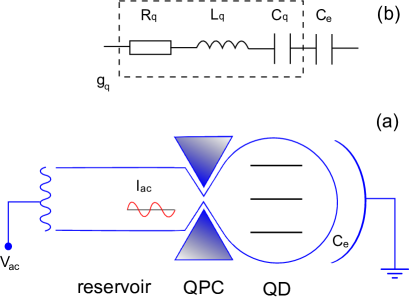
Figure 1: (Color online) (a) Mesoscopic capacitor. The tunneling between the QD and the reservoir are controlled via the QPC. An external ac field $V_{\rm ac}$ causes the carrier exchange between the QD and the reservoir, leading to an ac current $I_{\rm ac}$. The QD and the metallic electrode on the right are capacitively coupled, which does not permit carrier exchange. (b) The low-frequency equivalent circuit of the mesoscopic capacitor. The geometrical capacitance $C_{e}$ (formed between the QD and the right electrode) is in series with the quantum conductance $g_{q}$. At low frequencies, $g_{q}$ can be characterized by a quantum capacitor $C_{q}$, a charge relaxation resistance $R_{q}$ and a quantum inductance $L_{q}$.

The effect of the Wigner-Smith delay time $\tau_{W}$ on the low-frequency ac conductance can be vividly interpreted within the delayed current picture introduced by Ringel et al..ringel2008 They show that the total current of the mesoscopic capacitor can be interpreted in terms of an incoming current and an outgoing current. While the incoming current responds instantaneously to the external driving field, the outgoing current is delayed by $\tau_{W}$ with respect to the incoming one. Such picture well captures the behavior of ac conductance at low frequencies. It is worth noting that at higher frequencies, the effect of the Wigner-Smith delay time are expected to be more pronounced. Wang et al. have shown that up to the third order of the frequency, it can lead to a quantum inductance $L_{q}=R_{q}\tau_{W}/12$ under the resonance condition when the QD levels are aligned with the Fermi energy of the reservoir.wang2007 The corresponding $G(\omega)$ can be written as

$$G(\omega) = -i\omega C_{\mu}(1+i\omega R_{q}C_{\mu}-\omega^{2}C^{2}_{\mu}R^{2}_{q}+\omega^{2}C_{\mu}L_{q})$$ (2)

$$+O(\omega^{3}).$$

The above result highlights the importance of the Wigner-Smith delay time on the charge dynamics of the mesoscopic capacitor.

One may wonder whether there are other characteristic times that can also play a role on the ac conductance, especially at higher frequencies. This is the main motivation of this work. To study this question, we first reexamine the delayed current picture and find that the current delay characterized by the Wigner-Smith delay time $\tau_{W}$ can only describe the behavior of the ac conductance $G(\omega)$ up to the second order of the frequency. As the frequency goes higher, another effect —current deformation— can be important. A new characteristic time —deformation time $\tau_{S}$— is then introduced to describe such effect. While the Wigner-Smith delay time $\tau_{W}$ is decided by the density of states of the mesoscopic capacitor, the deformation time $\tau_{S}$ is related to its second-order derivative. The two characteristic times can be related via a simple relation

$$\frac{\tau^{{}^{\prime\prime}}_{W}}{\tau^{3}_{S}} = \frac{24}{\hbar^{2}}.$$ (3)

By incorporating the current deformation into the delayed current picture(which can be referred as delayed-deformed picture), we find that $\tau_{S}$ can manifest itself in the quantum inductance $L_{q}$ as

$$L_{q} = R_{q}\tau_{W}[4\big{(}\frac{\tau_{S}}{\tau_{W}}\big{)}^{3}+\frac{1}{6}].$$ (4)

Due to the effect of $\tau_{S}$, the quantum inductance $L_{q}$ can have quite different behaviors from the quantum capacitance $C_{q}$. Specifically, $L_{q}$ can exhibit dips around the resonances where $C_{q}$ exhibits peaks. The $L_{q}$ obtained by Wang et al. in Ref. wang2007, can be treated as a specific case of Eq. (4) at the resonances.

We further validate the conclusions obtained from the delayed-deformed picture by performing more realistic calculations within the non-equilibrium Green’s function (NEGF) formalism, where the effect of the charging energy in the QD and the nonzero temperature have been taken into consideration. We find that the relation between the deformation time $\tau_{S}$ and the Wigner-Smith delay time $\tau_{W}$ [Eq. (3)] is a good approximation at sufficient low temperatures despite the presence of the charging energy. As the temperature increases, such relation tends to break down and one has instead

$$\frac{\tau^{{}^{\prime\prime}}_{W}}{\tau^{3}_{S}} \to 0,$$ (5)

in the high temperature limit. We also find that the deformation time $\tau_{S}$ do have a pronounced impact on the quantum inductance $L_{q}$. It can not only lead to dips around the resonances, but also make $L_{q}$ changes its sign at nonzero temperatures: $L_{q}$ can go from positive values at low temperatures to large negative values at high temperatures. Thus, just like the universality of the charge relaxation resistance $R_{q}$, the positive definiteness of $L_{q}$ can also be regarded as a signature of the quantum coherent transport. The above results demonstrate the importance of the deformation time $\tau_{S}$ on the ac conductance of the mesoscopic capacitor.

The paper is organized as follows: In Sec. II, we generalize the delayed current picture to include the current deformation effect. In Sec. III, we present the Hamiltonian and the NEGF formalism. The numerical results from the NEGF formalism are discussed in Sec. IV. We summarized in Sec. V.

II DELAYED-DEFORMED CURRENT

In this section, we generalize the delayed current picture to include the current deformation effect.

Following the scattering formalism,blanter2000 the current operator for the single-channel mesoscopic capacitor can be decomposed into an incoming part $\hat{I}_{+}$ and outgoing part $\hat{I}_{-}$, which can be expressed as

$$\hat{I}(t) = \hat{I}_{+}(t)-\hat{I}_{-}(t),$$ (6)

$$\hat{I}_{+}(t) = \frac{e}{2\pi\hbar}\int dE\hat{n}_{+}(E,t),$$ (7)

$$\hat{I}_{-}(t) = \frac{e}{2\pi\hbar}\int dE\hat{n}_{-}(E,t),$$ (8)

where $\hat{n}_{+}$($\hat{n}_{-}$) is the operator describing the occupation numbers of the incoming(outgoing) channel. They can be written as

$$\hat{n}_{+}(E,t) = \int d\omega e^{-i\omega t}\hat{a}^{\dagger}(E-\hbar\omega/2)\hat{a}(E+\hbar\omega/2),$$ (9)

$$\hat{n}_{-}(E,t) = \int d\omega e^{-i\omega t}\hat{b}^{\dagger}(E-\hbar\omega/2)\hat{b}(E+\hbar\omega/2),$$ (10)

where $\hat{a}(E)$[$\hat{b}(E)$] and $\hat{a}^{\dagger}(E)$[$\hat{b}^{\dagger}(E)$] are the creation and annihilation operators of electrons in the incoming(outgoing) channel with energy $E$, respectively.

For the case of elastic scattering, the operators $\hat{a}$ and $\hat{b}$ are related via the scattering matrix, which can be described by just a pure phase factor $\phi$ for the single-channel system,pretre1996 ; buttiker1992 ; levinson2000

$$\hat{b}(E) = S(E)\hat{a}(E),$$ (11)

$$S(E) = e^{i\phi(E)}.$$ (12)

By substituting Eqs. (11) and (12) into Eqs. (9) and (10), one obtains the relation between the occupation number operator of incoming and outgoing electrons,

$$\hat{n}_{-}(E,t) = \int dt^{\prime}\hat{n}_{+}(E,t^{\prime})A(E,t-t^{\prime}),$$ (13)

where the effects of the scattering are attributed to the integral kernel $A(E,t)$. It can be expressed in terms of the scattering phase factor as

$$A(E,t) = \int\frac{d\omega}{2\pi}e^{-i\omega t}e^{-i[\phi(E-\hbar\omega/2)-\phi(E+\hbar\omega/2)]}.$$ (14)

If the scattering phase factor $\phi(E)$ is slow-varying with respect to the energy $E$, the integral kernel $A(E,t)$ can be expanded with respect to the frequency $\omega$, yielding the low-frequency expansion

$$A(E,t) = \int\frac{d\omega}{2\pi}e^{-i\omega t}e^{i\omega\tau_{W}+i\omega^{3}\tau^{3}_{S}+O(\omega^{3})}.$$ (15)

The two parameters $\tau_{W}$ and $\tau_{S}$ in Eq. (15) can be written as

$$\tau_{W}(E) = 2\pi\hbar\rho(E),$$ (16)

$$\tau_{S}(E) = \frac{\hbar}{2}\sqrt[3]{\frac{2\pi\rho^{\prime\prime}(E)}{3}},$$ (17)

where $\rho(E)=\rm{Tr}[S^{\dagger}\partial_{E}S]/(2\pi i)$ representing the density of states for the capacitor plate,nigg2006 while $\rho{{}^{\prime\prime}}(E)$ denoting the second-order derivative of $\rho(E)$ with respect to the energy $E$.

Equation (15) indicates that at low frequencies, the effect of the scattering can be described by the two parameters $\tau_{W}$ and $\tau_{S}$. The parameter $\tau_{W}$ is just the Wigner-Smith delay time, indicating that the due to the scattering, the outgoing current is delayed from the incoming current by $\tau_{W}$, while the profile of the outgoing current remains the same as the incoming one. The parameter $\tau_{S}$, which also has dimension of time, indicates that due to the scattering, the profile of the outgoing current is deformed from the incoming one. The magnitude of the deformation can be quantitatively described by $\tau_{S}$, hence it can be referred as ”deformation” time. It is worth emphasizing that according to Eqs. (16) and (17), the deformation time $\tau_{S}$ can be related to the Wigner-Smith delay time $\tau_{W}$ as

$$\frac{\tau^{{}^{\prime\prime}}_{W}}{\tau^{3}_{S}} = \frac{24}{\hbar^{2}}.$$ (18)

Both $\tau_{W}$ and $\tau_{S}$ can manifest itself in the quantum conductance $g_{q}$ of the mesoscopic capacitor[Fig. 1(b)]. Up to the first-order of the frequency $\omega$, only the effect of the current delay can play a role. The corresponding quantum conductance can be approximated as

$$g_{q}(\omega) \approx \frac{e^{2}}{h}(1-e^{i\omega\tau_{W}(E_{F})}),$$ (19)

with $E_{F}$ being the Fermi energy of the reservoir. This is just the result obtained within the delayed current picture.ringel2008 Up to the second-order of the frequency $\omega$, the effect of the current deformation can also be important. The quantum conductance $g_{q}$ including this effect becomes (see Appendix A for derivation)

$$g_{q}(\omega) \approx \frac{e^{2}}{h}[1-2e^{i\omega\tau_{W}(E_{F})}e^{i\omega^{3}\tau^{3}_{S}(E_{F})}$$ (20)

$$\hskip 71.13188pt+e^{i\omega\tau_{W}(E_{F})}].$$

Equation (20) demonstrates the effect of the current deformation on the charge dynamics of the mesoscopic capacitor.

As the deformation time $\tau_{S}$ does not play a role on the quantum conductance $g_{q}$ up to the first-order of the frequency, it can not affect the quantum capacitance $C_{q}$ and the relaxation resistance $R_{q}$ of the mesoscopic capacitor. However, it does have a non-negligible influence on the quantum inductance $L_{q}$. To show this, we calculate $C_{q}$, $R_{q}$ and $L_{q}$ by matching the impedance of the mesoscopic capacitorgabelli2006 ; buttiker1993 ; wang2007

$$Z(\omega) = \frac{1}{g_{q}(\omega)}-\frac{1}{i\omega C_{e}},$$ (21)

to the corresponding formula for a classical RLC circuits

$$Z(\omega) = \frac{i}{\omega}\Big{(}\frac{C_{q}C_{e}}{C_{q}+C_{e}}-i\omega R_{q}-\omega^{2}L_{q}\Big{)},$$ (22)

where the quantum conductance $g_{q}$ is given by Eq. (20). By comparing Eq. (21) to Eq. (22), one obtains

$$C_{q} = \frac{e^{2}}{h}\tau_{W},$$ (23)

$$R_{q} = \frac{h}{2e^{2}},$$ (24)

$$L_{q} = R_{q}\tau_{W}[4\big{(}\frac{\tau_{S}}{\tau_{W}}\big{)}^{3}+\frac{1}{6}].$$ (25)

The influence of the deformation time $\tau_{S}$ on the quantum inductance $L_{q}$ can be clearly seen from Eq. (25).

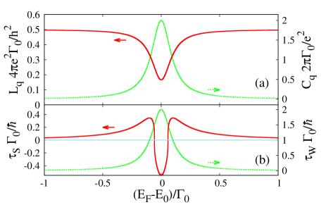
Figure 2: (Color online) (a) The quantum inductance $L_{q}$ (red solid curve) and quantum capacitance $C_{q}$ (green dotted curve) as function of the Fermi energy $E_{F}$. (b) The corresponding deformation time $\tau_{S}$ (red solid curve) and the Wigner-Smith delay time $\tau_{W}$ (green dotted curve) as function of the Fermi energy $E_{F}$. The thin skyblue line indicates the zero value for $\tau_{S}$.

Due to the additional contribution from the deformation time $\tau_{S}$, the quantum inductance $L_{q}$ can have quite different behaviors from the ones of the quantum capacitance $C_{q}$. To illustrate this, we suppose the density of states $\rho(E)$ of the mesoscopic capacitor is given by a single Lorentzian peak around $E_{0}$ with width $\Gamma_{0}$,

$$\rho(E) = \frac{1}{\pi}\frac{\Gamma_{0}}{(E-E_{0})^{2}+\Gamma^{2}_{0}},$$ (26)

then according to Eqs. (23) and (25), $C_{q}$ also exhibits a Lorentzian peak as a function of $E_{F}$, while $L_{q}$ exhibits a dip around $E_{0}$, as illustrated in Fig. 2(a). At the resonance ($E_{F}=E_{0}$) where $C_{q}$ reaches its maximum, $L_{q}$ reaches its minimum value $L^{\rm min}_{q}=R_{q}\tau^{\rm max}_{W}/12$ with $\tau^{\rm max}_{W}=2\hbar/\Gamma_{0}$. This is just the result obtained by Wang et al. in Ref. wang2007, . Far from the resonance ($|E_{F}-E_{0}|\gg\Gamma_{0}$) where $C_{q}$ tends to zero, $L_{q}$ reaches its maximum value $L^{\rm max}_{q}=3L^{\rm min}_{q}$. By comparing to the corresponding $\tau_{S}$ and $\tau_{W}$ in Fig. 2(b), one can see that the dip in $L_{q}$ can be attributed to the contribution of $\tau_{S}$, which also exhibits a dip around the resonance.

It is worth noting that the relation between $L_{q}$ and $\tau_{S}$ can offer a way to detect the detailed structure of the density of states $\rho(E)$, since $\tau_{S}$ is related to the second-order derivative of $\rho(E)$ [Eq. (17)]. It is interesting to remind that the first-order derivative of $\rho(E)$ can be accessed via the thermoelectric capacitance.lim2013 This suggests that by combining the charge and thermoelectric admittance, one can obtain more complete information of mesoscopic systems.

To summarize this section, we have generalize the delayed current picture to include the current deformation effect into consideration. Such effect can be quantitatively described by the deformation time $\tau_{S}$, which is related to the Wigner-Smith delay time via a simple relation Eq. (18). The deformation time $\tau_{S}$ can have a pronounced impact on the quantum inductance $L_{q}$ of the mesoscopic capacitor, making $L_{q}$ having quite different behaviors from the ones of the quantum capacitance $C_{q}$.

III NEGF FORMALISM

Although the delayed-deformed current picture offers a vivid interpretation of the charge dynamics of the mesoscopic capacitor, the approximation used in the derivation is rather crude. Some effects, such as the breakdown of the universality of $R_{q}$,nigg2006 are ignored in such picture. To further validate the conclusions from the delayed-deformed current picture, we perform more realistic calculations within the framework of non-equilibrium Green’s function (NEGF) formalism.

Let us first present the Hamiltonian of the mesoscopic capacitor which is illustrated in Fig. 1. It can be written asringel2008

$$H = H_{L}+H_{D}+H_{\rm LD},$$ (27)

where $H_{L}$, $H_{D}$ and $H_{\rm LD}$ describe the reservoir, the QD and their coupling, respectively. The reservoir Hamiltonian $H_{L}$ is derived from a one-dimensional tight-binding model, which can be written as

$$H_{L} = \int dk\varepsilon(k)a^{\dagger}_{k}a_{k},$$ (28)

where $\varepsilon(k)=-2t_{0}\cos(k)$ is the dispersive relation with $t_{0}$ being the hopping between adjacent sites. The Hamiltonian of the QD, including the single-particle part and interactions, can be expressed as

$$H_{D} = \sum^{n_{d}}_{n=1}\epsilon_{n}d^{\dagger}_{n}d_{n}+\frac{E_{C}}{2}(\hat{N}-\frac{n_{d}}{2})^{2},$$ (29)

where $\epsilon_{n}=n\Delta$ with $\Delta$ being the level spacing. $E_{C}=e^{2}/C_{e}$ describes the charging energy with $C_{e}$ being the geometrical capacitance. $\hat{N}=\sum^{n_{d}}_{n=1}d^{\dagger}_{n}d_{n}$ is the number operator of the electrons in the QD with $n_{d}$ devoting the number of QD levels. The coupling $H_{LD}$ can be written as

$$H_{LD} = \sum_{n}\int dk(t_{\rm kn}d^{\dagger}_{n}a_{k}+{\rm H.c.}),$$ (30)

with $t_{\rm kn}$ being the coupling matrix element.

Within the NEGF formalism, the quantum admittance $g_{q}(\omega)$ can be calculated in the wide-band-limithaugbook ; bgwang1999 ; ma1999 as

$$g_{q}(\omega) = -i\frac{e^{2}}{h}\int d\omega^{\prime}{\rm Tr}[G^{r}_{D}(\omega+\omega^{\prime})\frac{\Gamma}{\hbar}G^{a}_{D}(\omega^{\prime})]$$ (31)

$$\times[f(\omega^{\prime})-f(\omega+\omega^{\prime})],$$

where $G^{\rm r/a}_{D}(\omega)$ represents the equilibrium retarded/advanced Green function of the QD while $\Gamma$ describes the level-width function of the QD due to the coupling to the reservoir.haugbook $f(\omega)=1/[1+\exp(\beta(\hbar\omega-E_{F}))]$ represents the equilibrium electron distribution, with $E_{F}$ being the Fermi level and $\beta=1/(k_{B}T)$ being the inverse temperature. The Taylor expansion of $g_{q}(\omega)$ with respect to the frequency $\omega$ reads

$$g_{q}(\omega) = e_{0}+e_{1}\omega+e_{2}\omega^{2}+O(\omega^{3}),$$ (32)

$$e_{0} = -\int d\omega f^{\prime}(\omega){\rm Tr}[G^{r}_{D}(\omega)\frac{\Gamma}{\hbar}G^{a}_{D}(\omega)],$$ (33)

$$e_{1} = -\int d\omega\frac{f^{\prime}(\omega)}{2}{\rm Tr}[(G^{r}_{D}(\omega))^{\prime}\frac{\Gamma}{\hbar}G^{a}_{D}(\omega)$$ (34)

$$-G^{r}_{D}(\omega)\frac{\Gamma}{\hbar}(G^{a}_{D}(\omega))^{\prime}],$$

$$e_{2} = -\int d\omega\frac{f^{\prime}(\omega)}{6}{\rm Tr}[(G^{r}_{D}(\omega))^{\prime\prime}\frac{\Gamma}{\hbar}G^{a}_{D}(\omega)$$ (35)

$$+G^{r}_{D}(\omega)\frac{\Gamma}{\hbar}(G^{a}_{D}(\omega))^{\prime\prime}-(G^{r}_{D}(\omega))^{\prime}\frac{\Gamma}{\hbar}(G^{a}_{D}(\omega))^{\prime}],$$

where $(G^{r/a}_{D}(\omega))^{\prime}$ and $(G^{r/a}_{D}(\omega))^{\prime\prime}$ represent the first-order and second-order derivatives of the retarded/advanced QD Green function with respect to the frequency $\omega$.

By substituting Eqs. (32-35) into Eq. (21) and comparing to Eq. (22-25), one obtains the quantum capacitor $C_{q}$, charge relaxation resistance $R_{q}$ and the quantum inductance $L_{q}$ as

$$C_{q} = \frac{e^{2}}{h}e_{0},$$ (36)

$$R_{q} = \frac{\tau_{W}}{2C_{q}},$$ (37)

$$L_{q} = R_{q}\tau_{W}[4\big{(}\frac{\tau_{S}}{\tau_{W}}\big{)}^{3}+\frac{1}{6}],$$ (38)

where the two characteristic times $\tau_{W}$ and $\tau_{S}$ can be expressed as

$$\tau_{W} = -2i\frac{e_{1}}{e_{0}},$$ (39)

$$\tau_{S} = \sqrt[3]{\frac{5}{24}-\frac{e_{0}e_{2}}{4e^{2}_{1}}}.$$ (40)

To obtain $C_{q}$, $R_{q}$ and $L_{q}$, one needs to find the equilibrium retarded/advanced QD Green function $G^{\rm r/a}_{D}$. They can be calculated self-consistently within the Hartree-Fock approximation asringel2008 ; nigg2006

$$G^{r}_{D} = [\hbar\omega-H+\frac{i\gamma}{2}]^{-1},$$ (41)

$$H_{\rm mn} = \delta_{\rm mn}d+E_{C}\big{(}\delta_{\rm nm}\sum_{\bar{n}}Q_{\rm\bar{n}\bar{n}}-Q_{\rm nm}\big{)},$$ (42)

$$Q_{\rm mn} = -\hbar\int\frac{d\omega}{\pi}f(\omega){\rm Im}[G^{r}_{D}]_{\rm mn}.$$ (43)

In the calculation, we have assume all the QD levels coupled to the lead with the same strength, i.e., $\Gamma_{\rm mn}=\gamma$.buttiker2007 ; ringel2008 Following Refs. buttiker2007, ; brouwer1997, , we choose the coupling $\gamma$ as

$$\gamma = \frac{\Delta}{\pi D}\Big{(}2-D-2\sqrt{1-D}\Big{)},$$ (44)

where $D$ describes the probability for transmission through the QPC. It can be related to the Fermi energy $E_{F}$ in the lead asbuttiker1990

$$D = \frac{1}{1+e^{-aE_{F}/\Delta}},$$ (45)

with $a$ being a constant depends on the detail structure of the QPC potential.

IV NUMERICAL RESULTS

The computations in this section are performed for the QD with $29$ levels. The parameter $a$ of the QPC is chosen to be $1.9$. The Fermi energy $E_{F}$ and the QD charging energy $E_{C}$ are all measured in units of the QD level spacing $\Delta$.

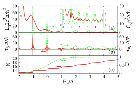
Figure 3: (Color online) (a) The quantum inductance $L_{q}$ (red solid curve) and quantum capacitance $C_{q}$ (green dashed curve) as function of the Fermi energy $E_{F}$. The zoom of $L_{q}$ and $C_{q}$ in the region $E_{F}/\Delta\in[0,5]$ are plotted in the inset. (b) The deformation time $\tau_{S}$ (red solid curve) and the Wigner-Smith delay time $\tau_{W}$ (green dashed curve) as function of the Fermi energy $E_{F}$. The thin black line indicates the zero value. (c) The total dot charge $N$ of the QD (red solid curve) and the transmission probability $D$ through the QPC (green dashed curve) as function of the Fermi energy. In all the figures, the temperature is set to $0$ K and the charging energy $E_{C}$ is set to $0$.

We start the discussion from the simplest case where the temperature $T=0$ K and the charging energy $E_{C}=0$.comment1 Let us first compare the behaviors of the quantum inductance $L_{q}$ and the quantum capacitance $C_{q}$. The $L_{q}$ and $C_{q}$ as function of the Fermi energy $E_{F}$ are plotted in Fig. 3(a). The corresponding Wigner-Smith delay time $\tau_{W}$ and deformation time $\tau_{S}$ are plotted in Fig. 3(b). We also plot the total dot charge $N$ and the probability for transmission through the QPC $D$ in Fig. 3(c) for comparison. From the figure, one can see that although both $L_{q}$ and $C_{q}$ exhibit distinct oscillations as $E_{F}$ varies, the detail structure of these oscillations are different. For small $E_{F}$ where the QPC is close to pinch-off ($D\ll 1$), $C_{q}$ exhibits single sharp peaks at the resonances where the transfer of an electron into the QD is permitted. For large $E_{F}$ where the QPC is opened ($D\rightarrow 1$), the peak is broadened and its height is decreased. On the contrary, $L_{q}$ exhibits sharp dips at the resonances when the QPC is close to pinch-off, with two shoulder peaks appearing at both sides of the dip. As the QPC is opened, such dip-double-peak structures are suppressed into smooth shallow valleys.

By comparing to the corresponding $\tau_{S}$ and $\tau_{W}$, one can see that the behavior of $C_{q}$ is solely decided by $\tau_{W}$, while the dip-double-peak structures in $L_{q}$ can be attributed to the contribution from $\tau_{S}$. Hence one concludes that the deformation time $\tau_{S}$ does play an important role on the quantum inductance $L_{q}$. It can make $L_{q}$ exhibiting dips around the resonances. These conclusions agree with the interpretation of the delayed-deformed current picture Given in Sec. II.

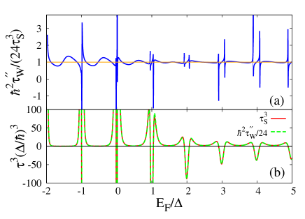
Figure 4: (Color online) (a) The ratio $\hbar^{2}\tau^{{}^{\prime\prime}}_{W}/(24\tau^{3}_{S})$ as a function of $E_{F}$. The thin orange line indicates the value $1$. (b) The quantities $\tau^{3}_{S}$ (red solid curve) and $\hbar^{2}\tau^{{}^{\prime\prime}}_{W}/24$ (green dashed curve) as function of $E_{F}$. They are measured in units of $(\Delta/\hbar)^{3}$. The thin black line indicates the value $0$. In both figures, the temperature is set to $0$ K and the charging energy $E_{C}$ is set to $0$.

Now let us discuss the relation between $\tau_{W}$ and $\tau_{S}$. The delayed-deformed current picture predicts that they can be related via Eq. (18). To check this, we plot the ratio $\hbar^{2}\tau^{{}^{\prime\prime}}_{W}/(24\tau^{3}_{S})$ as a function of $E_{F}$ in Fig. 4(a). From the figure, one can see that the ratio $\hbar^{2}\tau^{{}^{\prime\prime}}_{W}/(24\tau^{3}_{S})$ is not exactly equal but quite close to the value $1$. Relative large deviations occur only in the vicinity of the resonances. However, the deviations are modest and the two quantities $\tau^{3}_{S}$ and $\hbar^{2}\tau^{{}^{\prime\prime}}_{W}/24$ agree quite well, as can be seen from Fig. 4(b). This indicates that although the relation Eq. (18) derived from the delayed-deformed picture is not exact, it can be regarded as a good approximation.

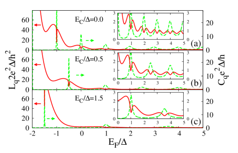
Figure 5: (Color online) The quantum inductance $L_{q}$ and quantum capacitance $C_{q}$ as function of the Fermi energy $E_{F}$ for $E_{C}/\Delta=0.0$ (a), $E_{C}/\Delta=0.5$ (b) and $E_{C}/\Delta=1.5$ (c). The zooms of $L_{q}$ and $C_{q}$ in the region $E_{F}/\Delta\in[0,5]$ are plotted in the insets. In all the figures, the temperature is set to $0$ K.

Next we turn to study the effect of the charging energy $E_{C}$. In Fig. 5, we plot the zero-temperature $L_{q}$ and $C_{q}$ as function of the Fermi energy $E_{F}$ with different charging energy $E_{C}$. From the figure, one can still identify the dip-double-peak structures in $L_{q}$ around the resonances, even for nonzero charging energy $E_{C}$. Note that as $E_{C}$ increases, the dip-double-peak structures tend to be smeared out, making the oscillations in $L_{q}$ less pronounced. This is similar to the suppression of oscillations in $C_{q}$, which has been reported in previous works.ringel2008 ; matveev1995

Figure 6: (Color online) The quantities $\tau^{3}_{S}$ (red solid curve) and $\hbar^{2}\tau^{{}^{\prime\prime}}_{W}/24$ (green dashed curve) as function of $E_{F}$ for $E_{C}/\Delta=0.0$ (a), $E_{C}/\Delta=0.5$ (b) and $E_{C}/\Delta=1.5$ (c). They are measured in units of $(\Delta/\hbar)^{3}$. The thin black lines indicate the value $0$. The corresponding ratios $\hbar^{2}\tau^{{}^{\prime\prime}}_{W}/(24\tau^{3}_{S})$ are plotted in (d), (e) and (f), respectively. The thin orange lines indicate the value $1$. In all the figures, the temperature is set to $0$ K.

The corresponding ratio $\hbar^{2}\tau^{{}^{\prime\prime}}_{W}/(24\tau^{3}_{S})$ are plotted in Fig. 6(d-f). One can see that for large $E_{F}$ when the QPC is opened, the ratio is still quite close to $1$ and is not sensitive to $E_{C}$. For small $E_{F}$ when the QPC is close to pinch-off, the ratio is relatively sensitive and it can deviate from the value $1$ as $E_{C}$ increases. However, the deviation is still small since the two quantities $\tau^{3}_{S}$ and $\hbar^{2}\tau^{{}^{\prime\prime}}_{W}/24$ agree quite well, as can be seen from Fig. 6(a-c). This indicates that the relation between $\tau_{W}$ and $\tau_{S}$ given by Eq. (18) is still a good approximation for nonzero charging energy $E_{C}$, especially for the cases with large $E_{F}$ when the QPC is opened.

The previous results justify the conclusions obtained from the delayed-deformed picture: (1) The deformation time $\tau_{S}$ can play an important role on the quantum inductance $L_{q}$, leading to dips around the resonances. (2) The deformation time $\tau_{S}$ can be approximated from the Wigner-Smith delay time $\tau_{W}$ via the simple relation Eq. (18). These conclusions hold at zero temperature, despite the presence of the charging energy.

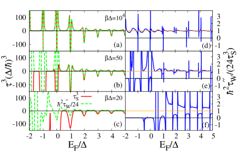
Figure 7: (Color online) The quantities $\tau^{3}_{S}$ (red solid curve) and $\hbar^{2}\tau^{{}^{\prime\prime}}_{W}/24$ (green dashed curve) as function of $E_{F}$ at inverse temperature $\beta\Delta=10^{4}$ (a), $\beta\Delta=50$ (b) and $\beta\Delta=20$ (c). The thin black lines in (a-c) indicate the zero value. The corresponding ratios $\hbar^{2}\tau^{{}^{\prime\prime}}_{W}/(24\tau^{3}_{S})$ are plotted in (d), (e) and (f), respectively. The thin black lines in (d-f) indicate the zero value, while the thin orange lines represent the value $1$. In all the figures, the charging energy $E_{C}$ is set to $0$.

It is then natural to ask what happens to the quantum inductance $L_{q}$ and deformation time $\tau_{S}$ at nonzero temperatures. To study this, we first concentrate on the quantities $\tau^{3}_{S}$ and $\hbar^{2}\tau^{{}^{\prime\prime}}_{W}/24$ as function of $E_{F}$ at different temperatures without the charging energy $E_{C}$ in Fig. 7(a-c). The corresponding ratio $\hbar^{2}\tau^{{}^{\prime\prime}}_{W}/(24\tau^{3}_{S})$ are also plotted in Fig. 7(d-f). From the figure, one can see that at high temperatures, the quantity $\tau^{3}_{S}$ (red solid curve) disagrees with $\hbar^{2}\tau^{{}^{\prime\prime}}_{W}/24$ (green dashed curve). Accordingly, the corresponding ratio $\hbar^{2}\tau^{{}^{\prime\prime}}_{W}/(24\tau^{3}_{S})$ tends to go from the value $1$ at low temperatures to the value $0$ at high temperatures. Such effect is more pronounced in the small $E_{F}$ region where the QPC is close to pinch-off. It is worth noting that the increasing of the temperature can induce an overall decreasing of the quantity $\tau^{3}_{S}$, making $\tau^{3}_{S}$ become large negative values at high temperatures.

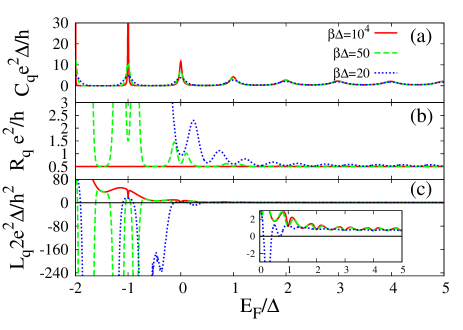
Figure 8: (Color online) The quantum capacitance $C_{q}$ (a) , charge relation resistance $R_{q}$ (b) and quantum inductance $L_{q}$ (c) as function of Fermi energy $E_{F}$ at different inverse temperatures. The zooms of $L_{q}$ in the region $E_{F}/\Delta\in[0,5]$ are plotted in the insets of (c). The thin black lines in (c) and the inset indicate the zero value. In all the figures, the charging energy $E_{C}$ is set to $0$.

The large negative $\tau_{S}$ can have a pronounced influence on the quantum inductance $L_{q}$, leading to quite different behaviors from the ones in the zero temperature limit. This is illustrated in Fig. 8. From the figure, one can see that $L_{q}$ can go from positive to negative in the region $E_{F}/\Delta<0.73$ as the temperature increases. Note that in the corresponding region, the oscillations in $C_{q}$ are largely suppressed, while $R_{q}$ deviates from the universal value $e^{2}/(2h)$, which are attributed to the breaking of the quantum coherence.gabelli2006 ; nigg2006

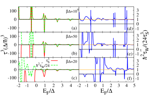
Figure 9: (Color online) The quantities $\tau^{3}_{S}$ (red solid curve) and $\hbar^{2}\tau^{{}^{\prime\prime}}_{W}/24$ (green dashed curve) as function of $E_{F}$ with inverse temperature $\beta\Delta=10^{4}$ (a), $\beta\Delta=50$ (b) and $\beta\Delta=20$ (c). The thin black lines in (a-c) indicate the zero value. The corresponding ratios $\hbar^{2}\tau^{{}^{\prime\prime}}_{W}/(24\tau^{3}_{S})$ are plotted in (d), (e) and (f), respectively. The thin black lines in (d-f) indicate the zero value, while the thin orange lines represent the value $1$. In all the figures, the charging energy $E_{C}$ is set to $0.5$.

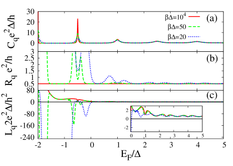
Figure 10: (Color online) The quantum capacitance $C_{q}$ (a) , charge relation resistance $R_{q}$ (b) and quantum inductance $L_{q}$ (c) as function of Fermi energy $E_{F}$ at different temperatures. The zooms of $L_{q}$ in the region $E_{F}/\Delta\in[0,5]$ are plotted in the insets of (c). The thin black lines in (c) and the inset indicate the zero value. In all the figures, the charging energy $E_{C}$ is set to $0.5$.

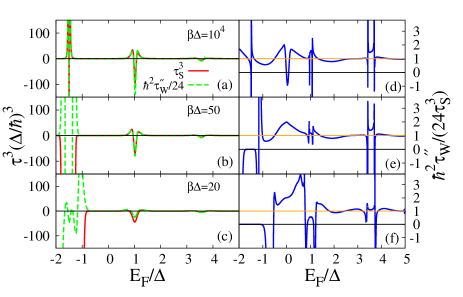
Figure 11: (Color online) The quantities $\tau^{3}_{S}$ (red solid curve) and $\hbar^{2}\tau^{{}^{\prime\prime}}_{W}/24$ (green dashed curve) as function of $E_{F}$ with inverse temperature $\beta\Delta=10^{4}$ (a), $\beta\Delta=50$ (b) and $\beta\Delta=20$ (c). The thin black lines in (a-c) indicate the zero value. The corresponding ratios $\hbar^{2}\tau^{{}^{\prime\prime}}_{W}/(24\tau^{3}_{S})$ are plotted in (d), (e) and (f), respectively. The thin black lines in (d-f) indicate the zero value, while the thin orange lines represent the value $1$. In all the figures, the charging energy $E_{C}$ is set to $1.5$.

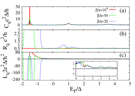
Figure 12: (Color online) The quantum capacitance $C_{q}$ (a) , charge relation resistance $R_{q}$ (b) and quantum inductance $L_{q}$ (c) as function of Fermi energy $E_{F}$ at different temperatures. The zooms of $L_{q}$ in the region $E_{F}/\Delta\in[0,5]$ are plotted in the insets of (c). The thin black lines in (c) and the inset indicate the zero value. In all the figures, the charging energy $E_{C}$ is set to $1.5$.

In the presence of charging energy $E_{C}$, one can also find similar high temperature behaviors of $\tau_{S}$ and $L_{q}$, which can be seen by comparing Fig. 7[Fig. 8] to Fig. 9[Fig. 10] for $E_{C}/\Delta=0.5$ and to Fig. 11[Fig. 12] for $E_{C}/\Delta=1.5$. Note that as $E_{C}$ increases, the effect of the nonzero temperature is less and less pronounced.

According to the previous discussion, one can conclude that as the temperature increases, the ratio $\hbar^{2}\tau^{{}^{\prime\prime}}_{W}/(24\tau^{3}_{S})$ goes from the value $1$ at low temperatures to $0$ at high temperatures. Accordingly, the quantum inductance $L_{q}$ also show different behavior at high temperatures: It can go from positive values at low temperatures to large negative values at high temperatures. Hence, the relation $\hbar^{2}\tau^{{}^{\prime\prime}}_{W}/(24\tau^{3}_{S})\approx 1$ and the positive definiteness of $L_{q}$ can be regarded as signatures of the ac quantum coherent transport.

V SUMMARY

In this work, we have examined the characteristic times which describe the low frequency dynamics of the mesoscopic capacitors. By combining the delayed-deformed current picture and the numerical calculations within NEGF formalism, we found that the Wigner-Smith delay time $\tau_{W}$ can only capture the ac response of the mesoscopic capacitor up to the second order of the frequency. At higher frequencies, a new time scale —the deformation time $\tau_{S}$— has to be taken into consideration. The deformation time indicates that due to the scattering, the profile of the outgoing current from the dot is distorted from the incoming one. At sufficient low temperatures when the charge transport is phase-coherent, $\tau_{S}$ can be approximated from the Wigner-Smith delay time $\tau_{W}$ via a simple relation $\tau^{\prime\prime}_{W}/\tau^{3}_{S}=24/\hbar^{2}$. At high temperatures when the coherence is broken, one has instead $\tau^{\prime\prime}_{W}/\tau^{3}_{S}\to 0$. Hence this relation can be regarded as a signature of the ac quantum coherent transport. We further show that the deformation time $\tau_{S}$ can have a pronounced influence on the quantum inductance $L_{q}$ of the mesoscopic capacitor, making $L_{q}$ show quite different behaviors from the ones of the quantum capacitor $C_{q}$. The most striking one is that $L_{q}$ can change its sign as the temperature increases: It goes from positive values at low temperatures to large negative values at high temperatures. Thus the positive definiteness of $L_{q}$ can also be regarded as a signature of the ac quantum coherent transport. These results highlight the importance of the deformation time on the ac response of the mesoscopic capacitors.

*

Appendix A Derivation of Eq. (20)

We start from the expression of the quantum conductancebuttiker1993 ; buttiker1993-1 ; buttiker1994

$$g_{q}(\omega) = \frac{e^{2}}{h}\int dE[1-S^{\dagger}(E-\frac{\hbar\omega}{2})S(E+\frac{\hbar\omega}{2})]$$ (46)

$$\hskip 28.45274pt\times\frac{f(E-\frac{\hbar\omega}{2})-f(E+\frac{\hbar\omega}{2})}{\hbar\omega},$$

where $S(E)=e^{i\phi(E)}$ [Eq. (12)]. By performing a Taylor expansion with respect to $\omega$, one obtains

$$g_{q}(\omega) = \frac{e^{2}}{h}\int dE[-f^{\prime}(E)-(\frac{\hbar\omega}{2})^{2}\frac{f^{\prime\prime\prime}(E)}{6}]$$ (47)

$$+\frac{e^{2}}{h}\int dEf^{\prime}(E)e^{i\omega\tau_{W}(E)+i\omega^{3}\tau^{3}_{S}(E)}$$

$$+\frac{e^{2}}{h}\int dE(\frac{\hbar\omega}{2})^{2}\frac{f^{\prime\prime\prime}(E)}{6}e^{i\omega\tau_{W}(E)}$$

$$+O(\omega^{3}).$$

At sufficient low temperatures, the Fermi distribution $f(E)$ can be well approximated by the step function $\theta(E_{F}-E)$. By perform the integration over $E$, one has

$$g_{q}(\omega) = \frac{e^{2}}{h}$$ (48)

$${}-\frac{e^{2}}{h}e^{i\omega\tau_{W}(E_{F})+i\omega^{3}\tau^{3}_{S}(E_{F})}$$

$${}-\frac{e^{2}}{h}i\omega^{3}\frac{\hbar^{2}\tau^{\prime\prime}_{W}(E_{F})}{24}e^{i\omega\tau_{W}(E_{F})}$$

$${}+O(\omega^{3}).$$

By using the relation Eq. (18), up to the second order of the frequency $\omega$, the above equation can be approximated as

$$g_{q}(\omega) \approx \frac{e^{2}}{h}[1-2e^{i\omega\tau_{W}(E_{F})}e^{i\omega^{3}\tau^{3}_{S}(E_{F})}$$ (49)

$$\hskip 71.13188pt+e^{i\omega\tau_{W}(E_{F})}],$$

which is just the result given in Eq. (20).

References

- (1) J. Gabelli, J.-M. Berroir, G. Féve, B. Plaçais, Y. Jin, B. Etienne, and D. C. Glattli, Science 313, 499 (2006).
- (2) J. Gabelli, G. Féve, T. Kontos, J.-M. Berroir, B. Plaçais, D. C. Glattli, B. Etienne, Y. Jin, and M. Büttiker, Phys. Rev. Lett. 98, 166806 (2007).
- (3) G. Fève, A. Mahè, J.-M. Berroir, T. Kontos, B. Plaçais, D. C. Glattli, A. Cavanna, B. Etienne, and Y. Jin, Science 316, 5828 (2007).
- (4) E. Bocquillon, V. Freulon, J.-M. Berroir, P. Degiovanni, B. Plaçais, A. Cavanna, Y. Jin, and G. Féve, Science 339, 1054 (2013).
- (5) J. Dubois, T. Jullien, P. Roulleau, F. Portier, P. Roche, A. Cavanna, Y. Jin, W. Wegschneider, and D. C. Glattli, Nature 502, 659 (2013).
- (6) J. Gabelli, G. Fève, J.-M. Berroir, and B. Plaçais, Rep. Prog. Phys. 75, 126504 (2012).
- (7) A. Mahè, F. D. Parmentier, E. Bocquillon, J.-M. Berroir, D. C. Glattli, T. Kontos, B. Plaçais, G. Fève, A. Cavanna, and Y. Jin, Phys. Rev. B 82, 201309 (2010).
- (8) F. D. Parmentier, E. Bocquillon, J.-M. Berroir, D. C. Glattli, B. Plaçais, G. Fève, M. Albert, C. Flindt, and M. Büttiker, Phys. Rev. B 85, 165438 (2012).
- (9) E. Bocquillon, F. D. Parmentier, C. Grenier, J.-M. Berroir, P. Degiovanni, D. C. Glattli, B. Plaçais, A. Cavanna, Y. Jin, and G. Féve, Phys. Rev. Lett. 108, 196803 (2012).
- (10) M. Büttiker, H. Thomas, and A. Prêtre, Phys. Lett. A 180, 364 (1993).
- (11) M. Büttiker, J. Phys.: Condens. Matter 5, 9361 (1993).
- (12) M. Büttiker and S. E. Nigg, Nanotechnology 18, 044029 (2007).
- (13) S. E. Nigg, R. López, and M. Büttiker, Phys. Rev. Lett. 97, 206804 (2006).
- (14) S. E. Nigg and M. Büttiker, Phys. Rev. B 77, 085312 (2008).
- (15) M. Moskalets, P. Samuelsson, and M. Büttiker, Phys. Rev. Lett. 100, 086601 (2008).
- (16) Z. Ringel, Y. Imry, and O. Entin-Wohlman, Phys. Rev. B 78, 165304 (2008).
- (17) S. E. Nigg and M. Büttiker, Phys. Rev. Lett. 102, 236801 (2009).
- (18) C. More and K. Le Hur, Nat. Phys. 6, 697 (2010).
- (19) Y. Hamamoto, T. Jonckheere, T. Kato, and T. Martin, Phys. Rev. B 81, 153305 (2010).
- (20) M. Lee, R. López, M.-S. Choi, T. Jonckheere, and T. Martin, Phys. Rev. B 83, 201304(R) (2011).
- (21) M. Filippone and C. Mora, Phys. Rev. Lett. 86, 125311 (2012).
- (22) J. Wang, B. G. Wang, and H. Guo, Phys. Rev. B 75, 155336 (2007).
- (23) Y. M. Blanter and M. Büttiker, Phys. Rep. 336, 1 (2000).
- (24) A. Prêtre, H. Thomas, and M. Büttiker, Phys. Rev. B 54, 8130 (1996).
- (25) M. Büttiker, Phys. Rev. B 45, 3807 (1992); ibid. 46, 12485 (1992).
- (26) Y. Levinson, Phys. Rev. B 61, 4748 (2000).
- (27) J. S. Lim, R. López, and D. Sánchez, Phys. Rev. B 88, 201304(R) (2013).
- (28) H. Haug and A.-P. Jauho, Quantum Kinetics in Transport and Optics of Semiconductors (Springer-Verlag, Berlin, 1996).
- (29) B. G. Wang, J. Wang, and H. Guo, Phys. Rev. Lett. 82, 398 (1999).
- (30) Z. S. Ma, J. Wang, and H. Guo, Phys. Rev. B 59, 7575 (1999).
- (31) P. W. Brouwer and C. W. J. Beenakker, Phys. Rev. B 55, 4695 (1997).
- (32) M. Büttiker, Phys. Rev. B 41, 7906 (1990).
- (33) In the numerical calculation, we choose to describe the zero-temperature limit.
- (34) K. A. Matveev, Phys. Rev. B 51, 1743 (1995).
- (35) M. Büttiker, A. Prêtre, and H. Thomas, Phys. Rev. Lett. 70, 4114 (1993); Z. Phys. B 94, 133 (1994).