Finite-volume Hamiltonian method for coupled channel interactions in lattice QCD

Abstract

Within a multi-channel formulation of $\pi\pi$ scattering, we investigate the use of the finite-volume Hamiltonian approach to resolve scattering observables from lattice QCD spectra. The asymptotic matching of the well-known Lüscher formalism encodes a unique finite-volume spectrum. Nevertheless, in many practical situations, such as coupled-channel systems, it is advantageous to interpolate isolated lattice spectra in order to extract physical scattering parameters. Here we study the use of the Hamiltonian framework as a parameterisation that can be fit directly to lattice spectra. We find that with a modest amount of lattice data, the scattering parameters can be reproduced rather well, with only a minor degree of model dependence.

I Introduction

Lattice QCD studies are making tremendous progress in resolving the excitation spectrum of QCD Dudek:2011tt ; Edwards:2011jj ; Menadue:2011pd ; Mahbub:2012ri ; Dudek:2012xn . By the nature of the finite-volume and Euclidean time aspects of the lattice formulation, it is impossible to directly simulate scattering processes. The established way to extract of scattering information from lattice simulations is the Lüscher method Luscher:1986pf ; Luscher:1990ux . For the case of elastic 2-body scattering, Lüscher identified that the finite volume eigenstates are uniquely determined in terms of the on-shell scattering parameters (up to exponentially suppressed corrections associated with quantum fluctuations of the lightest degrees of freedom in the system). While the spectrum is determined uniquely, there are technical challenges associated with inverting a given lattice spectrum to determine scattering observables. One of these issues arises from the fact that the full rotational group is broken down by the geometry of the lattice boundary conditions. As a consequence, partial wave mixing is unavoidable in lattice simulations and eigenstates on the finite volume do not correspond to definite eigenstates of the continuum rotation group. There has been significant work in previous years addressing this issue, eg. Refs. Doring:2011nd ; Dudek:2012gj ; Doring:2012eu ; Dudek:2012xn ; Briceno:2013bda .

In the present work, we focus our attention of the study of inelastic scattering channels. The generalisation of the Lüscher formalism to incorporate inelastic channels was developed by He, Feng and Liu He:2005ey , and continues to be the topic of considerable further investigations and extensions Lage:2009zv ; Bernard:2010fp ; MartinezTorres:2011pr ; Doring:2011nd ; Hansen:2012tf ; Briceno:2012yi ; Doring:2012eu ; Li:2012bi ; Guo:2012hv ; Briceno:2013bda . In addition to the issue of partial wave mixing, coupled-channel systems are further complicated by the multi-component nature of the $S$-matrix. For example, neglecting the angular momentum mixing, for the case of two coupled channels on a given volume, a single energy eigenstate is related to three asymptotic scattering parameters (i.e. two phase shifts and an inelasticity). Therefore the only way to uniquely identify all three parameters would be to search for near- coincident energy eigenstates at either different volumes or with different momentum boosts of the system Guo:2012hv . In practice, such a “pointwise” extraction is only anticipated to have limited applicability. Alternatively, one requires some form of interpolation which can reproduce the scattering parameters with a limited set of lattice simulation results. In the present work, we extend a recently developed finite-volume Hamiltonian formalism Hall:2013qba to a coupled-channel system. The necessary equivalence with the Lüscher formalism is numerically established. Further, we investigate the inversion problem of extracting the phase shifts and inelasticity from a finite set of pseudo lattice data. We find that all three scattering parameters can be reliably reproduced by directly constraining the parameters of the model to the finite volume spectra. In the energy region constrained by the fits, the extracted phase shifts and inelasticity show only a mild sensitivity to the precise form of the model.

To facilitate the exploration of LQCD spectra, our analysis is based upon a two-channel Hamiltonian formulation which is constructed by fitting the available $\pi\pi$ scattering phase shifts data in the $J^{IP}=0^{0+},1^{1-}$ partial waves. The explicit channels included are $\pi\pi$ and the inelasticity associated with $K\bar{K}$ production. With the present manuscript being focussed primarily on the influence of the inelastic channel, we do not consider the issues associated with angular momentum mixing.

In section II, we write down a multi-channel formulation for constructing several model Hamiltonians from fitting the $\pi\pi$ scattering data. The model with only the $\pi\pi$ channel is used in section III to recall the finite-box Hamiltonian method developed in Ref. Hall:2013qba and to examine the correspondence with Lüscher’s formula. In section IV, we use the model with $\pi\pi$ and $K\bar{K}$ channels to show that the finite-box Hamiltonian approach is equivalent to the approach based on the two-channel Lüscher’s method developed in Ref. He:2005ey . In section IV, we compare the LQCD efforts needed to apply the finite-box Hamiltonian approach and the approach based on Lüscher’s method. Our predictions of the spectra for testing LQCD results for $\pi\pi$ scattering in the $J^{IP}=0^{0+},1^{1-}$ partial waves are presented in section V. In section VI, we give a summary and discuss possible future developments.

II Model Hamiltonian for $\pi\pi$ scattering

The Hamiltonian with only vertex interactions, such as $\Delta\leftrightarrow\pi N$ considered in Ref.Hall:2013qba , is the simplest example within the general multi-channel formulation, inspired by the cloudy bag model  Theberge:1980ye ; Thomas:1982kv and developed in Ref. Matsuyama:2006rp for investigating the nucleon resonances Kamano:2013iva and meson resonances Kamano:2011ih . For investigating the finite-box Hamiltonian approach in this work, it is useful to recall the formulation of Refs. Matsuyama:2006rp ; Kamano:2011ih in order to write down a general Hamiltonian for $\pi\pi$ scattering.

Following Refs. Matsuyama:2006rp ; Kamano:2011ih , we assume that $\pi\pi$ scattering can be described by vertex interactions and two-body potentials. In the rest frame, the model Hamiltonian of a meson-meson system takes the following energy-independent form

$$H=H_{0}+H_{I}.$$ (1)

The non-interacting part is

$$H_{0}=\sum_{i=1,n}|\sigma_{i}\rangle m^{0}_{i}\langle\sigma_{i}|+\sum_{\alpha}\int d\vec{k}|\alpha(\vec{k})\rangle[\sqrt{m_{\alpha_{1}}^{2}+\vec{k}^{\,\,2}_{\alpha_{1}}}+\sqrt{m_{\alpha_{2}}^{2}+\vec{k}^{\,\,2}_{\alpha_{2}}}]\langle\alpha(\vec{k})|,$$ (2)

where $\sigma_{i}$ is the $i$-th bare particle with mass $m^{0}_{i}$, $\alpha=\pi\pi,K\bar{K},\pi\eta,\cdot\cdot$ denotes the channels included, and $m_{\alpha_{i}}$ and $\vec{k}_{\alpha_{i}}$ are the mass and the momentum of the $i$-th particle in the channel $\alpha$, respectively. In the considered center of mass system, we obviously have defined $\vec{k}_{\alpha_{1}}=-\vec{k}_{\alpha_{2}}=\vec{k}$.

The interaction Hamiltonian is

$$H_{I}=g+v,$$ (3)

where $g$ is a vertex interaction describing the decays of the bare particles into two-particle channels $\alpha,\beta,\ldots$

$$g=\sum_{\alpha}\int d\vec{k}\sum_{i=1,n}\{|\alpha(\vec{k})\rangle g^{\dagger}_{i,\alpha}(k)\langle i|+|i\rangle g_{i,\alpha}(k)\langle\alpha(\vec{k})|\}$$ (4)

and the direct two-particle-two-particle interaction is defined by

$$v=\sum_{\alpha,\beta}\int d\vec{k}d\vec{k}^{\prime}\,|\alpha(\vec{k})\rangle v_{\alpha,\beta}(k,k^{\prime})\langle\beta(\vec{k}^{\prime})|.$$ (5)

In each partial wave, the two particle scattering is then defined by the following coupled-channel equations

$$t_{\alpha,\beta}(k,k^{\prime};E) =V_{\alpha,\beta}(k,k^{\prime})$$

$$\quad+\sum_{\gamma}\int_{0}^{\infty}k^{{}^{\prime\prime}\,\,2}dk^{{}^{\prime\prime}}V_{\alpha,\gamma}(k,k^{\prime\prime})\frac{1}{E-E_{\gamma_{1}}(k^{{}^{\prime\prime}})-E_{\gamma_{2}}(k^{{}^{\prime\prime}})+i\epsilon}t_{\gamma,\beta}(k^{{}^{\prime\prime}},k^{\prime};E)$$ (6)

where $E_{\gamma i}=\sqrt{k^{{}^{\prime\prime}\,\,2}+m^{2}_{\gamma_{i}}}$, and the coupled-channel potentials are

$$V_{\alpha,\beta}(k,k^{\prime})=\sum_{i=1,n}g^{*}_{i,\alpha}(k)\frac{1}{E-m_{i}^{0}}g_{i,\alpha}(k^{\prime})+v_{\alpha,\beta}(k,k^{\prime})$$ (7)

with

$$g_{i,\alpha}(k) = \langle i|g|\alpha(\vec{k})\rangle$$ (8)

$$v_{\alpha,\beta}(k,k^{\prime}) = \langle\alpha(\vec{k})|v|\beta(\vec{k}^{\prime})\rangle$$ (9)

We choose the normalization, $\langle\alpha(\vec{k})|\beta(\vec{k}^{\,\,{}^{\prime}})\rangle=\delta_{\alpha,\beta}\delta(\vec{k}-\vec{k}^{\,\,{}^{\prime}})$ such that the S-matrix in each partial-wave is related to the T-matrix by

$$S_{\alpha,\beta}(E)=1+2iT_{\alpha,\beta}(k_{0\alpha},k_{0\beta};E)$$ (10)

with

$$T_{\alpha,\beta}(k_{0\alpha},k_{0\beta};E)=-\rho^{1/2}_{\alpha}(k_{0\alpha})t_{\alpha,\beta}(k_{0\alpha},k_{0\beta};E)\rho^{1/2}_{\beta}(k_{0\beta})$$ (11)

where $k_{0\alpha}$ is the on-shell momentum for the channel $\alpha$ and the density of states is

$$\rho_{\alpha}(k_{0\alpha})=\pi\frac{k_{0\alpha}E_{\alpha 1}(k_{0\alpha})E_{\alpha 2}(k_{0\alpha})}{E_{\alpha 1}(k_{0\alpha})+E_{\alpha 2}(k_{0\alpha})}$$ (12)

In the following sections, we construct (1) one-bare state and one-channel ($1b-1c$) models, (2) one-bare state and two-channels ($1b-2c$) models, and also (3) two-bare states and two-channels ($2b-2c$) models.

III one bare state and one-channel

In this section, we consider a model which has one bare state ($\sigma$) and one-channel ($\pi\pi$) to describe the isoscalar $s$-wave $\pi\pi$ scattering phase shifts up to the energy below the $K\bar{K}$ threshold. The formulae for constructing this model, called $1b-1c$ model, can be obtained from taking $n=1$ and $\alpha=\beta=\gamma=\pi\pi$ in section II.

III.1 Model parameters

For simplicity, we parametrize the matrix elements of the interactions in Eqs.(4) and (5) as

$$\langle\sigma|g|\pi\pi(\vec{k})\rangle = g_{\sigma,\pi\pi}(k)$$ (13)

$$= \frac{g_{\pi\pi}}{\sqrt{\pi}}\frac{1}{(1+(c_{\pi\pi}\times k)^{2})},$$

$$\langle\pi\pi(\vec{k})|v|\pi\pi(\vec{k}^{\prime})\rangle = v_{\pi\pi,\pi\pi}(k,k^{\prime})$$ (14)

$$= \frac{G_{\pi\pi,\;\pi\pi}}{m^{2}_{\pi}}\times\frac{1}{(1+(d_{\pi\pi}\times k)^{2})^{2}}\times\frac{1}{(1+(d_{\pi\pi}\times k^{\prime})^{2})^{2}},$$

where $k$ and $k^{\prime}$ are the three momenta of $\pi$ in the center of mass system. By fitting the $\pi\pi$ phase shifts, the parameters, $m_{\sigma}$, $g_{\pi\pi}$, $c_{\pi\pi}$, $G_{\pi\pi,\;\pi\pi}$ and $d_{\pi\pi}$, of the model can be determined and are listed in the column “1b-1c” in Table 1. The calculated phase shifts are compared with the data in Fig. 1. The model gives a reasonable description of the data and is sufficient for exploring the systematics of the finite-volume Hamiltonian method.

Figure 1: The phase shifts of $\pi\pi$ scattering from the Model 1b-1c (cf. Table 1) are compared with the data.

Table 1: The parameters for the 1 bare state and 1 channel ($1b-1c$) model, and the 1 bare state and 2 channel ($1b-2c$) model

	1b-1c		1b-2c
$m_{\sigma}$(MeV)	700.		$700.00$
$g_{\sigma\pi\pi}$	1.6380		$2.0000$
$c_{\sigma\pi\pi}$(fm)	1.0200		$0.6722$
$G_{\pi\pi,\;\pi\pi}$	0.5560		$2.4998$
$d_{\pi\pi}$(fm)	0.5140		$0.2440$
$g_{\sigma K\bar{K}}$	-		$0.6451$
$c_{\sigma K\bar{K}}$(fm)	-		$1.0398$
$G_{K\bar{K},\;K\bar{K}}$	-		$0.0200$
$d_{K\bar{K}}$(fm)	-		$0.1000$
$G_{\pi\pi,\;K\bar{K}}$	-		$0.3500$

III.2 Finite-volume Hamiltonian

The finite-volume Hamiltonian method provides direct access to the multi-particle energy eigenstates in a periodic volume characterised by side length $L$. The quantised three momenta of the $\pi$ meson must be $k_{n}=\sqrt{n}\frac{2\pi}{L}$ for integers $n=0,1,2,\ldots$. For a given choice of $N$ momenta $(k_{0},k_{1},\ldots,k_{N-1})$, solving the Schrodinger equation $H|\Psi_{E}\rangle=E|\Psi_{E}\rangle$ in the finite box is equivalent to finding the solutions of the following matrix equations

$$\det\left([H_{0}]_{N+1}+[H_{I}]_{N+1}-E[I]_{N+1}\right)=0$$ (15)

where $det$ is taking the determinant of a matrix, $[I]_{N+1}$ is an $(N+1)\times(N+1)$ unit matrix, and the non-interaction Hamiltonian $H_{0}$, defined by Eq.(2), is represented by the following $(N+1)\times(N+1)$ matrix

$$[H_{0}]_{N+1} = \left(\begin{array}[]{cccccc}m_{\sigma}&0&0&\cdots\\ 0&2\sqrt{k^{2}_{0}+m^{2}_{\pi}}&0&\cdots\\ 0&0&2\sqrt{k^{2}_{1}+m^{2}_{\pi}}&\cdots\\ \vdots&\vdots&\vdots&\ddots\end{array}\right),$$ (20)

With the forms of the interactions $g$ and $v$ in Eqs.(4)-(5), the $(N+1)\times(N+1)$ matrix representing the interaction Hamiltonian $H_{I}$ can be written as

$$[H_{I}]_{N+1} = \left(\begin{array}[]{cccccccc}0&g^{fin}_{\pi\pi}(k_{0})&g^{fin}_{\pi\pi}(k_{1})&\cdots\\ g^{fin}_{\pi\pi}(k_{0})&v^{fin}_{\pi\pi,\pi\pi}(k_{0},k_{0})&v^{fin}_{\pi\pi,\pi\pi}(k_{0},k_{1})&\cdots\\ g^{fin}_{\pi\pi}(k_{1})&v^{fin}_{\pi\pi,\pi\pi}(k_{1},k_{0})&v^{fin}_{\pi\pi,\pi\pi}(k_{1},k_{1})&\cdots\\ \vdots&\vdots&\vdots&\ddots\end{array}\right).$$ (25)

The corresponding finite-volume matrix elements are given by

$$g^{fin}_{\pi\pi}(k_{n}) = \sqrt{\frac{C_{3}(n)}{4\pi}}\left(\frac{2\pi}{L}\right)^{3/2}g_{\sigma,\pi\pi}(k_{n}),$$ (26)

$$v^{fin}_{\pi\pi,\pi\pi}(k_{n_{1}},k_{n_{2}}) = \sqrt{\frac{C_{3}(n_{1})}{4\pi}}\sqrt{\frac{C_{3}(n_{2})}{4\pi}}\left(\frac{2\pi}{L}\right)^{3}v_{\pi\pi,\pi\pi}(k_{n_{1}},k_{n_{2}}),$$ (27)

where $g_{\pi\pi}(k_{n})$ and $v_{\pi\pi,\pi\pi}(k_{n_{1}},k_{n_{2}})$ are defined in Eqs.(13)-(14), and $C_{3}(n)$ represents the number of ways of summing the squares of three integers to equal $n$. As explained in Ref.Hall:2013qba , the factor $\sqrt{\frac{C_{3}(n)}{4\pi}}\left(\frac{2\pi}{L}\right)^{3/2}$ follows from the quantization conditions in a finite box with size $L$.

The solution of Eq.(15) is a spectrum which depends on the choice of the box size $L$ and $N$. Obviously, the acceptable solution must converge as $N$ increases. To get high accuracy results for examining Lüscher’s formula, we find that $N=600$ is sufficient for a range of $L$ in our calculations. The predicted spectra for each $L$ can be read from the solid curves shown in Fig. 2. The dashed curves indicate the free-particle spectra (ie. in the absence of interactions). In a practical simulation at the physical pion mass, we note the energy threshold associated with the 4$\pi$ inelasticity is at $\sim 560\,{\rm MeV}$. The complete interpretation of energy levels near or above this threshold will necessarily involve new techniques which have yet to be developed. In this exploratory study, rather than going to a set of unphysical parameters or studying a toy model, we opt to study a realistic representation of the QCD interactions and neglect the role of multi-particle thresholds. For recent work on the extension to three-particle thresholds, the reader is referred to Refs. Roca:2012rx ; Polejaeva:2012ut ; Kreuzer:2012sr ; Briceno:2012rv ; Hansen:2013dla ; Guo:2013qla .

III.3 Phase shift extraction

As reported in Ref. Hall:2013qba , the Hamiltonian and Lüscher methods predict almost identical finite volume spectra. The relationship between the Hamiltonian and Lüscher quantisation conditions is explored analytically in Appendix B. Here we numerically demonstrate this by using the Lüscher formalism to extract the phase shift from the finite volume spectra. The appropriate formulae are summarised in Appendix A. By sampling the spectrum at a discrete set of hypothetical volumes, shown in Fig. 2, we invert to obtain the phase shifts shown in Fig. 3. Here we see an excellent reproduction of the model phase shifts. A couple of points show a small deviation from the exact curve. These correspond to the smallest volume, $L=5\,{\rm fm}$, where the exponentially supressed corrections are beginning to be relevant.

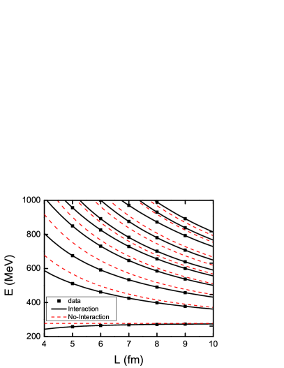
Figure 2: (Color online) The spectrum of $\pi\pi$ states in the $1b-1c$ model. The black curves are calculated by using the finite-volume Hamiltonian approach. The boxes denote discrete points on these curves which are used in the phase extraction shown in Fig. 3.

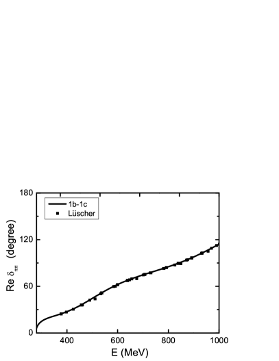
Figure 3: The black curve is generated from directly solving scattering equations Eqs.(6)-(7), and the solid squares are calculated from using the Lüscher’s method by using the spectrum appearing in Fig. 2.

In comparison with realistic lattice calculations, we note that the smooth reproduction of the phase shift would require significant resources in terms of the number of volumes sampled. Such a dense extraction of the phase shift is more easily made possible by studying the spectra in moving frames, such as Ref. Dudek:2012xn ; Rummukainen:1995vs ; Kim:2005gf ; Fu:2011xz ; Leskovec:2012gb ; Gockeler:2012yj . The extension of the Hamiltonian formalism to such boosted systems will be investigated in future work.

With the equivalence with the Lüscher technique demonstrated, we now turn to the extension to multi-channel scattering.

IV one bare state and two-channels

IV.1 Model parameters

To describe $\pi\pi$ scattering above the $K\bar{K}$ threshold, we construct a model with one bare state and two-channels. The formula for such a model can be obtained from Section II by setting $n=1$ for a bare particle $\sigma$ and $\alpha,\beta,\gamma=\pi\pi,K\bar{K}$. Similar to the $1b-1c$ model of section III, the matrix elements of the interactions defined in Eqs.(4) and (5) are parameterized as

$$\langle\sigma|g|\alpha(\vec{k})\rangle = g_{\sigma,\alpha}(k)$$ (28)

$$= \frac{g_{\sigma,\alpha}}{\sqrt{\pi}}\frac{1}{(1+(c_{\alpha}\times k)^{2})},$$

$$\langle\alpha(\vec{k})|v|\beta(\vec{k}^{\prime})\rangle = v_{\alpha,\beta}(k,k^{\prime})$$ (29)

$$= \frac{G_{\alpha,\;\beta}}{m^{2}_{\pi}}\times\frac{1}{(1+(d_{\alpha}\times k)^{2})^{2}}\times\frac{1}{(1+(d_{\beta}\times k^{\prime})^{2})^{2}},$$

with $k$ and $k^{\prime}$ are the three momenta of $\pi$ or $K$ in the center mass system. There are ten parameters: $m_{\sigma}$, $g_{\pi\pi}$, $c_{\pi\pi}$, $g_{K\bar{K}}$, $c_{K\bar{K}}$, $G_{\pi\pi,\;\pi\pi}$, $G_{\pi\pi,\;K\bar{K}}$, $G_{K\bar{K},\;K\bar{K}}$ $d_{\pi\pi}$ and $d_{K\bar{K}}$. By fitting the data of $\pi\pi$ phase shift $\delta$ and inelasticity $\eta$, the model parameters can be determined and are listed in the second column of Table 1. The calculated phase shifts are compared with the data in Figs. 4–6. As in the single channel case, the agreement is sufficiently good for our exploration of the finite volume Hamiltonian method.

Figure 4: The phase shift $\delta_{\pi\pi}$ for $\pi\pi$ scattering from the $1b-2c$ model are compared with the data.

Figure 5: The phase shift $\delta_{K\bar{K}}$ of $K\bar{K}$ scattering calculated in the $1b-2c$ model.

Figure 6: The inelasticity $\eta$ in the $1b-2c$ model compared with the data.

IV.2 Finite-volume Hamiltonian method

To calculate the spectrum for the $1b-2c$ model constructed in the previous subsection, we follow the procedures given in Section III.2 to extend the matrix representation of the Hamiltonian to include the elements associated with the additional $K\bar{K}$ channel for each mesh points of the chosen $N$ momenta $k_{n}=\sqrt{n}\frac{2\pi}{L}$ for $n=0,1,2\cdot\cdot\cdot(N-1)$. This leads to the following $(2N+1)\times(2N+1)$ matrix equations

$$\det([H_{0}]_{2N+1}+[H_{I}]_{2N+1}-E[I]_{2N+1})=0$$ (30)

where $[I]_{2N+1}$ is an $(2N+1)\times(2N+1)$ unit matrix, and

$$[H_{0}]_{2N+1} = \left(\begin{array}[]{cccccccc}m_{0}&0&0&0&0&\cdots\\ 0&2\sqrt{k^{2}_{0}+m^{2}_{\pi}}&0&0&0&\cdots\\ 0&0&2\sqrt{k^{2}_{0}+m^{2}_{K}}&0&0&\cdots\\ 0&0&0&2\sqrt{k^{2}_{1}+m^{2}_{\pi}}&0&\cdots\\ 0&0&0&0&2\sqrt{k^{2}_{1}+m^{2}_{K}}&\cdots\\ \vdots&\vdots&\vdots&\vdots&\vdots&\ddots\end{array}\right)$$ (37)

The $(2N+1)\times(2N+1)$ matrix for the interaction Hamiltonian is

$$[H_{I}]_{2N+1} = \left(\begin{array}[]{cccccccc}0&g^{fin}_{\pi\pi}(k_{0})&g^{fin}_{K\bar{K}}(k_{0})&g^{fin}_{\pi\pi}(k_{1})&g^{fin}_{K\bar{K}}(k_{1})&\cdots\\ g^{fin}_{\pi\pi}(k_{0})&v^{fin}_{\pi\pi,\pi\pi}(k_{0},k_{0})&v^{fin}_{\pi\pi,K\bar{K}}(k_{0},k_{0})&v^{fin}_{\pi\pi,\pi\pi}(k_{0},k_{1})&v^{fin}_{\pi\pi,K\bar{K}}(k_{0},k_{1})&\cdots\\ g^{fin}_{K\bar{K}}(k_{0})&v^{fin}_{K\bar{K},\pi\pi}(k_{0},k_{0})&v^{fin}_{K\bar{K},K\bar{K}}(k_{0},k_{0})&v^{fin}_{K\bar{K},\pi\pi}(k_{0},k_{1})&v^{fin}_{K\bar{K},K\bar{K}}(k_{0},k_{1})&\cdots\\ g^{fin}_{\pi\pi}(k_{1})&v^{fin}_{\pi\pi,\pi\pi}(k_{1},k_{0})&v^{fin}_{\pi\pi,K\bar{K}}(k_{1},k_{0})&v^{fin}_{\pi\pi,\pi\pi}(k_{1},k_{1})&v^{fin}_{\pi\pi,K\bar{K}}(k_{1},k_{1})&\cdots\\ g^{fin}_{K\bar{K}}(k_{1})&v^{fin}_{K\bar{K},\pi\pi}(k_{1},k_{0})&v^{fin}_{K\bar{K},K\bar{K}}(k_{1},k_{0})&v^{fin}_{K\bar{K},\pi\pi}(k_{1},k_{1})&v^{fin}_{K\bar{K},K\bar{K}}(k_{1},k_{1})&\cdots\\ \vdots&\vdots&\vdots&\vdots&\vdots&\ddots\end{array}\right),$$ (44)

with

$$g^{fin}_{\alpha}(k_{n}) = \sqrt{\frac{C_{3}(n)}{4\pi}}\left(\frac{2\pi}{L}\right)^{3/2}g_{\sigma,\alpha}(k_{n}),$$ (45)

$$v^{fin}_{\alpha,\beta}(k_{n_{i}},k_{n_{j}}) = \sqrt{\frac{C_{3}(n_{i})}{4\pi}}\sqrt{\frac{C_{3}(n_{j})}{4\pi}}\left(\frac{2\pi}{L}\right)^{3}v_{\alpha,\beta}(k_{n_{i}},k_{n_{j}}),$$ (46)

where $g_{\sigma,\alpha}(k_{n})$ and $v_{\alpha,\beta}(k_{n_{i}},k_{n_{j}})$ are defined in Eqs. (28) and (29). In this way, we can generate the spectrum from the Hamiltonian in a finite box with a given size $L$ by solving Eq. (30). The computed spectrum is shown as a function of the volume in Fig. 7.

As discussed in the previous section, we are neglecting the physics associated with the multiparticle thresholds (eg. $4\pi$ at $E\sim 560\,{\rm MeV}$). We thereby focus our attention on the issues related to the coupled-channel system, while maintaining a realistic representation of observed scattering in QCD.

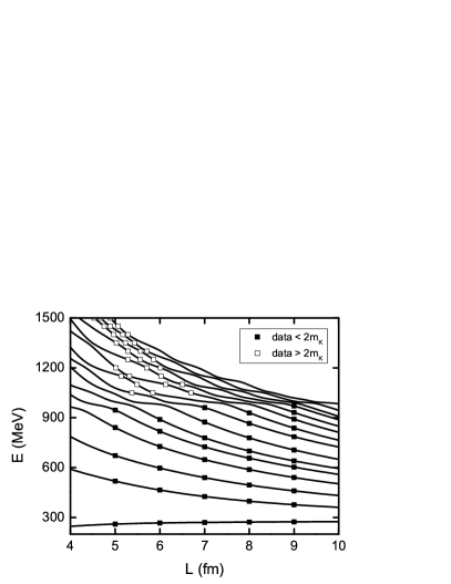
Figure 7: The black curves show the energy spectra generated by using the finite-box Hamiltonian approach within the the $1b-2c$ model. The solid and open squares are selected solutions below and above the inelastic threshold, respectively. These solutions have been inverted through the extended Lüscher formalism to determine the phase shifts and inelasticities, see Fig. 9.

IV.3 Multi-channel spectra

Our first task here is to establish the equivalence of the Hamiltonian spectrum with that of the multi-channel generalisation of Lüscher. The relevant formulae for the coupled-channel system are summarised in Appendix A.2. For the present case, the eigenvalue spectrum (above the inelastic threshold) is defined by the solutions to the following equation

$$\cos\left[\phi(q_{\pi\pi})+\phi(q_{K\bar{K}})-\delta_{\pi\pi}(E)-\delta_{K\bar{K}}(E)\right]$$

$$\quad-\eta(E)\cos\left[\phi(q_{\pi\pi})-\phi(q_{K\bar{K}})-\delta_{\pi\pi}(E)+\delta_{K\bar{K}}(E)\right]=0.$$ (47)

The phase $\phi$ characterises the lattice geometry as defined by Eq. (59). Knowledge of the energy-dependence of the phase shifts and inelasticity allows one to determine the spectrum for a given value of $L$. The eigenvalue equation is solved for $E$, where the dimensionless momenta, $q_{\alpha}=k_{\alpha}L/(2\pi)$, corresponding to the on-shell momentum $k_{\alpha}$ in channel $\alpha$ (see Eq. (58)).

Using the model phase shifts and inelasticities, the Lüscher-style formalism allows one to uniquely determine the finite volume spectrum. For this model, the solutions of Eq. (47) (in the inelastic region) are shown in Fig. 8. The predicted spectra within the two approaches are in excellent agreement — hence confirming that the spectra are determined by the same asymptotic eigenvalue constraint.

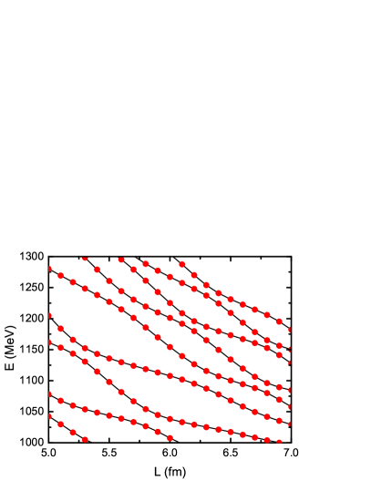
Figure 8: (Color online) The solid dots represent the finite volume spectrum as determined by the extended Lüscher formalism; computed directly from the model phase shifts and inelasticities. These are in excellent agreement with the spectra computed with the Hamiltonian approach, as shown by the continuous curves.

Of relevance to lattice QCD simulations is the desire to obtain $\delta_{\pi\pi}$, $\delta_{K\bar{K}}$ and $\eta$ from the spectra determined in numerical simulations. Using Eq. (66), the isolation of all three scattering parameters at any given $E$ would require eigenstates at this energy for three different box sizes. Such solutions are indicated by the white squares in Fig. 7. Across an ensemble of volumes, the extraction of the resonance parameters from the asymptotic constraints of the Lüscher quantisation alone, can only lead to a “pointwise” determination of the scattering parameters. Such a “pointwise” inversion for the coupled-channel systems was discussed by Guo et al. Guo:2012hv . Here it was demonstrated that by using multiple different total momentum quantisations of the system, there is an increased opportunity to identify near-degenerate eigenstates such that at least three independent qualisations can be used to model-independently extract the scattering parameters. Nevertheless, it is generally true for any finite set of discrete spectra, the pointwise extraction will only have a limited applicability.

For an example of the inversion in the present case, at $E=1200\,{\rm MeV}$, with box sizes $L=5.022,5.708,6.014\,{\rm fm}$, the model spectrum can be inverted through Eq. (66) to determine

$$\delta_{\pi\pi}=256.5^{\circ},\quad\delta_{K\bar{K}}=79.84^{\circ},\quad\eta=0.6980.$$ (48)

We note the relative phase between $\delta_{\pi\pi}$ and $\delta_{K\bar{K}}$ is only determined up to integer multiples of $\pi$ — an ambiguity that has been elaborated on in Ref. Berkowitz:2012xq . Up to the determination of this phase, we note excellent agreement with the underlying model scattering,

$$\delta_{\pi\pi}=256.6^{\circ},\quad\delta_{K\bar{K}}=80.18^{\circ},\quad\eta=0.6965.$$ (49)

The extraction of $\delta_{\pi\pi}$ in this way, for a range of energies, is shown by the white squares in Fig. 9.

To make the most of a finite set of spectrum “data”, Ref. Guo:2012hv have proposed using a $K$-matrix formulation to parameterise the $S$-matrix and thereby the predicted spectrum. In the following Section we explore the use of the Hamiltonian formulation as an alternative parameterisation to fit a finite set of lattice spectra. Both the Hamiltonian and $K$-matrix approaches have been used extensively to extract from scattering observables the resonance parameters associated with the excited hadrons; as reviewed in Ref. Burkert:2004sk for the excited nucleons. It has been well recognised that the comparisons of the results from these two different approaches are fruitful in making progress to establish the hadron spectra; as can be seen in the coupled-channel analysis results presented in Refs. Kamano:2013iva ; Anisovich:2011fc ; Ronchen:2012eg .

We note that the main point of our approach is to relate the spectrum in a finite volume to the asymptotic properties of scattering wavefunctions directly through a procedure of diagonalizing a Hamiltonian; rather than indirectly through the scattering parameters. Our numerical results presented above show that this procedure is equivalent to the Lüscher formulation for the coupled-channel case. Thus our approach is readily applicable to the case with more than two particles, for which the corresponding Lüscher formulation has not yet been developed. This marks the main difference between our work with that of Ref. Guo:2012hv , and similarly related work.

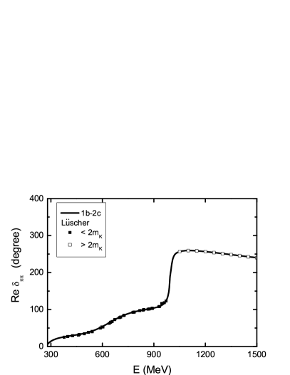
Figure 9: The black curve denotes the model $\pi\pi$ phase shift. The solid and open squares denote the inversion of the solutions shown in Fig. 7 below and above the inelastic thresholds. Below the inelastic threshold, each solution uniquely determines the phase shift. Above the inelastic threshold, the unique solution requires the impractical determination of three identical energy levels at different $L$. In this region, $\delta_{K\bar{K}}$ and $\eta$ (Figs. 5 and 6) are equally-well described by this inversion.

V Applications to LQCD

We investigate the procedure for using the Hamiltonian approach to predict the scattering observables from the spectrum generated from LQCD. We will compare our approach with the approach based on Lüscher’s formula. For this illustrative purpose, it is sufficient to use the $1b-1c$ and $1b-2c$ models described in sections III and IV to generate the spectra which will be referred to as the “LQCD data”. The phase shifts at each energy of these spectra are of course known, as shown as the solid curves in Figs. 1 and 4–6.

Our procedure is to use a Hamiltonian to fit a given choice of the spectrum data by solving the eigenvalue problem defined by Eqs.(15)-(27) for the one-channel case and Eqs.(30)-(46) for the two-channel case. We then use the determined Hamiltonian to calculate the phase shifts by using the scattering equations Eqs.(6)-(7) in infinite space.

To proceed, we need to choose the forms of the interactions in Eqs. (1)–(5) of the phenomenological Hamiltonian. For simplicity, we consider the Hamiltonian which has either one bare state and one-channel or one bare state and two-channels. These Hamiltonians are similar to the $1b-1c$ and $1b-2c$ models constructed in sections III and IV, but they can have a different parametrization of the vertex interaction $g_{\sigma,\alpha}$ and $v_{\alpha,\beta}$. We consider three forms:

• A:

  $$g(k)_{\sigma,\alpha} = \frac{g_{\alpha}}{\sqrt{\pi}}\frac{1}{(1+(c_{\alpha}\times k)^{2})},$$ (50)

  $$v_{\alpha,\beta}(k,k^{\prime}) = \frac{G_{\alpha,\;\beta}}{m^{2}_{\pi}}\times\frac{1}{(1+(d_{\alpha}\times k)^{2})^{2}}\times\frac{1}{(1+(d_{\beta}\times k^{\prime})^{2})^{2}},$$ (51)

• B:

  $$g(k)_{\sigma,\alpha} = \frac{g_{\alpha}}{\sqrt{\pi}}\frac{1}{(1+(c_{\alpha}\times k)^{2})^{2}},$$ (52)

  $$v_{\alpha,\beta}(k,k^{\prime}) = \frac{G_{\alpha,\;\beta}}{m^{2}_{\pi}}\times\frac{1}{(1+(d_{\alpha}\times k)^{2})^{4}}\times\frac{1}{(1+(d_{\beta}\times k^{\prime})^{2})^{4}},$$ (53)

• C:

  $$g(k)_{\sigma,\alpha} = \frac{g_{\alpha}}{\sqrt{\pi}}e^{-(c_{\alpha}\times k)^{2}},$$ (54)

  $$v_{\alpha,\beta}(k,k^{\prime}) = \frac{G_{\alpha,\beta}}{m^{2}_{\pi}}e^{-(d_{\alpha}\times k)^{2}}e^{-(d_{\beta}\times k^{\prime})^{2}},$$ (55)

  Note that the parametrization $A$ is the same as those of models $1b-1c$ and $1b-2c$, as described above.

V.1 Fit for one-channel

We first consider the one-channel case. The spectrum data are generated from model $1b-1c$ constructed in section III. In the left side of Fig. 10, we show 8 data points generated by solving the eigenvalue equation, Eq. (15), for $L=5,6$ fm. For the discussion of this manuscript, the choice of $L$ values is largely irrelevant. The smaller of these volumes has $m_{\pi}L\sim 3.5$, which is just below the reputed value of 4. As such, it is plausible that there are non-negligible corrections associated with the exponentially suppressed finite-volume effects Bedaque:2006yi ; Chen:2012rp ; Albaladejo:2013bra . While we neglect these effects in the present study, they will certainly be of relevance in future precision studies.

To see whether the fit depends sensitively on the form of the Hamiltonian, we assign a very small ($1$ MeV) error for each energy level in the spectrum. We find that these 8 spectrum data points can be fitted by using the parametrization $B$, or $C$, as shown in the left side of Fig.10. The $\pi\pi$ phase shifts calculated from two new Hamiltonians using the scattering equations Eqs. (6)–(7) in infinite space are compared with the data (solid squares) in the right side of Fig. 10. They agree very well in the energy region $E$ $\lesssim$ 0.9 GeV, where the spectrum data are fitted. At higher energies, the calculated phase shifts from $B$ and $C$ deviate from each other and also from the $1b-1c$ model. Note that both the black solid curves ($A$) and data (solid squares) are from the $1b-1c$ model and thus they agree with each other completely.

The results presented above suggest that the finite-box Hamiltonian approach is valid in the energy region where the spectrum data are fitted, since the predicted scattering phase shifts are independent of the form of the Hamiltonian and agree with the phase shifts corresponding the fitted spectrum data. To further examine this, we generate 16 data points up to 1.2 GeV and repeat the fitting process. The generated data are the black squares in the left side of Fig.11. The predicted phase shifts agree with the data in the $E<$ 1.2 GeV region where the spectrum data are fitted. Above 1.2 GeV they deviate from the the $1b-1c$ model, similar to what we observed in Fig.10.

With the results shown in Figs. 10–11 and the Fig. 2 on Lüscher’s method in section III, we conclude that the finite-volume Hamiltonian approach gives a comparable reproduction of the phase shifts as compared to Lüscher’s method. However, for the one-channel case the finite-volume Hamiltonian method has no distinct advantage over Lüscher’s method, since the required LQCD efforts are not so different.

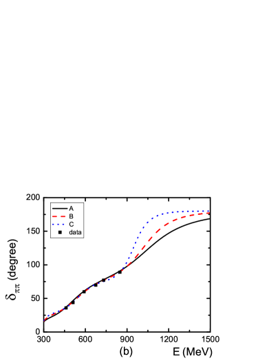
Figure 10: (Color online) (a): the spectrum data generated from $1b-1c$ model. (b): the phase shifts calculated from the one-channels model with parametrization $A$ ($1b-1c$ model) and $B$ and $C$ specified in Eqs.(50)-(55) are compared with the data (from $1b-2c$ model).

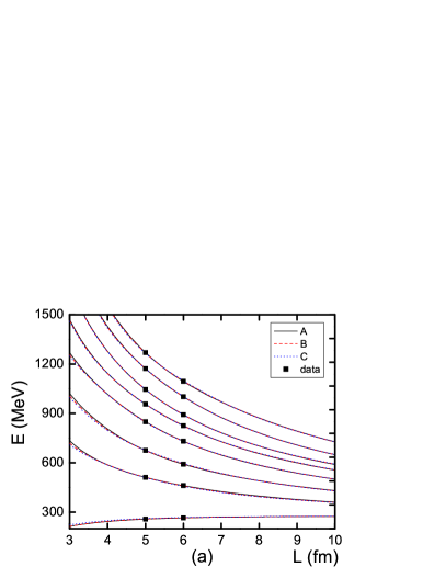
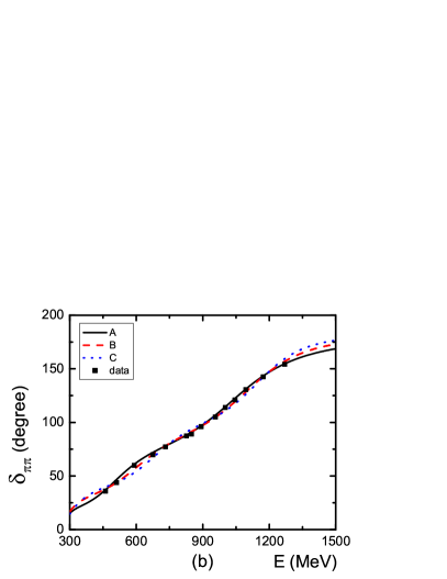
Figure 11: (Color online) (a): the spectrum data generated from $1b-1c$ model. (b): the phase shifts calculated from the one-channels model with the parametrization $A$ ($1b-1c$ model), $B$ and $C$ specified in Eqs.(50)-(55) are compared with the data (from $1b-1c$ model).

V.2 Fit for two-channels

Here we explore the finite-volume Hamiltonian method for the coupled-channels system. We generate 16 and 24 spectrum data points from the $1b-2c$ model constructed in section IV.A by solving eigenvalue problem defined by Eqs.(30)-(46) for $L=$ 5, 6 fm. As shown in the left top panel of Figs. 12 and 13, these spectrum data can be fit by a Hamiltonian with the parametrization $B$ or $C$ of the interaction Hamiltonian specified in Eqs. (52)–(55). As in the one-channel case, we assign a 1 MeV error for each spectrum data point in these fits. We see in Figs. 12–13 that the phase shifts $\delta_{\pi\pi}$ and $\delta_{K\bar{K}}$ and inelasticity $\eta$ calculated from the determined Hamiltonians agree well with data (from model $1b-2c$) in the energy region where the spectrum data are fitted. Similar to the one-channel case, the predicted phase shifts deviate from each other outside the energy range of the fitted spectrum data. We thus conclude that the finite-volume Hamiltonian offers a method to directly extract the scattering parameters from numerical simulation.

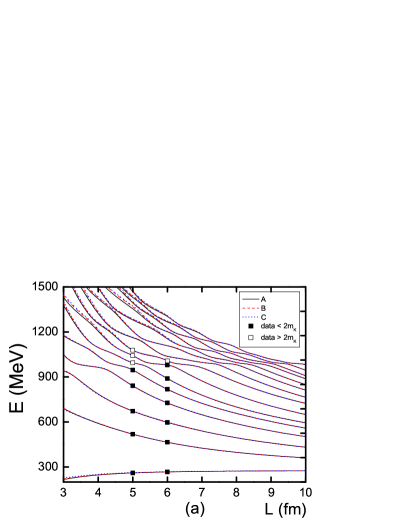
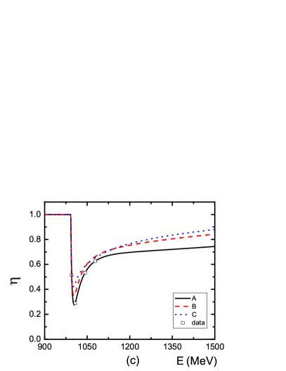
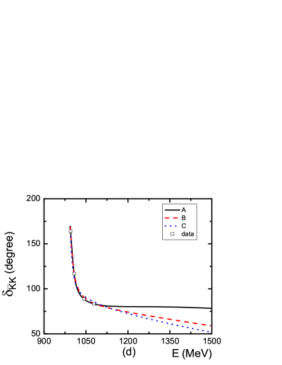
Figure 12: (Color online) (a): the spectrum data generated from $1b-2c$ model. (b-d): the phase shifts and the inelasticity calculated from the two-channels model with the parametrization $A$ ($1b-2c$ model), $B$ and $C$ specified in Eqs.(50)-(55) are compared with the data (from $1b-2c$ model).

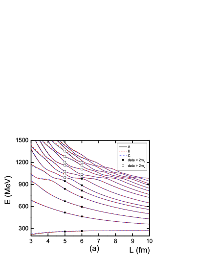
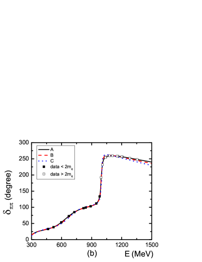
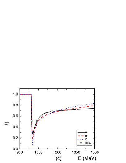
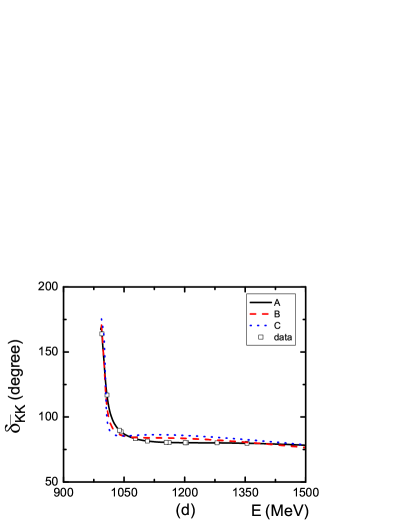
Figure 13: (Color online) (a): the spectrum data generated from $1b-2c$ model. (b-d): the phase shifts and the inelasticity calculated from the one-channels model with the parametrization $A$ ($1b-2c$ model), $B$ and $C$ specified in Eqs.(50)-(55) are compared with the data (from $1b-2c$ model).

Furthermore, the method is largely independent of the form of the Hamiltonian. One should caution that the resulting Hamiltonian can only be reliably used to predict the scattering observables in the energy region where the lattice spectra are fit — as also seen in the single-channel case.

Here we point out an important difference with the approach using the two-channel Lüscher’s formula. As we discussed in section IV, the two-channel Lüscher formula, Eq. (47), needs three spectrum data points at the same energy to calculate two phase shifts and inelasticity. Thus the spectrum data (open squares) in the left top panel of Figs. 12 and 13 are not sufficient to apply the Lüscher’s method. One thus requires many more calculations to get a spectrum like the open squares shown in Fig.9 in section IV. For a given $E$, we need to get results for three values of $L$, which can be chosen only after some searches, since we don’t know the spectrum for each $L$ before the calculation is finished. Alternatively, the finite-box Hamiltonian method offers a method to interpolate the lattice spectra with a minimal set of volumes. Further, the quality of the extraction will naturally improve more simulation results.

Finally, regarding the relative phase ambiguity mentioned above Berkowitz:2012xq , in the present context of the Hamiltonian formulation, the finite volume spectra cannot fix the relative sign of the resonance coupling to different channels, Eq. (28), nor the sign of the off-diagonal terms in the direct interaction, Eq. (29). Again, these signs only act to constrain the relative phase between $\delta_{\pi\pi}$ and $\delta_{K\bar{K}}$ but do not influence the energy dependence or the isolation of the resonance pole position.

VI Spectra from $\pi\pi$ data

As a final investigation for the present study, we comment on the possibility of lattice QCD providing the necessary knowledge to improve on phenomenological scattering parameterisations.

Within the Hamiltonian formulation given in section II, the $\pi\pi$ scattering phase shifts $\delta_{\pi\pi}$ and inelasticity $\eta$ up to 2 GeV have been fit Kamano:2011ih using a model which has two bare states and includes the $\pi\pi$ and $K\bar{K}$ channels. Its interaction Hamiltonian only has the vertex interaction $g$ defined in Eq. (4). This model (which we will refer to as NKLS) also reproduces well the resonance pole positions listed by the Particle Data Group PDG . We explore a further two models, $B$ and $C$, which further incorporate the two-body interaction $v$ defined in Eq. (5) with the form Eq. (51). These two solutions give equally good fits to the data of $\delta_{\pi\pi}$ and inelasticity $\eta$, and the resonance pole positions. The three models for both S-wave and P-wave scattering are shown in Figs. 14 and 15, with model parameters listed in Table 2. Note that the parametrization of the matrix elements of the interactions of NKLS model are the same as Model $A$ specified in Eq.(50) and (51) except that the parametrization for the p-wave vertex interaction in the $J^{IP}=1^{1-}$ partial wave is

$$\langle k|g_{\sigma,i}\rangle = g_{\sigma,i}(k)$$ (56)

$$= \frac{g_{i}}{\sqrt{m_{\pi}}}\left(\frac{1}{(1+(c_{\pi\pi}\times k)^{2})}\right)^{\frac{3}{2}}\frac{k}{m_{\pi}},$$

As there are no data to constrain the $K\bar{K}$ scattering phase shifts, this observable displays the largest variation among the model solutions — see the right panel of Figs. 14 and 15. We can now explore the sensitivity to this variation in the predicted finite volume spectra. These predicted spectra are show in Fig. 16. While the spectra are in broad agreement between the models, there are noticeable differences among the volumes considered. In particular, on the $4\,{\rm fm}$ box some energy levels see a variation of up to $50\,{\rm MeV}$ between the different model solutions. In principle, lattice QCD spectra of this order of precision could act to further constrain this phenomenological model. One should of course caution that, in principle, there could be further inelastic channels appearing in the lattice calculation — such as 4 pions.

Table 2: The parameters of the Hamiltonians from fitting the phase shift data of $\pi\pi$ scattering in s-wave $J^{IP}=0^{0+}$ and p-wave $J^{IP}=1^{1-}$ partial waves.

	S-wave			P-wave
Parameter	NKLS	B	C	NKLS	B	C
$m_{\sigma_{1}}$(MeV)	$1220.0$	$1094.28$	$1300.00$	$891.54$	$900.000$	$999.950$
$g_{\sigma_{1}\pi\pi}$	$-0.63474$	$-0.97085$	$-0.51274$	$-0.20583$	$-0.15561$	$-0.11669$
$c_{\sigma_{1}\pi\pi}$(fm)	$0.44658$	$0.50923$	$0.33070$	$0.49998$	$0.41213$	$0.31296$
$g_{\sigma_{1}K\bar{K}}$	$0.00605$	$1.64234$	$0.07659$	$0.10607$	$0.01010$	$0.00128$
$c_{\sigma_{1}K\bar{K}}$(fm)	$0.10012$	$2.29463$	$0.17073$	$0.42241$	$0.17333$	$0.04512$
$m_{\sigma_{2}}$(MeV)	$2400.0$	$1907.63$	$2318.94$	$1840.0$	$1657.66$	$1903.56$
$g_{\sigma_{2}\pi\pi}$	$0.49518$	$0.49178$	$1.43296$	$0.01453$	$0.01852$	$0.00517$
$c_{\sigma_{2}\pi\pi}$(fm)	$0.20645$	$0.31107$	$0.35299$	$0.10000$	$0.15068$	$0.06607$
$g_{\sigma_{2}K\bar{K}}$	$-1.17880$	$-1.53414$	$-2.50030$	$0.16674$	$2.42851$	$0.10514$
$c_{\sigma_{2}K\bar{K}}$(fm)	$0.50000$	$1.06150$	$0.79294$	$0.49993$	$1.71022$	$0.30817$
$G_{\pi\pi,\;\pi\pi}$	$-$	$0.10000$	$0.10000$	$-$	$-0.01718$	$0.00024$
$G_{\pi\pi,\;K\bar{K}}$	$-$	$-0.00045$	$-0.07138$	$-$	$-0.11589$	$-0.04689$
$G_{K\bar{K},\;K\bar{K}}$	$-$	$-0.00016$	$0.09992$	$-$	$0.34790$	$0.02819$
$d_{\pi\pi}$(fm)	$-$	$0.27088$	$0.18337$	$-$	$0.42441$	$0.26895$
$d_{K\bar{K}}$(fm)	$-$	$0.00551$	$0.18402$	$-$	$0.41520$	$0.12503$
$\chi^{2}$	$305$	$205$	$215$	$189$	$119$	$119$
Pole(GeV)	$0.43-0.27i$	$0.43-0.32i$	$0.43-0.26i$	$0.77-0.081i$	$0.77-0.075i$	$0.77-0.076i$
	$1.0-0.010i$	$1.0-0.014i$	$1.0-0.008i$	$1.61-0.11i$	$1.63-0.075i$	$1.65-0.083i$
	$1.35-0.17i$	$1.51-0.22i$	$1.52-0.20i$	$-$	$-$	$-$

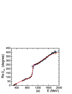
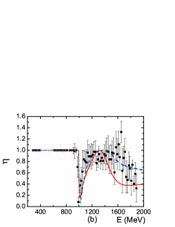
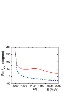
Figure 14: (Color online) The phase shifts $\delta_{\pi\pi}$ and $\delta_{K\bar{K}}$, and inelasticity $\eta$ of s-wave $\pi\pi$ scattering in the $J^{IP}=1^{0+}$ partial wave. The solid squares are the experiment data. The red solid, blue dashed and green dotted lines are from the NKLS model, Model B, and Model C, respectively.

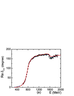
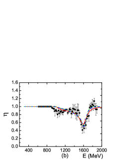
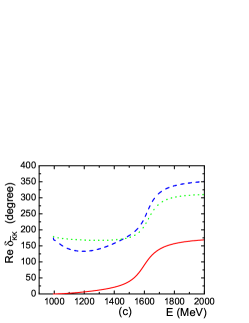
Figure 15: (Color online) The phase shifts $\delta_{\pi\pi}$ and $\delta_{K\bar{K}}$, and inelasticity $\eta$ of p-wave$\pi\pi$ scattering in the $J^{IP}=1^{1-}$ partial wave. The solid squares are the experiment data. The red solid, blue dashed and green dotted lines are from the NKLS model, Model B, and Model C, respectively.

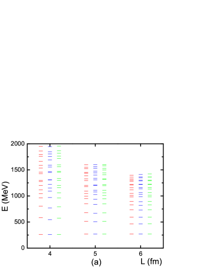
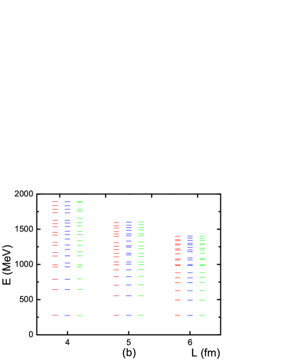
Figure 16: (Color online) Spectra for $J^{IP}=0^{0+}$(left) and $J^{IP}=1^{1-}$(right) partial waves from Models NKLS, Model B and Model C. The spectra have been displaced for clarity.

VII Summary

We have investigated the finite-volume Hamiltonian method developed in Ref. Hall:2013qba within several models for $\pi\pi$ scattering. We have demonstrated the equivalence of the finite volume spectra with the Lüscher formalism for both a single channel and also the corresponding generalisation to a coupled-channel system.

We then investigated the practical inversion problem for lattice QCD, with the aim to determine the physical scattering parameters from the finite-volume spectra. The finite-volume Hamiltonian framework offers a robust framework for the parameterisation of hadronic interactions to fit lattice spectra. Future work will aim to address outstanding issues, as addressed throughout the manuscript, including: the role of angular momentum mixing, exponentially suppressed corrections and multi-particle inelasticities. The generalisation to moving frames will also act to improve the determination of scattering parameters, with little additional computational costs.

Based on phenomenological fits to experimental $\pi\pi$ scattering, we have presented the predicted spectra that one could anticipate seeing in lattice simulations at the physical pion mass. Here we have demonstrated that sufficient precision from lattice QCD simulations would offer the potential to improve the knowledge of these phenomenological models. This is particularly significant for channels that are not directly observable in experiment.

Our investigations are based on a rather phenomenological form of the Hamiltonian. Thus the constructed Hamiltonian from fitting lattice QCD spectrum can not be used reliably to predict scattering observables beyond the energy region where the spectra are fit. One potential improvement in this general framework would be to consider more realistic forms of the Hamiltonian, such as those derived from chiral Lagrangians. This would largely act to improve the near-threshold behaviour of the interactions, however is beyond the scope of the present work.

VIII acknowledgment

We wish to thank Raúl Briceño for helpful correspondence. This work is supported by the U.S. Department of Energy, Office of Nuclear Physics Division, under Contract No. DE- AC02-06CH11357. This research used resources of the National Energy Research Scientific Computing Center, which is supported by the Office of Science of the U.S. Department of Energy under Contract No. DE-AC02-05CH11231, and resources provided on ”Fusion”, 320-node computing cluster operated by the Laboratory Computing Resource Center at Argonne National Laboratory. This work was also supported by the University of Adelaide and the Australian Research Council through the ARC Centre of Excellence for Particle Physics at the Terascale and grants FL0992247 (AWT), DP140103067, FT120100821 (RDY).

Appendix A Lüscher summary

A.1 Single channel

For comparison with Lüscher’s method, we summarise the formulae relevant to a purely s-wave interaction, as considered in this manuscript. It relates each energy eigenvalues $E$ of the finite box with size $L$ to the scattering phase shift $\delta$ at energy $E$ by the following equations:

$$\delta(k) = -\phi(q)+n\pi$$ (57)

with the on-shell momenta given by

$$k=\sqrt{E^{2}/4-m^{2}_{\pi}},$$ (58)

and the geometric phase $\phi$ defined by

$$\tan\phi(q)=-\frac{q\pi^{3/2}}{\mathscr{Z}_{00}(1;q^{2})}\,,$$ (59)

expressed in terms of the lattice momenta

$$q=\frac{kL}{2\pi}.$$ (60)

The generalized zeta function is defined by

$$\mathscr{Z}_{00}(1;q^{2})=\frac{1}{\sqrt{4\pi}}\sum_{\vec{n}\in\mathbb{Z}^{3}}(\vec{n}^{2}-q^{2})^{-1}\,,$$ (61)

defined with an appropriate regularisation of the divergent sum (see eg. Luscher:1990ux for discussion). Numerically, a convenient representation for the evaluation of the regularised form is given by

$$\mathscr{Z}_{00}(1;q^{2}) = \frac{1}{\sqrt{4\pi}}\left(-\frac{1}{q^{2}}-8.91363292+16.53231596q^{2}+\sum_{\vec{n}\in\mathbb{Z}^{3},\vec{n}\neq 0}\frac{q^{4}}{\vec{n}^{4}(\vec{n}^{2}-q^{2})}\right).$$ (62)

A.2 Coupled channel

At energies above the $K\bar{K}$ threshold, we need Lüscher’s method for two open channels, as developed in Ref.He:2005ey . For the considered $\pi\pi$ and $K\bar{K}$ channels, the $S$-matrix is defined by

$$S = \left(\begin{array}[]{cc}\eta e^{2i\delta_{\pi\pi}}&i\sqrt{1-\eta^{2}}e^{i(\delta_{\pi\pi}+\delta_{K\bar{K}})}\\ i\sqrt{1-\eta^{2}}e^{i(\delta_{\pi\pi}+\delta_{K\bar{K}})}&\eta e^{2i\delta_{K\bar{K}}}\end{array}\right),$$ (65)

where the phase shifts $\delta_{\pi\pi}$ and $\delta_{K\bar{K}}$ and inelasticity $\eta$ at each $E$ are related to the box size $L$ by the following relation

$$\cos\left[\phi(q_{\pi\pi})+\phi(q_{K\bar{K}})-\delta_{\pi\pi}(E)-\delta_{K\bar{K}}(E)\right]$$

$$\quad-\eta(E)\cos\left[\phi(q_{\pi\pi})-\phi(q_{K\bar{K}})-\delta_{\pi\pi}(E)+\delta_{K\bar{K}}(E)\right]=0.$$ (66)

where $\phi(q_{\alpha})$ is defined as Eq. (59), and

$$q_{\alpha} = \frac{k_{\alpha}(E)L}{2\pi}.$$ (67)

Appendix B Relationship between the Hamiltonian and Lüscher quantisations

The Lüscher formalism has established that the finite volume spectrum of multi-particle states is determined by an eigenvalue equation involving just the $S$-matrix of the corresponding theory — up to corrections which are exponentially suppressed in $mL$ for large volumes. This has been derived on the basis of the underlying fields satisfy the periodicity of the lattice and that the interactions are finite-range in nature, limited by a mass scale $m$ (typically the lightest particle degree of freedom present in the system). The Hamiltonian formulation presented here, and previously in Ref. Hall:2013qba , has an interaction which is finite ranged and the fields themselves are quantised to satisfy the lattice periodicity. Therefore, in terms of the quantisation condition on the spectra, the Hamiltonian no more than an explicit realisation of the general conditions considered by Lüscher.

In the Sec. III.3 and  IV.3, we have numerically demonstrated the correspondence between the Hamiltonian and Lüscher spectra. In this appendix, for the case of a simple idealised system we provide an analytic derivation of the connection between the Lüscher and Hamiltonian formalisms.

B.1 Hamiltonian quantisation

From the Eqs. (20,25,26), the Hamiltonian matrix for the single-channel case with $v=0$ is given by:

$$[H]_{N+1} = \left(\begin{array}[]{cccccccc}m_{\sigma}&g^{fin}_{\pi\pi}(k_{0})&g^{fin}_{\pi\pi}(k_{1})&\cdots\\ g^{fin}_{\pi\pi}(k_{0})&2\sqrt{k^{2}_{0}+m^{2}_{\pi}}&0&\cdots\\ g^{fin}_{\pi\pi}(k_{1})&0&2\sqrt{k^{2}_{1}+m^{2}_{\pi}}&\cdots\\ \vdots&\vdots&\vdots&\ddots\end{array}\right).$$ (72)

The eigenvalue $E_{i}$ of above matrix is satisfied following equation:

$$E_{i}-m_{\sigma} = \left(\frac{2\pi}{L}\right)^{3}\frac{1}{4\pi}\sum_{\vec{k}_{n}=\frac{2\pi}{L}\vec{n},\,\vec{n}\in\mathbb{Z}^{3}}\frac{g^{2}_{\sigma,\pi\pi}(k_{n})}{E_{i}-2E_{\pi}(k_{n})}.$$ (73)

This can be rearranged to the form

$$E_{i}-m_{\sigma}=\left(\frac{2\pi}{L}\right)^{3}\frac{1}{4\pi}\sum_{\vec{k}_{n}=\frac{2\pi}{L}\vec{n},\,\vec{n}\in\mathbb{Z}^{3}}\left[\frac{E_{i}g^{2}_{\sigma,\pi\pi}(k_{n})}{2(k_{i}^{2}-k_{n}^{2})}-\frac{g^{2}_{\sigma,\pi\pi}(k_{n})}{E_{i}+2E_{\pi}(k_{n})}\right],$$ (74)

with $k_{i}$ implicitly defined by $E_{i}=2\sqrt{m_{\pi}^{2}+k_{i}^{2}}$. To highlight the comparison with the Lüscher eigenvalue equation, we further isolate the pole term,

$$E_{i}-m_{\sigma}=\left(\frac{2\pi}{L}\right)^{3}\frac{1}{4\pi}\sum_{\vec{k}_{n}=\frac{2\pi}{L}\vec{n},\,\vec{n}\in\mathbb{Z}^{3}}\left[\frac{E_{i}g^{2}_{\sigma,\pi\pi}(k_{i})}{2(k_{i}^{2}-\vec{k}_{n}^{2})}+\frac{E_{i}\left(g^{2}_{\sigma,\pi\pi}(k_{n})-g^{2}_{\sigma,\pi\pi}(k_{i})\right)}{2(k_{i}^{2}-\vec{k}_{n}^{2})}-\frac{g^{2}_{\sigma,\pi\pi}(k_{n})}{E_{i}+2E_{\pi}(k_{n})}\right].$$ (75)

The last two terms of the RHS have no singularities, and hence this discrete sum can be approximated by the continuum intergal (up to corrections of the order of $e^{-m_{\pi}L}$). Moving the principal value parts of the sum to the LHS

$$E_{i}-m_{\sigma}-\Sigma_{L}^{\rm PV}(E_{i})=\frac{E_{i}g^{2}_{\sigma,\pi\pi}(k_{i})}{8\pi}\left(\frac{2\pi}{L}\right)^{3}\sum_{\vec{k}_{n}=\frac{2\pi}{L}\vec{n},\,\vec{n}\in\mathbb{Z}^{3}}\frac{1}{(k_{i}^{2}-\vec{k}_{n}^{2})},$$ (76)

where $\Sigma_{L}^{\rm PV}$ denotes the finite-volume implementation of the real part of the self energy. We do note that in performing this separation we have introduced ultraviolet divergences to both sides of the equation, these of course exactly cancel each other and have no significance in determining the infrared properties associated with the finite volume quantisation.

B.2 Lüscher quantisation

With the conventional parameterisation of the S matrix, $S=\exp(2i\delta)$, and our definition of the T=matix given by Eqs. (10-12), the phase shift $\delta$ can be directly evaluted from the equation

$$k_{on}\cot\delta(E) = -\frac{4}{\pi E}t^{-1}(E)+ik_{on},$$ (77)

where $k_{on}$ is the on-shell momentum of single pion for total center mass energy E.

With $H_{I}=g$, the $t$ of $\pi\pi$ channel is:

$$t(E) =\frac{g^{2}_{\sigma,\pi\pi}}{E-m_{\sigma}-\Sigma(E)},$$ (78)

$$\Sigma(E) =\int k^{2}dk\frac{g^{2}_{\sigma,\pi\pi}(k)}{E-2E_{\pi}(k)+i\varepsilon},$$ (79)

and hence the phase shift is given by:

$$k_{on}\cot\delta(E) = \frac{-4}{\pi E}\frac{1}{g^{2}_{\sigma,\pi\pi}(k_{on})}\left(E-m_{\sigma}-\Sigma^{\rm PV}(E)]\right).$$ (80)

Neglecting the influence of the partial wave mixing, and any exponentially suppressed corrections, the eigenvalue equation of the Lüscher formalism can be expressed as

$$k_{on}\cot\delta(k_{on})=\frac{2}{\sqrt{\pi}L}\mathscr{Z}_{00}(1;q_{on}^{2}),$$ (81)

with $q_{on}=k_{on}L/(2\pi)$. Equating Eq. (81) with the exact model phase shift of Eq. (80) with some straightforward manipulation yields:

$$E-m_{\sigma}-\Sigma^{\rm PV}(E)=\frac{E_{i}g^{2}_{\sigma,\pi\pi}(k_{i})}{8\pi}\left(\frac{2\pi}{L}\right)^{3}\sum_{\vec{k}_{n}=\frac{2\pi}{L}\vec{n},\,\vec{n}\in\mathbb{Z}^{3}}\frac{1}{(k_{i}^{2}-\vec{k}^{2})}.$$ (82)

This we recognise as the same eigenvalue equation described by the Hamiltonian formulation in Eq. (76), up to the difference $\Sigma^{\rm PV}-\Sigma_{L}^{\rm PV}$ — which is known to be exponentially suppressed.

References

- (1) J. J. Dudek, R. G. Edwards, B. Joo, M. J. Peardon, D. G. Richards and C. E. Thomas, Phys. Rev. D 83, 111502 (2011)
- (2) R. G. Edwards, J. J. Dudek, D. G. Richards and S. J. Wallace, Phys. Rev. D 84, 074508 (2011)
- (3) B. J. Menadue, W. Kamleh, D. B. Leinweber and M. S. Mahbub, Phys. Rev. Lett. 108, 112001 (2012)
- (4) M. S. Mahbub et al. [CSSM Lattice Collaboration], Phys. Rev. D 87, 011501 (2013)
- (5) J. J. Dudek, R. G. Edwards and C. E. Thomas, Phys. Rev. D 87, no. 3, 034505 (2013)
- (6) M. Lüscher, Commun. Math. Phys. 105, 153 (1986).
- (7) M. Lüscher, Nucl. Phys. B 354, 531 (1991).
- (8) J. J. Dudek, R. G. Edwards and C. E. Thomas, Phys. Rev. D 86, 034031 (2012)
- (9) M. Doring, U. G. Meißner, E. Oset and A. Rusetsky, Eur. Phys. J. A 48, 114 (2012)
- (10) M. Doring and U. G. Meißner, JHEP 1201, 009 (2012)
- (11) R. A. Briceno, Z. Davoudi, T. Luu and M. J. Savage, Phys. Rev. D 88, 114507 (2013)
- (12) S. He, X. Feng and C. Liu, JHEP 0507, 011 (2005)
- (13) M. Lage, U. -G. Meißner and A. Rusetsky, Phys. Lett. B 681, 439 (2009)
- (14) V. Bernard, M. Lage, U. -G. Meißner and A. Rusetsky, JHEP 1101, 019 (2011)
- (15) A. Martinez Torres, L. R. Dai, C. Koren, D. Jido and E. Oset, Phys. Rev. D 85, 014027 (2012)
- (16) M. T. Hansen and S. R. Sharpe, Phys. Rev. D 86, 016007 (2012)
- (17) R. A. Briceno and Z. Davoudi, Phys. Rev. D. 88, 094507 (2013)
- (18) N. Li and C. Liu, Phys. Rev. D 87, 014502 (2013)
- (19) P. Guo, J. Dudek, R. Edwards and A. P. Szczepaniak, Phys. Rev. D 88, 014501 (2013)
- (20) J. M. M. Hall, A. C.-P. Hsu, D. B. Leinweber, A. W. Thomas and R. D. Young, Phys. Rev. D 87, 094510 (2013)
- (21) S. Theberge, A. W. Thomas and G. A. Miller, Phys. Rev. D 22, 2838 (1980) [Erratum-ibid. D 23, 2106 (1981)].
- (22) A. W. Thomas, Adv. Nucl. Phys. 13, 1 (1984).
- (23) A. Matsuyama, T. Sato and T. -S. H. Lee, Phys. Rept. 439, 193 (2007)
- (24) H. Kamano, S. X. Nakamura, T. -S. H. Lee and T. Sato, Phys. Rev. C 88, 035209 (2013)
- (25) H. Kamano, S. X. Nakamura, T. S. H. Lee and T. Sato, Phys. Rev. D 84, 114019 (2011)
- (26) K. Polejaeva and A. Rusetsky, Eur. Phys. J. A 48, 67 (2012)
- (27) L. Roca and E. Oset, Phys. Rev. D 85, 054507 (2012)
- (28) S. Kreuzer and H. W. Grießhammer, Eur. Phys. J. A 48, 93 (2012)
- (29) R. A. Briceno and Z. Davoudi, Phys. Rev. D 87, 094507 (2013)
- (30) M. T. Hansen and S. R. Sharpe, arXiv:1311.4848 [hep-lat].
- (31) P. Guo, arXiv:1303.3349 [hep-lat].
- (32) K. Rummukainen and S. A. Gottlieb, Nucl. Phys. B 450, 397 (1995)
- (33) C. h. Kim, C. T. Sachrajda and S. R. Sharpe, Nucl. Phys. B 727, 218 (2005)
- (34) Z. Fu, Phys. Rev. D 85, 014506 (2012)
- (35) L. Leskovec and S. Prelovsek, Phys. Rev. D 85, 114507 (2012)
- (36) M. Gockeler, R. Horsley, M. Lage, U. -G. Meißner, P. E. L. Rakow, A. Rusetsky, G. Schierholz and J. M. Zanotti, Phys. Rev. D 86, 094513 (2012)
- (37) E. Berkowitz, T. D. Cohen and P. Jefferson, arXiv:1211.2261 [hep-lat].
- (38) V. D. Burkert and T. S. H. Lee, Int. J. Mod. Phys. E 13, 1035 (2004)
- (39) A. V. Anisovich, R. Beck, E. Klempt, V. A. Nikonov, A. V. Sarantsev and U. Thoma, Eur. Phys. J. A 48, 15 (2012)
- (40) D. Ronchen, M. Doring, F. Huang, H. Haberzettl, J. Haidenbauer, C. Hanhart, S. Krewald and U. -G. Meißner et al., Eur. Phys. J. A 49, 44 (2013)
- (41) P. F. Bedaque, I. Sato and A. Walker-Loud, Phys. Rev. D 73, 074501 (2006)
- (42) H. -X. Chen and E. Oset, Phys. Rev. D 87, 016014 (2013)
- (43) M. Albaladejo, G. Rios, J. A. Oller and L. Roca, arXiv:1307.5169 [hep-lat].
- (44) J. Beringer et al. [Particle Data Group Collaboration], Phys. Rev. D 86, 010001 (2012).