On the distribution of stellar remnants around massive black holes: slow mass segregation, star cluster inspirals and correlated orbits

Abstract

We use $N$-body simulations as well as analytical techniques to study the long term dynamical evolution of stellar black holes (BHs) at the Galactic center (GC) and to put constraints on their number and mass distribution. Starting from models that have not yet achieved a state of collisional equilibrium, we find that time scales associated with cusp regrowth can be longer than the Hubble time. Our results cast doubts on standard models that postulate high densities of BHs near the GC and motivate studies that start from initial conditions which correspond to well-defined physical models. For the first time, we consider the distribution of BHs in a dissipationless model for the formation of the Milky Way nuclear cluster (NC), in which massive stellar clusters merge to form a compact nucleus. We simulate the consecutive merger of $\sim 10$ clusters containing an inner dense sub-cluster of BHs. After the formed NC is evolved for $\sim 5$ Gyr, the BHs do form a steep central cusp, while the stellar distribution maintains properties that resemble those of the GC NC. Finally, we investigate the effect of BH perturbations on the motion of the GC S-stars, as a means of constraining the number of the perturbers. We find that reproducing the quasi-thermal character of the S-star orbital eccentricities requires $\;\hbox to0.0pt{\lower 2.5pt\hbox{$\sim$}\hss}\raise 1.5pt\hbox{$>$}\;1000$ BHs within $0.1~{}$pc of Sgr A*. A dissipationless formation scenario for the GC NC is consistent with this lower limit and therefore could reconcile the need for high central densities of BHs (to explain the S-stars orbits), with the “missing-cusp” problem of the GC giant star population.

1. introduction

Massive nuclear clusters (NCs) are observed at the center of many galaxies, over the whole Hubble sequence. The frequency of nucleation among galaxies less luminous than $\sim 10^{10.5}~{}L_{\odot}$ is close to $90~{}\%$ as determined by ACS HST observations of galaxies in the Virgo and Fornax galaxy clusters (Carollo et al., 1998; Böker et al., 2002; Côté et al., 2006; Turner et al., 2012). The study of NCs is of great interest for our understanding of galaxy formation and evolution as indicated by the fact that a number of fairly tight correlations are observed between their masses and global properties of their host galaxies such as velocity dispersion and bulge mass (Ferrarese et al., 2006; Wehner & Harris, 2006; Graham & Spitler, 2009; Scott & Graham, 2012; Leigh et al., 2012). Intriguingly, similar scaling relations are obeyed by massive black holes (MBHs) which are predominantly found in massive galaxies that, however, show little evidence of nucleation (e.g., Graham & Spitler, 2009; Neumayer & Walcher, 2012). The existence of such correlations might indicate a direct link among large galactic spacial scales and the much smaller scale of the nuclear environment, and suggests that NCs contain information about the processes that have shaped the central regions of their host galaxies.

How NC formation takes place at the center of galaxies is still largely debated (e.g., Hartmann et al., 2011; Gnedin et al., 2013; Carlberg & Hartwick, 2014; Mastrobuono-Battisti & Perets, 2014). Relatively recent work has shown that “dissipationless” models can reproduce without obvious difficulties the observed properties (Turner et al., 2012) and scaling relations (Antonini, 2013) of NCs. In these models a NC forms through the inspiral of massive stellar clusters into the center due to dynamical friction where they merge to form a compact nucleus (e.g., Tremaine et al., 1975; Capuzzo-Dolcetta & Miocchi, 2008; Capuzzo-Dolcetta, 1993). Alternatively, NCs could have formed locally as a result of radial gas inflow into the galactic center accompanied by efficient dissipative processes (Schinnerer et al., 2008; Milosavljević, 2004). Naturally, dissipative and dissipationless processes are not exclusive and both could be important for the formation and evolution of NCs (Hartmann et al., 2011; Antonini et al., 2012; De Lorenzi et al., 2013).

The Milky Way NC, being only $8~{}$kpc away, is currently the only NC that can be resolved in individual stars and for which a kinematical structure and density profile can be reliably determined (Genzel et al., 2010). This offers the unique possibility to resolve the stellar population, to study the composition and dynamics close to a MBH and put constrains on different NC formation scenarios. The Milky Way NC has an estimated mass of $\sim 10^{7}M_{\odot}$ (Launhardt et al., 2002; Schödel et al., 2009), and it hosts a massive black hole of $\sim 4\times 10^{6}M_{\odot}$ (Genzel et al., 2003; Ghez et al., 2008; Gillessen, 2009) whose gravitational potential dominates over the stellar cusp potential out to a radius of roughly $3$pc - the MBH radius of influence. A handful of other galaxies are also known to contain both a NC and a MBH, which typically have comparable masses (Seth et al., 2008). Population synthesis models suggest that roughly $80\%$ of the stellar mass in the inner parsec of the Milky Way is in ($>5~{}$Gyr) old stars (Pfuhl et al., 2011) although the light is dominated by the young stars. This appears to be typically the case also in most NCs observed in external galaxies (Rossa et al., 2006).

Over the last decades observations of the Galactic NC have led to a number of puzzling discoveries. These include: the presence of a young population of stars (the S-stars) near Sgr A* in an environment extremely hostile to star formation (paradox of youth, Morris, 1993; Schödel et al., 2002); and a significant paucity of red giant stars in the inner half a parsec (conundrum of old age, Merritt, 2010). Number counts of the giant stars at the Galactic center (GC) show that their visible distribution is in fact quite inconsistent with the distribution of stars expected for a dynamically relaxed population near a dominating Keplerian potential (Buchholz et al., 2009; Do et al., 2009; Bartko et al., 2010): instead of a steeply rising Bahcall & Wolf (1976) cusp, there is a $\sim 0.5$ pc core. The lack of a Bahcall-Wolf cusp in the giant distribution casts doubts on dynamical relaxed, quasi-steady-state models of the GC which postulate a high central density of stars and stellar black holes (BHs). In these models the central distribution of stars and BHs is determined by just a handful of parameters: the MBH mass; the total density outside the relaxed region; the slope of the initial mass function (IMF, Merritt, 2013). Given the unrelaxed form of the density profile of stars, making predictions about the distribution of the stellar remnants becomes a much more challenging, time-dependent, problem susceptible to the initial conditions and to the (yet largely unconstrained) formation process of the NC (Antonini & Merritt, 2012).

Understanding the distribution of the “stellar remnants” in systems similar to the Milky Way’s NC is crucial in many respects. Examples include randomization of the S-star orbits via gravitational encounters (Perets et al., 2009), warping of the young stellar disk (Kocsis & Tremaine, 2011), and formation of X-ray binaries (Muno et al., 2005). Stellar nuclei similar to that of the Milky Way are also the location of astrophysical processes that are potential gravitational wave (GW) sources both for ground and space based laser interferometers. These include the merger of compact object binaries near MBHs (Antonini & Perets, 2012), and the capture of BHs by MBHs, called “extreme mass-ratio inspirals” (EMRIs Amaro-Seoane et al., 2012). The efficiency of these dynamical processes and rate estimates for GW sources are very sensitive to the number of BHs near the center. Therefore, a fundamental question is whether given a prediction for the initial distribution of stars and BHs, the system is old enough that the heavy remnants had time to relax and segregate to the center of the Galaxy.

Motivated by the above arguments, we consider the long-term evolution of BH populations at the center of galaxies, starting from different assumptions regarding their initial distribution. Since the stellar BHs at the GC are not directly detected, time-dependent numerical calculations, like the ones presented below, are crucial for understanding and making predictions about the distribution of stellar remnants at the center of galaxies.

In Section 2 we explore the evolution of models in which stars and BHs follow initially the same spatial distribution which is far from being in collisional equilibrium. Contrary to some previous claims (Preto & Amaro-Seoane, 2010), we find that in these models the time to regrow a cusp in both the BH and the star distribution is longer than the age of the Galaxy. For realistic number fractions of BHs, our simulations demonstrate that over the age of the Galaxy the presence of a heavy component has little effect on the evolution of the stellar component.

In Sections 3, 4 and  5 we discuss the evolution of BHs in a globular cluster merger model for NCs. We present the results of direct $N$-body simulations of the merger of globular clusters containing two mass populations: stars and BHs. These systems were in an initial state of mass segregation with the BH population concentrated toward the cluster core. Each cluster was placed on a circular orbit with galactocentric radius of $20~{}$pc in a $N$-body system containing a central MBH. We find that the inspiral of massive globular clusters in the center of the Galaxy constitutes an efficient source term of BHs in these regions. After about ten inspiral events the BHs are highly segregated to the center. After a small fraction of the nucleus relaxation time (as defined by the main stellar population) the BHs attain a nearly-steady state distribution; at the same time the stellar density profile exhibits a $\sim 0.2$pc core, similar to the size of the core in the distribution of stars at the GC. Our results indicate that standard models, which assume the same initial phase space distribution for BHs and stars, can lead to misleading results regarding the current dynamical state of the Galactic center.

We discuss the implications of our results in Section 6. In particular, we show that in order to reproduce the quasi-thermal form of the observed eccentricity distribution of the S-star orbits, about $1000~{}$BHs should be present inside $\sim 0.1$pc of Sgr A*. This number appears to be consistent with the number of BHs expected in a model in which the Milky Way NC formed trough the orbital decay and merger of about $10$ massive clusters.

Our main results are summarized in Section $7$.

2. slow mass segregation at the Galactic center

In this section we study the long term dynamical evolution of multi-mass models for the Milky Way NC. The primary goal of this study is to understand the evolution of the distribution of stars and BHs over a time of order the central relaxation time of the nucleus, starting from initial conditions that are far from being in collisional equilibrium.

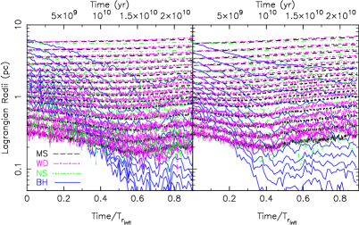
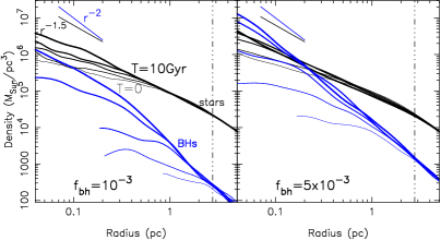
Figure 1.— Top panels show the Lagrangian radii for the four stellar species during the $N$-body simulations with BH number fractions: $f_{\rm bh}=10^{-3}$ (left panels) and $f_{\rm bh}=5\times 10^{-3}$ (right panels). Top tick-marks give times after scaling to the Milky Way; we adopted a relaxation time at the Sgr A* influence radius of $25$ Gyr (e.g., Merritt, 2010). Bottom panels show the density profile of stars and BHs at $t=(0,~{}2.5,~{}5,~{}7.5,~{}10)$Gyr; central density increases with time. Clearly, even after a time of order $10~{}$Gyr, the distribution of stars and BHs in our models can be very different from the relaxed multi-mass models that are often used to describe the center of galaxies. Vertical line marks the MBH influence radius.

Figure 2.— Evolution of the density slope, $\gamma\equiv-d\log\rho/d\log r$, of the main-sequence density profile in multi mass $N-$body models (central and right panels), compared to a model with only one mass component (left panel). The continue curves show profiles at $(0.2,~{}0.4,~{}0.6,~{}0.8,~{}1)\times T_{r_{\rm infl}}$; increasing line width corresponds to increasing time. The dashed curve corresponds to the initial model. Adding a BH component accelerates the growth of a density cusp in the stellar component. However the time to regrow a cusp in these models is always longer than $0.2T_{r_{\rm infl}}$, i.e., ${\rm 5Gyr}$ when scaled to the Milky Way, a time longer than the mean stellar age of the Galactic NC.

2.1. Evolution toward the steady state

We consider four mass groups representing main sequence stars (MSs), white dwarfs (WDs), neutron stars (NSs) and BHs. After the quasi steady-state is attained, the stars are expected to follow a central $r^{-3/2}$ cusp, while the heavier particles will have a steeper $r^{-2}$ density profile (e.g., Alexander, 2005). We assume that all species have the same phase space distribution initially as it would be expected for a violently relaxed system. This is the assumption that was made in most previous papers (e.g., Freitag et al., 2006; Hopman & Alexander, 2006; Merritt, 2010). We specify the mass ratio, $m_{\rm wd}/m_{\star}=0.6$, $m_{\rm ns}/m_{\star}=1.4$, $m_{\rm bh}/m_{\star}=10$, between the mass group particles and respective number fractions, $f_{\rm wd}=N_{\rm wd}/N_{\star}$, $f_{\rm ns}=N_{\rm ns}/N_{\star}$, $f_{\rm bh}=N_{\rm bh}/N_{\star}$.

Number counts of the old stellar population at the GC are consistent with a density profile of stars that is flat or slowly rising toward the MBH inside its sphere of influence and within a radius of roughly $\sim 0.5~{}$pc (Buchholz et al., 2009; Do et al., 2009; Bartko et al., 2010). Outside this radius the density falls off as $r^{-2}$. Merritt (2010) showed that a core of size $\sim 0.5~{}$pc is a natural consequence of two-body relaxation acting over $10~{}$Gyr, starting from a core of radius $\sim 1~{}$pc. It is therefore of interest to study the evolution of the BH distribution for a time of order the age of the Galaxy and starting from a density distribution with a parsec-scale core. We adopt the truncated broken-power-law model:

$$\rho(r)=\rho_{0}\left(\frac{r}{r_{0}}\right)^{-\gamma_{i}}\left[1+\left(\frac{r}{r_{0}}\right)^{\alpha}\right]^{(\gamma_{i}-\gamma_{e})/{\alpha}}\zeta(r/r_{\rm cut})~{},$$ (1)

were $\zeta(x)=\frac{2}{\mathrm{sech}(x)+\mathrm{cosh}(x)}$, $\alpha$ is a parameter that defines the transition strength between inner and outer power laws, $r_{0}$ is the scale radius and $r_{\rm cut}$ is the truncation radius of the model. The values adopted for these parameters were: $r_{0}=1.5$pc, $\alpha=4$, $\gamma_{e}=1.8$ and $r_{\rm cut}=6$pc. We included a central MBH of mass $M_{\bullet}=4\times 10^{6}~{}M_{\odot}$ and generated the models $N$-body representations via numerically calculated distribution functions. The central slope was set to $\gamma_{i}=0.6$, the smallest density slope index consistent with an isotropic distribution for the adopted density model and potential.

The normalizing factor $\rho_{0}$ was chosen in such a way that the corresponding density profile reproduces the coreless density model:

$$\rho(r)=1.5\times 10^{5}\left(\frac{r}{1{\rm pc}}\right)^{-1.8}M_{\odot}{\rm pc}^{-3}$$ (2)

outside the core. This choice of normalizing constant gives a mass density at $1~{}$pc similar to what it is inferred from observations (e.g., Oh et al., 2009), and gives a total mass in stars within this radius of $\sim 1.6\times 10^{6}~{}M_{\odot}$. The fact that our models are directly scalable to the observed stellar density distribution of stars at the GC is important if we want to draw conclusions about the current dynamical state of stars and BHs at the GC. We note, for example, that the merger models of Gualandris & Merritt (2012) had core radii that were substantially larger than the MBH influence radius. As also noted by these authors, this simple fact precluded a unique scaling of their models to the Milky Way – at least in the Galaxy’s current state in which the stellar core size ($\sim 0.5~{}$pc) is much smaller than the Sgr A* influence radius ($\sim 3~{}$pc).

We run three simulations with $N=132$k particles. These simulations differ with each other by the adopted number fractions of the four mass groups: (i) $f_{\rm wd}=f_{\rm ns}=f_{\rm bh}=0$; (ii) $f_{\rm wd}=10^{-1}$, $f_{\rm ns}=10^{-2}$, $f_{\rm bh}=10^{-3}$; (iii) $f_{\rm wd}=2\times 10^{-1}$, $f_{\rm ns}=2\times 10^{-2}$, $f_{\rm bh}=5\times 10^{-3}$. The latter two set of values correspond roughly to the number fractions expected from a standard and from a top-heavy IMF respectively. A fraction $f_{\rm bh}=10^{-3}$ is what expected for a standard (Kroupa-like) IMF and it is the value typically adopted in previous studies (e.g. Hopman & Alexander, 2005, 2006). Although a larger fraction of stellar remnants might be possible, for instance if the Galactic center always obeyed a top heavy initial mass function, the observationally constrained mass-to-light ratio of the inner parsec limits the BH fraction to only a few percent and it is more consistent with a ratio and a total mass of BHs predicted by a standard IMF (Löckmann et al., 2010). We evolved these systems for a time equal to the relaxation time, $T_{r_{\rm infl}}$, computed at the sphere of influence of the MBH. The relaxation time was evaluated using the expression (Spitzer, 1987):

$$T_{r}=\frac{0.34\sigma(r)^{3}}{G^{2}<m>{\rm ln}\Lambda\rho(r)}$$ (3)

with $\rho$ the total local mass density, and $<m>$ the average particle mass. For the Coulomb logarithm we used $\ln\Lambda=\ln\left(r_{\rm infl}\sigma^{2}/2Gm_{\star}\right)\approx 10$, with $\sigma$ the 1d velocity dispersion outside $r_{\rm infl}=GM_{\bullet}/\sigma^{2}$.

To scale the $N-$body time length to the Milky Way we consider that the relaxation time at the influence radius of Sgr A*, $r_{\rm infl}\approx 3$pc, is $T_{r_{\rm infl}}\approx 25~{}$Gyr, assuming a stellar mass of $1M_{\odot}$ (Merritt, 2010; Antonini & Merritt, 2012). Thus, when scaling to the GC, a time of $0.4T_{r_{\rm infl}}$ corresponds to roughly $10~{}$Gyr.

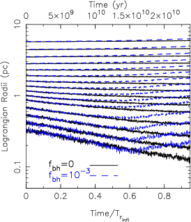
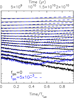
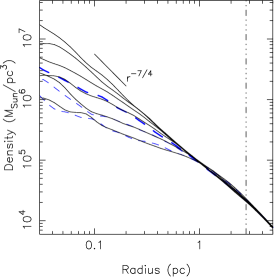
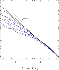
Figure 3.— Evolution of the $f_{\rm bh}=0$ model Lagrangian radii and density profile compared to the evolution of models with $f_{\rm bh}=10^{-3}$ (left panel) and $f_{\rm bh}=5\times 10^{-3}$ (right panel) . In the bottom panels the density profile is plotted at $t=(0,~{}5,~{}10,~{}15,~{}20,~{}25)$Gyr of evolution. The blue-dashed curves give the evolution of the stellar distribution Lagrangian radii in the models with BHs and the bottom panels show the respective stellar density profiles at $t=(0,~{}5,~{}10)$Gyr. Over a time of order $10~{}$Gyr the evolution of the density profile of stars in the $f_{\rm bh}=10^{-3}$ model is not much affected by the presence of the BHs. In the model with $f_{\rm bh}=5\times 10^{-3}$ the evolution toward the steady state is faster and after $10$Gyr the stars have formed a cusp. Vertical lines give the MBH influence radius.

We evolved the initial conditions with the direct $N-$body integrator $\phi$GRAPEch (Harfst et al., 2008). The code implements a fourth-order Hermite integrator with a predictor-corrector scheme and hierarchical time stepping. The code combines hardware-accelerated computation of pairwise interparticle forces (using the Sapporo library which emulates the GRAPE interface utilizing GPU boards, Gaburov et. al., 2009) with a high-accuracy chain regularization algorithm to follow the dynamical interactions of field particles with the central MBH particle. The chain radius was set to $10^{-2}$pc and we used a softening $\epsilon=10^{-6}~{}$pc. The relative error in total energy was typically $\sim 10^{-4}$ for the accuracy parameter $\eta=0.01$.

Figure 1 shows the evolution of the $N$-body models over one relaxation time. The heavy particles segregate to the center owing dynamical friction. After the central mass density of BHs becomes comparable to the density in the other species, the evolution of the BH population starts being dominated by BH-BH self interactions; at the same time the lighter species evolve in response to dynamical heating from the BHs, which causes the local stellar densities to decrease and Lagrangian radii to expand. As shown below, the same heating rapidly converts the initial density profile into a steeply rising density cusp with slope, $\gamma\equiv-d\log\rho/d\log r\approx 3/2$. The inclusion of a BH population has therefore two effects on the main sequence population: it lowers the stellar densities and at the same time it accelerates the evolution of the density of stars toward the $\gamma=3/2$ steady-state form.

The lower panels of Figure 1 display the density profile of stars and BHs over $10~{}$Gyr of evolution. These plots show that, starting with a fraction of BHs that corresponds to a standard IMF: (1) after $\sim 10$Gyr the density of BHs can remain well below the density of stars at all radii; (2) even after 10 Gyr of evolution, the density distribution of stars looks very different from what expected for a dynamically relaxed population around a MBH. These findings are in agreement with the Fokker-Plank simulations of Merritt (2010) but in contrast with more recent claims that mass segregation can rebuild a stellar cusp in a relatively small fraction of the Hubble time (e.g., Preto & Amaro-Seoane (2010), and the Introduction of Amaro-Seoane & Xian (2013)). Figure 2 displays the evolution of the radial profile of the density profile slope. Comparing the evolution observed in models with and without BHs we see that a cusp in the main-sequence population develops earlier in models with BHs. Figure 2 shows that for $f_{\rm bh}=10^{-3}$ and $f_{\rm bh}=5\times 10^{-3}$ a stellar cusp only develops after $\sim 0.6T_{r_{\rm infl}}$ and $\sim 0.4T_{r_{\rm infl}}$ respectively. Therefore over the timescales ($\lesssim 10~{}$Gyr) and radii ($r\gtrsim 0.01$pc) of relevance, the inclusion of a BH population has little or even no influence on the evolution of the lighter populations. This latter point is more clearly demonstrated in Figure 3 which directly compares the Lagrangian radii evolution of our $f_{\rm bh}=0$ model with models with BHs. The stellar populations evolve similarly in these models independently on $f_{\rm bh}$ until approximately $0.6$ and $0.4\times T_{r_{\rm infl}}$ for $f_{\rm bh}=10^{-3}$ and $5\times 10^{-3}$ respectively. After this time, heating of the lighter species by the heavy particles starts becoming important causing the density of the former to decrease and deviate from the evolution observed in the single-mass component model. However, the transition to this phase clearly occurs after the models have been already evolved for a time comparable (for $f_{\rm bh}=5\times 10^{-3}$) or longer (for $f_{\rm bh}=10^{-3}$) than the age of the Galactic NC .

Given the results of the simulations presented in this section, we can schematically divide mass-segregation in two phases: in phase (1) the density of BHs is smaller than the density of stars and the models evolve mainly due to scattering off the stars – the BHs inpiral to the center due to dynamical friction, and the stellar distribution relaxes as in a single mass component model. In phase (2), when the density of BHs becomes comparable and larger than the density of stars, BHs and stars evolve due to scattering off the BHs which causes the models to rapidly evolve toward the steady state.

Perhaps, the most interesting aspect of our simulations is the long timescale required by the BH population to segregate to center through dynamical friction (phase 1 above) and reach a (nearly) steady state distribution – a time comparable to the relaxation time as defined by the dominant stellar population. In what follows we show that these predictions agree well with the evolution expected on the basis of theoretical arguments.

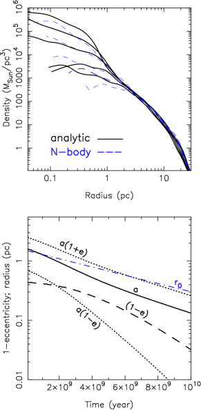
Figure 4.— The top panel shows the evolution of the density of $10~{}M_{\odot}$ BHs due to dynamical friction against the field stars. The density profiles are shown at $t=(0,2,4,6,8)~{}$Gyr. Blue-dashed curves were obtained via direct $N$-body simulations; black-solid curves correspond to the results of our semi-analytical model in which the frictional force was computed using Equation (2.2), which accounts for the contribution of the fast-moving stars to the frictional force. Bottom panel shows the evolution of angular momentum ($1-e$) and semi-major axis ($a$) of a $10M_{\odot}$ BH in our GC model. Blue-dot-dashed curve shows the break radius evolution of the background model. Note that as the BH reaches roughly $r_{0}/2$ its orbital radius migrates inward on a timescale similar to that over which the core in the background density evolves due to two-body relaxation.

2.2. Analytical estimates

In order to understand the evolution of the distribution of BHs observed in the $N$-body simulations, we evolved the population of massive remnants using an analytical estimate for the dynamical friction coefficient. The stellar background was represented as an analytic potential which was also let evolve in time accordingly to the evolution observed in the stellar distribution during the $N$-body simulations.

We began by generating random samples of positions and velocities from the isotropic distribution function corresponding to the density model of Equation (1). The orbital equations of motion were then integrated forward in time in the evolving smooth stellar potential and including a term which describes the orbital energy dissipation due to dynamical friction. The dynamical friction acceleration was computed using the expression:

$$\boldsymbol{a_{\rm fr}} \approx -4\pi G^{2}m_{\rm bh}\rho(r)\frac{\boldsymbol{v}}{v^{3}}$$

$$\times{\Big{(}}{\rm ln}\Lambda\int_{0}^{v}dv_{\star}4\pi f(v_{\star})v_{\star}^{2}~{}$$

$$+\int^{{\infty}}_{v}dv_{\star}4\pi f(v_{\star})v_{\star}^{2}\left[{\rm ln}\left(\frac{v_{\star}+v}{v_{\star}-v}\right)-2\frac{v}{v_{\star}}\right]\Big{)},$$

with $v$ the velocity of the inspiraling BH and $f(v_{\star})$ the velocity distribution of field stars. The second term in parenthesis of Equation (2.2) represents the frictional force due to stars moving faster than the test mass. Such “non-dominant” terms are neglected in the standard Fokker-Plank treatment in which the dynamical friction coefficient is obtained by integrating only over field stars with velocity smaller than that of the test particle (e.g., Hopman & Alexander, 2006; Alexander & Hopman, 2009; Merritt, 2010). Antonini & Merritt (2012) showed that this approximation breaks down in a shallow density profile of stars around a MBH where such terms can become dominant, as there are a few or even no particles moving more slowly than the local circular velocity.

The $N$-body integrations show that the stellar distribution changes with time in a quasi-self-similar way – the stellar density profile break radius shrinks progressively with time while the outer profile slope is maintained roughly unchanged. In order to account for such evolution, we computed at each time the best fitting density model of Equation (1) to the density profile of stars in the $N$-body system at that time. We used this density model to compute gravitational potential, distribution function and corresponding dynamical friction coefficient. This procedure allowed us to include the evolution of the stellar background when evolving the BH population. Our integrations are unique in the sense that they are the first including at the same time: (i) a correct estimate of the dynamical friction coefficient, which takes into account the contribution of stars moving faster than the inspiraling BH, and (ii) a realistic treatment of the evolution of the stellar background under the influence of gravitational encounters. However, since our analysis does not take into account BH-BH self interactions, our integrations are only valid until the density of BHs remains well below the density of stars. In this respect, our approach is limited to the early evolution of the system, when the BHs only represent a negligible perturbation on the evolution of the light component.

The upper panel of Figure 4 shows the density profile of BHs obtained from the semi-analytical modeling described above and compares it to the results from the direct $N$-body simulation with BH fraction $f_{\rm bh}=10^{-3}$. The central density of BHs increases with time at a rate which is comparable in the two models. The plot shows that the spatial distribution of stellar-mass BHs near the GC might not have reached a steady state form – at least if their initial distribution was similar to what used in our models. In fact, even after a time of $\approx 8$Gyr the central density of BHs is still substantially lower than the density of stars. As our analysis demonstrates, the persistence of such low densities of BHs is a direct consequence of the long timescale of inspiral in a density core near a MBH. This latter point is illustrated in the lower panel of Figure 4 which shows the trajectory of a $10~{}M_{\odot}$ BH at the GC. The rate of orbital decay slows down as the BH reaches $\approx r_{0}/2$, due to the lack of low-velocity stars in the core. After the BH reaches this radius dynamical friction becomes very inefficient and the decay of the BH orbit proceeds at a rate which is comparable to the rate at which the core radius in the stellar distribution shrinks due to gravitational encounters — a time of order the relaxation time of the nucleus.

2.3. Comparison with recent work

In this section we used direct $N$-body integrations as well as analytic models to describe the evolution of multi-mass models of the Milky Way NC characterized by an initial parsec-scale core in the density distribution. Calculations similar to those described here were recently performed by Preto & Amaro-Seoane (2010) and Gualandris & Merritt (2012).

Preto & Amaro-Seoane (2010) studied the evolution of models with two mass species: stars and BHs. These authors concluded that mass segregation of the heavy component speeds up cusp growth in the lighter component by factors up to 10 in comparison with the single-mass case. This conclusion is somewhat in agreement with the results of our simulations which also show that a stellar cusp, extending out to roughly $r_{\rm infl}$, regrows faster in models with BHs (e.g., Figure 2). However, for realistic numbers of BHs we find that the timescale of cusp regrowth is only a factor of two shorter than in the single-mass component models. Preto & Amaro-Seoane (2010) argued that the time scales associated with cusp regrowth are clearly shorter than the Hubble time for nuclei similar to that of the Milky Way – even though the relaxation time, as estimated for a single mass stellar distribution, exceeds one Hubble time. Based on our study we conclude instead that over one Hubble time and if a standard IMF is adopted adding a heavy component has relatively little effect on the evolution of the main-sequence component (e.g., Figure 3). Even for a top-heavy IMF, which results in initial larger densities of BHs, the time for cusp regrowth is longer than the mean stellar age in the Galactic center ($\sim 5~{}$Gyr). The reason for this is that due to the inefficient dynamical friction force in a density core around a MBH, the central density of BHs remains well below the density of stars for a time of order the relaxation time of the nucleus. The time required to regrow a cusp in the stellar distribution appears to be longer than the Hubble time for galaxies similar to the Milky Way.

Gualandris & Merritt (2012) simulated the merger between galaxies with MBHs containing four mass groups, representative of old stellar populations. They followed the evolution of the merger products for about three relaxation times and found that the density cores formed during the galaxy mergers persisted, and that the distribution of the stellar-mass black holes evolved “against an essentially fixed stellar background”. Gualandris & Merritt (2012) also integrated the exact same Fokker-Planck models as in Preto & Amaro-Seoane (2010) and argued that the accelerated cusp growth described by these latter authors is seen to be present only at small radii, $r\lesssim 0.05~{}{r_{\rm infl}}$. At radii larger than these adding the BHs has the effect of lowering the density of the stellar component at all times. Gualandris & Merritt (2012) argued that Preto & Amaro-Seoane (2010) were misled by looking at the very-small-radius regime in their Fokker-Plank solutions, where the cusp in the main sequence component stands out. Our study shows that the BH population has indeed two effects on the main-sequence population: it lowers the “mean” density of stars (the point stressed in Gualandris & Merritt, 2012), and it accelerates the redistribution of the stars in phase-space, toward the $\gamma=3/2$ steady-state (as found in Preto & Amaro-Seoane, 2010). So in a sense, the BHs both “create” and “destroy” a cusp: although the presence of a BH population can significantly accelerate the timescale of cusp regrowth in the stellar distribution, the scattering off the heavy (BH) component causes the density of stars to decrease at radii larger than $\sim 0.05~{}{r_{\rm infl}}$.

3. Globular cluster merger model; evolution Time Scales

In the previous section we have shown that due to the long timescales of evolution, the current distribution of BHs and stars at the center of galaxies similar to the Milky Way should be considered very uncertain. In these and more massive galaxies the current distribution of stars and BHs can still reflect their initial conditions and the processes that have lead to the formation and evolution of their central NC. This conclusion suggests that standard mass-segregation models, which assume the same initial phase space distribution for BHs and stars, can lead to misleading conclusions regarding the current dynamical state of galactic nuclei and motivates studies that start from initial conditions which correspond to well-defined physical models.

In what follows, we present a set of $N$-body experiments which were designed to understand the distribution of stars and BHs in galactic nuclei formed via repeated merger of massive stellar clusters – a formation model which has been shown to be very successful in reproducing the observed properties and scaling relations of nuclear star clusters (e.g., Turner et al., 2012; Antonini, 2013). We begin here with discussing the relevant timescales of the problem, including the characteristic orbital decay time of massive clusters in the inner regions of galaxies, and the relaxation timescales of galactic nuclei and globular clusters.

3.1. Globular Clusters decay time.

Sufficiently massive and compact clusters can decay towards their parent galaxy central region in a time much shorter than the Hubble time. An approximation of the time for clusters (within the half mass radius of the stellar bulge) to spiral to the center is given by (Antonini et al., 2012):

$$\Delta t_{h}\approx 3\times 10^{10}{\rm yr}~{}~{}\tilde{R}_{eff}^{1.75}\tilde{m}^{-1}~{}.$$ (5)

with $\tilde{R}_{eff}$ the galactic effective radius in kpc, and $\tilde{m}$ the globular cluster mass in units of $10^{6}~{}M_{\odot}$. Within $\Delta t_{h}$ the forming nucleus has a luminosity comparable to that of the surviving clusters. Equation (5) predicts that a significant fraction of the globular cluster population in faint and intermediate luminosity stellar spheroids would have spiraled to the center by now, while in giant ellipticals, due to their larger characteristic radii, the time required to grow a NC might be longer than $10^{10}~{}$yr. We stress that the inspiral time obtained using Equation (5) gives only a crude approximation (likely an overestimate) of the real dynamical friction time scale. Nevertheless it is reasonable to draw the conclusion that the observed lack of nuclei in galaxies more massive than about $10^{10}~{}M_{\odot}$ could be due to the longer infall times in these galaxies, due to their larger values of $R_{eff}$. Figure 5 presents a test of this idea. This figure gives effective radii versus masses, $M_{gal}$, for galaxies belonging to the Virgo cluster that either have (filled black circles) or do not have (star symbols) a central NC. Dashed curves give the value of $R_{eff}$ obtained by setting $\Delta t_{h}=10^{10}~{}$yr in Equation (5) and adopting various masses of the sinking object. The figure shows that only in galaxies with $M_{gal}\lesssim 10^{10}~{}M_{\odot}$, massive globular clusters would have enough time to spiral into the center, merge and form a compact nucleus. The observed absence of compact nuclei in giant ellipticals could be therefore interpreted as a consequence of the long dynamical friction time scale of globular clusters in these galaxies.

We add that the density profile of stars in giant ellipticals is often observed to be flat or slowly rising inside the influence radius of the MBH. As shown in Section 2 this implies a very long dynamical friction time scale inside the MBH influence radius due to the absence of stars moving more slowly than the local circular velocity (Antonini & Merritt, 2012). Massive clusters orbiting within the core of a giant elliptical galaxy do not reach the center even after $10^{10}~{}$yr. In addition, due to the strong tidal field produced by the MBH, globular clusters can only transport little mass to the very central region of the galaxy. Both these effects, i.e. long inspiral times and little mass transported to the center, have been suggested to suppress the formation of NCs in bright galaxies, in agreement with observations (Antonini, 2013).

Figure 5.— effective radii ($R_{eff}$) of galaxies plotted against their masses ($M_{gal}$). Filled circles and star symbols represent respectively nucleated and un-nucleated galaxies that belong to the Virgo galaxy cluster (Côté et al., 2006). Dots are data from Forbes et al. (2008). Vertical line gives the value of the mass ($M_{gal}\approx 10^{10.5}~{}M_{\odot}$) which approximately set the transition between nucleated galaxies ($M_{gal}<10^{10.5}~{}M_{\odot}$), and MBH dominated galaxies ($M_{gal}>10^{10.5}~{}M_{\odot}$) (Côté et al., 2006). Dashed-horizontal curves give the value of $R_{eff}$ obtained by setting $\Delta t_{h}=10^{10}~{}$ in Equation (5) and adopting various masses of the sinking objects. The large effective radii of massive galaxies give time scales for inspiral that are usually longer than one Hubble time. The observed lack of nuclei in massive galaxies could be explained as a consequence of the longer infall times in these galaxies, due to their large effective radii.

3.2. Nuclear star clusters relaxation time

A useful reference time for our study is the relaxation time computed at the radius containing half of the mass of the system, $R$. Setting ${\rm ln}\Lambda=12$, and ignoring the possible presence of a MBH, the half mass relaxation time is:

$$T_{h}=2.1\times 10^{5}\frac{\left[r_{h}(\rm pc)\right]^{3/2}N^{1/2}}{(m/M_{\odot})^{1/2}}\frac{10}{\ln(0.4N)}{\rm yr}~{},$$ (6)

where $N$ is the total number of stars.

In the absence of a MBH, collisional relaxation leads to mass segregation and core collapse. In a pre-existing NC, the presence of a MBH inhibits core collapse, causing instead the formation of a Bahcall-Wolf cusp, $n\sim r^{-7/4}$, on the two-body relaxation time scale (Preto et al., 2004; Merritt, 2009). Nuclear clusters belonging to the Virgo galaxy cluster have half-mass relaxation time that scales with the total absolute magnitude of the host galaxy, $M_{B}$, as (Merritt, 2009):

$${\rm log}\left(T_{h}/{\rm yr}\right)=9.38-0.43(M_{B}+16)~{}.$$ (7)

Galaxies with luminosities less than $\sim 4\times 10^{8}~{}L_{\odot}$, have NCs with relaxation times that fall below $10~{}$Gyr. These galaxies have NCs with masses $\lesssim 10^{7}~{}M_{\odot}$ and half mass radii $r_{h}\lesssim 10~{}$pc. These limiting values appear close to those characterizing the Milky Way NC, suggesting that only spheroids fainter than the Milky Way have collisionally relaxed nuclei. Relaxation times for nuclei with masses $\gtrsim 10^{7}~{}M_{\odot}$ are therefore too long for assuming that they have reached a collisionally relaxed state, but they are still short enough that gravitational encounters would substantially affect their structure over the Hubble time. This is in agreement with the results of Section 2 and also appears to be consistent with absence of a Bahcall-Wolf cusp in the distribution of stars at the GC.

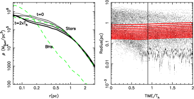
Figure 6.— Evolution of the cluster model during the initial $N$-body integrations used to realize the mass-segregated cluster models for Runs A1 and A2 (see Table 1). The left panel shows the evolution of the stellar density profile. Line thickness increases with time. The green-dashed curves give the density profile of stars and BHs used as initial conditions for the inspiral runs. Right panel gives the Lagrangian radii of the stellar component (red solid curves) and the BHs distance from the cluster center (black dots). The BHs segregate to the cluster core forming a dense sub-cluster in about one, half-mass relaxation time as defined by the stellar component. The stellar cluster slightly expands due to heating by the inspiraling BHs. Vertical line gives the time at which we extracted the initial conditions for the inspiral simulations.

3.3. Globular clusters relaxation time

Globular clusters with $N\sim 10^{6-7}$ have relaxation times $T_{h}\sim 10^{9-10}~{}$yr. Most Galactic globular clusters are therefore relaxed systems. The time scale required for the BH population to segregate to cluster center and there form a subcluster dynamically decoupled from the host stellar cluster is approximately the core collapse time for the initial BH cluster (e.g., Banerjee et al., 2010):

$$T_{ms}\approx\frac{m}{m_{bh}}T_{cc}~{},$$ (8)

where ${m_{bh}}$ is the mass of a stellar black hole and $T_{cc}$ is the core collapse time of the host stellar cluster which is about $T_{cc}\approx 15\times T_{h}$ for a Plummer model. After $\sim T_{ms}$ the central density of BHs becomes large enough that BH-BH binary formation takes place through three or four body interactions (Heggie & Hut, 2003). The formed BH binaries then “harden” through repeated super-elastic encounters that lead to the ejection of BHs from the cluster core until eventually only a few BHs are left (e.g., Banerjee et al., 2010).

In galaxies similar tot he Milky Way, stellar clusters with masses $\gtrsim 10^{6}~{}M_{\odot}$ and starting from a galactocentric radius of $1~{}$kpc have orbital decay times due to dynamical friction less than $\lesssim 3~{}$Gyr (Equation5). The clusters dynamical friction time is therefore typically long compared to the timescale over which the BHs would segregate to center of the cluster.

It is possible that the BH population will evaporate through super elastic encounters before the cluster reaches the center of the galaxy. This could lead to the formation of a NC with a much smaller abundance of BHs relative to stars than what predicted by standard initial mass functions. On the other hand, for massive clusters after the BHs are already segregated to the center, the encounter driven evaporation time scale of the BH sub-cluster typically requires an additional few Gyr of evolution to complete  (Dowing et al., 2010, 2011). Moreover, recent theoretical studies (Morscher et al., 2013; Sippe & Hurley, 2013), together with several observational evidences (Maccarone et al., 2007; Brassington et al., 2010; Maccarone et al., 2011; Strader et al., 2012), show that old globular clusters may still contain hundreds of stellar BHs at present which suggests that BH depletion might not be as efficient as previously thought. This indicates that for many large clusters (the ones most relevant to NC formation), most of the BHs will not be ejected before inspiral has occurred. The above arguments convinced us that the inspiral of massive clusters in the central region of the Galaxy could serve as a continuos source term of BHs in these regions.

Table 1Initial Modles

${\rm Run}$	$N_{\rm gal}$	$N_{\rm cl,\star}$	$N_{\rm cl,bh}$	# of infalls	Galaxy model
A1	$1\times 10^{6}$	45720	240	1	Model 1
A2	$1.5\times 10^{6}$	45720	240	1	Model 2
B	$4.6\times 10^{5}$	5715	33	12	Model 1
C	$4.6\times 10^{5}$	5715	100	12	Model 1

4. Numerical set-up

4.1. Initial conditions and numerical method

In Antonini et al. (2012) we used $N$-body simulations to study how the presence of a MBH at the center of the Milky Way impacts the globular cluster merger hypothesis for the formation of its NC. We determined the properties of the stellar distribution in a galactic nucleus forming through the infall and merging of globular clusters. We showed that a model in which a large fraction of the mass of the Milky Way NC arose from infalling globular clusters is consistent with existing observational constraints. Here we replaced the single-mass globular cluster models of Antonini et al. (2012) with systems containing (in addition to the stellar component) a remnant population of BHs.

These simulations were performed by using $\phi$GRAPE (Harfst et al., 2006), a direct-summation code optimized for running on GRAPE accelerators (Makino & Taiji, 1998). This integrator is equivalent to $\phi$GRAPEch which we used in Section 2, but without the regularized chain. The accuracy and performance of the code are set by the time-step parameter $\eta$ and the softening length $\epsilon$. We used a Plummer softening for the gravitational force between particles, and we did not model binary formation in the calculation reported below. We set $\eta=0.01$ and $\epsilon=10^{-4}$pc. With these choices, energy conservation was typically $\;\hbox to0.0pt{\lower 2.5pt\hbox{$\sim$}\hss}\raise 1.5pt\hbox{$<$}\;0.01\%$ during each merging event. The simulations were carried out using the 32-node GRAPE cluster at the Rochester Institute of Technology, and also on Tesla C2050 graphics processing units on the Sunnyvale cluster at the Canadian Institute for Theoretical Astrophysics. In the latter integrations, $\phi$GRAPE was used in serial mode with sapporo (Gaburov et. al., 2009). Each simulation required between $3$ to $4$ months total of computational time.

Table 1 summarizes the parameters of the $N-$body models. We performed four simulations. Runs A1 and A2 are high resolution simulations ($N\sim 10^{6}$) that explore the dynamics of one single globular cluster inspiral. In simulations B and C the total number of $N$-body particles was greatly reduced in order to more efficiently follow the consecutive inspiral and merger of $12$ dynamically evolved clusters. In these latter simulations each inspiral simulation was started after the stars from the previously disrupted cluster were set to a state of collionless dynamical equilibrium and the number of BHs in the cluster remnant dropped to $<10$. This corresponds to a time of $1-3\times 10^{7}$yr for each inspiral event to complete, with the longer times corresponding to the earlier infalling clusters. The clusters were initially placed on circular orbits at a distance of $20$ pc from the center. The choice of circular orbits was motivated by the well-known effect of orbital circularization due to dynamical friction (e.g., Casertano et al., 1987; Hashimoto et al., 2003). In the consecutive merger simulations (runs B and C), in order not to favor any particular direction for the inspiral, the orbital angular momenta were selected in the following way: the surface of a sphere can be tessellated by means of 12 regular pentagons, the centers of which form a regular dodecahedron inscribed in the sphere. The coordinates of the centers of these pentagons were identified with the tips of the 12 orbital angular momentum vectors. In this way, the inclination and longitude of ascending node of each initial orbit were determined.

4.2. Galaxy models

We adopted two different $N-$body models to represent the central region of the Galaxy. Model 1 is obtained by an inner extrapolation of the observed density profile of stars in the Galactic nuclear bulge outside $10~{}$pc. In these regions the Galaxy is dominated by the presence of the nuclear stellar disk which is characterized by a flat density profile. Accordingly, we adopted the truncated shallow power-law density model:

$$\rho_{\rm gx,1}(r)=\tilde{\rho}\left(\frac{r}{\tilde{r}}\right)^{-\gamma}\text{sech}\left(\frac{r}{r_{\rm cut}}\right)$$ (9)

where $\tilde{\rho}=400$M${}_{\odot}/$pc³ is the density at $\tilde{r}=10$pc, and the truncation radius is $r_{\rm cut}=20~{}$pc. Hence, the initial conditions for Model 1 does not include a preexisting NC and they correspond to a shallow density cusp around a central MBH.

Model 2 was obtained by the superposition of the density model of Equation (9) and a broken power law model representing a NC:

$$\rho_{\rm gx,2}(r) = \rho_{\rm gx,1}(r)$$ (10)

$$+ \rho_{b}\left(\frac{r}{r_{b}}\right)^{-\gamma_{i}}\left[1+\left(\frac{r}{r_{b}}\right)^{\alpha}\right]^{(\gamma_{i}-\beta)/\alpha}\text{sech}\left(\frac{r}{r_{\rm cut}}\right),~{}~{}~{}~{}$$

with $\rho_{b}=4.1\times 10^{4}\text{M}_{\odot}/\text{pc}^{3}$, $r_{b}=1.5~{}$pc, $\gamma_{i}=0.5$, $\beta=1.9$, $\alpha=3.73$ and $r_{\rm cut}=20~{}$pc. This model corresponds approximately to the best fitting density profile of the simulations end-product of Antonini et al. (2012).

In both Model 1 and Model 2 we included a central MBH of mass $M_{\bullet}=4\times 10^{6}~{}M_{\odot}$ and we generated their $N$-body representations via numerically calculated distribution functions.

4.3. Star clusters model

We generated our globular cluster initial conditions following the same procedure described in Antonini et al. (2012), where a detailed description of the initial conditions of the clusters can be found. In brief, the clusters are started on circular orbits of radius $r=20~{}$pc, and their initial masses and radii are set up in such a way as to be consistent with the galactic tidal field at that radius. The clusters are King models (King, 1962) with central (King) potential $W_{0}$=5.8, core radius $r_{k}$=0.5 pc, and central velocity dispersion $\sigma_{K}=35~{}{\rm km~{}s^{-1}}$. With this set of parameters the truncated mass of the clusters was $m_{\rm cl}\approx 1.1\times 10^{6}~{}M_{\odot}$.

To these models we added a heavier mass group representing a population of stellar BHs. The relative values of the particle masses was 1:10. These represent respectively one solar mass stars and $10~{}M_{\odot}$ BHs. The two mass groups had the same initial phase-space distribution. Standard population synthesis models predict that about $1\%$ of the total mass in a stellar system will be in BHs, top heavy mass functions result in about five times more BHs. Accordingly, in our initial models the total mass in BHs was $10^{-2}$ and $5\times 10^{-2}$ times $4\times 10^{6}M_{\odot}$ (the mass of the non-truncated King model) for run A-B and C (Table 1) respectively. The choice of scaling the total number of BHs to the initial non-truncated cluster mass is based on the fact that when the cluster reaches $100~{}$pc (roughly the radius at which our models start to be tidally truncated) mass segregation is likely to have already occurred. under these circumstances, tidal stripping will preferentially remove stars from the outer part of the system, leading to an overabundance of BHs with respect to standard mass functions (Banerjee & Kroupa, 2011). In addition, this choice resulted in a sufficiently good statistics for the remnants population. The effect of varying the initial mass in stellar BHs and their initial dynamical state inside the clusters will be investigated in a future paper.

The mass-segregated cluster models were then created via $N$-body integrations, starting from the cluster equilibrium models. Figure 6 gives the evolution of the two mass components during these integrations. We let the system evolve for a few relaxation times as defined by Equation (7). The stellar BHs accumulate toward the center and by approximately one half-mass relaxation times their distribution appears to have reached an approximately steady state. At the same time the density profile defined by the stellar component undergoes a slow expansion due to heating by the BHs.

5. Results

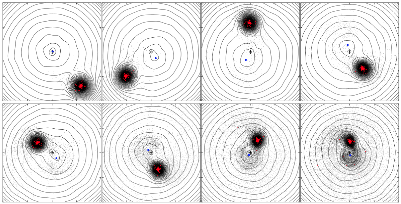
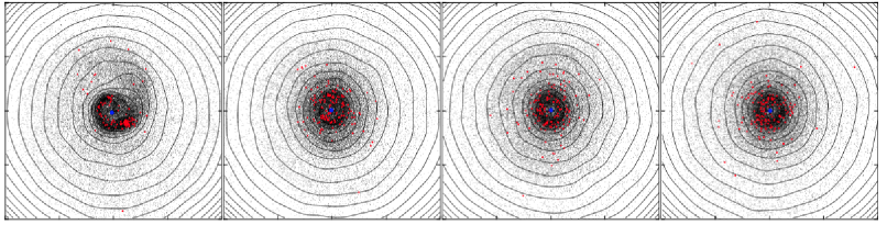
Figure 7.— Inspiral of a $\sim 10^{6}~{}M_{\odot}$ globular cluster in a Milky Way model. The linear size of each box is $20~{}$pc; the time separation between each snapshot is $5\times 10^{5}~{}$yr. The blue filled circle marks the galactic MBH position. Curves show the contours of the projected density of the background galaxy. Red points represent the globular cluster BHs; black dots the cluster stars.

Figure 8.— Time evolution of galactocentric radius (upper panels) and bound mass (lower panels) of the globular cluster models in runs A1 and A2 (see Table 1). In the lower panels we show separately the bound mass in BHs (curve starting at $6\times 10^{4}M_{\odot}$) and in stars (curve starting at $1.1\times 10^{6}M_{\odot}$) Dashed curves in the upper panels give the galactocentric radii in the initial galaxy models containing $10^{4}$ and $10^{5}~{}M_{\odot}$.

Figure 9.— Density profile of BHs and stars at the end of the single inspiral simulations of Table 1. Upper panel corresponds to simulation A1 and lower panel to simulation A2. Density profiles are given after the BH cluster are artificially dispersed as described in the text. Insert panels show the corresponding cumulative number distributions of stellar BHs. Dotted curves give the density model of the initial galaxy models of Equation (9) and Equation (10). The density profile of the galaxy at the end of the simulation is shown as dashed curves. Up to $\sim 100$ BHs are migrated inside the inner $0.1-0.2~{}$pc of the galactic center.

5.1. Single inspiral simulations

Figure 7 shows surface density contours of the single inspiral simulation A1. After $\sim 10^{7}~{}$yr the stellar cluster is at about $5~{}$pc from the center; at these distances the disruption process due to tidal stress from the central MBH begins. Rapid removal of stars from the outer part of the cluster by the galaxy and MBH tidal fields unveils its mass-segregated BH cluster. Figure 8 shows the time evolution of radius and bound mass for the globular clusters in runs A1 and A2. Our cluster models rapidly evolve to a state of dark stellar cluster, i.e., a dense cluster dominated by dark stellar remnants (Banerjee & Kroupa, 2011). After this state is reached, due to the drop in the total cluster mass (see lower panels of Figure 8), the dynamical friction drag on the remaining BH cluster is largely suppressed, slowing down its orbital decay toward the center of the galaxy. Noticeable, due to the common motion around the system MBH-cluster center of mass, the MBH is significantly displaced from the galaxy center. More precisely, we found a maximum displacement of $\sim 5~{}$pc in run A1 and a somewhat smaller (maximum) displacement of $\sim 2~{}$pc in run A2.

Figure 8 shows that after the stellar clusters are disrupted, the remaining dark clusters have a bound mass of $\sim 2.7\times 10^{3}~{}M_{\odot}$ in simulation A1 and $1.7\times 10^{4}~{}M_{\odot}$ in simulation A2, corresponding to 9 and 67 BH particles respectively. The enhanced removal of stars and BHs decelerates the orbital evolution of the cluster due to its lower mass. During the inspiral after about $2\times 10^{7}~{}$yr the BH cluster core has collapsed to $\lesssim 0.05~{}$pc. This makes the central density much higher, which prevents the complete disruption of the BH cluster.

Assume that the cluster has reached a state of “thermal equilibrium” at the center, i.e., a state in which the stars and BHs are represented by lowered Maxwellians: $m_{\rm st}\sigma_{\rm st}^{2}=m_{\rm bh}\sigma_{\rm bh}^{2}$, with $\sigma_{\rm st}$ ($\sigma_{\rm bh}$) the central one-dimensional velocity dispersion of the stars (BHs). If a MBH of mass $M_{\bullet}$ is present at the center of the galaxy, disruption occurs at distance

$$r_{\mathrm{disr}}\approx 2\left(\frac{\sigma_{\mathrm{NC}}}{5\sigma_{K}}\right)^{2/3}\left(\frac{r_{\mathrm{infl}}}{r_{K}}\right)^{1/3}r_{K}~{},$$ (11)

from the MBH. Then the BH cluster tidal disruption radius will be smaller than that of the stellar cluster by a factor

$$\approx 0.3\left(\frac{1}{20}\frac{r_{K;\rm bh}}{r_{K;\rm st}}\right)^{2/3}\left(\frac{1}{10}\frac{m_{\rm bh}}{m_{\rm st}}\right)^{1/3},$$ (12)

which suggests that the BHs can end up being more centrally concentrated than the stars. A condition for this to happen is that the BH cluster must not evaporate before it has lost significant orbital energy by dynamical friction. In fact, the internal evolution of a compact BH cluster embedded in the extreme tidal field of the GC can proceed very rapidly and lead to the cluster complete dissolution on a short timescale, of order a few Myr (e.g., Banerjee & Kroupa, 2011; Gürkan et al., 2005). In our simulations the internal dynamical evolution of the clusters has been suppressed by giving a non-negligible softening radius to the cluster particles. In fact, the adopted integrator cannot treat the postcollapse evolution of the cluster, since we used a softened potential. Thus we terminated the simulation at $\approx 3\times 10^{7}$yr of evolution after the clusters have been fully depleted of stars and the remaining BH clusters underwent core-collapse.

The end-product spatial density profile and cumulative mass distribution of stars and BHs are given in Figure 9. In order to obtain the BH density profile we forced the unbinding of the remnant clusters after $10^{7}$yr of evolution. The unbinding of the clusters was induced by “turning off” the gravitational interaction terms between the BH cluster members and by letting the system evolve for about one crossing time. Although quite artificial, this procedure allowed us to account for the fact that the dissolution time of the cluster remnants is expected to be short relative to their dynamical friction timescale – in our models a $10^{4}M_{\odot}$ system starting from a galactocentric radius of $1$pc reaches a radius of $0.2~{}$pc after $10^{8}$yr. The BH clusters will dissolve on a timescale proportional to the half-mass relaxation time, $T_{ev}\approx 300\times T_{h}$ (Spitzer, 1987) (if we ignore the effect of the external tidal field); from Equation (6), using $r_{h}=0.1$pc (Figure 6), $N=1000$, and $m=10M_{\odot}$ we find $T_{ev}\approx 10^{7}$yr. We stress that since the current state of the art computational capability does not allow us to simulate the actual number and mass of stars and to calculate the internal evolution of the cluster, the densities of BHs obtained here should be only considered as approximate (likely an underestimate of the real density). Note also that it is unlikely that the core collapse phase of a BH cluster can lead to the formation of an intermediate mass black hole since any BH-BH merger will eject the remnant from the cluster via asymmetric emission of gravitational wave radiation before it can accrete other BHs or sourradning stars.

The number of BHs in our simulations, $N_{\rm BH,nb}(<r)$, was converted to a predicted number for a Milky Way model, using the approximate scaling:

$$N_{\rm bh}(<r)=N_{\rm BH,nb}(<r)\times\frac{4\times 10^{6}M_{\odot}}{10M_{\odot}}\frac{m_{\rm BH,nb}}{M_{\bullet}}$$ (13)

with the last factor at second term containing the masses in the units of the $N$-body code. The number of BHs transported in the inner $\sim 1~{}$pc is of order $100~{}$ in both A1 and A2. Our simulations result in a mass distribution characterized by a flat density core inside $\sim 2$pc in run A1 and $\sim 3$pc in run A2, and an envelope the falls off rapidly at large radii. The BH density distributions flatten within a radius comparable to the size of the core observed in the stellar density profile. This is because the BH cluster does not experience significant orbital decay after the star cluster is fully dispersed. The difference in the mass distribution in the two models A1 and A2 is caused by the difference in the enclosed mass in the background galaxy. The tidal field near the galactic center is much stronger in simulation A2 due to presence of a pre-existing compact stellar nucleus. The stronger tidal field in the galaxy model of simulation A2 results in a larger core in the density distribution due to the larger tidal disruption radius of the star cluster.

The dashed curves in Figure 9 display the density profile of the galaxy background at the end of the simulations. A comparison with the functional forms of Equation (9) and (10) used to generate the initial equilibrium models shows that the background galaxy in A1 did not evolve appreciably; in A2, instead, the final density of the galaxy appears to have slightly changed showing higher central densities and a smaller core radius ($\sim 0.5~{}$pc) than the initial model. Thus the influence of the inspirals on the pre-exisiting distribution of field stars in our models is negligible at large radii $\gtrsim 3$pc, while leads to slightly higher central densities within this radius and a smaller core radius relative to the initial model distribution (we discuss this point in more detail below in Section 5.3).

Figure 10.— Radial profile of the ratio between the density of BHs, $\rho_{\rm bh}$, and stellar densities, $\rho_{\rm st}$, for simulations A1 (continue curve) and A2 (dot-dashed curve). The dotted curve shows the value corresponding to the initial cluster models before the BHs segregated to the center. This latter is also the density ratio expected in the absence of dynamical evolution. Within $5~{}$pc our models predict larger BH densities than what expected if the remnant population had the same density distribution of stars at the time the clusters reach their tidal disruption radius. As discussed in the text, where $\rho_{\rm bh}\gtrsim 0.1\rho_{\rm st}$ the evolution of the stars is expected to be dominated by gravitational interaction with the BHs – as oppose to self-interactions.

The key question to be answered by these simulations is the degree to which the density of stellar BHs near the center of the galaxy is enhanced, after the inspiral, with respect to the relative density expected in the absence of dynamical evolution. Figure 10 shows the radial profile of the ratio, $\rho_{\rm bh}/\rho_{\rm st}$, of BHs to stellar densities. The dotted curve in the figure gives the density ratio, $\rho_{\rm bh}/\rho_{\rm st}=0.052$, of the initial model before the BHs segregate to the cluster center, which is also the relative BH density expected in the absence of the cluster dynamical evolution. Inside $5$pc our simulations result in larger BH densities relative to what expected if the remnant population had the same density distribution of stars at the moment the clusters reach their tidal disruption radius.

Figure 10 suggests that the evolution of a NC formed through the merger of dynamically evolved stellar clusters will be dominated by the BHs. The condition that the evolution of the light component is dominated by scattering off the heavy component is (e.g., Gualandris & Merritt, 2012):

$$\rho_{\rm bh}\gtrsim(m_{\rm st}/m_{\rm bh})\rho_{\rm st}=0.1\rho_{\rm st}.$$ (14)

From Figure 10 we see that the evolution of the stars will be dominated by gravitational interactions with the BHs – as oppose to self-interactions – within a radius of size $\sim 3$pc, roughly the MBH influence radius. We conclude that the post-infall long-term evolution of the systems presented here will be very different from that of the models discussed in Section 2 for which about one Hubble time was required in order to first met the condition Equation (14).

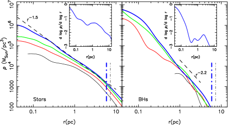
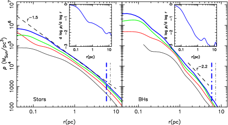
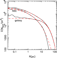
Figure 11.— Density profile of the NC in simulations B (upper panel) and C (lower panel) during the globular cluster inspirals. Left panels give the density of the NC (i.e., only particles that were initially associated with the clusters are used) after 3, 6, 9 and 12 infall events (from bottom to top), while the middle panels show the corresponding density distribution of BHs. Dot-dashed curves give the radius containing a mass in stars twice the mass of the central MBH for the initial model (black-dot-dashed curve), and for the simulation end-products (blue-dot-dashed curve). Insert panels show the radial dependence of the density profile slope $d\log\rho/d\log r$ in the final NC models. Right panels display the projected density profile of the stars in the NC, in the galaxy (i.e., only particles that were initially associated with the galaxy) and the sum of them (upper curves). Dashed-red curves are the best fitting Sérsic profile models to these projected distributions.

Figure 12.— Total mass of BHs accumulated inside the inner parsec during the inspiral simulations B (lower points) and C (upper points), as a function of the mass of the NC (i.e., the sum of the decayed globular cluster masses). The solid curves give the best fitting power law profiles to the data for $M_{\rm NC}>4\times 10^{6}M_{\odot}$. Masses are in units of solar masses.

5.2. Consecutive inspirals

In order to determine the distribution of stars and stellar remnants predicted by a dissipationless formation model for the Milky Way NC we performed simulations which followed the repeated merger of mass-segregated massive clusters in the GC; these correspond to simulations B and C of Table 1. In these integrations the number of $N$-body particles was much reduced with respect to the single inspiral simulations presented in Section 5.1. The subsampling was a necessary compromise to keep the computational time from becoming excessively long, while still allowing the simulations to follow the successive inspiral of 12 clusters into the center of the galaxy, giving a total accumulated mass in stars of $\approx 10^{7}~{}M_{\odot}$, which is roughly the observed mass of the Milky Way NC.

The process of NC formation is illustrated in Figure 11 which shows the growing central density of stars and BHs during the globular cluster inspirals. As clusters merge to the center, the peak density of the model increases and a NC forms, appearing within the model inner $\approx 10~{}$pc as an excess density of stars over the background density of the galaxy. Insert panels give the radial dependence of the density profile slope of the final NC models. In the radial range $0.5~{}{\rm pc}\lesssim r\lesssim 5~{}$pc the spatial density profile of the merger product is characterized by a density of stars which rises steeply toward the center roughly as $\sim r^{-1.5}$. At smaller radii at the end of both simulations B and C the spatial density profile of stars flattens and the radial dependence becomes approximately ${\rm d}\log\rho/{\rm d}\log r\approx-1$ inside $0.3-0.5~{}$pc. The BH population exhibits a very steep density cusp ${\rm d}\log\rho/{\rm d}\log r\approx-2.2$, outside $\sim 0.5~{}$pc, and a somewhat flat profile within this radius. The merger process produces a NC which is in an state of advanced mass-segregation, with the heavy component dominating the density of stars inside a radius of roughly $0.3~{}$pc and $1~{}$pc in simulations B and C respectively. Since smaller systems have shorter relaxation times and undergo mass-segregation more quickly, the merger process effectively reduces the mass-segregation time scale of the NC compared for instance to the models discussed in Section 2.

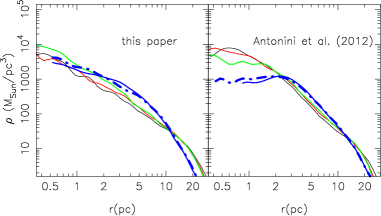
Figure 13.— Left panel shows the density profile of stars in run B after 12 inspirals were completed and that were originally part of the 3th, 6th, 9th and 12th infalling cluster. Right panel corresponds to the single mass component simulations of Antonini et al. (2012). Blue-dot-dashed curves show the density profile of stars coming from the 12th decayed cluster after the final NC model was run in isolation for a time corresponding to roughly the time that takes in our simulations for three consecutive inspiral events to complete.

The right panels of Figure 11 show the projected density of the $N-$body model at the end of the simulations. These profiles were fitted as a superposition of two model components, one intended to represent the galaxy and the other the NC. For both components we adopted the Sérsic law profile:

$$\Sigma(R)=\Sigma_{0}\text{exp}{\left[-b\left(\frac{R}{R_{0}}\right)^{\frac{1}{n}}+b\right]}~{},$$ (15)

with

$$b=2n-\frac{1}{3}+\frac{0.009876}{n}.$$ (16)

For the end product $N$-body model of run B, the best-fit parameters were $\Sigma_{0}=7.21\times 10^{3}~{}\text{M}_{\odot}/\text{pc}^{2}$, $n=1.03$, $R_{0}=31.9$ pc for the bulge, and $\Sigma_{0}=1.03\times 10^{4}~{}\text{M}_{\odot}/\text{pc}^{2}$, $n=1.88$, $R_{0}=9.51$ pc for the NC. The best-fit parameters of the merger product of run C were $\Sigma_{0}=7.44\times 10^{3}~{}\text{M}_{\odot}/\text{pc}^{2}$, $n=1.04$, $R_{0}=31.6$ pc for the bulge, and $\Sigma_{0}=7.60\times 10^{3}~{}\text{M}_{\odot}/\text{pc}^{2}$, $n=2.08$, $R_{0}=11.3$ pc for the NC.

We note that the final density profile and structure of the NC depends on a variety of factors, these include the initial distribution of stars and BHs inside the clusters, the strength of the tidal field due to the galaxy and MBH, and how the distribution of previously migrated stars and BHs evolves in response to their gravitational interaction with other background stars and with infalling clusters. For instance, the initial degree of internal evolution in the cluster models together with the adopted galactic MBH mass will determine how close to the galactic center the BH and stellar clusters will get before they completely dissociate; in turns this regulates the size of the region over which the stellar distribution flattens (i.e., the core size of the NC density profile), as well as the number of stellar BHs transported in the vicinity of the MBH.

In Figure 12 the mass in BHs accumulated in the inner parsec, $M_{\rm bh}(<1{\rm pc})$, is shown as a function of the NC mass, $M_{\rm NC}$. At any time the NC mass is given by the sum of the accumulated globular cluster masses. A good fit to the data for $M_{\rm NC}>4\times 10^{6}M_{\odot}$ is given by: $M_{\rm bh}(<1~{}{\rm pc})=a\times(M_{\rm NC}/{4\times 10^{6}M_{\odot}})^{b}$, with $a=3.33\times 10^{4}M_{\odot}$ and $b=1.44$ for Model B, and $a=1.42\times 10^{5}M_{\odot}$ and $b=0.819$ for Model C; these fitting functions are plotted in Figure 12 as solid curves.

The effect of the infalling clusters on the pre-existing NC is illustrated in the left panel of Figure 13 which shows the density profile of stars in simulation B after 12 inspirals were completed and that were originally inside the 3th, 6th, 9th and 12th infalling cluster. The density profile of stars from the 12th merged cluster, consistently with the results of the high resolution simulations of Figure 9, is characterized by a shallow density cusp out to roughly $1-2~{}$pc and an outer envelope with density that falls off rapidly with radius. The dot-dashed curve in the figure illustrates the density profile of the same stars after the final NC model was run in isolation for a time equal to the time for three consecutive inspiral events to occur, $\sim 5\times 10^{7}$yr. The similarity between the two mass distributions indicates that collisional two-body relaxation, due to random star-star and star-BH gravitational encounters, can be ignored during the inspiral simulations. The densities of stars coming from previously decayed globular clusters, however, appear very similar to each other and very different from the density of stars transported during the last inspiral, being lower and having a steeper radial dependence, ${\rm d}\log\rho/{\rm d}\log r\approx-1.5$, in the radial range $1~{}{\rm pc}\lesssim r\lesssim 10~{}$pc.

Figure 14.— Left panel: upper curves display the cumulative mass distribution of stars ($M_{\rm NC}$) in the NC at the beginning (solid curve) and at the end (dotted curve) of the 12th inspiral. The total mass in stars ($m_{\rm cl,st}$) and BHs ($m_{\rm cl,bh}$) as a function of galactocentric radius of the 12 inspiraling cluster are displayed; time increases from right to left as the cluster orbit decays toward the center and loses mass. The value of $\sqrt{M_{\rm NC}m_{\rm st}}$ is also illustrated as a function of radius; this is roughly equal to $\sqrt{M_{\bullet}m_{\rm st}}$ (double-dotted curve) at the MBH radius of influence. When the total cluster mass is larger than $\sqrt{M_{\rm NC}m_{\rm st}}$, collisional relaxation in the NC is dominated by scattering of stars and BHs from the infalling cluster. In the right panel we display the Lagrangian radii of stars from the previously decayed (11th) cluster during the 12th inspiral (dashed curves), and the evolution of the orbital radius of the 12th cluster. The orbit of the cluster is shown using a continue curve when $m_{\rm cl}>\sqrt{M_{\rm NC}m_{\rm st}}$, and a dotted curve otherwise. The evolution of the Lagrangian radii clearly shows that the inspiral modifies the mass distribution of the pre-existing NC, as argued in the text.

As illustrated in the right panel of Figure 13, this evolution was also present in the one-component inspiral simulations of Antonini et al. (2012); the initial conditions of these simulations were essentially the same as those of simulation B with the difference that the clusters only had a single mass particle group representing stars. There are two mechanisms that drive the evolution of the density profile toward their final form: (1) stars from earlier infalling clusters are stripped at smaller radii and dominate inner regions of the NC (Perets & Mastrobuono-Battisti, 2014) and, as argued in the following section, (2) gravitational scattering of the previously accumulated stars and BHs by the infalling clusters.

$\begin{array}[]{ll}\includegraphics[width=151.76964pt,angle={0}]{Figure15.ps}\end{array}$

Figure 15.— Evolution of the density profile of stars and BHs during the post-merger simulation of model B at $t=(0.09,~{}{\color[rgb]{1,0,0}0.18},~{}{\color[rgb]{0,1,0}0.27},~{}{\color[rgb]{0,0,1}0.36})\times T_{r_{\rm infl}}$. Insert panels give the radial dependence of the density profile slope $d\log\rho/d\log r$ of the final model ($t=0.36~{}{\rm T_{r_{\rm infl}}}$).

5.3. Accelerated cusp regrowth due to scattering from infalling clusters

Consider a massive cluster of mass $m_{\rm cl}$ which moves into a system of $N$ stars. The second order diffusion coefficients that appear in the Fokker-Plank equation, and which describe the evolution of the stellar distribution due to self-scattering ($\mathcal{D}_{EE,11}$) and scattering off of the cluster ($\mathcal{D}_{EE,1~{}{\rm cl}}$), scale with the mass of the perturber, the mass ($m$) and density of field particles as:

$$\mathcal{D}_{EE,11}\simeq m^{2}N;~{}~{}\mathcal{D}_{EE,1~{}{\rm cl}}\simeq m_{\rm cl}^{2},$$ (17)

where here we have approximated the cluster as a point mass perturber. From Equation (17) we see that if $m_{\rm cl}\gg\sqrt{m^{2}N}$, $\mathcal{D}_{EE,1~{}{\rm cl}}\gg\mathcal{D}_{EE,11}$, i.e., self-scattering is negligible compared with scattering off of the massive perturber; the first order coefficients can also be ignored since they are smaller than $\mathcal{D}_{EE,1~{}{\rm cl}}$ by factors of $m^{2}N/m_{\rm cl}^{2}$ and $m/m_{\rm cl}$. Thus, if

$$m_{\rm cl}>\sqrt{m^{2}N}$$ (18)

an inspiraling cluster will reduce the energy relaxation time scale compared to that due to stars alone by a factor $\sim m_{\rm cl}^{2}\ln\Lambda/m^{2}N\ln\Lambda^{\prime}$. In the latter expression, $\Lambda^{\prime}$ represents the Coulomb logarithm estimated by taking into account the large physical size of the cluster, which implies a lower effectiveness of close gravitational scattering with respect to star-star scattering (e.g., Merritt, 2013). This latter quantity can be set to

$$\ln\Lambda^{\prime}\approx\frac{1}{2}\ln\left[1+\frac{p_{max}^{2}}{p_{0}^{2}}\right]$$ (19)

with $p_{max}$ roughly 1/4 times the linear extent of the test star’s orbit. Setting this size to $5~{}$pc, and $p_{0}$ to half of the size of the cluster, $\approx 1~{}\rm pc$, the typical relaxation time becomes:

$$T^{eff}_{r}(r)\approx\frac{0.34~{}\sigma^{3}(r)}{G^{2}\ln{\Lambda^{\prime}}\rho}\frac{M_{\bullet}}{m_{\rm cl}^{2}}=2\times 10^{7}\left(\frac{\sigma}{50{\rm kms^{-1}}}\right)^{3}$$ (20)

$$\times\left(\frac{1.6}{\ln\Lambda^{\prime}}\frac{10^{3}M_{\odot}}{\rho}\frac{M_{\rm\bullet}}{4\times 10^{6}~{}M_{\odot}}\right)\left(\frac{5\times 10^{5}~{}M_{\odot}}{m_{\rm cl}}\right)^{2}{\rm yr}$$

where in deriving this expression we have used the fact that $mN\approx M_{\bullet}$ near the sphere of influence of the MBH. For $M_{\bullet}\sim 10^{7}~{}M_{\odot}$, the infall of even a cluster of $10^{4}~{}M_{\odot}$ would largely affect the rate of collisional relaxation, provided that the cluster spends a time of order $T^{eff}_{r}$ in a region where the condition (18) is satisfied.

The left panel of Figure 14 shows the total mass of BHs and stars bound to the 12th infalling cluster in run B as a function of cluster orbital radius and compares these to $\sqrt{m^{2}N}$. The cluster spends roughly $5\times 10^{6}~{}$yr before it reaches $\sim 2~{}$pc (right panel of Figure 14) after which its mass drops below $\sqrt{M_{\bullet}m}$ and self-scattering starts to be the dominant effect driving collisional relaxation. Since the time for the cluster to reach this radius is comparable to $T^{eff}_{r}$, the inspiral of clusters is expected to have an important impact on the density distribution of the preexisting NC, in agreement with the results of our simulations. In the right panel of Figure 14 we show the evolution of the Lagrangian radii of the stars transported in the NC during the previous (11th) inspiral. During the first $10^{7}~{}$yr, the condition (18) is satisfied and the inspiral induces a rapid evolution of the NC mass distribution. Note that in a real galaxy, due to the smaller individual stellar mass, scattering from the perturber would dominate down to smaller radii than in our $N$-body model. However, in the region where the condition (18) is satisfied the relaxation time in the simulations would be roughly the same as in the real system.

Scattering of stars by the massive perturber will cause an initial density core to fill up and the distribution function to evolve toward a constant value. The result is a sharp increase in the density profile of stars, $n\sim r^{-1.5}$, inside a radius approximately equal to the radius within which the condition Equation (18) is first met. After the perturber reaches a radius, $r_{\rm crit}$, containing a total mass in stars smaller than its mass, a large density core is rapidly carved out as a consequence of ejection of stars from the center. This is the evolution that for example characterizes the mass distribution of stars during the formation and evolution of MBH binaries in galactic nuclei (see Figure 13 and 14 of Antonini & Merritt, 2012). In our simulations, however, the clusters disrupt before reaching $r_{\rm crit}$, and before the second phase of cusp disruption can initiate. Thus, the net effect of infalling clusters on the pre-existing NC distribution is that of inducing a short period of enhanced collisional relaxation, which causes the central density of stars and BHs to increase during the inspirals.

5.4. collisional evolution

During and after its formation a NC will evolve due to collisional star-star, star-BH, and BH-BH interactions which will cause its density distribution to slowly morph into the steeply rising density profile which describes the quasi-steady state solution of stars and BHs near a MBH. We study the evolution of the NC due to collisional relaxation by evolving the inspiral simulations end-product of simulation B for roughly half a relaxation time (or one Hubble time when scaling the $N$-body model to the Milky Way). In order to efficiently evolve the system for such a long timescale the $N$-body model was resampled to contain a smaller number of particles. Since we are interested in the model distribution at small radii we kept the mass of the particles the same as in the original model, so that the resolution of the simulation in the region near the center was unchanged, and we included only particles with orbital periapsis less than $10$pc and apoapsis less than $20$pc. In this way the total gravitational force acting on particles lying inside $\approx 10$pc was approximately unchanged with respect to the original model. This sampling procedure is equivalent of truncating the mass distribution of the model smoothly at $r\gtrsim 10$pc. $N$-body integrations over a few crossing times verified the (collisionless) quasi-equilibrium state of the truncated model.

Since the dynamical friction times for globular clusters at $20~{}$pc from the galactic center are much shorter than relaxation times, both cluster and galaxy will not undergo a significant amount of collisional relaxation during the inspirals. In our $N$-body simulations B and C the inspiral time of the globulars to reach the center and disperse around the central MBH is about $100$ times shorter than the relaxation time of the NC. Thus, during the inspiral simulations, relaxation due to star-star, star-BH, and BH-BH interactions was ignored, while in the post-merger simulations presented here times were scaled to the relaxation time computed at the sphere of influence of the MBH. Note that for the sake of simplicity the evolution was broken into two successive stages: infall of the clusters; then evolution, due to two-body encounters, of the stellar distribution around the MBH with infalls “turned off.” In reality, subsequent inspirals would be separated by times of order a Gyr and significant two-body relaxation would occur between these events.

Figure 15 shows the evolution of the mass density in each species in the post-merger integrations. Initially, the density of BHs dominates over the density in stars at $r\lesssim 0.1r_{\rm infl}$. Thus, at radii smaller than these, the evolution of the BHs is mostly driven by BH-BH self-scattering which causes their distribution to reach, in roughly $0.2\times T_{r_{\rm infl}}$, a quasi-steady state form characterized by a steep density slope, $\gamma\approx 2.2$, at all radii. At radii larger than $\sim 0.1r_{\rm infl}$ the stars dominate the mass density and the BH population evolves due to dynamical friction against the lighter component. The general trend is for the central mass density of BHs to steadily increase with time.

While the BHs segregate to the center, the lighter particle mass density decreases within the radial range $0.1\lesssim r\lesssim 10~{}$pc. The evolution of the stellar distribution toward lower densities is a consequence of their gravitational interaction with the BHs: when the density in the BHs approaches locally the density in stars, heating of the light particles off the heavy particles dominates over star-star scattering, causing the density of the former to decrease. Scattering of stars off the BHs is also expected to promptly modify the star density profile at small radii causing the formation of a “mini-cusp” at $r\lesssim 0.02r_{\rm infl}$ (Gualandris & Merritt, 2012). We find evidence of this phenomenon in our $N$-body models which rapidily develop a $n\sim r^{-1.5}$ cusp at $r<0.03~{}$pc (see upper panel and corresponding insert panel of Figure 15). Outside these radii however, even after about half a relaxation time the star distribution retains the shallow density profile at $r\lesssim 0.2~{}$pc that characterized the initial model. We conclude that even after a time of order the relaxation time, model B looks different from the dynamically relaxed models that are often assumed to describe the density distribution of stars and BHs near the center of galaxies. After $\approx 0.4\times T_{r_{\rm infl}}$ the BHs (stars) attain a central density cusp which is steeper (shallower) than in those models.

We note that the details of the final density distribution of our NC model depends on a number of factors that remain quite uncertain. For example, the final state of the BH population in the NC and the degree at which the BHs are segregated in the final model will depend on their initial number fraction and in turns on the assumptions made for their initial distribution in the parent clusters.

$\begin{array}[]{ll}\includegraphics[width=148.29596pt,angle={270}]{Figure16a.ps}\\ \includegraphics[width=147.4292pt,angle={270}]{Figure16b.ps}\end{array}$

Figure 16.— Radial profile of the anisotropy parameter ($\beta$) and radial ($\sigma_{r}$) and tangential ($\sigma_{t}$) components of the one-dimensional velocity dispersion ($\sigma$). Plots were obtained at the end of the 12th inspiral event using only $N-$body particles that were originally inside the clusters. The blue-dashed curves in the upper panels display the anisotropy profile of the NC in simulation B at the end of the post merger phase.

5.5. Kinematics and morphology

Understanding the kinematical structure and shape of galactic nuclei is important for placing constraints on their formation history and evolution. We quantified the velocity anisotropy of our models by using the parameter:

$$\beta=1-\frac{\sigma_{t}^{2}}{2\sigma_{r}^{2}}~{},$$ (21)

with $\sigma_{r}$ and $\sigma_{t}$ the radial and tangential velocity dispersions respectively. Figure 16 shows the radial profile of $\beta$, $\sigma_{r}$ and $\sigma_{t}$ for the stellar and BH populations in simulations B and C. At the end of the inspiral simulations, model B is characterized by an approximately flat velocity anisotropy profile with $\beta\approx-0.5$ while in model C, $\beta$ slightly decreases from nearly $0$ to $-0.2$ within $1~{}$pc and it is approximately constant outside this radius. Thus, our models are tangentially anisotropic throughout $100~{}$pc, both in the stellar and BH components. The upper panels of Figure 16 also display the radial profile of the anisotropy parameter of model B at the end of the post merger phase, i.e., after the system was run in isolation for a time of order the relaxation time. Evidently, two-body relaxation causes $\beta$ to increase and the NC to evolve toward spherical symmetry in velocity space.

$\begin{array}[]{ll}\\ \includegraphics[width=173.44534pt,angle={270}]{Figure17.ps}\end{array}$

Figure 17.— Triaxiality parameter (upper panel) and axis ratios (lower panel) as functions of radius, for model B at the end of the inspiral phase (black-solid curves) and at the end of the post-merger collisional evolution (blue-dotted curves). Left panels give the shape parameters obtained by including all particles (stars and BHs) in the evaluation of the symmetry axes; in the right panels only particles representing stars that were transported to the center by the infalling stellar clusters were used.

We measured the model shape in our simulations from the moment-of-inertia tensor (e.g., Katz, 1991; Poon & Merritt, 2004; Antonini et al., 2009). The symmetry axes are calculated as

$$\tau_{1}=\sqrt{I_{11}/I_{max}}~{},~{}\tau_{2}=\sqrt{I_{22}/I_{max}}~{},~{}\tau_{3}=\sqrt{I_{33}/I_{max}}~{},$$ (22)

where $I_{ii}$ are the principal moments of the inertia tensor and $I_{\mathrm{max}}={\rm max}\{I_{11},I_{22},I_{33}\}$; particles are then enclosed within the ellipsoid $x^{2}/{\tau_{1}}^{2}+y^{2}/{\tau_{2}}^{2}+z^{2}/{\tau_{3}}^{2}=r^{2}$. These previous steps were iterated until the values of the axial ratios had a percentage change of less than $10^{-2}$. We also define a triaxiality parameter: $T\equiv\left(a^{2}-b^{2}\right)/\left(a^{2}-c^{2}\right)$. The value $T=0.5$ corresponds to the ‘maximally triaxiality’ case, while oblate and prolate shapes correspond to $T=0$ and $1$, respectively.

Figure 17 displays radial profile of the axis ratios and triaxility parameter of the model in simulation B at the end of the inspiral simulation (black-solid curves) and at the end of the post-infall evolution (blue-dotted curves). We also evaluated the shape of the NC component by only including the stars that were transported to the center from the infalling stellar clusters (right panels); the NC component appears strongly triaxial-like within 5pc and mildly triaxial (quasi-oblate) outside this radius. The formed NCs in simulations C and B shared a similar morphological structure, so we only displayed results for model B. The model morphology within $\sim 30$pc is initially mildly triaxial and evolves due to gravitational encounters toward a more quasi-spherical shape. It is important that at the end of the post-merger phase the model still exhibits a significant degree of triaxiality, $0.1\lesssim T\lesssim 0.3$. In fact, such level of asymmetry might be large enough to significantly increase the number of tidal captures of stars and stellar binaries when compared to the same rate obtained in collisionally resupplied loss cone theories where spherical geometry is often assumed both in configuration and velocity space (Merritt & Vasiliev, 2011).

6. Discussion

6.1. Comparing to the properties of the Galactic Nuclear Cluster

Star counts using adaptive optics spectroscopy and medium-band imaging have shown that the red giants at the Galctic center, the only old stars that can be resolved in these regions, have a flat projected surface density profile close to Sgr A* (Buchholz et al., 2009; Do et al., 2009). The core in the red giant population extends out to approximately $0.3-0.5~{}$pc from the center. However, due to the effect of projection, it is difficult to constrain core size and three-dimensional spatial density profile, which could be slowly rising but even declining toward the center.

It is possible that a cusp in the lower mass stars is present and that the observed core is the result of a luminosity function that changes within $0.5~{}$pc. This could be due to physical collisions before or during the giant phase (Bailey & Davies, 1999; Dale et al., 2009); or tidal interactions between stars and the central MBH (Davies & King, 2005) – mass removal can make the luminosity that a star would otherwise reach at the tip of the red-giant phase considerably fainter and prevent these objects from evolving to become observable. While these models are possible they seem not to fully explain the observations (Dale et al., 2009). Thus, it is important to consider the possibility that the red giants are indeed representative of the unresolved low-mass main-sequence stars, and that the the density core is a consequence of the NC formation history combined to a long nuclear relaxation timescale (Section 2). On this basis we can directly compare the predictions of theoretical models to the kinematics and mass distribution inferred from observations of the giant stars at the GC and draw conclusions about possible formation mechanisms for the Milky Way NC.

6.1.1 Mass distribution

Figure 11 shows that the merger of about $10~{}$clusters results into a compact nucleus with a stellar density profile that declines as $n\sim r^{-1.5}$ outside $\sim 0.5~{}$pc and flattens to $n\sim r^{-1}$ within this radius. More precisely, we consider two definitions of the core radius: (1) the projected radius, $r_{c}$, at which the surface density falls to one-half its central value; (2) the break radius, $r_{b}$, at which the density profile transits from the inner law ($n\sim r^{-1}$) to the outer density law ($n\sim r^{-1.5}$). We find $r_{c}=0.51$pc and $r_{b}=0.48$pc for Model B, and $r_{c}=0.61$pc and $r_{b}=0.59$pc for Model C. Collisional relaxation occurring during the post merger simulation of Model B reduces the size of the core with time, while inner and outer density slopes remain roughly unchanged. At the end of the simulation, after $\sim 0.3T_{\rm r_{\rm infl}}$, we find $r_{c}=0.32$pc and $r_{b}=0.18$pc. The size of the region where the density transits to a shallow profile in our models appears to be comparable to the extent of the core inferred from number counts of the red giant stars at the GC. The exact extent of the core region (and how far our models are from their steady state) is determined by a number of factors that depends on the assumptions made in the $N-$body initial conditions. For example, the size of the density core could be made larger or smaller depending on the initial degree of cluster evolution and the number fraction of BHs. However, we note that the presence of a core in the final density distribution seems to be a quite robust outcome of a merger model for NCs. For example, the single mass component simulations of Antonini et al. (2012) also produced a final NC model with a core of size $\sim 1$pc, somewhat similar to what we find in this paper. The absence of a Bahcall-Wolf cusp is naturally explained in these models, without the need for fine-tuning or unrealistic initial conditions.

Our simulations result in a final density profile having nearly the same power-law index beyond $0.5$pc as observed ($\Sigma(R)~{}R^{-1}$, Haller et al., 1996). The slope index in the inner $\sim 0.5~{}$pc of our model, $\gamma\sim 1$, is also consistent with what obtained from the surface brightness distribution of stellar light within the inner $1^{\prime\prime}$ of Sgr A* (Yusef-Zadeh et al., 2012), but appears only marginally consistent with what inferred from number counts of the red giant stars. Slope indexes in the range  $-3\lesssim\gamma\lesssim 0.8$ are consistent with what derived from observations of the giants, although negative or nearly-zero values, corresponding to centrally-decreasing or flat densities respectively, are preferred (Merritt, 2010; Do et al., 2013).

6.1.2 Kinematics

The radial profile of the velocity anisotropy of the NC could potentially provide useful constraint on its formation. Kinematic modeling of proper motion data derived from the dominant old population of giants, reveals a nearly spherical central cluster exhibiting slow, approximately solid-body rotation, of amplitude $1.4~{}{\rm kms^{-1}arcsec^{-1}}$ (Trippe et al., 2008; Schödel et al., 2009). Kinematically, the central cluster appears isotropic, with a mildly radial anisotropy at $r\lesssim 0.1~{}$pc and slightly tangentially anisotropic for $0.1~{}{\rm pc}\lesssim r\lesssim~{}1~{}{\rm pc}$; In the radial range $1^{\prime\prime}-10^{\prime\prime}$, the late-type stars are observed to have a mean projected anisotropy of $\langle 1-{\sigma_{T}^{2}/\sigma_{R}^{2}\rangle=-0.12^{+0.098}_{-1.05}}$ (Schödel et al., 2009). Do et al. (2013) found $\beta=0.01^{+0.35}_{-0.34}$ within $0.5~{}$pc.

Our models are characterized a generally flat anisotropy profile with $\beta\approx-0.5$ at the end of the inspiral simulations and $\beta\approx 0$ at the end of the post-merger evolution. Although such values are consistent with observations, we believe that future and better kinematic data that extend outside the inner parsec will be necessary in order to provide better constraints on this scenario.

We note that due to our assumption of no preferential direction of inspiral, the merger remnants in our simulations showed no significant net rotation. Recent observations of the NC in our Galaxy suggest instead a significant rotation on parsec scale (Schödel et al., 2014); this might be reconciled with a cluster merger origin for the Galactic NC if, for instance, the clusters were originally dragged down into the Galactic disk plane (where they experience an a greater dynamical friction force) and transported into the central region of the Galaxy where they then accumulated to form a dense nucleus which will then appear to rotate in the same sense of the Galaxy.

6.1.3 Kinematically cold sub-structures

Feldmeier et al. (2014) found indications for a substructure in the Galactic NC that is rotating approximately perpendicular to the Galactic rotation with $\sim 30~{}{\rm km~{}s^{-1}}$ at a distance of $\sim 20"$ or $0.8~{}$pc from Sgr A*. In addition they found an offset of the rotation axis from the photometric minor axis and argue that this hints to infalling clusters.

We look for kinematic substructures in our models by using the Rayleigh (dipole, Rayleigh, 1919) statistics $R^{\prime}$ defined as the length of the resultant of the unit vectors $l_{i},~{}i=1,...,N,$ where $l_{i}$ is perpendicular to the orbital plane of the $i^{th}$ particle and $N$ is the number of particles (a total of 5715 per cluster). For each merged cluster we computed $R^{\prime}$ over the entire course of the inspiral simulation. For a fully isotropic distribution we expect $R^{\prime}\sim\sqrt{N}$, while $R^{\prime}\sim N$ if the orbits are correlated.

As an example, Figure 18 gives $R(=R^{\prime}/N)$ as a function of time (scaled to the relaxation time of a Milky Way like nucleus). Initially, after a cluster reaches the center the orbits are strongly correlated and, as expected, $R\sim 1$, i.e., the stars from the infalling clusters distribute into a thin disk configuration initially. Due to two-body relaxation, and due to the perturbing effect of the later infalling clusters, $R$ decreases with time and approaches a value more consistent with isotropy. Figure 18 shows that all clusters maintain some degree of anisotropy during the entire corse of the simulation. But the orbits of the stars from the first 7 clusters are almost completely isotropic by the end of the simulation. The orbits of stars from the last four/five infalling clusters are still largely correlated after $\sim 3~{}$Gyr of evolution. A linear fit to the data ($R$ vs $t$) for the last decayed cluster gives: $R(t)=-0.11\times t/{\rm Gyr}+0.96$, so that it would take about $\sim 10$ Gyr for the stars to achieve a nearly isotropic distribution. These results are consistent with those of Mastrobuono-Battisti & Perets (2013), who found that it takes a time of order the relaxation time of the nucleus to fully randomize an initially cold disk.

Figure 18.— Evolution of the Rayleigh parameter $R=R^{\prime}/N$ that measures the degree of randomness of the orbital orientation of stars transported to the center by each of the 12 infalling clusters of model B. The hatched region shows the $90\%$ confidence bands expected for a fully random distribution of orbital orientations of 5715 stars. At the end of the 12th inspiral event significantly cold kinematic substructures are present in the NC model.

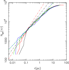
Figure 19.— Cumulative number of BHs predicted for a Milky Way nucleus as function of radius and at the different time intervals: $t=(0.09,~{}{\color[rgb]{1,0,0}0.18},~{}{\color[rgb]{0,1,0}0.27},~{}{\color[rgb]{0,0,1}0.36})\times T_{r_{\rm infl}}$, for the post-merger simulation discussed in Section 5.4. Dot-dashed curves were obtained by carrying out regression fits of $\log N_{\rm bh}$ to $\log r$ in the radial range $(r_{1},r_{2})$, with $N_{\rm bh}(<r_{1})=5$ and $N_{\rm bh}(<r_{2})=25$ (see text for details).

6.2. Extreme-mass-ratio inspirals

The inspiral of compact remnants into a MBH represents one of the most promising sources of gravitational wave radiation detectable by space-based laser interferometers (Amaro-Seoane et al., 2012). Event rates for such extreme mass-ratio inspirals are generally estimated under the assumption that the BHs had enough time to segregate and form a steep central cusp, $n\sim r^{-2}$, near the MBH. Such dynamical models predict inspiral rates per galaxies of $\sim 250~{}{\rm Gyr^{-1}}$ (Hopman & Alexander, 2006). Models that include an initial parsec scale core can result in much lower central BH densities than in the steady state models, and imply rates as low as $1-10~{}{\rm Gyr^{-1}}$ (Merritt, 2010). EMRI event rates could be also severely suppressed by the Schwarzschild barrier which limits the ability of stars to diffuse to high eccentricities onto inspiral orbits (Merritt et al., 2011).

It must be stressed that it is difficult to draw any conclusion about EMRI event rates from the models discussed in the literature because of the significant uncertainties in the underlining assumptions. Our simulations cast further doubts on results obtained from idealized time-dependent models which relay on the assumption that BHs and stars have initially the same spatial distribution. For example, based on the models discussed in Section 2 and in Merritt (2010) and Antonini & Merritt (2012), the presence of a core in the old population of stars at the GC would imply very low central densities of BHs and EMRI event rates. However, the initial conditions adopted in the simulation of Section 2 were quite artificial and not motivated by any specific physical model. We have shown that in a merger model for the formation of NCs, the resulting distribution of stellar remnants partially reflects their distribution in their parent clusters just before they reach the center of the galaxy. Thus, different, possibly more realistic, initial conditions would produce rather different central BH densities; in these models EMRI rates could be as large as (or higher than) those obtained in the steady state models even in the presence of a core in the stellar distribution.

In order to determine the number of BHs in a Milky Way like nucleus predicted by the inspiral simulations we used the scaling relation given by Equation (13). We are interested in the number of compact remnants inside $\approx 0.01$ pc, as these are the only BHs that can generate EMRIs. Since at these radii the number of BH particles in the $N-$body model is small, we carried out regression fits of $\log N_{\rm bh}$ to $\log r$ at larger radii, and extrapolate inward in order to get $N_{\rm bh}$ at the radii of interest. Following Gualandris & Merritt (2012), we performed these fits in the radial interval $(r_{1},r_{2})$ such that $N_{\rm bh}(<r_{1})=5$ and $N_{\rm bh}(<r_{2})=25$, and assume a density profile of constant power-law index. In Figure 19 we show the (scaled) cumulative number of BHs during the post merger simulations of Section 5.4. We find $N_{\rm bh}(<0.01{\rm pc})\approx 200$ at $t=0.1\times T_{r_{\rm infl}}$ and $N_{\rm bh}(<0.01{\rm pc})\approx 400$ at $t=0.3\times T_{r_{\rm infl}}$. We can directly compare the numbers so obtained with estimates from quasi-steady state Fokker Plank models of the GC. In their models, Hopman & Alexander (2006) assumed $f=0.01$, and found $N_{\rm bh}(r<0.01{\rm pc})=150$; Freitag et al. (2006) found similar values. This is similar to the number of BHs in our model at the end of the inspiral simulations but somewhat smaller than the predicted number of BHs at the end of the post merger simulations.

$\begin{array}[]{ll}\includegraphics[width=190.79385pt,angle={0}]{Figure20.ps}\end{array}$

Figure 20.— Eccentricity evolution of test particles taking different numbers of $10M_{\odot}$ perturbers: $N_{0.1}$=100, 500, 1000. The initial values of the orbital elements were: a=10 mpc, e=0.95, $\Omega=0$, $\omega=-\pi/2$ and $i=0.35\pi$. The diffusion timescale to evolve to higher angular momenta, where resonant relaxation becomes more efficient in randomizing orbital eccentricities, decreases the larger the number of BHs in the cusp.

In conclusion, a core in the density distribution of stars does not necessarily imply a low density of stellar remnants in the GC. In a merger model for NCs, BHs have a smaller core initially – as a relic of their pre-merger mass segregation, which was not fully erased by the tidal disruption process of the cluster. After a small fraction of the relaxation time ($\sim 0.1T_{\rm r_{\rm infl}}$), the BHs dynamically relax due to BH-BH interactions and attain a steep central density cusp, while the core in the stellar distribution persists. After this time, the number of BHs inside $0.01~{}$pc, the radii relevant for EMRIs, is $N_{\rm bh}(<0.01{\rm pc})\sim 100$, a value comparable to that inferred in steady state models.

$\begin{array}[]{ll}\includegraphics[width=143.09538pt,angle={0}]{Figure21a.ps}\\ \includegraphics[width=143.09538pt,angle={0}]{Figure21b.ps}\end{array}$

Figure 21.— Cumulative eccentricity distributions at $5\times 10^{7}$yr and at $10^{8}$yr of evolution for various values of the number of $10~{}M_{\odot}$ BH perutbers inside $0.1$pc, $N_{0.1}$. The insert panels give the $p$-value of the K-S tests as a function of $N_{0.1}$. Only when $N_{0.1}\gtrsim 1000$ the eccentricity distribution appears to approach a form that is consistent with observations ($p-{\rm value}\gtrsim 0.1$) after $\sim 100~{}$Myr of evolution (the S-star lifespan).

6.3. Constraining the number of dark remnants at the GC using the S-star orbits

Observations of the Galctic center have revealed the existence of $\sim 20$ young (B-type) stars orbiting within $\sim 0.05$ pc of the central black hole, the S-stars (Ghez et al., 2008; Gillessen, 2009). The S-stars are thought not to have formed in situ where the strong tidal field of the MBH would prevent star formation (Morris, 1993). Mechanisms that invoke the formation of the S-stars farther from the MBH, and subsequent rapid migration to their current location are often invoked in order to explain their existence. The current paradigm is that the S-stars result from the capture of individual stars by the tidal disruption of binaries following a close encounter to the central black hole (Hills, 1998). This formation model can successfully accounts for the number of observed S-stars (Perets et al., 2007), but it results into an orbital distribution which is largely biased toward high eccentricities, and therefore it is inconsistent with the quasi-thermal eccentricity distribution of the S-star orbits (e.g., Antonini et al., 2010). Post-migration dynamical evolution due to gravitational perturbations from a field population of BHs has been invoked in order to bring the predicted orbital distributions more in line with observations (Perets et al., 2009; Madigan et al., 2011; Hamers et al., 2014). It has been recently shown that such a scenario could indeed lead to an orbital distribution which reproduces the random and eccentric character of the observed orbits (Antonini & Merritt, 2013).

The timescale over which the S-star orbits evolve and approach the observed distribution depends on the number of objects, i.e. BHs, in the stellar cusp, being the shorter the larger the number of BHs (Antonini & Merritt, 2013). Accordingly, we determine a lower limit to the number of BHs in the GC by following the dynamical evolution of the S-stars for different values of $N_{\rm bh}$, and requiring the orbits to approach the observed distribution in $\sim 100~{}$Myr, the main-sequence life time of a B-type star.

We ignore two-body relaxation since the timescale of interest ($\sim 100~{}$Myr) is short compared with two-body (non-resonant) relaxation times near the center of the Milky Way (Merritt, 2010). Following Antonini & Merritt (2013) we assume that the semi-major axis distribution, $N(a)$, is known, and it is given by the observed values of $a$. The initial orbital eccentricities were assigned randomly in the range $0.93\leq e\leq 0.99$. The orbits were initialized at random times between $0$ and $100$ Myr and followed to a final time of $100$Myr. This setup approximately reproduces the initial conditions expected in a binary disruption scenario for the formation of the S-stars (Zhang et al., 2013). For each S-star (i.e., for each value of a), 100 integrations were carried out using the same Hamiltonian model adopted in Merritt et al. (2011) and Antonini & Merritt (2013). Briefly, the Hamiltonian model accounts for the torques due to finite-$N$ asymmetries in the field-star distribution (resonant-relaxation) and 1-PN terms which result in the (Schwarzschild) precession of the argument of periastron. The direction of the torquing field was changed smoothly with time and was randomized in a time of order the precession time of the field population as described in Section VB of Merritt et al. (2011).

We consider a field population of $10~{}M_{\odot}$ BHs,which we distributed according to a power law density profile $\rho\sim r^{-2}$. The number of BHs at radii less than $r$ is

$$N_{\rm bh}(<r)=N_{0.1}\left(r/0.1~{}{\rm pc}\right),$$ (23)

where $N_{0.1}$ is the number of BHs within a radius of $0.1$pc; we take $N_{0.1}=(100,~{}250,~{}500,~{}700,~{}1000)$, and for each of these values we compared the results of our simulations to observations by performing a two-sample Kolmogorov-Smirnov (K-S) test on the eccentricity distributions.

In any of our cusp models, most orbits have orbital eccentricities that lie initially inside (i.e., at higher eccentricity than) the Schwarzschild barrier – the locus of points in the ($E,L$) plane where resonant relaxation is suppressed by fast relativistic precession of a test particle orbit (Merritt et al., 2011). As shown in Antonini & Merritt (2013), the Schwarzshild barrier behaves as a one-way permeable membrane, which is penetrable by orbits that approach it from higher eccentricities, while it is a hard barrier for orbits that approach it from above. It can be shown that the time to diffuse above the Schwarzshild barrier, towards higher angular momenta, scales approximately with the number of perturbers as $T_{d}\sim N^{-3/2}_{\rm bh}(<a)$ or as $\sim N^{-2}_{\rm bh}(<a)$ if the choice for the coherence time is the “vector” resonant relaxation time or the mass precession time respectively – i.e., the test particles diffuse faster toward larger angular momenta, above the Schwarzschild barrier, the larger the number of background perturbers (Figure 20).

Figure 21 shows the cumulative eccentricity distributions at $5\times 10^{7}$yr and at $10^{8}$yr of evolution for various values of $N_{0.1}$. As the number of BHs in the cusp increases the diffusion timescale decreases, allowing the distribution to more rapidly approach a quasi-thermal form. The insert panels give the $p$-value of the K-S tests as a function of $N_{0.1}$. Only for $N_{0.1}\gtrsim 1000$ after $\sim 100~{}$Myr the eccentricity distribution appears to have approached a form that is consistent with observations ($p-{\rm value}\gtrsim 0.1$). These results imply that in order to explain the quasi-thermal character of the S-star orbital eccentricities, the number of BHs within $\sim 0.1~{}$pc of Sgr A* has to be $\gtrsim 1000$. Interestingly, this number is in agreement with the predictions of our globular cluster merger model (Figure 15), but appears to be much larger than the number of BHs implied by the dynamical models discussed in Section (2) which, for $f_{\rm bh}=10^{-3}$, give $N_{0.1}\approx 100$ after $10~{}$Gyr of evolution.

Interestingly, a globular cluster merger model for the Milky Way NC can potentially reconcile models which require high central densities of BHs in order to explain the orbits of the S-stars, with the “missing cusp” problem of the giant star population.

7. Summary

Understanding the distribution of stellar black holes (BHs) at the center of the Galaxy is fundamental for a variety of astrophysical problems. These include the randomization of the S-star orbits, the warping of the young stellar disk, and the inspiral of BHs into MBHs – an important class of gravitational wave sources for the future space-based interferometer antenna eLISA (Amaro-Seoane et al., 2012). The efficiency of these processes is very sensitive to the number of BHs and to their density distribution near the GC. In this paper we have used $N$-body simulations to follow the evolution of BHs in models that have not yet reached a collisional steady state. Following the evolution of the BHs for timescales of order the age of the Galaxy, we made predictions about their density distribution under the two assumptions that: (1) they follow the same phase-space distributions initially as the stars; and (2) they are initially brought into the Galactic center by dynamically evolved massive clusters. Our main results are summarized below.

• We evolved models that have a parsec-scale density core, and in which the BHs have the same phase-space distribution initially as the stars. We found that the time required for the growth of a relaxed, mass segregated stellar cusp is shorter in models which contain a population of heavy remnants (e.g., Figure 2), and it is sensitive to their initial number relative to the stars.

• Over the age of the Galaxy, and for a standard IMF, scattering off the BHs has little influence on the evolution of the lighter species. The time required for the re-growth of a mass segregated stellar cusp can be longer than the Hubble time for galaxies similar to the Milky Way (e.g., Figure 3).

• In low and intermediate luminosity galaxies globular clusters can decay to the center of the galaxy through dynamical friction and form a compact NC (Figure 5). Such clusters may harbor an inner core cluster of BHs that formed and mass-segregated to the center during the cluster evolution. For sufficiently massive clusters the BH population is likely to be retained in the cluster center, and then transported to the inner regions of the galaxy. Thus, massive clusters can represent an efficient source of BHs in the central regions of galaxies.

• We used direct $N$-body simulations to follow the inspiral and merger of globular clusters in the GC. These clusters contained two stellar populations, representing starts and BHs. Both standard and top-heavy mass functions were considered. The BHs were initially segregated to the cluster center. After about 10 inspiral events the formed NC developes a density profile that falls off as $\sim r^{-1.5}$, and a shallower core-like profile, $\gamma\lesssim 1$, inside a radius $\sim 0.5$pc. These properties are similar to those observed in the Milky Way NC. We find that the initial mass-segregation is not completely erased as the clusters are disrupted by the MBH tidal field (Figure 10). As a consequence of this, in the merger end-product the BHs dominate the total mass density within a radius of approximately $0.3~{}$pc (Figure 11).

• By continuing the evolution of the model after the final inspiral event, we find that the BH population rapidly relaxes and attains a steep central density cusp, $r^{-2.2}$. By half a relaxation time, or roughly $10$ Gyr (when scaled to the Milky Way), the core that was formed in the stellar distribution shrinks to $0.1-0.2~{}$pc (Figure 15). While the density profile slope outside these radii remained nearly unchanged the densities decreased as a consequence of heating of the stars by the BHs. Gravitational encounters also caused the NC to evolve toward spherical symmetry in configuration and velocity space.

• We studied the orbital evolution of the S-stars under the assumption that they were deposited to the GC through the disruption of binary stars by the MBH. Our analysis included the joint effects of Newtonian and relativistic perturbations to the motion, including the torques due to finite-$N$ asymmetries in the field-star distribution (resonant relaxation). We evolved the S-star orbits for a time of order $10^{8}$yr adopting models for the GC characterized by different number densities of BHs. We find that in order for the S-stars to achieve a nearly thermal distribution of eccentricities during their lifetime the GC should contain $\;\hbox to0.0pt{\lower 2.5pt\hbox{$\sim$}\hss}\raise 1.5pt\hbox{$>$}\;1000$ BHs inside $0.1~{}$pc (Figure 21). We argue that this lower limit for the number of BHs at the GC is consistent with a dissipationless formation model for the origin of the Milky Way NC.

I am grateful to R. Capuzzo-Dolcetta, D. Merritt, A. Mstrobuono-Battisti for numerous discussions about the ideas presented in this paper. I thank D. Merritt and H. Perets for useful comments that helped to improve an earlier version of this manuscript.

This research was partially supported by the National Aeronautics and Space Administration under grant no. NNX13AG92G. Computations were performed on Sunnyvale computing cluster at CITA and also on the ARC supercomputer at the SciNet HPC Consortium. SciNet is funded by: the Canada Foundation for Innovation under the auspices of Compute Canada; the Government of Ontario; Ontario Research FundResearch Excellence; and the University of Toronto.

References

- Alexander (2005) Alexander, T. 2005, Phys. Rep., 419, 65
- Alexander & Hopman (2009) Alexander, T., & Hopman, C. 2009, ApJ, 697, 1861
- Amaro-Seoane et al. (2012) Amaro-Seoane, P., et al. 2012, Classical and Quantum Gravity, 29, 124016
- Amaro-Seoane & Xian (2013) Amaro-Seoane, P., and Xian, C. 2013, arXiv:1310.0458
- Antonini et al. (2009) Antonini, F., Capuzzo-Dolcetta, R., & Merritt, D., 2009, MNRAS, 399, 671
- Antonini et al. (2010) Antonini, F., Faber, J., Gualandris, A., & Merritt, D. 2010, ApJ, 713, 90
- Antonini & Merritt (2012) Antonini, F. & Merritt, D. 2012, ApJ, 745, 83
- Antonini & Merritt (2013) Antonini, F. & Merritt, D. 2013, ApJ, 763, L10
- Antonini et al. (2012) Antonini, F., Capuzzo-Dolcetta, R., Mastrobuono-Battisti, A. & Merritt, D. 2012, ApJ, 750, 111
- Antonini (2013) Antonini, F. 2013, ApJ, 763, 62
- Antonini & Perets (2012) Antonini, F. & Perets, H. 2012, ApJ, 757, 27
- Bahcall & Wolf (1976) Bahcall, J. N., & Wolf, R. A. 1976, ApJ, 209, 214
- Bailey & Davies (1999) Bailey, V. C., & Davies, M. B. 1999, MNRAS, 308, 257
- Bartko et al. (2010) Bartko et al. 2010, ApJ, 708, 834
- Banerjee & Kroupa (2011) Banerjee, S., & Kroupa, P. 2011, ApJ, 741, L12
- Banerjee et al. (2010) Banerjee, S.,Baumgardt, H., Kroupa, P. 2010, MNRAS, 402, 371
- Böker et al. (2002) Böker, Laine, S., van der Marel, R. P., Sarzi, M., Rix, H., Ho, L. C., & Shields, J. C. 2002, AJ, 123, 1389
- Brassington et al. (2010) Brassington, N. J. et al. 2010, ApJ, 725, 1805
- Buchholz et al. (2009) Buchholz, R. M., Schödel, R., & Eckart, A. 2009, A&A, 499, 483
- Carlberg & Hartwick (2014) Carlberg, R., Hartwick, F. D. A. 2014, arXiv1401.4742
- Carollo et al. (1998) Carollo, C. M., Stiavelli, & Mack, J. 1998, AJ, 116, 68
- Capuzzo-Dolcetta & Miocchi (2008) Capuzzo-Dolcetta, R., Miocchi, P., 2008, MNRAS, 388, L69
- Capuzzo-Dolcetta (1993) Capuzzo-Dolcetta, R. 1993, ApJ, 415, 616
- Casertano et al. (1987) Casertano, S., Phinney, E. S., & Villumsen, J. V., 1987, IAU Symp. 127, Structure and Dynamics of Elliptical Galaxies, ed. T. de Zeeuw (Dordrecht: Reidel), 475
- Côté et al. (2006) Côté et al. 2006 ApJS, 165, 57
- Dale et al. (2009) Dale, J. E., Davies, M. B., Church, R. P., & Freitag, M. 2009, MNRAS, 393, 1016
- Davies & King (2005) Davies, M. B., & King, A. 2005, ApJ, 624, L25
- De Lorenzi et al. (2013) De Lorenzi, F., Hartmann, M.; Debattista, V. P., Seth, A. C., & Gerhard, O. 2013, MNRAS, 429, 2974
- Do et al. (2009) Do, T., Ghez, A. M., Morris, M. R., Lu, J. R., Matthews, K., Yelda, S., & Larkin, J. 2009, ApJ, 703, 1323
- Do et al. (2013) Do, T. et al. 2013, ApJ, 779L, 6
- Dowing et al. (2010) Downing, J. M. B., Benacquista, M. J., Giersz, M., & Spurzem, R. 2010, MNRAS, 407, 1946
- Dowing et al. (2011) Downing, J. M. B., Benacquista, M. J., Giersz, M., & Spurzem, R. 2011, MNRAS, 416, 133
- Feldmeier et al. (2014) Feldmeier, A. et al. 2014 arXiv:1406.2849
- Ferrarese et al. (2006) Ferrarese, L. et al. 2006, ApJ, 644, L21
- Figer et al. (2004) Figer, D. F., Rich, R. M., Kim, S. S., Morris, M., & Serabyn, E. 2004, ApJ, 601, 319
- Freitag et al. (2006) Freitag, M., Amaro-Seoane, P., & Kalogera, V. 2006, ApJ, 649, 91
- Forbes et al. (2008) Forbes, D. A., Lasky, P., Graham, A. W., & Spitler, L. 2008, MNRAS, 389, 1924
- Gaburov et. al. (2009) Gaburov, E., Harfst, S., & Portegies Zwart, S.
- Genzel et al. (2003) Genzel, R. et al. 2003, ApJ, 594, 812
- Ghez et al. (2008) Ghez, A. M. et al., 2008, ApJ, 689, 1044
- Gillessen (2009) Gillessen, S., Eisenhauer, F., Trippe, S., Alexander, T., Genzel, R., Martins, F., Ott, T. 2009, ApJ, 692, 1075
- Genzel et al. (2010) Genzel, R., Eisenhauer, F., & Gillessen, S. 2010, Reviews of Modern Physics, 82, 3121
- Gnedin et al. (2013) Gnedin, O. Y., Ostriker, J. P., & Tremaine S. 2013, arXiv1308.0021
- Graham & Spitler (2009) Graham, A. W. & Spitler, L. R. 2009, MNRAS, 397, 2148