Ultracold Quantum Gases in Optical Lattice with Topological Defects: Its Physics and Experimental Proposal

Abstract

In this paper we give a proposal to realize optical lattices with manipulated dislocations and study the physics of ultracold quantum gas on a two-dimensional (2D) optical square lattice with dislocations. In particular, the dislocations may induce fractional topological flux on 2D Peierls optical lattice. These results pave new approach to study the quantum many-body systems on an optical lattice with controllable topological lattice-defects, including the dislocations, topological fluxes.

Introduction. — Dislocations are areas where the atoms mismatch in a perfect crystaln ; cha . There are two basic types of dislocations, the edge dislocation and the screw dislocation. Fig.1 is the illustration of the edge dislocations where the locus of defective points in the lattice lie along a line. The lattice significantly distorted in the immediate vicinity of the dislocation line. The dislocation always plays the role of impurity that destroy the strength and ductility of metals. Thus people try to control the dislocations to increase the quality of the metals.

Recently, people recognized that due to the interplay of defect topology and the topology of the original states (the topological insulators, the topological superconductors and topological orders), the dislocations will have nontrivial quantum properties. In particular, Previous works explored the effect of dislocations on the topological insulator, which induces zero energy bound states ju ; ran . Moreover, it is predicted that a Majorana fermion zero mode may be trapped around the end of a edge dislocation in px+ipy topological superconductorqi . The ends of the edge dislocations obey non-Abelian statistics, which may be applied to realize the topological quantum computation ki2 ; free ; sar . However, in condensed matter physics, the manipulation of a dislocation in a crystal is beyond timely technology.

On the other hand, in recent years, using ultracold atoms that form Bose-Einstein Condensates (BEC) or Fermi degenerate gases to make precise measurements and simulations of quantum many-body systems has become a rapidly-developing fieldBloch's review ; review . People have successfully observed the Mott insulator–superfluid transition in both bosonicgreiner and fermionicEsslinger ; Bloch2 degeneracy gases, and have demonstrated how to produceDuan and control artificial gauge field in optical lattice ai ; fl . Without considering the harmonic trap potential, the optical lattice can be regarded as a perfect crystal without lattice defects such as the vacancy, the dislocation. To realize and manipulate the topological lattice-defect in an optical lattice is an important open issue.

In this paper we will give a proposal to realize an optical lattice with manipulated dislocations and study the physics of ultracold quantum gas on a two-dimensional (2D) optical square lattice with dislocations. In particular, the dislocations may induce fractional topological flux on 2D Peierls optical lattice (see detailed discussions below). These results pave a new way to study the quantum many-body system on an optical lattice of ultracold quantum gases with controllable topological lattice-defects, including the dislocations, topological fluxes.

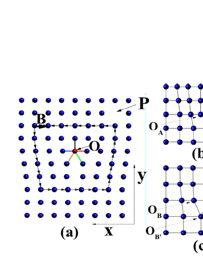
Figure 1: (Color online) (a) The illustration of the dislocation, of which the end is O site in its core denoted by a dotted circle. P site represents a vacancy that is a non-topological defect. The Burger vector $\mathbf{B}$ is also shown - the bold black arrow; (b) A-type dislocation of which the end is denoted by O_A; (b) B-type dislocation of which the end is denoted by O_B.

The Bose-Hubbard model on 2D square lattice with dislocations. — Firstly, we focus on the edge dislocations in two dimensions. The lattice with dislocation is shown in Fig.1 which can be regarded as a square lattice with an line inserted. For the lattice with dislocation along y-direction, there are five links that connect its end denoted by O (See the red spot in Fig.1(a)). To describe the topological properties of the dislocations, we define the Burger vector, $\mathbf{B}={\displaystyle\oint}d\mathbf{u}$. For the dislocation in Fig.1(a), the corresponding Burger vectors around the end O are $-\mathbf{e}_{x}$. To emphasize distinguishing features of dislocations, we also study the non-topological defect - a vacancy (the missing site denoted by P in Fig.1(a)). Fig.1(b) and Fig.1(c) show two typical edge dislocations, A-type dislocation and B-type dislocation. For a lattice of atoms in condensed matter physics, B-type dislocation is always not stable. While, in optical lattices both types of edge dislocations may exist by controlling the laser in different ways (see below discussion).

Then we consider the one-component Bose-Hubbard (BH) model on 2D square lattice with the dislocations shown in Fig.1(a), of which the Hamiltonian isfisher ; jaksch

$$H =-\sum_{\langle ij\rangle}t_{ij}b_{i}^{\dagger}b_{j}+\frac{U}{2}\sum_{i}n_{i}(n_{i}-1)$$ (1)

$$-\mu\sum_{i}n_{i}+h.c.,$$

where $b_{i}^{{\dagger}}$ and $b_{i}$ are bosonic creation and annihilation operator on site $i$. $n_{i}=b_{i}^{{\dagger}}b_{i}$ is the particle number operator on site $i$. $U$ is the strength of the repulsive interaction. Except for the lattice-site at the end of the dislocation (the red spot in Fig.1(a)), the hopping parameters $t_{ij}$ that connect the nearest neighbor sites are all set to be a positive number $t_{ij}=t$ ($i,j\neq$ O), $\left\langle i,j\right\rangle$ represents all nearest neighboring links. For the lattice-site at the end of the dislocation (the red spot in Fig.1), there are five links connecting to other lattice sites. We assume the hopping parameters on these links are $t_{ij}=t$ for the black link, $t_{ij}=t_{1}$ for the blue link, $t_{ij}=t_{2}$ for the red link, $t_{ij}=t_{3}$ for the orange link, $t_{ij}=t_{4}$ for the green link. The local properties of the BH model will dependent on the four distinct hopping parameters $t_{i}$ ($i=1,2,3,4$). In the following, we take A-type dislocation ($t_{1}=t_{2}=t$, $t_{3}=t_{4}=0$) and B-type dislocation ($t_{1}=t_{2}=t_{3}=t$, $t_{4}=0,$ or $t_{1}=t_{2}=t_{4}=t$, $t_{3}=0$) as examples to study the properties of the BH model.

This model can be solved self-consistently by the inhomogeneous mean-field (IMF) approximationfisher ; jaksch , $b_{i}^{{\dagger}}b_{j}\approx b_{i}^{{\dagger}}\langle b_{j}\rangle+\langle b_{i}^{{\dagger}}\rangle b_{j}-\langle b_{i}^{{\dagger}}\rangle\langle b_{j}\rangle,$ where $\psi_{i}=\langle b_{i}\rangle$ is the local superfluid (SF) order parameter (OP). Without translation invariance, we have one local SF OP on each lattice site that consists of the variable space of $\{\psi_{i}\}$ on all sites. $\{\psi_{i}\}$ can be solved self-consistently locally from the local Hilbert space up to $10$ one-component Bosons.

Using this IMF approach, we derive the properties of the BH model on square lattice with dislocations. For the case of strong coupling limit, $U\gg t$, the Bose gas turns into the Mott insulator (MI) phase; for the case of weak coupling limit, $U\ll t$, the ground state is the SF phase with uniform OPs, $\langle b_{i}\rangle=\psi_{i}=\psi_{0}e^{i\varphi_{0}}$ where $\psi_{0}=\left|\psi_{i}\right|=\sqrt{n_{0}}$ and $\varphi_{0}$ is an arbitrary real number from $0$ to $2\pi$.

Since we only have one dislocation, the global phase diagram remains the same as that without dislocation. In the MI phase, the SF OPs vanish, $\psi_{i}=0,$ the particle number at each site remains unit for the ground state. As a result, we find that dislocations have no significant effect in the MI phase. On the contrary, in the SF phase, we find that near the dislocations the phase factors of the local SF OPs on different sites are still uniform as Im ($\ln\frac{\psi_{i}}{\left|\psi_{i}\right|})=\varphi_{0}=$ constant; on the other hand, the amplitude of the local SF OPs and local particle density change significantly near the ends the dislocation. Near the ends of A-type dislocations O_A, the local particle density decrease; while near the ends of B-type dislocations O_B, the local particle density increase. See the illustrations in Fig.2(a) and Fig.2(b). For the SF order with B-type dislocations, the local particle density has maximum value at site O${}_{B^{\prime}}$ rather than O_B. So, the increase/decrease of local particle density near the ends of dislocations obviously comes from the increase/decrease of the connecting link numbers. That means the dislocations with different local hopping parameters show different effects on the SF order locally. The changes of local particle density $n_{i}$ near the ends of the dislocations are strongly enhanced by the on-site interaction. Fig.2(d) shows local particle density variation $\left|\Delta n/n_{0}\right|$ near the end of the dislocations via $t/U$ changes where $\Delta n=n_{i}-n_{0}$. From Fig.2(d), one can see that the on-site repulsive interaction will enhance the influence of the lattice defects on the local particle density variation.

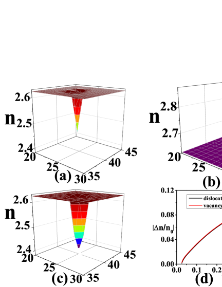
Figure 2: (Color online) (a) Particle density distribution of interacting bosons near the end (O_A site) of the A-type dislocation with $t/U=0.2$ and $\mu/U=1.5$; (b) Particle density distribution of interacting bosons near the end (O_B site) of the B-type dislocation with $t/U=0.2$ and $\mu/U=1.5$; (c) Particle density distribution of interacting bosons near the vacancy (P site) of the B-type dislocation with $t/U=0.2$ and $\mu/U=1.5$. The vacancy locates at site ($x=25$, $y=40$), on which the particle density is zero.; (d) The local particle density variation $\left|\Delta n/n_{0}\right|$ via $t/U$ on the end of A-type dislocation (O_A) and that on the nearest site adjacency to the vacancy (missing lattice site P) when $\mu/U=1.5$.

We also studied the BH model on square lattice with a vacancy (missing lattice-site P in Fig.1(a)). The results are shown in Fig.2(c). One can see that the local SF OPs and the local particle density decrease near the vacancies, that is similar to the case of A-type dislocations (see Fig.2(d)). In fact, all these lattice-defects (dislocations or vacancies) lead to small, local but observable physical consequences. In the experiments, people may detect the particle density distribution in the SF order to observe the effect from the dislocations and that from vacancies by In-situ Observationchin .

The Bose-Hubbard model on 2D Peierls lattice with dislocations. — Next, we consider the BH on 2D Peierls lattice, of which the hopping parameters $t_{ij}$ are not real numbers but have the uniform phase factors along x-direction $t_{i,i+\mathbf{e}_{x}}=te^{i\phi_{x}}$ and y-direction $t_{i,i+\mathbf{e}_{y}}=te^{i\phi_{y}}$ where $\phi_{x/y}$ is the Peierls phasepeierls1933energy When a particle moves around a plaquette, the extra phase factor of its wave-function is $e^{i\phi_{x}}\cdot e^{i\phi_{y}}\cdot e^{-i\phi_{x}}\cdot e^{-i\phi_{y}}\equiv 1$. As a result, the non-zero value of $\phi_{x/y}$ will lead to zero flux in each plaquette. See the illustration in Fig.3. So, we call this type of lattice with complex hopping parameters but no extra flux Peierls lattice. For the free bosons, the BEC occurs at finite momentum $\mathbf{k}=\mathbf{\phi}=(\phi_{x},$ $\phi_{y}).$

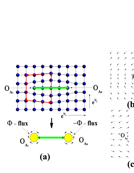
Figure 3: (Color online) (a) Illustration of the induced topological flux by A-type dislocations, $\Phi=\pm\phi_{y}$. The green line denotes the dislocation and the red lines with arrows denote the loop path to calculate the Burger vector; (b) and (c) are the IMF numerical results of the phase factors of local SF OPs of interacting bosons near the ends of A-type dislocation (O${}_{A_{L}}$ and O${}_{A_{R}}$) with $t/U=0.05,$ $\mu/U=1.5$ and $\mathbf{\phi}=(0,$ $\pi)$. It is obvious that the dislocation induces $\pm\pi$ topological flux on the Peierls lattice.

Then we study the dislocations on the Peierls lattice. An interesting property is the induced topological flux around the ends of the dislocations due to the lattice mismatch. When a Boson moves around a dislocation with the Burger vector $\mathbf{B},$ an extra phase factor will be obtained,

$$e^{i\Phi} =\left(e^{i\phi_{x}}\cdot...\cdot e^{i\phi_{x}}\right)_{N}\times\left(e^{i\phi_{y}}\cdot...\cdot e^{i\phi_{y}}\right)_{M}$$

$$\times\left(e^{-i\phi_{x}}\cdot...\cdot e^{-i\phi_{x}}\right)_{N^{\prime}}\times\left(e^{-i\phi_{y}}\cdot...\cdot e^{-i\phi_{y}}\right)_{M^{\prime}}$$

$$=\exp[i({\displaystyle\oint}\mathbf{\phi\cdot}d\mathbf{u)}].$$ (2)

A universal relationship between the induced topological flux and the dislocation’s Burger vector is given by

$$\Phi={\displaystyle\oint}d\varphi=\mathbf{\phi}\cdot\mathbf{B.}$$ (3)

Thus, the two ends of a dislocation have opposite topological fluxes, one is $\mathbf{\phi}\cdot\mathbf{B,}$ the other is $-\mathbf{\phi}\cdot\mathbf{B}$. The total induced topological flux of it is zero due to the cancelation effect.

Take the case in Fig.3(a) as an example. We have $N=4,$ $N^{\prime}=4,$ $M=4,$ $M^{\prime}=3$. As a result, we get a total phase factor $e^{i\Phi}=e^{i\phi_{y}}$. The two ends (denoted by O${}_{A_{L}}$ and O${}_{A_{R}}$) of the dislocation on the Peierls lattice play the role of a topological flux $\Phi=\pm\phi_{y}$ for all particles on the Peierls lattice.

Next, we study the properties of interacting Bosons on the Peierls lattice with dislocations by the IMF approach. From the numerical calculations, we found that the local SF OPs show nontrivial topological properties. For example, for $\mathbf{\phi}=(0,$ $\pi)$, there indeed exists an $\pm\pi$ flux around the ends of the dislocations along x-direction. From the numerical results, the phase pattern of topological vortices near the ends (O${}_{A_{L}}$ and O${}_{A_{R}}$) of the A-type dislocation Im ($\ln\frac{\psi_{i}}{\left|\psi_{i}\right|})=\varphi_{i}$ is given in Fig.3(b) and Fig.3(c). The situation is qualitatively different from the SF order with a vacancy on the Peierls lattice. In particular, the induced topological flux of the dislocations in the Peierls lattice is protected by the topological properties of the dislocations. And the fluctuations of the four distinct hopping parameters $t_{i}$ ($i=1,2,3,4$) will never change the topological flux. As a result, the induced topological flux from A-type dislocation is same to that from B-type.

Fermi degenerate gases on 2D square lattice with dislocations. — In addition, we studied the free Fermi degenerate gases on a 2D square lattice with dislocations. To observe the effect of the dislocation on the Fermi liquid, we calculate the local density of states (LDOS) of the system. The LDOS can be expressed by $N(\mathbf{r},\omega)=-\frac{2}{\pi}$Im $[$Tr $G(\mathbf{r},\mathbf{r};\omega)]$ in terms of the retarded Green’s function $G$. For the perfect lattice without dislocations, the LDOS is uniform. When there exists a dislocation, the LDOS exhibits a quantum interference pattern near the ends of a dislocations. Besides, the numerical results in Fig.4 show the significant Friedel oscillations away from the ends of a dislocationsfre . However, for the case of a vacancy, there is no such defect induced quantum interference pattern. These predictions could also be observed by In-situ Observation on the optical lattice with dislocations.

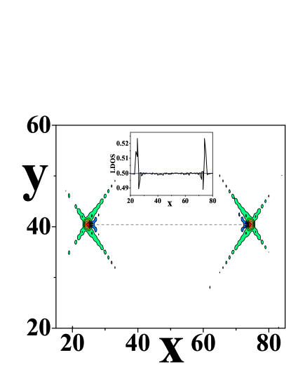
Figure 4: (Color online) The local density of states of quantum interference pattern near the ends of a dislocations for the half filling case. The system has open boundary condition. The black dotted line denotes the dislocation. x, y denote the lattice sites. The inset shows the oscillating local density of states along the dislocations ($y=40$).

However, quite different from the case of Bose gas, the induced topological flux causes little effect on the Fermi degenerate gas.

The physical realization — In the followings we discuss the physical realization of the 2D optical lattice, particularly the Peierls lattice with dislocations.

For the first step, we give a proposal to realize an optical lattice with dislocations by using the interference effect of the optical vortex wave. An optical vortex is a beam of light whose phase varies in a screw thread like manner along its axis of propagation. The optical vortex waves possess a phase singularity which occurs at a point or a line where the physical property of the wave becomes infinite or changes abruptly. We use the properties of vortices to realize the dislocations Nye J F ; sch ; Yu N .

An ideal optical vortex propagating in the $z$ direction may be written in the cylindrical coordinate as $E(r,\varphi,z)=A(r,z)e^{im\varphi}e^{-ikz},$ where $A(r,z)$ is amplitude function, $k=2\pi/\lambda$ is the wave number, and $m$ is known as the topological charge. The optical system is shown in Fig.5: a plane wave and an optical vortex wave propagate in the $xz$ plane with wavelength $\lambda_{1}$, linearly polarized in $y$ direction, and an optical standing wave in the $xy$ plane with wavelength $\lambda_{2}$, linearly polarized in $x$ direction. The optical vortex wave propagates along the $z$ axis. The plane wave in $xz$ plane is traveling in $z$ axis at an angle $\theta$ to the optical vortex wave. The intensity of light in receiving plane at $z_{0}$ can be written as:

$$I\propto\cos(k_{1}(\sin\theta x+\cos\theta z_{0}-k_{1}z_{0})+m\varphi+\phi_{0})+\cos^{2}(k_{2}y),$$ (4)

where $k_{1}=2\pi/\lambda_{1}$, $k_{2}=2\pi/\lambda_{2}$, $m$ is the topological charge, $\phi_{0}$ is the phase shift from the optical path difference between the optical vortex and the plane wave in the $xz$ plane, $\varphi=\tan^{-1}(x/y)$. We will set the interfering plane at $z_{0}=0$ in all our simulation. The results is shown in Fig.6. The simulation region is $5\times 5\mathrm{um}$. We have taken $\lambda_{1}=500\mathrm{nm}$, $\lambda_{2}=600\mathrm{nm}$ in our simulations.

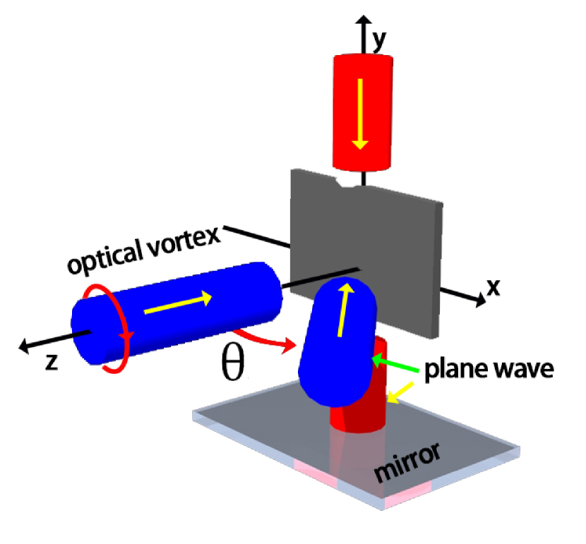
Figure 5: The experimental setup to generate an optical lattice with dislocations: a plane wave and an optical vortex wave propagate in the $xz$ plane with wavelength $\lambda_{1},$ optical standing wave propagates in the $xy$ plane with wavelength $\lambda_{2}$, linearly polarized in $x$ direction.

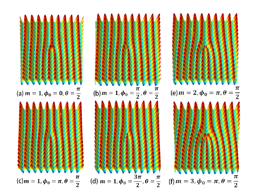
Figure 6: The intensity distributions for different dislocations with different phase shifts in optical lattice.

From Fig.6(a, b, c, d), we can see that the optical lattice around the dislocation is sensitive to the phase shift between the optical vortex and the plane wave. So we need to adjust the phase shift properly to obtain the designed dislocation optical lattice, which can be realized by tunable phase plate. The fringe spacing would increase due to the decrease of the angle $\theta$. So an A-type dislocation (Fig.6(a)) can evolute into a B-type (Fig.6(d)) one smoothly by tuning the angle $\theta$. This procedure also indicates the topology-equivalence between A-type and B-type dislocations. In addition, we can also generate a dislocation with higher Burger vector if the topological charge $|m|>1$, as shown in Fig.6(e, f).

For the second step we show how to realize the Peierls optical lattice. Recently, in experiments, tunable Peierls phases in a 1D “Zeeman lattice” have been realized using a combination of radio-frequency and Raman coupling jimenezGarcia2012peierls . Now, a hot topic is to realize the spatially-dependent Peierls phases that leads to an effective (staggered) magnetic flux through one unit cell of the optical lattice. Thus, to engineer uniform complex hopping amplitudes with Peierls phases along y-directionpeierls1933energy , $t_{i,i+\mathbf{e}_{y}}=te^{i\phi}$, the Raman-assisted hoppings are used by a pair of far-detuned running-wave laser beams with different frequencies, $\omega_{0}$ and $\omega_{0}+\Delta$Eckardt2005localization ; Lignier2007 ; Chen2011controlling ; kolovsky2011creating . A linear potential is added along y-direction, of which the energy difference between two nearest neighbor sites is $\Delta.$ So the Raman-assisted hoppings are restored along y-direction with the energy resonance $\hbar\omega=\Delta$. However, along x-direction, there is no such Raman-assisted hoppings. As a result, we can get uniform complex hopping amplitudes with Peierls phases along y-direction, $t_{i,i+\mathbf{e}_{x}}=t,$ $t_{i,i+\mathbf{e}_{y}}=te^{i\phi_{y}}$. By similar approach and tuning the directions of the two Raman laser beams, we can get different uniform complex hopping amplitudes with Peierls phases along both x-direction and y-direction.

Conclusion — In this paper we studied the physics of ultracold quantum gases on a two-dimensional (2D) optical square lattice with dislocations. We found that for the Boson’s SF order in conventional 2D square lattice, the dislocations will slightly change the local particle density and lead to small, local but observable physical consequences. In particular, the dislocations may induce fractional topological flux on 2D Peierls optical lattice from the interplay between the Peierls phases on hopping amplitudes and the nonlocal properties of the dislocations. In this case, the topological optical vortex eventually results the topological vortex of SF of Bosons in optical lattice. In the future, this realization may be applied to realized nontrivial topology in topological ordered states.

* * *

This work is supported by National Basic Research Program of China (973 Program) under the grant No. 2011CB921803, 2012CB921704 and NSFC Grant No. 11174035 and 11374037.

References

- (1) D. R. Nelson, Defects and Geometry in Condensed Matter Physics, (Cambridge University Press, 2002).
- (2) P. M. Chaikin and T. C. Lubensky, Principles of Condensed Matter Physics, (Cambridge university press, 1995).
- (3) Y. Ran, et.al, Nature Phys. 5, 298 (2009).
- (4) V. Juricic, et.al, Phys. Rev. Lett. 108, 106403 (2012).
- (5) T. L. Hughes, et.al, arXiv:1303.1539.
- (6) A. Kitaev, Ann. Phys. 321, 2-111 (2006).
- (7) M. Freedman, et.al, Math. Phys. 227, 605-622 (2002).
- (8) C. Nayak, et.al, Rev. Mod. Phys. 80, 1083-1159 (2008).
- (9) I. Bloch, et.al, Rev. Mod. Phys. 80, 885 (2008).
- (10) S. Giorgini, et.al, Rev. Mod. Phys. 80, 1215 (2008).
- (11) M. Greiner, et al., Nature 415, 39 (2002).
- (12) R. Jödens et al., Nature (London) 455, 204 (2008).
- (13) U. Schneider et al., Science 322, 1520 (2008).
- (14) L.-M. Duan, et al., Phys. Rev. Lett. 91, 090402 (2003).
- (15) J. J. Garía-Ripoll, et al., Phys. Rev. Lett. 93, 250405 (2004).
- (16) S. Trotzky et al., Science 319, 295 (2008).
- (17) M. Aidelsburger, et al, Phys. Rev. Lett. 107, 255301 (2011); M. Aidelsburger, et al, Phys. Rev. Lett. 111, 185301 (2013).
- (18) H. Miyake, et al, Phys. Rev. Lett. 111, 185302 (2013).
- (19) M. P. A. Fisher, et al., Phys. Rev. B 40, 546 (1989). 045305(2012).
- (20) D. Jaksch, et al., Phys. Rev. Lett. 81, 3108 (1998).
- (21) N. Gemelke, et al., Nature 460, 995-998 (2009).
- (22) R. E. Peierls, Z. Phys. 80, 763 (1933).
- (23) J. Friedel, Adv. Phys. 3, 446 (1954).
- (24) A. Eckardt, et.al, Phys. Rev. Lett. 95, 200401 (2005); A. Eckardt, and M. Holthaus, EPL. 80, 50004 (2007).
- (25) H. Lignier, et al., Phys. Rev. Lett. 99, 220403 (2007).
- (26) Y.-A. Chen, et al., Phys. Rev. Lett. 107, 210405 (2011).
- (27) A. Kolovsky, Europhys. Lett. 93, 20003 (2011).
- (28) K. Jiménez-García, et al., Phys. Rev. Lett. 108, 225303 (2012).
- (29) Nye J F, Berry M V, Proceedings of the Royal Society of London. A. Mathematical and Physical Sciences, 336(1605): 165 (1974).
- (30) E. Schonbrun, R. Piestun, Optical Engineering 45, 028001 (2006)
- (31) Yu N, Genevet P, Kats M A, et al, Science, 334(6054): 333 (2011).