Mass-Radius Relations and Core-Envelope Decompositions of Super-Earths and Sub-Neptunes

Abstract

Many exoplanets have been discovered with radii of 1$-$4 R_⊕, between that of Earth and Neptune. A number of these are known to have densities consistent with solid compositions, while others are “sub-Neptunes” likely to have significant H₂-He envelopes. Future surveys will no doubt significantly expand these populations. In order to understand how the measured masses and radii of such planets can inform their structures and compositions, we construct models both for solid layered planets and for planets with solid cores and gaseous envelopes, exploring a range of core masses, H₂-He envelope masses, and associated envelope entropies. For planets in the super-Earth/sub-Neptune regime for which both radius and mass are measured, we estimate how each is partitioned into a solid core and gaseous envelope, associating a specific core mass and envelope mass with a given exoplanet. We perform this decomposition for both “Earth-like” rock-iron cores and pure ice cores, and find that the necessary gaseous envelope masses for this important sub-class of exoplanets must range very widely from zero to many Earth masses, even for a given core mass. This result bears importantly on exoplanet formation and envelope evaporation processes.

1. Introduction

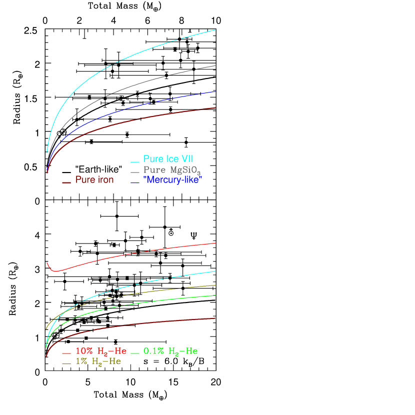
Figure 1.— Comparison of known exoplanets and Solar System planets with our models of simple Fe core/MgSiO₃ mantle planets, pure water (Ice VII) planets, and planets with H₂-He envelopes. Earth-like is defined as 32.5% core mass fraction (CMF) and Mercury-like is defined as 70% CMF (2007ApJ...669.1279S). The range of possible mass/radius values for several planets lie squarely within the area occupied by Fe core/MgSiO₃ mantle planets, making them excellent terrestrial exoplanet candidates. A number of others lie between the pure MgSiO₃ and pure Ice VII curves, making them, perhaps, candidates for “water worlds,” or for possessing small H₂-He envelopes. Another population of planets at a wide range of masses is consistent only with deeper H₂-He envelopes. The measured mass and radius values and references for the plotted planets are given in Table 2.

The detection of thousands of candidate exoplanets with a wide range of masses and radii motivates the study of the general structure of planetary bodies. While early detection methods heavily favored large planets with masses and radii near those of Jupiter, the recent trend has been toward lower masses and radii, some of which appear to be terrestrial, e.g. Kepler-10b, which was recently confirmed as a planet with radius $1.416^{+0.033}_{-0.036}R_{\earth}$, mass $4.56^{+1.17}_{-1.29}M_{\earth}$, and average density $8.8^{+2.1}_{-2.9}$ g cm^-3 (2011ApJ...729...27B). For comparison, the average densities of the Earth and Venus are $5.5$ g cm^-3 and $5.2$ g cm^-3, respectively.

2013arXiv1311.0329L have suggested that it is likely that planets larger than about 1.75 R_⊕ (based on mass-radius relations) have hydrogen/helium envelopes that contribute significantly to their radii. In particular, they find that a planet’s radius alone provides a first-order estimate of its composition, specifically, the H₂-He mass fraction. There is some uncertainty in this limit. For example, 2014ApJ...783L...6W adopt a maximum solid planet radius of 1.5 R_⊕, based in a maximum in the density distribution at $\sim$1.5 R_⊕ and $\sim$7.6 M_⊕ and Marcy.in.press interpret this as a transition radius of 2.0 R_⊕, given an observed decrease in density from 1.5 to 2.0 R_⊕.

Similarly, 2011ApJ...727...86R suggests that envelope accretion onto a core, leading to a significant gaseous envelope, begins at a core mass of 10 M_⊕, or perhaps larger if the planets form close to their stars. However, recent observations of known exoplanets suggest that envelope accretion begins, on average, at a lower mass (as found by 2014ApJ...783L...6W), and some individual planets appear to acquire gaseous envelopes at very low masses. For example, Kepler-51b has been measured to have a mass of $2.1_{-0.8}^{+1.5}$ M_⊕ and a radius of $7.1\pm 0.3$ R_⊕, corresponding to a density of 0.03${}^{+0.02}_{-0.01}$ g cm^-3 (2014arXiv1401.2885M), clearly indicating a mostly gaseous composition.

Recent space-based missions such as Kepler (2010Sci...327..977B) and CoRoT (2006ESASP1306...33B) had photometric precision capable of measuring transits by Earth-sized planets. In the first 16 months of the Kepler Mission, 207 Earth-sized ($R_{p}<1.25R_{\earth}$) and 680 super-Earth-sized ($1.25R_{\earth}<R_{p}<2R_{\earth}$) planetary candidates were reported (2013ApJS..204...24B), suggesting a large number of solid planet candidates given a $\sim$1.75 R_⊕ cutoff. Figure 1 provides a comparison of planets with measured radii and masses with theoretical mass-radius curves that we have generated for various simple planet compositions, including pure iron, Earth-like, Mercury-like, and pure silicate. We also include on Figure 1 a pure water$-$in the form of Ice VII$-$mass-radius curve and three curves for models with gaseous envelopes: an “Earth-like” solid core and H₂-He mass fractions of 0.1%, 1%, and 10%.

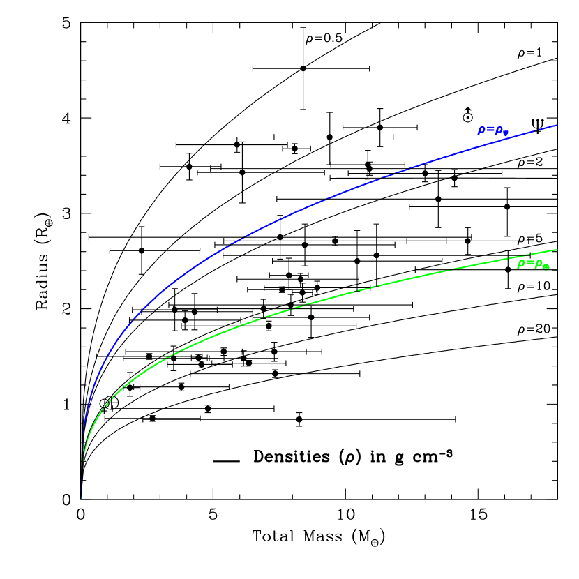
Figure 2.— Known extrasolar planets plotted against constant density curves, including Earth’s density (green) and Neptune’s density (blue). Densities ($\rho$) are given in g cm^-3.

As Figure 1 demonstrates, the mass/radius values of several known planets are consistent with an iron/rocky composition, and consistent with an Earth-like composition in particular. On the other hand, a number of observed planets have densities between those of pure water and pure silicate and are consistent with models of both “water-worlds” with a high water content and no significant envelopes, and models with H₂-He envelopes. Based on our models, the radius of a pure water, 10-M_⊕ planet is 2.5 R_⊕, which is near an observed break in the planet occurrence function in Kepler observations (2012ApJS..201...15H; 2013ApJ...778...53D). However, it is not known which of these models (if either) is dominant in this radius range or whether this break reflects an actual difference in composition between planets smaller and larger than 2.5 R_⊕.

In Figure 1, we note a very wide spread in the mass-radius distribution for planets more massive than $\sim$2 M_⊕, with a variation of $\sim$2 R_⊕ at a given mass. For planets $\lesssim$8 M_⊕, this range overlaps with an Earth-like composition with no significant gaseous envelope. For higher-mass planets, some of these are also consistent with a no-envelope model if they have a sufficient water content, but we also observe planets with large radii that are consistent only with a structure that includes a deep H₂-He envelope, even at low masses ($\gtrsim$2 M_⊕).

In Figure 2, we plot the extrasolar planets against constant density curves. Earth-density (green) and Neptune-density (blue) curves are included. The figure shows that density can vary by a factor of $\sim$5 between individual planets with the same radius. This large scatter makes it very difficult to fit any precise trends in radius with increasing mass.

In order to determine whether a given mass/radius pair indicates a solid composition, however, solid planet models and models of planets with gaseous envelopes must be constructed and compared with the data. These exoplanets may potentially have a wide range of possible compositions and temperatures and a similarly wide range of possible gaseous envelopes, so models must be able to be adjusted accordingly. Solid exoplanet models are important in both cases, since they may be used to model solid cores of planets with gaseous envelopes by applying a non-zero-pressure boundary condition at the core-envelope interface.

While there is a rich history of exoplanet structural modeling, there are a number of important areas which have yet to be investigated. For planets with gaseous envelopes, the effects of irradiation and atmospheric heating are poorly understood, and the degeneracies of envelope mass, envelope entropy, and core mass have not been explored in detail. Moreover, the implications of the large scatter in the mass-radius distribution, particularly on the search for Earth-like planets, are only beginning to be addressed.

For solid planets, equations of state for planetary materials at the pressures found in planets are subject to a degree of uncertainty, and different EOS models produce different results, which warrant analysis of the uncertainty in the modeled mass and radius values.

Our paper investigates the uncertainties and degeneracies in exoplanet modeling, particularly of planets with H₂-He envelopes, in order to gain a better understanding of what is measurable in observed exoplanets. We compute mass-radius curves over the range of 0.1 to 20 M_⊕ for a variety of planet attributes, and explore the possibility of determining a precise core-envelope decomposition from mass and radius observations. We study planets with both “Earth-like” cores and ice cores, which may both be of interest depending on whether planets with gaseous envelopes form beyond the snow line. We also compute mass-radius curves for various compositional profiles for solid planets. Note that observations suggest that planets more massive than $\sim 4-8$ M_⊕ are likely to possess significant H₂-He envelopes (2014ApJ...783L...6W), and the same is expected to be true of planets with radii larger than 1.5$-$2.0 R_⊕ (2013arXiv1311.0329L; 2014ApJ...783L...6W; Marcy.in.press), so our results for purely solid planets likely apply only to smaller and less massive objects. Conversely, our results for planets with H₂-He envelopes will apply to planets larger than $\sim 4-8$ M_⊕ or 1.5$-$2.0 R_⊕.

While e.g. (2013arXiv1311.0329L) perform evolutionary calculations to produce planetary structural models, because of the large uncertainties in the parameters that go into these calculations, we do not do this, and we believe that they do not constitute an improvement over our method. Specifically, the ages of known exoplanets are, in most cases, not measured, so that a wide range of ages is possible. Metallicities affect opacities, which in turn affect the cooling rate. They also affect the mean molecular weight and scale height of the atomsphere. Because the formation mechanism of these planets is not known, it is not appropriate a priori to estimate their uncertainties by analogy with Uranus and Neptune. In addition, irradiation is usually treated in an ad hoc manner by averaging the stellar flux over the entire planet rather than modeling day-to-night heat redistribution, which 2010ApJ...722..871S show has a significant effect on the net cooling rate.

All of these effects will influence the outcome of an evolutionary model, resulting in large uncertainties. Therefore, we sidestep these uncertainties by focusing on a single variable, the entropy of the envelope, and compute structural models over a range of entropies. The entropy and surface gravity of a planet completely determine its structure (with a small correction for metallicity), so our models are, in effect, the same as those provided by evolutionary calculations.

Section 2 summarizes the previous work modeling solid exoplanets and sub-Neptunes. Section 3 presents our models with H₂-He envelopes and the effect on radius of varying the core mass, envelope mass, and entropy in the envelope. In Section 4, we explore the core-envelope decomposition and produce a fit to the mass-radius relation of 2014ApJ...783L...6W. Section 5 gives an overview of the quantitative effects of varying our model parameters. Section 6 demonstrates our code’s output with density-pressure profiles of planets, central pressures and densities, and envelope base pressures. Section 7 presents our models of solid planets, and Section 8 summarizes our overall conclusions. Our modeling procedure, associated code, and our studies and selection of our equations of state are described in the Appendix.

2. Previous Work on Solid Exoplanets and Sub-Neptunes

Early efforts to calculate mass-radius relationships for planetary bodies of various compositions were made by 1969ApJ...158..809Z, using a Thomas-Fermi-Dirac equation of state (TFD EOS) described in 1967PhRv..158..876S. Those authors integrated the equations of hydrostatic equilibrium in conjunction with their EOS and a zero-pressure surface boundary condition to construct planetary structural models. This is the standard procedure for solid planet modeling; most recent advances have been in the accuracy of the low-pressure EOS, driven by the availability of experimental pressure/density data (2001GeoRL..28..399A).

The TFD EOS is valid only in the high-pressure limit where electrons are a non-interacting degenerate gas, but 1967PhRv..158..876S used a correlation energy correction to account for interactions between the electrons at lower pressures. They thereby extended the validity of their EOS down to $\sim$1 Mbar (by their estimation). However, as the TFD EOS does not account for chemical structure, it has zero-pressure density errors up to a factor of 2 (1969ApJ...158..809Z). As such, 1969ApJ...158..809Z focused on high-mass planets whose internal pressures lay largely in the $\gtrsim$1 Mbar regime, calculating a “critical mass” for various compositions beyond which a planet’s radius decreases with additional mass. They investigated only simple monatomic elemental compositions (pure H, He, C, Mg, Fe, and various H/He mixtures) because these are most easily modeled by the TFD EOS, which considers each element separately (1967PhRv..158..876S). In addition, 1969ApJ...158..809Z derived the maximum radius, and the mass and central pressure at which the maximum radius is achieved, as a function of He ratio in a H₂-He planet. Their models assumed a constant composition throughout the planet with no core-mantle-envelope differentiation, which limits their applicability for solid exoplanets.

More recent work implements equations of state based on experimental data. An early example of this approach is 1982AREPS..10..257S, who used contemporary shock wave data as the basis for his low-pressure equations of state for ices (H₂O, CH₄, and NH₃). 1982AREPS..10..257S also investigated the interior structure and composition of giant planets, and produced mass-radius diagrams for various compositions. He reported a lack of accurate equations of state available for ferromagnesian rock, and as such, solid planet models were outside of the scope of his paper.

In the last decade, a number of authors have presented models of solid exoplanets, motivated by the aforementioned exoplanet detections, as well as the increased availability of valid semi-empirical models for terrestrial materials. 2006Icar..181..545V defined and modeled two exoplanet classes: “super-Earths,” with similar compositions to Earth and planet mass 1 M${}_{\earth}<M_{p}<10$ M_⊕, and “super-Mercuries,” with similar compositions to Mercury and planet mass 1 M${}_{\textrm{Mercury}}<M_{p}<10$ M${}_{\textrm{Mercury}}$. It should be noted, however, that the term “super-Earth” is now often used to refer to any “terrestrial” planet with a mass greater than that of Earth, as well as planets in the 1$-$10 M_⊕ range (2011arXiv1108.0031H), or the 1.25$-$2.0 R_⊕ range (2013ApJS..204...24B). The models of 2006Icar..181..545V, along with many other contemporary models (2007Icar..191..337S; 2007ApJ...669.1279S; 2007ApJ...659.1661F), used a fourth-order Runge-Kutta integration scheme to solve the equations of hydrostatic equilibrium. The equations of state used by 2006Icar..181..545V were zero-temperature Birch-Murnaghan (B-M) equations of state (2000ipei.book.....P) with thermal corrections using a Debye model. The B-M EOS is based on low-temperature pressure/density data. Because there are limits to the pressures that such experiments can reach, the B-M EOS incorporates an extrapolation to higher pressures. Though the thermal corrections to the equations of state for rocky materials are generally small, the model of 2006Icar..181..545V required a detailed temperature profile in order to calculate the phase transitions in the silicate mantle. Their thermal model relies on the assumption of convective heat transport in the core and mantle, with conductive layers at the core-mantle boundary and the surface. They iterated their model, using the compositional profile to determine parameters to compute the temperature profile, which was used in turn to determine phase transitions for the compositional profile calculation, until a self-consistent planet model was achieved.

Table 1Equations of State Used in Recent Super-Earth Modeling Papers

Authors	Material	EOS	References
2006Icar..181..545V	Fe; FeO; Fe+alloy; (Mg1-x, Fex)2SiO4 (olivine, wadsleyite, ringwoodite); (Mg1-x; Fex)SiO3 perovskite; (Mg1-x, Fex)O	3${}^{\textrm{rd}}$ order B-M, with Debye correction	1,2,3,4
2007ApJ...656..545V	Same as 2006Icar..181..545V, plus H2O (ice)	Vinet, with Debye correction	2,3,5,6,7,8
	H2O (liquid)	Rankine-Hugoniot	9
2007ApJ...659.1661F	H2O, olivine	ANEOS	10
	iron	SESAME 2140	11
	H2-He	1995ApJS...99..713S	12
2007Icar..191..337S	Same as 2007ApJ...656..545V (but different H2O [liquid] EOS)	3${}^{\textrm{rd}}$ order B-M	2,6,13,14, 15,16,17,18
2009ApJ...693..722G	H2O (liquid)	2${}^{\textrm{nd}}$ order B-M	19
2007ApJ...669.1279S	C (graphite); Fe ($\alpha$); FeS; H2O (ice VII); MgO; MgSiO3 (enstatite); [Mg,Fe]SiO3 (perovskite); SiC	3${}^{\textrm{rd}}$ order B-M	5,15,20,21, 22,23,24, 25,26
	Fe ($\epsilon$)	Vinet	27
	H2O (liquid)	logarithmic EOS	28
	H2O (VII$-$X transition)	tabular DFT calculations	29
	All (high pressure)	Thomas-Fermi-Dirac (TFD)	30
2011ApJ...738...59R	Same as 2006Icar..181..545V	Same as 2006Icar..181..545V	5,15,20-30
	H2-He	1995ApJS...99..713S	12

2007ApJ...656..545V applied this model to the exoplanet GJ 876d and introduced a water layer consisting of high-pressure ices covered by a thin liquid water ocean. They also used a Vinet EOS fit (1989JPCM....1.1941V), as opposed to the B-M EOS used by 2006Icar..181..545V, because the Vinet fit is reported to extrapolate better to high pressures (1996JPCM....8...67H). The model from 2006Icar..181..545V was also applied in 2007ApJ...665.1413V to investigate degeneracies in the iron core, silicate mantle, and H₂O mass fractions for a given planet mass and radius and to construct ternary diagrams showing curves of constant radius for a given mass.

2007Icar..191..337S used a similar physical approach to that of 2006Icar..181..545V, but employed the stellar composition (minus H₂ and He) of the planet in constructing structural models. This approach is justified by observations that meteorite chemical ratios (thought to be representative of early planets) are similar to those found in the Sun. They used five independent parameters to determine the composition and internal structure of the planet: Mg/Si, Fe/Si, Mg# (defined as the mole fraction Mg/(Mg + Fe) in silicates), H₂O mass fraction, and total mass. They also determined a mass-radius model for planets with a water ocean.

2007ApJ...669.1279S conducted a broader investigation of solid exoplanets by using a simpler zero-temperature model that incorporated the Thomas-Fermi-Dirac EOS at high pressures with the Vinet semi-empirical EOS at lower pressures. They did not address phase transitions in the silicate mantle because phase transitions have little effect on the mass-radius curve of a given material and require a temperature profile. Instead, they assumed a constant-composition MgSiO₃ (perovskite) mantle. These simplifications allowed them to investigate a wide range of planet compositions and masses.

2007ApJ...659.1661F took an even broader approach, investigating five orders of magnitude in mass (0.01 Earth masses to 10 Jupiter masses) and a variety of planetary compositions, as well as envelopes. For the solid components of their planets, they used a model similar to that of 2007ApJ...669.1279S, though they used Mg₂SiO₄ (olivine) for the mantle instead of MgSiO₃ (perovskite), and used tabular EOS data from the ANEOS (Thompson1990) and SESAME (LyonJohnson1992) compilations, as opposed to semi-empirical fits. They neglected thermal corrections for the Mg₂SiO₄ (olivine) and iron equations of state, but for water they used a thermal EOS correction of the form

$$P=P_{0}+3.59\times 10^{-5}\rho T,$$ (1)

where $P$ is the corrected pressure in Mbar, $P_{0}$ is the zero-temperature pressure in Mbar, $\rho$ is the density in g cm^-3, and $T$ is the temperature in Kelvin. Their main goal was to produce a general, if very approximate, theory for comparison with observational data, and as such they neglected the details found in some previous papers.

2009ApJ...693..722G extended the work of 2007Icar..191..337S to masses of 100 M_⊕ and also compared it with contemporary models to determine how precisely planetary compositions can be determined from mass and radius data, in particular, the water mass fraction. They found that, given uncertainties in internal structure, the water fraction can be determined with a standard deviation of 4.5% if the mass and radius are known exactly, but this uncertainty increases rapidly with the uncertainty in the radius.

2011ApJ...738...59R also investigated planets with significant H₂-He envelopes in the context of estimating plausible masses of Kepler planet candidates of radius 2$-$6 R_⊕. They considered planet models with up to four layers: iron, silicates, water, and a hydrogen-helium envelope. They defined the exterior boundary condition as the radius at which the radial optical depth of the atmosphere is $\tau_{R}=2/3$. They used the same EOS as 2007ApJ...669.1279S for the solid components and the tabular EOS of 1995ApJS...99..713S for the gaseous envelopes. They computed a temperature profile based on radiative transfer and radiative diffusion in the outer part of the envelope, transitioning to an adiabatic profile at the onset of convection. They considered planets produced by simulations of both core-nucleated accretion and outgassing of volatiles, particularly hydrogen. In the case of core-nucleated accretion, they considered cores of 10% iron, 23% silicates (Fe_0.1Mg_0.9SiO₃), and 67% water and solar-composition envelopes. They computed mass-radius curves for models with envelope mass fractions from 0.001 to 0.5, characteristic specific powers from $10^{-12.5}$ to $10^{-9.5}$ W kg^-1, and equilibrium temperatures of 500 K and 1000 K. For outgassing-produced envelopes, they modeled the reaction of water with iron (which produces a pure hydrogen atmosphere) on planets with water mass fractions from 8.6% to 20%.

A summary of the equations of state used in previous models of solid exoplanet structure is given in Table 1.

3. Planets With H₂-He Envelopes

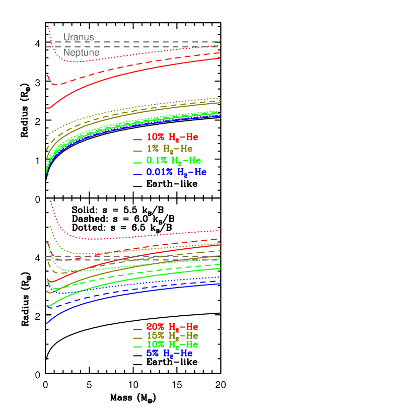
Figure 3.— Mass-radius curves of planets with Earth-like cores and gaseous envelopes. Top panel: envelopes equal to 0.01%, 0.1%, 1%, and 10% of the total mass. Bottom panel: envelopes equal to 5%, 10%, 15%, and 20% of the total mass. Curves with envelope entropies of 5.5, 6.0, and 6.5 $k_{B}$ per baryon ($k_{B}/B$) are plotted (assuming a convective envelope). An upturn in radius at low mass is apparent for larger envelope fractions. In the most extreme case of 20% H₂-He and $s=6.5k_{B}/B$, the minimum radius occurs at a mass of 5.5 M_⊕. The radii are very sensitive to the H₂-He fraction, but much less sensitive to the total mass of the planet, particularly for masses $>5$ M_⊕.

We now present new models of planets with H₂-He envelopes with both “Earth-like” rock-iron cores with 32.5% Fe and 67.5% MgSiO₃ (perovskite) and with pure water (Ice VII) cores. Ice cores are of particular interest because it may be the case that planets with significant gaseous envelopes and core masses form only beyond the snow line. We compute models with varying envelope masses from 0 to 10 M_⊕ and envelope entropies ranging from 5.5 to 6.5 $k_{B}$ per baryon ($k_{B}/B$)$-$in most cases, using discrete values of 5.5, 6.0, and 6.5 $k_{B}$ per baryon. These values are comparable to the entropies found by the evolutionary models of 2013arXiv1311.0329L for planets of Gyr age or older (specifically, Solar-metallicity models fall entirely within this range for $t>1$ Gyr, and 50x Solar enhanced-opacity models fall entirely within this range for $t>4$ Gyr).

In this section, we present models with a fully convective envelope, i.e., models with only a thin radiative atmosphere. This is a good approximation to Uranus and Neptune, where the radiative-convective boundary is at $<1$ bar (2013arXiv1312.3323S), and the equilibrium temperature is $\sim 50$ K, resulting in a small scale height. However, it is not a good approximation for highly-irradiated planets, for which the radiative-convective boundary is at a high pressure of $\sim 1000$ bar (2013arXiv1312.3323S) and the equilibrium temperature is much larger. The depth of the radiative atmosphere varies widely depending on the irradtion level and surface gravity. We investigate the effect of this radiative atmosphere on computed masses and radii in Section 4.

In Figure 3, we plot radius versus total mass for planets with Earth-like cores and H₂-He envelope with mass fractions ranging from 0.01% to 20%. The code produces results consistent with the known properties of Uranus and Neptune ($\sim$10% H₂-He) and also reproduces the upturn in radius at low masses for envelopes comprising $\geq 5\%$ of the total mass, which was produced by 2011ApJ...738...59R. Figure 3 also shows that the mass-radius curves are only slowly-rising for total masses $\gtrsim$5 M_⊕, i.e. radius is not strongly dependent on total mass, while it is more strongly dependent on the mass fraction and entropy in the H₂-He envelope.

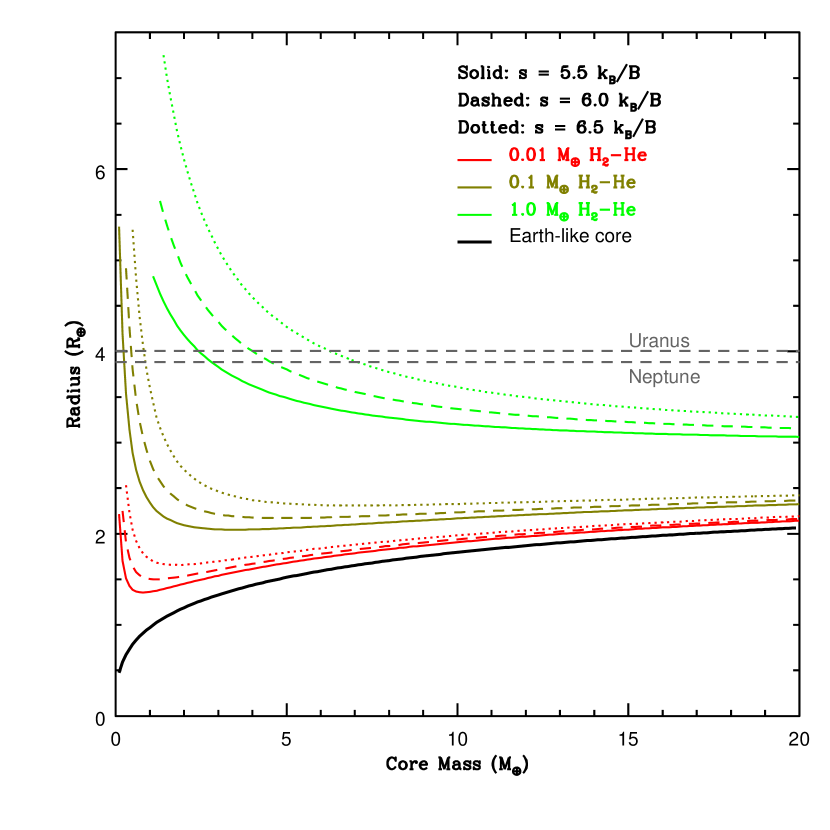
Figure 4.— Radius versus core mass for planets with constant envelope masses of 0.01, 0.1, and 1.0 M_⊕. Curves with envelope entropies of 5.5, 6.0, and 6.5 $k_{B}/B$ are plotted. The curves are remarkably flat for core masses greater than $\sim$5 M_⊕, indicating that the properties of the core have little influence on the observable properties of all but the smallest known planets.

Alternatively, in Figure 4, we plot radius versus core mass, rather than total mass, for constant envelope masses of 0.01, 0.1, and 1.0 M_⊕. Here, we see that for lower-mass cores ($\lesssim$5 M_⊕), the planetary radius is quite sensitive to core mass and entropy, but for higher-mass cores ($\gtrsim$5 M_⊕), which cover most current planet observations, the radius is most sensitive to envelope mass alone and varies very little with core mass, even less than with total mass. This suggests that mass-radius observations can be used to determine the core-envelope decomposition for a planet more precisely than the envelope mass fraction. In particular, because mass measurements usually have much larger uncertainties than radius measurements, it will be possible in many cases to determine envelope mass with more precision than mass fraction, which will have useful applications in formation models. In Table 7, we provide a sample table of properties of these models as a function of $M_{c}$ for $M_{env}=0.1$ M_⊕ and $s=6.0k_{B}$ per baryon.

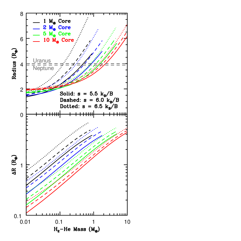
Figure 5.— Top panel: radius versus envelope mass for planets with constant core masses of 1, 2, 5, and 10 M_⊕. Bottom panel: Envelope depth ($\Delta R=R_{p}-R_{c}$) versus envelope mass. Curves with entropies of 5.5, 6.0, and 6.5 $k_{B}/B$ are plotted. Envelope depth follows a power law in terms of envelope mass, $\Delta R\propto M_{env}^{x}$, where $x=0.523-0.577$.

For comparison, in the top panel of Figure 5, we plot radius versus envelope mass for models with constant core masses of 1, 2, 5, and 10 M_⊕. Here, again, we see that for lower-mass cores (1 and 2 M_⊕), the planetary radius is quite sensitive to core mass and envelope entropy, but, for higher-mass cores (5 and 10 M_⊕), radius is most sensitive to envelope mass.

We also note that the curves are relatively flat for envelopes with masses $\lesssim$0.1 M_⊕, in which case the radius of the solid core dominates the total radius. However, we see another useful relation in the bottom panel of Figure 5, where we plot the envelope depth, $\Delta R=R_{p}-R_{c}$, versus envelope mass. In all cases, the envelope depth follows an approximate power law with core mass and envelope mass: $\Delta R\propto M_{env}^{x}M_{c}^{y}$. While the curves are bent to a slightly shallower slope at both low and high masses, the power-law indices over most of their lengths fall within a narrow range for $x$, $x=0.523\rightarrow 0.577$, but a wider range for $y$, $y=-0.565\rightarrow-0.693$. We provide tables of the properties of representative models from this plot in Tables 8-12.

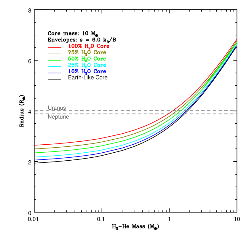
Figure 6.— Radius versus envelope mass for planets with 10-M_⊕ cores containing water layers (in the form of Ice VII) with mass fractions of 0%, 10%, 25%, 50%, 75%, and 100%. Envelope entropy is set to 6.0 $k_{B}/B$.

In Figure 6, we plot radius versus envelope mass for models with a constant core mass, 10 M_⊕, and entropy, $s=6.0\,k_{B}$ per baryon, but varying water fraction in the core$-$using a core structure with iron and silicate layers surrounded by a water (Ice VII) layer, comprision a varying fraction of the core mass from no water content to a pure ice core. The effect of the water fraction on radius is dominant in planets with small gaseous envelopes of $\lesssim 1$ M_⊕. For larger envelopes, the envelope mass becomes more important, and the variation with water fraction shrinks. Changing the water abundance of the core causes the total radius of the planet to vary by up to about 30% if the envelope mass is small (so the effect of the change in the core radius is strong), but by only about 10% for larger envelopes, $M_{env}\rightarrow 10$ M_⊕, less than the effect of varying the entropy for envelopes of these masses.

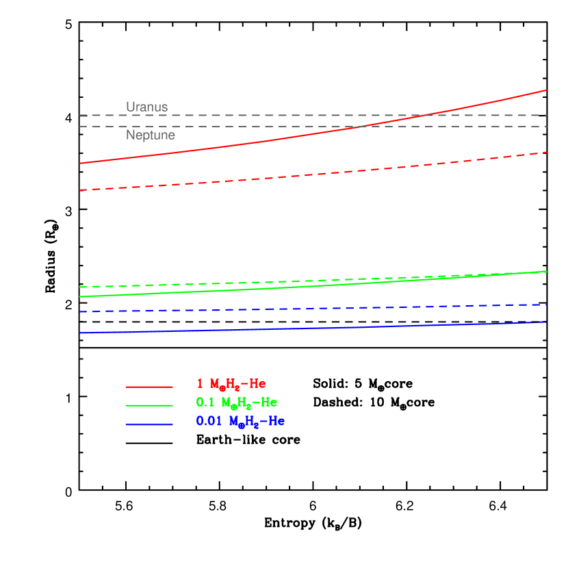
Figure 7.— Radius versus entropy for planets with core masses of 5 and 10 M_⊕. Curves with envelope masses of 0.01, 0.1, and 1.0 M_⊕ are plotted. Entropy becomes a significant influence on the radius for large envelopes.

In Figure 7, we set constant core masses of 5 and 10 M_⊕ and plot radius versus entropy for constant envelope masses of 0.01, 0.1, and 1.0 M_⊕. The radius is relatively insensitive to entropy for the lower envelope masses, but entropy becomes significant for envelopes with masses $\gtrsim$1 M_⊕.

4. Fits to Known Planets

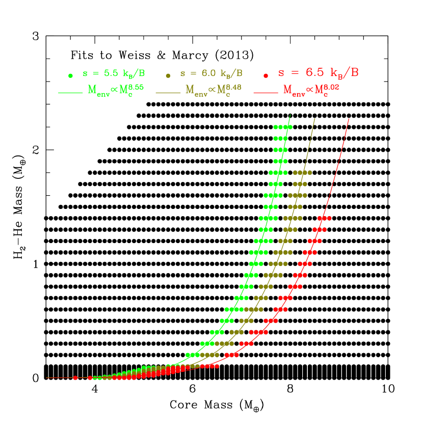
Figure 8.— The functional mass-radius fit of 2014ApJ...783L...6W plotted through a data cube of our planet models (points) with varying entropy, core mass, and envelope mass, for Earth-like (iron-silicate) cores. Colored points lie within 0.2 M_⊕ of this functional fit for an envelope entropy of 5.5 (green), 6.0 (yellow), and 6.5 (red) $k_{B}/B$. We fit a power law (shown) in (core mass)-(envelope mass) space to the functional fit for each entropy.

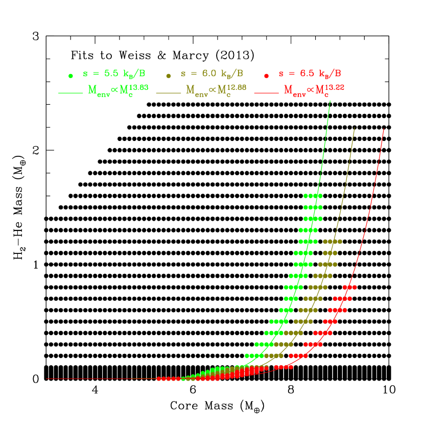
Figure 9.— Same as Figure 8, but for pure ice cores.

2014ApJ...783L...6W fit a two-piece mass-radius function to 65 low-mass planets with radii $\leq 4$ R_⊕ and masses measured by 2014ApJS..210...20M. For planets with radii $<1.5$ R_⊕, they fit an Earth-like model defined by the density formula $\rho=2.43+3.39R$, where $\rho$ is the density in g cm^-3 and $R$ is the radius in Earth radii. For planets with radii $>1.5$ R_⊕, they apply a model of increasing H₂-He fraction with mass with a (nearly-linear) power law fit: $M=2.69R^{0.93}$, where $M$ and $R$ are given in Earth masses and radii.

We fit these mass-radius fits to a data cube of our models with varying entropy, core mass, and envelope mass in Figures 8 and 9. Ambiguities in metallicity, age, and heat redistribution make it difficult to investigate the exact structures of individual planets, so we seek to bracket the range of possibilities with different core compositions and entropies. In Figure 8 we employ models with Earth-like cores (32.5% Fe and 67.5% MgSiO₃), and in Figure 9, we employ models with pure water (Ice VII) cores. We plot each of our models as a point in (core mass)-(envelope mass) space. Each point corresponds to a particular total mass and a range of radii, depending on the envelope entropy. By setting the entropy to 5.5 (green), 6.0 (yellow), and 6.5 (red) $k_{B}$ per baryon, we highlight those points that lie within 0.2 M_⊕ of the mass-radius fit derived by 2014ApJ...783L...6W. Following these highlighted points, we fit power laws in (core mass)-(envelope mass) space to the functional fit at each entropy. In general, we find a good fit to a power law, $M_{env}\propto M_{c}^{x}$, where $x=8.0-8.5$ for rock-iron cores and $x=13-14$ for pure ice cores, a very steep dependence of envelope mass on core mass.

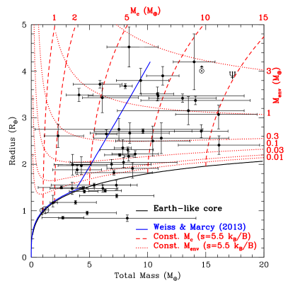
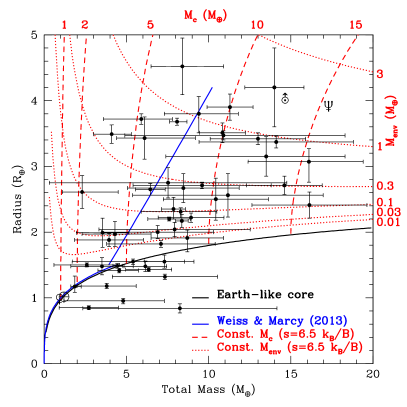
Figure 10.— Known extrasolar planets plotted against the observational mass-radius fits of 2014ApJ...783L...6W (blue) and a grid of constant core mass and envelope mass curves (red) for planets with Earth-like (iron-silicate) cores. Curves with entropies of 5.5 and 6.5 $k_{B}/B$ are plotted.

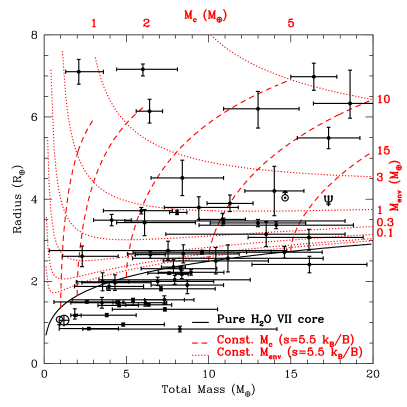
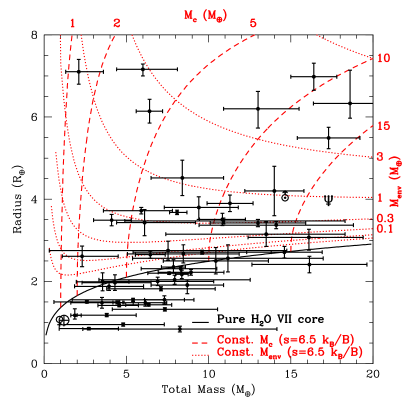
Figure 11.— Same as Figure 10, but for pure ice cores. The functional fit has been omitted.

Table 2Masses and Radii of Observed Exoplanets and Theoretical Decomposition into Core and Convective Envelope Components ($s=6.0k_{B}/B$)

Planet	Radius (R⊕)	Mass (M⊕)	$M_{c}$ (M⊕)	$M_{env}$ (M⊕)	$M_{c}$ (M⊕)	$M_{env}$ (M⊕)	References
			(Fe/Rock Core)	(Fe/Rock Core)	(H2O Core)	(H2O Core)
55 Cancri e	$2.17\pm 0.10$	$8.37\pm 0.38$	8.284	0.086	8.37	0.00	1,2
CoRoT-7b	$1.55\pm 0.10$	$7.31\pm 1.21$	7.31	0.00	7.31	0.00	3
GJ 1214b	$2.65\pm 0.09$	$6.45\pm 0.91$	6.15	0.30	6.396	0.054	4
GJ 3470b	$4.20\pm 0.60$	$14.0\pm 1.8$	11.6	2.4	12.5	1.5	5
HAT-P-26b	$6.33_{-0.36}^{+0.81}$	$18.60\pm 2.22$	9.9	8.7	10.9	7.7	6
HD 97658b	$2.35_{-0.15}^{+0.18}$	$7.86\pm 0.73$	7.50	0.36	7.86	0.00	7
Kepler-10b	$1.416_{-0.036}^{+0.033}$	$4.56_{-1.29}^{+1.17}$	4.56	0.00	4.56	0.00	8
Kepler-11b	$1.97\pm 0.19$	$4.3_{-2.0}^{+2.2}$	4.247	0.053	4.3	0.00	9
Kepler-11c	$3.15\pm 0.30$	$13.5_{-6.1}^{+4.8}$	12.66	0.84	13.32	0.18	9
Kepler-11d	$3.43\pm 0.32$	$6.1_{-1.7}^{+3.1}$	5.35	0.75	5.67	0.43	9
Kepler-11e	$4.52\pm 0.43$	$8.4_{-1.9}^{+2.5}$	6.3	2.1	6.8	1.6	9
Kepler-11f	$2.61\pm 0.25$	$2.3_{-1.2}^{+2.2}$	2.14	0.16	2.226	0.074	9
Kepler-18b	$2.00\pm 0.10$	$6.9\pm 3.4$	6.856	0.044	6.9	0.00	10
Kepler-18c	$5.49\pm 0.26$	$17.3\pm 1.9$	11.5	5.8	12.5	4.8	10
Kepler-18d	$6.98\pm 0.33$	$16.4\pm 1.4$			7.3	9.1	10
Kepler-20b	$1.91_{-0.21}^{+0.12}$	$8.7\pm 2.2$	8.688	0.012	8.7	0.00	11
Kepler-20c	$3.07_{-0.31}^{+0.20}$	$16.1_{-3.7}^{+3.3}$	15.30	0.80	16.002	0.098	11
Kepler-20d	$2.75\pm 0.23$	$7.53\pm 7.22$	7.16	0.37	7.461	0.069	12
Kepler-25b	$2.71\pm 0.05$	$9.6\pm 4.2$	9.23	0.37	9.572	0.028	12
Kepler-30b	$3.90\pm 0.20$	$11.3\pm 1.4$	9.6	1.7	10.31	0.99	13
Kepler-36b	$1.486\pm 0.035$	$4.45_{-0.27}^{+0.33}$	4.45	0.00	4.45	0.00	14
Kepler-36c	$3.679\pm 0.054$	$8.08_{-0.46}^{+0.60}$	6.96	1.12	7.41	0.67	14
Kepler-48b	$1.88\pm 0.10$	$3.94\pm 2.10$	3.902	0.038	3.94	0.00	12
Kepler-48c	$2.71\pm 0.14$	$14.61\pm 2.30$	14.21	0.40	14.61	0.00	12
Kepler-48d	$2.04\pm 0.11$	$7.93\pm 4.60$	7.883	0.047	7.93	0.00	12
Kepler-50b	$2.20\pm 0.03$	$7.6\pm 1.3$	7.5	0.10	7.6	0.00	15
Kepler-51b	$7.10\pm 0.30$	$2.1_{-0.80}^{+1.50}$			0.84	1.26	16
Kepler-57c	$1.55\pm 0.04$	$5.4\pm 3.7$	5.4	0.00	5.4	0.00	15
Kepler-68b	$2.31_{-0.09}^{+0.06}$	$8.3_{-2.4}^{+2.2}$	8.16	0.14	8.3	0.00	17
Kepler-68c	$0.953_{-0.042}^{+0.037}$	$4.8_{-3.6}^{+2.5}$	4.8	0.00	4.8	0.00	17
Kepler-78b	$1.173_{-0.089}^{+0.159}$	$1.86_{-0.25}^{0.38}$	1.86	0.00	1.86	0.00	18
Kepler-79b	$3.47\pm 0.07$	$10.9_{-6.0}^{7.4}$	9.79	1.11	10.4	0.50	19
Kepler-79c	$3.72\pm 0.08$	$5.9_{-2.3}^{1.9}$	4.97	0.93	5.28	0.62	19
Kepler-79d	$7.16_{-0.16}^{+0.13}$	$6.0_{-1.6}^{2.1}$			2.0	4.0	19
Kepler-79e	$3.49\pm 0.14$	$4.1_{-1.1}^{1.2}$	3.51	0.59	3.71	0.39	19
Kepler-87c	$6.14\pm 0.29$	$6.4\pm 0.8$			3.3	3.1	20
Kepler-89c	$3.80_{-0.29}^{+0.26}$	$9.4_{-2.1}^{-2.4}$	8.0	1.4	8.58	0.82	21
Kepler-89e	$6.20_{-0.47}^{+0.42}$	$13.0_{-2.1}^{-2.5}$			7.3	5.7	21
Kepler-93b	$1.50\pm 0.03$	$2.59\pm 2.00$	2.585	0.005	2.59	0.00	12
Kepler-94b	$3.51\pm 0.15$	$10.84\pm 1.40$	9.69	1.15	10.30	0.54	12
Kepler-95b	$3.42\pm 0.09$	$13.0\pm 2.9$	11.85	1.15	12.57	0.43	12
Kepler-96b	$2.67\pm 2.22$	$8.46\pm 3.40$	8.12	0.34	8.428	0.032	12
Kepler-97b	$1.48\pm 0.13$	$3.51\pm 1.90$	3.509	0.001	3.51	0.00	12
Kepler-98b	$1.99\pm 0.22$	$3.55\pm 1.60$	3.491	0.059	3.5496	0.0004	12
Kepler-99b	$1.48\pm 0.08$	$6.15\pm 1.30$	6.15	0.00	6.15	0.00	12
Kepler-100b	$1.32\pm 0.04$	$7.34\pm 3.20$	7.34	0.00	7.34	0.00	12
Kepler-102b	$1.18\pm 0.04$	$3.8\pm 1.8$	3.8	0.00	3.8	0.00	12
Kepler-102e	$2.22\pm 0.07$	$8.93\pm 2.00$	8.83	0.10	8.93	0.00	12
Kepler-103b	$3.37\pm 0.09$	$14.11\pm 4.70$	12.97	1.14	13.75	0.36	12
Kepler-106c	$2.50\pm 0.32$	$10.44\pm 3.20$	10.20	0.24	10.44	0.00	12
Kepler-106e	$2.56\pm 0.33$	$11.17\pm 5.80$	10.89	0.28	11.17	0.00	12
Kepler-113b	$1.82\pm 0.05$	$7.1\pm 3.3$	7.091	0.009	7.1	0.00	12
Kepler-131b	$2.41\pm 0.20$	$16.13\pm 3.50$	15.98	0.15	16.13	0.00	12
Kepler-131c	$0.84\pm 0.07$	$8.25\pm 5.90$	8.25	0.00	8.25	0.00	12
Kepler-406b	$1.43\pm 0.03$	$6.35\pm 1.40$	6.35	0.00	6.35	0.00	12
Kepler-406c	$0.85\pm 0.03$	$2.71\pm 0.80$	2.71	0.00	2.71	0.00	12
Uranus	4.007	14.536	12.436	2.1	13.336	1.2
Neptune	3.883	17.147	15.047	2.1	16.147	1.0

Table 3Masses and Radii of Observed Exoplanets and Theoretical Decomposition into Core and Convective Envelope Components ($s=6.0k_{B}/B$) with Radii Corrected for the Thickness ($\Delta R$) of the Radiative Atmosphere

Planet	Radius (R⊕)	Mass (M⊕)	$\Delta R$ (R⊕)	$M_{c}$ (M⊕)	$M_{env}$ (M⊕)	$M_{c}$ (M⊕)	$M_{env}$ (M⊕)	References
				(Fe/Rock Core)	(Fe/Rock Core)	(H2O Core)	(H2O Core)
55 Cancri e	$2.17\pm 0.10$	$8.37\pm 0.38$	0.523	8.37	0.00	8.37	0.00	1,2
CoRoT-7b	$1.55\pm 0.10$	$7.31\pm 1.21$	0.284	7.31	0.00	7.31	0.00	3
GJ 1214b	$2.65\pm 0.09$	$6.45\pm 0.91$	0.294	6.27	0.18	6.444	0.006	4
GJ 3470b	$4.20\pm 0.60$	$14.0\pm 1.8$	0.370	12.1	1.9	12.98	1.02	5
HAT-P-26b	$6.33_{-0.36}^{+0.81}$	$18.60\pm 2.22$	1.027	12.7	5.9	13.9	4.7	6
HD 97658b	$2.35_{-0.15}^{+0.18}$	$7.86\pm 0.73$	0.246	7.782	0.078	7.86	0.00	7
Kepler-10b	$1.416_{-0.036}^{+0.033}$	$4.56_{-1.29}^{+1.17}$	0.455	4.56	0.00	4.56	0.00	8
Kepler-11b	$1.97\pm 0.19$	$4.3_{-2.0}^{+2.2}$	0.405	4.297	0.003	4.3	0.00	9
Kepler-11c	$3.15\pm 0.30$	$13.5_{-6.1}^{+4.8}$	0.301	12.94	0.56	13.469	0.031	9
Kepler-11d	$3.43\pm 0.32$	$6.1_{-1.7}^{+3.1}$	0.660	5.71	0.39	5.98	0.12	9
Kepler-11e	$4.52\pm 0.43$	$8.4_{-1.9}^{+2.5}$	0.756	7.1	1.3	7.55	0.85	9
Kepler-11f	$2.61\pm 0.25$	$2.3_{-1.2}^{+2.2}$	0.798	2.257	0.043	2.298	0.002	9
Kepler-18b	$2.00\pm 0.10$	$6.9\pm 3.4$	0.356	6.9	0.00	6.9	0.00	10
Kepler-18c	$5.49\pm 0.26$	$17.3\pm 1.9$	0.826	13.4	3.9	14.5	2.8	10
Kepler-18d	$6.98\pm 0.33$	$16.4\pm 1.4$	1.128	9.5	6.9	10.4	6.0	10
Kepler-20b	$1.91_{-0.21}^{+0.12}$	$8.7\pm 2.2$	0.241	8.7	0.00	8.7	0.00	11
Kepler-20c	$3.07_{-0.31}^{+0.20}$	$16.1_{-3.7}^{+3.3}$	0.234	15.44	0.56	16.095	0.005	11
Kepler-20d	$2.75\pm 0.23$	$7.53\pm 7.22$	0.209	7.25	0.28	7.506	0.024	12
Kepler-25b	$2.71\pm 0.05$	$9.6\pm 4.2$	0.517	9.501	0.099	9.6	0.00	12
Kepler-30b	$3.90\pm 0.20$	$11.3\pm 1.4$	0.383	10.0	1.3	10.69	0.61	13
Kepler-36b	$1.486\pm 0.035$	$4.45_{-0.27}^{+0.33}$	0.254	4.45	0.00	4.45	0.00	14
Kepler-36c	$3.679\pm 0.054$	$8.08_{-0.46}^{+0.60}$	0.815	7.58	0.50	7.95	0.13	14
Kepler-48b	$1.88\pm 0.10$	$3.94\pm 2.10$	0.430	3.9398	0.0002	3.94	0.00	12
Kepler-48c	$2.71\pm 0.14$	$14.61\pm 2.30$	0.260	14.40	0.21	14.61	0.00	12
Kepler-48d	$2.04\pm 0.11$	$7.93\pm 4.60$	0.135	7.909	0.021	7.93	0.00	12
Kepler-50b	$2.20\pm 0.03$	$7.6\pm 1.3$						15
Kepler-51b	$7.10\pm 0.30$	$2.1_{-0.80}^{+1.50}$						16
Kepler-57c	$1.55\pm 0.04$	$5.4\pm 3.7$						15
Kepler-68b	$2.31_{-0.09}^{+0.06}$	$8.3_{-2.4}^{+2.2}$	0.384	8.277	0.023	8.3	0.00	17
Kepler-68c	$0.953_{-0.042}^{+0.037}$	$4.8_{-3.6}^{+2.5}$	0.093	4.8	0.00	4.8	0.00	17
Kepler-78b	$1.173_{-0.089}^{+0.159}$	$1.86_{-0.25}^{0.38}$	0.733	1.86	0.00	1.86	0.00	18
Kepler-79b	$3.47\pm 0.07$	$10.9_{-6.0}^{7.4}$	0.522	10.28	0.62	10.78	0.12	19
Kepler-79c	$3.72\pm 0.08$	$5.9_{-2.3}^{1.9}$	0.877	5.48	0.42	5.74	0.16	19
Kepler-79d	$7.16_{-0.16}^{+0.13}$	$6.0_{-1.6}^{2.1}$	2.586	4.3	1.7	4.5	1.5	19
Kepler-79e	$3.49\pm 0.14$	$4.1_{-1.1}^{1.2}$	0.776	3.80	0.30	3.97	0.13	19
Kepler-87c	$6.14\pm 0.29$	$6.4\pm 0.8$	1.456	4.5	1.9	4.7	1.7	20
Kepler-89c	$3.80_{-0.29}^{+0.26}$	$9.4_{-2.1}^{-2.4}$	0.799	8.76	0.64	9.21	0.19	21
Kepler-89e	$6.20_{-0.47}^{+0.42}$	$13.0_{-2.1}^{-2.5}$	0.887	8.4	4.6	9.1	3.9	21
Kepler-93b	$1.50\pm 0.03$	$2.59\pm 2.00$	0.444	2.59	0.00	2.59	0.00	12
Kepler-94b	$3.51\pm 0.15$	$10.84\pm 1.40$	0.574	10.23	0.61	10.72	0.12	12
Kepler-95b	$3.42\pm 0.09$	$13.0\pm 2.9$	0.438	12.31	0.69	12.90	0.10	12
Kepler-96b	$2.67\pm 2.22$	$8.46\pm 3.40$	0.328	8.29	0.17	8.46	0.00	12
Kepler-97b	$1.48\pm 0.13$	$3.51\pm 1.90$	0.447	3.51	0.00	3.51	0.00	12
Kepler-98b	$1.99\pm 0.22$	$3.55\pm 1.60$	0.937	3.55	0.00	3.55	0.00	12
Kepler-99b	$1.48\pm 0.08$	$6.15\pm 1.30$	0.146	6.15	0.00	6.15	0.00	12
Kepler-100b	$1.32\pm 0.04$	$7.34\pm 3.20$	0.147	7.34	0.00	7.34	0.00	12
Kepler-102b	$1.18\pm 0.04$	$3.8\pm 1.8$	0.145	3.8	0.00	3.8	0.00	12
Kepler-102e	$2.22\pm 0.07$	$8.93\pm 2.00$	0.149	8.873	0.057	8.93	0.00	12
Kepler-103b	$3.37\pm 0.09$	$14.11\pm 4.70$	0.354	13.37	0.74	14.01	0.10	12
Kepler-106c	$2.50\pm 0.32$	$10.44\pm 3.20$	0.241	10.32	0.12	10.44	0.00	12
Kepler-106e	$2.56\pm 0.33$	$11.17\pm 5.80$	0.156	10.97	0.20	11.17	0.00	12
Kepler-113b	$1.82\pm 0.05$	$7.1\pm 3.3$	0.175	7.1	0.00	7.1	0.00	12
Kepler-131b	$2.41\pm 0.20$	$16.13\pm 3.50$	0.139	16.047	0.083	16.13	0.00	12
Kepler-131c	$0.84\pm 0.07$	$8.25\pm 5.90$	0.026	8.25	0.00	8.25	0.00	12
Kepler-406b	$1.43\pm 0.03$	$6.35\pm 1.40$	0.221	6.35	0.00	6.35	0.00	12
Kepler-406c	$0.85\pm 0.03$	$2.71\pm 0.80$	0.146	2.71	0.00	2.71	0.00	12
Uranus	4.007	14.536	0.033	12.436	2.1	13.336	1.2
Neptune	3.883	17.147	0.021	15.047	2.1	16.147	1.0

However, 2014ApJ...783L...6W find an RMS deviation in mass around their fit of 4.3 M_⊕, which can easily lead to a factor of two or more variation in total mass at a given radius. To address this, in Figures 10 and 11, we demonstrate the power of the core-envelope decomposition by plotting known planets on a grid of constant-core-mass and constant-envelope-mass curves (red) for two entropies of 5.5 and 6.5 $k_{B}$ per baryon. In Figure 10, we employ models with Earth-like cores, and in Figure 11, we employ models with pure ice cores. With this grid, each mass-radius pair can be associated with a unique core mass and envelope mass for a given entropy and core type. The functional fit from 2014ApJ...783L...6W is also shown in blue in Figure 10.

Because of the larger radii of the ice cores, it takes significantly less envelope mass to produce the same radius for a given total mass. This allows us to extend Figure 11 to larger radii to reflect this, noting the detection of several more planets with large radii and envelope masses of $\sim 1-10$ M_⊕ in this case.

Figures 10 and 11 assume a fully convective envelope, which is a good approximation when irradiation is low, but not when irradiation is high, and the radiative atmosphere is deep. Depending on the irradation and surface gravity, the radiative atmosphere typically comprises 10%-20% of the planetary radius, significantly greater than the depth of a convective atmosphere reaching the pressure of the radiative-convective boundary, which results in a larger radius than a fully-convective envelope would suggest. 2014ApJ...783L...6W find a good fit to an approximation setting the depth of the radiative atmosphere to nine times the scale height (a radiative-convective boundary at 162 bar), and we apply this approximation to estimate the effect of including the radiative atmosphere in our model. The actual depth of the radiative-convective boundary will depend on irradiation, age, and metallicity.

We provide the quantitative core-envelope decomposition for observed exoplanets and Solar System planets in Tables 2 and 3 in both the rocky-iron core and ice core cases for an envelope entropy of 6.0 $k_{B}$ per baryon. Tables 2 gives the decomposition for a fully-convective envelope, and Table 3 gives the decomposition with the correction for the radiative atmosphere included. If the observed radius is smaller than a bare core of the observed mass for one or both core types, we still include the decomposition with an envelope mass of zero. Uranus and Neptune are included with both core types for comparison purposes.

The core-envelope decompositions readily reveal useful information about the structures of planets from mass-radius data. For example, in the fully convective case, the low-density planet Kepler-11e (the topmost point plotted in Figure 10), can be fit to a model with a large H₂-He fraction based on an Earth-like core mass of 6.3 M_⊕ and an envelope mass of 2.1 M_⊕, for an entropy for 6.0 $k_{B}$ per baryon, with small differences for a different entropy, or an icy core mass of 6.8 M_⊕ and envelope mass of 1.6 M_⊕. In contrast, the higher-density planet Kepler-131b (the bottom-rightmost point) can be fit to a model with a small H₂-He fraction based on an Earth-like core mass of 15.98 M_⊕ and an envelope mass of 0.15 M_⊕ at an entropy of 6.0 $k_{B}$ per baryon. For an ice core, the bare core would suffice.

The difference in envelope mass between an Earth-like core model and an ice core model can be as small as 0.059 M_⊕ while still retaining some envelope (e.g. Kepler-98b), but is usually a few tenths of an Earth mass. The largest difference of 1.1 M_⊕ occurs for Neptune.

When the correction for the radiative atmosphere is applied, the H₂-He mass fractions required to fit the measured masses and radii decrease significantly. A number of planets can be modeled as a solid core with only a radiative atmosphere (which in all cases has a mass fractions of $<10^{-4}$) and no convective envelope. At the other extreme, when modeled with an ice core, the low-density planet Kepler-18d has a hydrogen fraction of 55% assuming a fully convective envelope, but 35% given the correction for the radiative atmosphere, the largest H₂-He mass fraction of any planet we study in the latter case. The results given by 2012ApJ...761...59L for the Kepler-11 system are consistent with these corrected results for an Earth-like core, except for Kepler-11f, for which we predict a smaller envelope mass fraction.

We note a small number of planets with masses of 2$-$20 M_⊕ and very large radii (for these masses) of 5$-$7 R_⊕, such as Kepler-18d, as shown in Figure 11. While additional planet detections and further investigation with gas giant models is needed to investigate these objects in detail, we see from these objects that large envelope fractions can occur even for low-mass planets. Even including the radiative atmosphere correction, we find H₂-He mass fractions of 22%-35% for this population. (Without this correction, the H₂-He mass fractions are approximately twice as large.)

This core-envelope decomposition for observed planets, especially when the large-radius planets are included, implies that envelope mass can vary from zero to tens of percent of the total mass for the entire range of masses we study, except that we find a lower limit of envelope mass of $\sim$0.1 M_⊕ in the case of Earth-like cores with masses of $\sim 8-20$ M_⊕. More specifically, where a non-zero envelope mass is predicted, it can vary by two orders of magnitude for a similar core mass. While we do see the trend of decreasing density for masses $>7.6$ M_⊕ observed by 2014ApJ...783L...6W, with a broad scatter of the observed planets centered around the functional fit, the spread in core mass and envelope mass is so wide that we see only a slight justification for any given functional fit.

We consider the possibility of multiple populations of planets in envelope mass space$-$one with $M_{env}\gtrsim$3 M_⊕, one with $M_{env}\sim 1$ M_⊕, and one with $M_{env}\lesssim 0.3$ M_⊕, but the statistics are not sufficient to tell whether these populations are distinct. In any case, it is clear that a significant amount of H₂-He ($\sim$1 M_⊕) is needed to produce the large radii observed for many low-mass planets. We also note that many of the newly-discovered planets fall in the 5$-$10 M_⊕ core mass range, but, again, it is not clear if this genuinely reflects the true underlying distribution function, or is due to statistics and selection biases.

5. Uncertainty Range

Table 4Computed Envelope Masses for Selected Planets From Different Models

	Kepler-98b	Kepler-11f	Kepler-25b	Kepler-20c	Kepler-11e	HAT-P-26b
Mass	$3.55\pm 1.60$	$2.3_{-1.2}^{+2.2}$	$9.6\pm 4.2$	$16.1_{-3.7}^{+3.3}$	$8.4_{-1.9}^{+2.5}$	$18.60\pm 2.22$
Radius	$1.99\pm 0.22$	$2.61\pm 0.25$	$2.71\pm 0.05$	$3.07_{-0.31}^{+0.20}$	$4.52\pm 0.43$	$6.33_{-0.36}^{+0.81}$
$\Delta R$	0.937	0.798	0.517	0.234	0.756	1.027
Purely Convective Models
Rock-Iron Core, s=5.51	0.086	0.230	0.47	0.95	2.6
Rock-Iron Core, s=6.5	0.035	0.097	0.28	0.64	1.6	7.2
Ice Core, s=5.5	0.0008	0.125	0.049	0.123	2.1	9.2
Ice Core, s=6.5	0.0003	0.038	0.014	0.044	1.1	6.2
Models With Radiative Atmsophere
Rock-Iron Core, s=5.5	0.00	0.061	0.127	0.66	1.6	6.7
Rock-Iron Core, s=6.5	0.00	0.027	0.069	0.45	1.0	5.0
Ice Core, s=5.5	0.00	0.003	0.00	0.006	1.10	5.5
Ice Core, s=6.5	0.00	0.001	0.00	0.003	0.62	3.8

¹Entropies are given in units of $k_{B}$ per baryon.

All of the model parameters we consider$-$envelope entropy, core composition, and the depth of the radiative atmosphere$-$have effects on our computed core-envelope decompositions. Tables 10 and 11 explore the limiting cases for core composition, that is, rock-iron cores and pure ice cores, as well as the limiting cases for the correction for the radiative atmosphere, that is, no correction versus a suggested upper bound of the depth of nine scale heights, as fit by 2013arXiv1311.0329L. To provide a picture of the uncertainties involved in our modeling of exoplanets, we compute in Table 4 the envelope masses for selected exoplanets that populate a large part of the mass-radius space, listed in order of increasing radius. In this table, we compute envelope masses for the above parameters as well as envelope entropies of 5.5 and 6.5 $k_{B}$ per baryon, which bracket the expected range of entropies predicted by 2013arXiv1311.0329L. In Tables 10 and 11, we compute models with only $s=6.0\,k_{B}$ per baryon.

There is not a simple empirical rule for the trends in our results, but several important features can be seen. Most notably, we may consider very roughly two categories of objects: those with relatively small radii that can only be fit with low-mass envelopes (e.g., Kepler-98b) and those with relatively large radii that can only be fit with high-mass envelopes (e.g., HAT-P-26b). These categories are arbitrary, since the population is essentially a continuum with objects like Kepler-20c stradling the boundary, but they serve to illustrate the limits we can place on individual objects and the effects of varying the parameters. The behavior of each parameter is significantly different in the two categories.

The correction for the presence of the radiative atmosphere reduces the convective envelope masses needed to fit the mass and radius data. For planets that have especially low-mass envelopes without the correction, this can go to zero, that is, only the (much lower mass) radiative atmosphere is needed. This can be seen with 55 Cancri e (envelope mass 0.086 M_⊕ for $s=6.0\,k_{B}$ per baryon and a rock-iron core) and Kepler-98b (envelope mass 0.086 M_⊕ for $s=5.5\,k_{B}$ per baryon and a rock-iron core). However, other planets with similarly small envelopes still require a small, but non-zero envelope mass to fit the observational data, which may be more than an order of magnitude smaller than without the correction. For example, for $s=6.0\,k_{B}$ per baryon and a rock-iron core, Kepler-11b requires an envelope mass of 0.053 M_⊕ without the correction and 0.003 M_⊕ with it. In other cases a range of values may be required that nevertheless all remain relatively small ($\lesssim 0.5$ M_⊕), such as in the case of Kepler-79e, where we see envelope masses of 0.59 and 0.39 M_⊕ without the correction for the two different core types (rock-iron and ice, respectively), and corresponding masses of 0.30 and 0.13 M_⊕ with the correction. We typically find differences in envelope mass of 0.1-0.4 M_⊕ due to this correction for planets in this category.

On the other hand, planets for which the envelope mass is relatively large ($\gtrsim 1$ M_⊕) are modeled with large envelopes regardless of the parameters of the model. For example, for $s=6.0\,k_{B}$ per baryon, Kepler-18c requires an envelope mass of 5.8 M_⊕ for a rock-iron core and 4.8 M_⊕ for an ice core without the correction for the radiative atmosphere. With the correction, these values are 3.9 M_⊕ and 2.8 M_⊕, respectively. Similarly, without the correction, for HAT-P-26b with $s=6.0\,k_{B}$ per baryon, our modeled envelope mass is 8.7 M_⊕ for a rock-iron core and 7.7 M_⊕ for an ice core. With the correction, these values are 5.9 M_⊕ and 4.7 M_⊕, respectively$-$somewhat larger differences. On the other hand, without the correction, for GJ 3470b with $s=6.0\,k_{B}$ per baryon, our modeled envelope mass is 2.4 M_⊕ for a rock-iron core and 1.5 M_⊕ for an ice core. With the correction, these values are 1.9 M_⊕ and 1.02 M_⊕, meaning that the effect of the correction is significantly smaller in absolute terms. In general, we find that the correction for the radiative envelope reduces the envelope mass by 30%-50% for planets with large envelopes. The exceptions to this are Uranus and Neptune, for which the scale height is much smaller, and the radiative atmosphere makes a negligible contribution to the radius.

We can do a similar analysis of the effect of changing from a rock-iron core to a pure ice core. Because of the larger core radius, the need for a convective envelope can disappear for the ice core. If there is no radiative atmosphere, this corresponds to the bare core. The most extreme case of this is Kepler-48c, which requires an envelope mass of 0.40 M_⊕ to fit a rock-iron core with $s=6.0\,k_{B}$ per baryon and no radiative atmosphere, but no envelope to fit an ice core with otherwise the same parameters. For planets with small envelopes, we typically find differences in envelope mass of 0.2-0.5 M_⊕ for the different core types. For example, for Kepler-79e with $s=6.0\,k_{B}$ per baryon and no radiative atmosphere, the envelope mass falls from 0.59 M_⊕ to 0.39 M_⊕ when switching from a rock-iron core to an ice core. The values for the same models for Kepler-11c are 0.84 M_⊕ and 0.18 M_⊕, respectively.

For planets with large envelopes, we typically find differences in envelope mass of $\sim 1$ M_⊕ between models with a rock-iron core and an ice core. For example, with $s=6.0\,k_{B}$ per baryon and no radiative atmosphere, the respective envelope masses are 8.7 M_⊕ and 7.7 M_⊕ for HAT-P-26b, and 5.8 M_⊕ and 4.8_⊕ for Kepler-18c. With the correction for the radiative atmosphere, we find 1.9 M_⊕ and 1.02 M_⊕ for GJ 3470b, and 4.6 $M_{\earth}$ and 3.9 M_⊕ for Kepler-89e.

Table 4 shows the effect of varying the entropy of the envelope. Varying only the entropy cannot eliminate the need for a convective envelope because this depends on the core radius and the depth of the radiative atmosphere, which do not depend on the entropy. Instead, we see the masses of small envelopes vary by a factor of 2-3 over an entropy range of 5.5 to 6.5 $k_{B}$ per baryon, e.g., from 0.086 M_⊕ to 0.035 M_⊕, respectively, for Kepler-98b with a rock-iron core and no radiative atmosphere, from 0.230 M_⊕ to 0.097 M_⊕ for the same parameters for Kepler-11f, and from 0.47 M_⊕ to 0.28 M_⊕ for the same parameters for Kepler-25b.

For planets with larger envelopes, the variation in envelope mass over this entropy range is 30%-50%. For example, for Kepler-11e with a rock-iron core and no radiative atmosphere, we find envelope masses of 2.6 M_⊕ for $s=5.5k_{B}$ per baryon and 1.6M _⊕ for $6.5k_{B}$ per baryon. For an ice core, we similarly find values of 2.1 M_⊕ and 1.1$M_{\earth}$, respectively. For HAT-P-26b with an ice core and the correction for the radiative atmosphere, the respective masses are 5.5 M_⊕ and 3.8 M_⊕.

We do not expect planets of Gyr ages to fall significantly outside the range of $5.5-6.5\,k_{B}$ per baryon. However, we find that the inferred envelope masses for a given mass and radius in our models decrease roughly linearly with increasing entropy, so that a very wide possible entropy might result in a range of envelope masses of a factor of 2, still of similar magnitude to the effects of the other uncertainties. For example, we compute envelope masses for Kepler-11e with a rock-iron core and a radiative atmosphere for an entropy range of $4.3-7.0k_{B}$ per baryon. In this case, we compute envelope masses of 2.1 M_⊕ for an entropy of $4.3k_{B}$ per baryon, 1.6 M_⊕ for an entropy of 5.0 $k_{B}$ per baryon, 1.3 M_⊕ for an entropy of 6.0 $k_{B}$ per baryon, and 0.8 M_⊕ for an entropy of 7.0 $k_{B}$ per baryon.

Table 4 also allows us to bracket the envelope masses provided by all of our combinations of parameters, i.e., the combined effect of varying all three of the above parameters. Again, the minimum envelope mass required to fit the mass-radius data may be zero when considering all of the models, as for Kepler-98b and Kepler-25b, or small, but non-zero, e.g., 0.001 M_⊕ for Kepler-11f. Meanwhile, the largest envelope masses provided by any of the eight limiting cases of the variation of the three parameters (invariably $s=5.5k_{B}$ per baryon, rock-iron core, and no radiative atmosphere) are 0.086 M_⊕ for Kepler-98b, 0.230 for Kepler-11f, and 0.47 for Kepler-25b. Even with the effects of the three parameters combined, we see a range of relatively small envelope masses, e.g. 0.00-0.47 M_⊕, for objects with smaller radii.

For planets with large envelopes, we see a range of envelope masses, but they are invariably relatively large. The smallest envelope mass produced by any of our models for Kepler-11e is 0.62 M_⊕, while the largest is 2.6 M_⊕. Alternatively, we may express this as an envelope mass of $1.6\pm 1.0$ M_⊕, a range that accounts for all of the uncertainties in the parameters of the model for Kepler-11e. Similarly the smallest envelope mass produced for HAT-P-26b is 3.8 M_⊕, while the largest is 9.2 M_⊕, so that the envelope mass of $6.0\pm 3.2$ M_⊕. In both cases, the uncertainty in the results is roughly similar: 63% for Kepler-11e and 53% for HAT-P-26b.

In summary, and importantly, even with this wide range of results for individual objects, we determine a wide range of required envelope masses (one to two orders of magnitude) for exoplanets in this important radius and total mass range.

6. Internal Structures

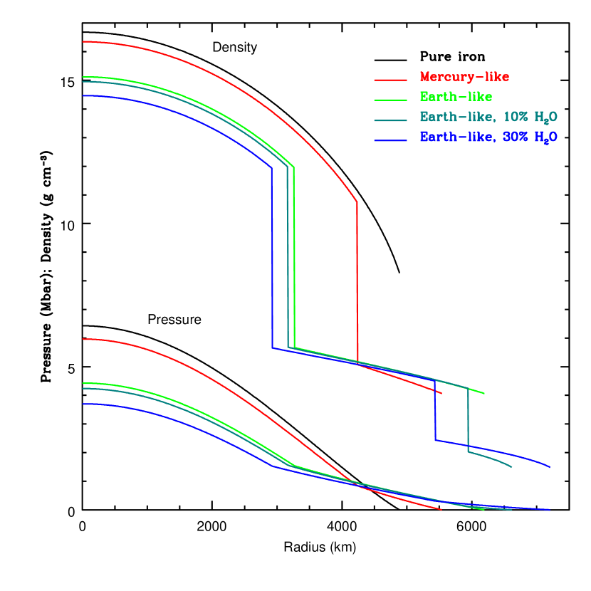
Figure 12.— Density and pressure profiles of various iron core/MgSiO₃ mantle planets, including two with deep water layers, all 1 M_⊕. “Earth-like” is defined as a 13:27 ratio of iron to MgSiO₃ mass, and “Mercury-like” is defined as 7:3 ratio of iron to MgSiO₃ mass, corresponding to the compositions of Earth and Mercury when water is not included. Planets with a greater core mass fraction have a smaller radius for a given mass due to the high density of iron relative to that of MgSiO₃.

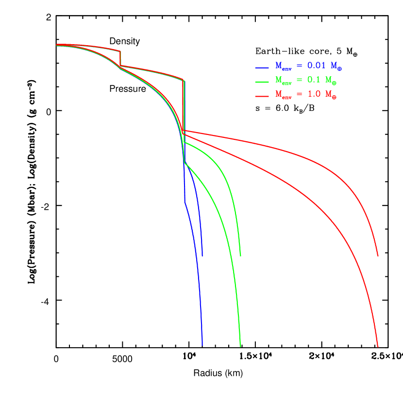
Figure 13.— Density and pressure profiles of planets with a 5-M_⊕ Earth-like core plus H₂-He envelopes equal to 0.01, 0.1, and 1.0 M_⊕. In each case, the envelope has a constant entropy of 6.0 $k_{B}/B$. Increasing the envelope mass compresses the core slightly, making the core radius smaller.

In this section, we provide several figures relating to the internal structures of the planets we model. Figure 12 shows pressure and density profiles of several representative solid planet models, each with a mass of 1 M_⊕. We include pure iron, Mercury-like, and Earth-like compositions, along with “water-worlds” that are otherwise Earth-like, but have 10% and 30% water (Ice VII). Similarly, Figure 13 shows pressure and density profiles of representative models with H₂-He envelopes. These models each have a core mass of 5 M_⊕ and entropy of 6.0 $k_{B}$ per baryon, and envelope masses of 0.01, 0.1, and 1.0 M_⊕ are plotted. Increasing the envelope mass slightly compresses the core, decreasing the core radius.

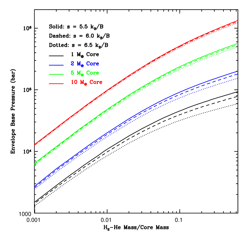
Figure 14.— Pressure at the base of the envelope versus envelope mass fraction for planets with constant core masses of 1, 2, 5, and 10 M_⊕. Curves with entropies of 5.5, 6.0, and 6.5 $k_{B}/B$ are plotted.

Figure 14 shows the base pressure of the envelope versus envelope mass fraction ($f_{env}$) for models with various constant core masses. For shallow envelopes for which the gravity does not vary significantly, the expected base pressure is

$$P_{b}\approx\frac{M_{env}g}{4\pi R^{2}}\approx\frac{GM_{c}M_{env}}{4\pi R^{4}}\approx\frac{GM_{c}^{2}f_{env}}{4\pi R^{4}},$$ (2)

where $g$ is the surface gravity. This relation holds well for small envelope mass fractions, but the pressure is lower than the relation would imply for envelope mass fractions $\gtrsim 3\%$ due to the variation in gravity over the height of the envelope.

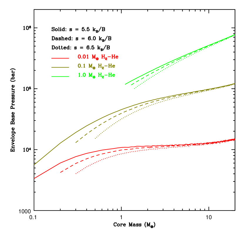
Figure 15.— Pressure at the base of the envelope versus core mass for planets with constant envelope masses of 0.01, 0.1, and 1.0 M_⊕. Curves with entropies of 5.5, 6.0, and 6.5 $k_{B}/B$ are plotted.

For low envelope fractions, the plot also shows a relation remarkably close to $P_{b}\propto M_{c}$. Figure 15 shows why this is so, plotting envelope base pressure versus core mass for constant envelope masses of 0.01, 0.1, and 1.0 M_⊕. The envelope base pressure in nearly constant over a wide range of core masses for shallow envelopes. Evidently, based on the relation above, $M_{c}/R^{4}$ is nearly constant for these models. This is supported by our power law fit for Earth-like solid planets of $R\propto M^{0.266-0.274}$ (see Section 7). On the other hand, if the core mass is low enough that the H₂-He comprises $\gtrsim$10% of the total mass, then the base pressure increases roughly linearly with core mass. Also, the entropy begins to have a significant effect on the base pressure in models with small cores, likely due to the increasing dependence of the radius on entropy as the core mass decreases (see Figure 4).

Figure 16.— Central pressure (top) and density (bottom) of planets with a 10-M_⊕ Earth-like core and a variable envelope mass. Entropies of 5.5, 6.0, and 6.5 $k_{B}/B$ are plotted. Despite a large change in total mass, the central pressure and density change very little.

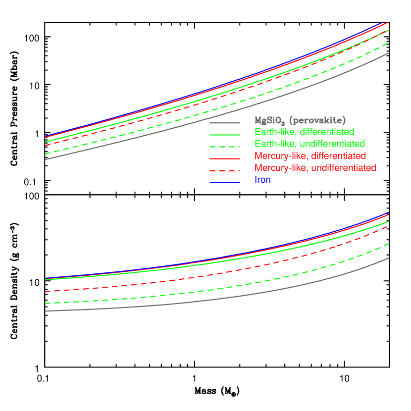
Figure 17.— Central pressure (top) and density (bottom) as a function of mass for constant-composition iron core/MgSiO₃ (perovskite) mantle planets in the 0.1$-$20 M_⊕ range. The iron mass fractions shown are 0%, 32.5% (Earth-like), 70% (Mercury-like) and 100%. Solid lines are differentiated, dashed lines are undifferentiated.

We also plot curves of central pressure and density versus envelope mass for models with a constant core mass of 10 M_⊕ and entropies of 5.5, 6.0, and 6.5 $k_{B}$ per baryon. Despite a large change in total mass, the central pressure and density change very little$-$about 5% in density and 10% in pressure for a doubling of total mass.

Central pressure and density versus (total) mass curves for representative solid planets, both differentiated and undifferentiated, are compared in Figure 17. The pure MgSiO₃ (perovskite) planet profile is included in order to demonstrate the discontinuity that arises in central density when a material of higher density is added. The planets with iron cores all have very similar central densities, while undifferentiated planets with varying iron fractions have lower central densities. This pattern repeats to a lesser degree for central pressures.

7. Solid Exoplanets

For completeness, we now provide mass-radius curves and tables for a range of solid exoplanet models with no significant envelopes. We construct true “terrestrial” planets with iron and MgSiO₃ components as well as three-component models with iron, MgSiO₃, and water, in the form of Ice VII, corresponding to “water worlds.” Figure 1 shows mass-radius plots for some of our representative solid planet models compared with masses and radii of observed exoplanets.

While we compute each curve from 0.1 to 20 M_⊕, our core-envelope decomposition results suggest that planets larger than $\sim$8 M_⊕ will likely have gaseous envelopes. Therefore our models of solid planets likely should only be applied to planets $\lesssim$8 M_⊕ that do not have extended envelopes. However, gaseous envelopes of close-orbiting planets could later be stripped away by evaporation by XUV irradiation, particularly for planets with initial masses $\lesssim$0.3 M_J orbiting young Solar-type stars (2007Icar..187..358H).

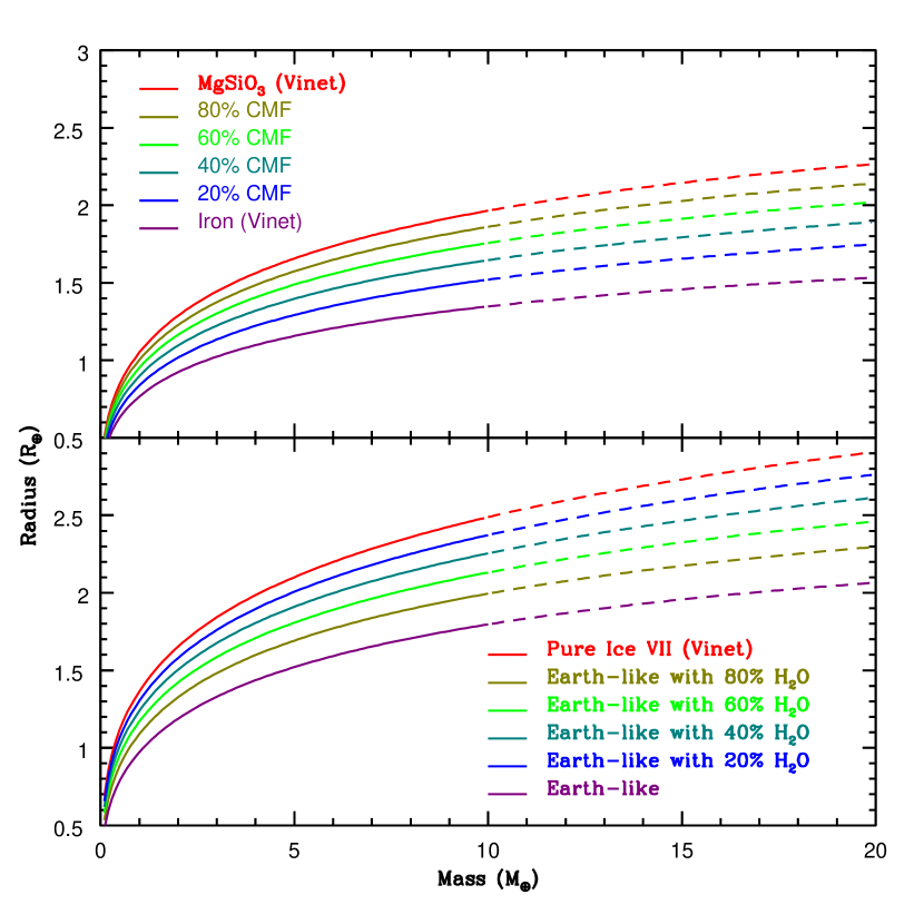
Figure 18.— Mass-radius curves for solid planets with various core mass fractions (CMF) ranging from 0% to 100%. Top panel: terrestrial models with iron cores and MgSiO₃ mantles. Bottom panel: “water worlds” with “cores” having an Earth-like structure plus a deep water layer (in the form of Ice VII).

In Figure 18, we plot terrestrial models with different iron core mass fractions (CMFs), ranging from pure iron to pure MgSiO₃ (perovskite), showing a systematic trend of decreasing radius with increasing CMF. We also plot models of “water worlds” with an Earth-like core (Earth-like in having the same Fe/Mg ratio as Earth), ranging from a purely Earth-like composition to pure water. Because the water worlds have some iron content, they overlap with terrestrial models with lower iron content, even given the lower density of water, pointing to a degeneracy with composition in the mass-radius plot. These results show good agreement with those of 2007ApJ...665.1413V, 2007Icar..191..337S, 2007ApJ...669.1279S, and 2007ApJ...659.1661F.

A power-law fit of the form $R\propto M^{x}$ provides a simple description of the behavior of the mass radius curves. 2006Icar..181..545V performed such a fit over the span of their “super-Earths” (1$-$10 Earth masses, 33% CMF) and “super-Mercurys” (1$-$10 Mercury masses, 70% CMF), and we compute the values of $x$ in our fits for comparison. For “super-Earths,” we find a power-law coefficient of 0.266$-$0.274, while 2006Icar..181..545V reported a range of 0.267$-$0.272. For “super-Mercurys,”, we find a power-law coefficient of 0.309$-$0.312, comparable to the “$\sim$0.3” reported by 2006Icar..181..545V. The lower masses of the “super-Mercurys” result in less compression in their interiors, and a power-law fit closer to the $R\propto M^{\frac{1}{3}}$ law for uncompressed planets than for super-Earths.

The super-Earths with currently observed masses and radii consistent with a purely solid composition have masses of $\sim 2-8$ M_⊕. While these numbers are loose, we can use them in conjunction with our models to study the relation between radius and composition. For example, in this $\sim 2-8$ M_⊕ range, the range of radii for pure iron models (the minimum radius for a given mass) is $\sim 0.9-1.3$ R_⊕, in contrast with the range for pure silicates (the maximum radius for terrestrial compositions), which have radii of $\sim 1.25-2.0$ R_⊕, and water-rich models, which are larger still. While there are significant degeneracies with composition among solid planets, this reiterates the usefulness of radius as a proxy for distinguishing solid exoplanets from those with gaseous envelopes, since known planets larger than 2 R_⊕ cannot be purely rock/iron and are likely to have such gaseous envelopes (2013arXiv1311.0329L; 2014ApJ...783L...6W; 2014ApJS..210...20M).

Properties of differentiated planet models with Earth-like and Mercury-like compositions are given in Tables 14 and 16, respectively. For comparison, we present properties of pure iron and pure silicate planets in Tables 13 and 18, respectively.

8. Conclusions

We have investigated a range of exoplanet models for various core masses, gaseous envelope masses, and envelope entropies, and compared them with mass and radius observations. Some of our representative modeled planet properties are tabulated in Tables 7-18 for a variety of planet compositions. We have explored models with both “Earth-like” rock-iron cores and ice cores to account for the possibility of the formation of planets with gaseous envelopes in both the warm and cold regions of their “solar” systems, and we have investigated the correction for the presence of a radiative atmosphere. We also considered varying silicate and water fractions for solid planets.

We have decomposed observed exoplanets into core mass and envelope mass components for both rock-iron cores and ice cores. Based on measured masses and radii, we find that the envelope mass, $M_{env}$, may vary over a wide range of values from zero to tens of percent of the total mass over a wide range of total masses, except that for the higher-mass “sub-Neptune” (or “mini-Neptune”) planets, a nonzero envelope mass is always required to fit a rock-iron core. Thus, planetary formation and evaporation models need to account for the very wide range of core masses and envelope masses derived.

In general, an ice core model requires a smaller envelope mass (and larger core mass) to fit the same mass-radius pair as an Earth-like core model, because of the larger radius of the core. Entropy also has a systematic effect on the core-envelope decomposition: an envelope with higher entropy is hotter and has a lower density, so that a smaller envelope mass is needed to fit the same mass-radius pair. The correction for the presence of a radiative atmosphere is also significant, reducing the envelope mass needed to fit the data by 30%-50% for large envelopes, and sometimes eliminating the need for a convective envelope entirely in the case of small atmosphere masses. Therefore, given these uncertainties, we have derived a range of possible core and envelope masses for known Neptune- and sub-Neptune-sized exoplanets.

While a few planets have large envelope mass fractions of $\sim 22\%-35\%$ (when corrected for the radiative atmosphere), as shown in Figure 11 and Table 2, most of the “sub-Neptune” planets that have been observed are dominated by their core masses (Figures 10 and 11); that is, the envelope comprises only a small fraction of the total mass. At the same time, for core masses of $M_{c}\gtrsim 5$ M_⊕, the planetary radius is very sensitive to the envelope mass and also to the entropy, so that the observed radius can serve as a proxy for the properties of the envelope, subject to the degeneracies of envelope mass, entropy, and the depth of the radiative atmosphere.

For solid planets up to 20 R_⊕, we find that only planets with radii $\lesssim 1.5-2.0$ R_⊕ can be purely terrestrial (iron core plus silicate mantle). Observationally, the largest planet that is consistent with our terrestrial models is Kepler-20b, with $M=8.7\pm 2.2$ M_⊕ and $R=1.91_{-0.21}^{+0.12}$ R_⊕. In a transitional regime of $\sim$1.75-2.8 R_⊕ (which may correspond with an observed break in the planetary occurence function, 2013ApJS..204...24B), the abundance of both water and H₂-He may be important, but the effect of the water fraction on the radius diminishes for larger planets.

Determining the composition and structure of solid planets from mass and radius observations is more ambiguous than for planets with gaseous envelopes due to significant degeneracies and uncertainties. There is overlap in radius with different iron fractions and water fractions over the mass range at which planets with potentially-solid compositions have been observed. Further research is needed to standardize equations of state for planetary models and reduce uncertainties.

There remains a degeneracy between composition and envelope entropy, and more detailed atmospheric and evolutionary models are needed to estimate the atmospheric entropy of exoplanets (to a precision of $\sim 0.1k_{B}/B$) in order to make more accurate determinations of their compositions and envelope/core mass partitions. On the observational side, more precise mass measurements are needed to better constrain core masses, as well as envelope masses in the case of smaller planets. More planet detections with overall better statistics are also needed to fully populate the mass-radius diagram and determine the distinct populations of planets (if any) in this regime.

Appendix A Radius Code Verification

Our computational procedure for deriving planet structural profiles and the corresponding mass-radius relationships is as follows: We begin with a guess of central pressure and integrate the equations of hydrostatic equilibrium out until the pressure is zero. For differentiated planets, we dictate a boundary mass for the core material, at which we switch to the equation of state for the new material, maintaining pressure continuity. Our code admits an arbitrary number of layers of different materials. Because it is impossible to know the total mass or radius before the integration is performed, we use an iterative Newton-Raphson scheme to produce a planet of specified mass.

For hydrogen-helium envelopes, we assume an adiabatic pressure and density profile by setting a constant entropy, usually at 5.5$-$6.5 $k_{B}$ per baryon. This is a good approximation for convective envelopes, but not for radiative atmospheres, with the caveat that highly irradiated planets may be radiative to significant depths (1996ApJ...459L..35G; 2000ApJ...534L..97B). The code also relies on extrapolations for pressures of less than 10 bars. (Pressures this low are not encountered in solid planets.)

We use a fourth-order Runge-Kutta scheme to solve the equations of hydrodynamic equilibrium:

$$\frac{dP}{dr}=-\frac{Gm\rho}{r^{2}}$$ (A1)

$$\frac{dm}{dr}=4\pi r^{2}\rho,$$ (A2)

where $r$ is the radius, $\rho$ is the mass density, $P(\rho)$ is the pressure given by the EOS, and $m$ is the mass interior to $r$. We use various radius step sizes ranging from 10$-$100m depending on the size of the planet model.

We test our code with the polytropic equation of state, $P=K\rho^{1+\frac{1}{n}}$ with $n=$1.5, 2, 2.5, and 3. Our results for the constants $\rho_{c}/\bar{\rho}$ (scaled density) and $\xi$ (scaled radius) agree with the values found in 1939isss.book.....C to a part in $10^{5}$.

Appendix B Equations of State

For solid planets, we implement two semi-empirical equations of state for most materials. The first is the third-order Birch-Murnagham EOS, given by

$$P_{3}=\frac{3}{2}K_{0}\left[x^{\frac{7}{3}}-x^{\frac{5}{3}}\right]\left\{1+\frac{3}{4}\left(K^{\prime}_{0}-4\right)\left[x^{\frac{2}{3}}-1\right]\right\},$$ (B1)

where $x$ is the ratio $\rho/\rho_{0}$, $\rho_{0}$ is the zero-pressure density, $K_{0}$ is the bulk modulus at $\rho=\rho_{0}$, and $K^{\prime}_{0}$ is the pressure derivative of the bulk modulus at $\rho=\rho_{0}$. Values for the second pressure derivative of the bulk modulus at $\rho=\rho_{0}$, $K^{\prime\prime}_{0}$, are in most cases not available, but for materials which have a known $K^{\prime\prime}_{0}$, a fourth-order term can be added to the third-order B-M EOS:

$$P_{4}= P_{3}+\frac{3}{2}K_{0}\left[x^{\frac{7}{3}}-x^{\frac{5}{3}}\right]\frac{3}{8}\left(x^{\frac{2}{3}}-1\right)^{2}$$ (B2)

$$\times\left[K_{0}K^{\prime\prime}_{0}+K^{\prime}_{0}\left(K^{\prime}_{0}-7\right)+\frac{143}{9}\right].$$

The second semi-empirical equation of state that we implement is the Vinet EOS, given by

$$P=3K_{0}x^{2/3}\left[1-x^{-\frac{1}{3}}\right]\exp{\left(\frac{3}{2}\left(K^{\prime}_{0}-1\right)\left[1-x^{-\frac{1}{3}}\right]\right)}.$$ (B3)

A summary of the equations of state used in our models is given in Table 5.

Table 5Equations of State Used for this Project^a

Material	EOS	$\rho_{0}$ (g cm-3)	K0 (Mbar)	K${}^{\prime}_{0}$	Ref
Fe ($\epsilon$)	Vinet	8.267	1.634	5.38	1
MgSiO3	Vinet	4.064	2.48	3.91	2
(perovskite)
MgO	B-M3	3.5833	1.602	3.99	3
(periclase)
SiC (ZB)b	B-M3	3.350	2.271	3.79	4
SiC (RS)b	B-M3	4.256	2.666	4.64	4
Diamond	Vinet	3.5171	4.45	4.0	5
Platinum	Vinet	21.46	2.70	5.64	6
H2O Ice VII	Vinet	1.4876	1.49	6.2	7
H2-He	Tabular				8

^aAll of the values are for materials at zero pressure and temperature. $\rho_{0}$ is the density, K₀ is the bulk modulus, and K${}^{\prime}_{0}$ is the pressure derivative of the bulk modulus.

^bThe SiC EOS with zincblende (ZB) structure is used for pressures up to 0.75 Mbar, beyond which the EOS with rock salt (RS) structure is used.

Which EOS fit is used for a given material makes little difference at low pressures where the zero-pressure density dominates. In Figure 19, models using the Vinet and B-M semi-empirical equations of state for pure MgSiO₃ (perovskite) are used to generate mass-radius curves, which differ by only 0.3% for 1 Earth-mass planets, 0.3% for 5 Earth-mass planets, and 1.2% for 10 Earth-mass planets. These results agree with those reported in 2007ApJ...669.1279S, who found that the mass-radius curves for low-mass exoplanets depend only on the uncompressed density. The differences become more significant for planets of higher mass (and, therefore, higher internal pressure), amounting to $\sim$3.3% for 20 Earth-mass silicate planets and 7.0% for 20 Earth-mass iron planets, although we do not expect to see solid planets of this size without H₂-He envelopes (2013arXiv1311.0329L; 2014ApJ...783L...6W). A more detailed summary of differences is given in Table 6.

Table 6Difference in Radius Between Planets with Vinet and B-M Equations of State

Mass (M⊕)	Pure Fe	Pure MgSiO3	Pure H2O
1.0	0.072%	-0.286%	0.239%
5.0	1.64%	0.251%	0.417%
10.0	3.58%	1.17%	1.06%
20.0	7.02%	3.27%	2.38%

To better illustrate the differences between the various equations of state, the pressure-density curves for various EOSs fits for Mg₂SiO₄ (olivine) and MgSiO₃ (perovskite) are plotted in Figure 20 over the run of pressures found in super-Earths of mass up to 20 Earth masses (without gaseous envelopes). The curves show significant divergence in pressure at high densities, particularly for the different Mg₂SiO₄ EOSs, but remarkable similarities between the two materials, demonstrating that for rocky material, the choice of equation of state is more important than the precise chemical composition. For this reason, we do not address phase transitions in the mantle. This similarity breaks down below $\sim$1 Mbar, however, where the uncompressed density dominates. Notably, the $<1$ Mbar range includes most of the mantle of a 1-$M_{\earth}$ Earth-like planet, so the choice of phase transitions and the choice of silicate material could have a significant effect for lower-mass planets.

For context, internal pressure and density profiles for model 1-M_⊕ planets of various compositions are plotted in Figure 12. 2000ipei.book.....P and 1996JPCM....8...67H report that the Vinet EOS is more suited to extrapolation to high pressures. However, as Table 1 demonstrates, a wide variety of EOS data and fits have been used in the literature. Unless otherwise specified, we use a Vinet EOS in building our models, but we also use a 3rd-Order B-M EOS in some cases, as indicated in Table 5. For H₂-He envelopes, we use the EOS of 1995ApJS...99..713S.

We do not employ thermal corrections in our model, but we can estimate their effect from the coefficients of thermal expansion. The volume thermal expansion coefficient at high pressures has been measured to be $2-3\times 10^{-5}$ K^-1 for iron (1990JGR....9521731B) and $4\times 10^{-5}$ K^-1 for MgSiO₃ (1986Natur.319..214K). Taking $3\times 10^{-5}$ K^-1 as an average, or a linear coefficient of $1\times 10^{-5}$ K^-1, and an internal temperature of 5,000 K, typical of Earth’s core (1994CRASB.318..341P), we can estimate a thermal correction to the planetary radius of about 5%. However, the internal temperature may be significantly higher for larger planets.

Alternatively, we can find the total error produced by our code from an Earth-analog model. Specifically a 1-M_⊕ planet model with an “Earth-like” composition produced by our code has a radius of 0.972 R_⊕, an error of 2.8%. This includes the error introduced by thermal expansion compared with our zero-temperature model, the errors in the equations of state, and the error introduced by the simplifying assumption of a two-layer model. Since the EOS-induced errors are small for a 1-M_⊕ planet, it is possible that thermal expansion is a significant contributor to this error.

We compare our mass-radius results for a simple iron core/MgSiO₃-mantle planet to those obtained by 2007ApJ...669.1279S, to determine the effect of any differences in the EOS. We test a pure MgSiO₃ composition, a 32.5% iron core mass fraction (CMF) (“Earth-like”) composition, a 70% CMF (“Mercury-like”) composition, and a pure iron composition for masses ranging from $0.5M_{\earth}$ to $20M_{\earth}$. We find agreement to within 1% in all cases, with the exception of pure iron planets, which differ by up to -2.23% for $20M_{\earth}$. This is likely due to the effect on the EOS of the higher central pressures of iron planets. Planets of mass 10 M_⊕ composed of pure iron, 70% iron, 32.5% iron, and pure MgSiO₃ (perovskite) have central pressures of 88 Mbar, 78 Mbar, 54 Mbar, and 18 Mbar, respectively.

As Figures 19 and 20 demonstrate, there can be slight differences between different EOS fits. Ambiguities are especially prominent in the 1 to 1000 Mbar pressure range, the latter being above pressures one can probe with constant-temperature experiments, but below where the Thomas-Fermi-Dirac EOS becomes applicable (1987Natur.330..737H). In order to investigate the effect of EOS ambiguities on a terrestrial planet model, we multiply the density for all pressures by a constant error factor. The resulting mass-radius curves for pure iron and pure silicate planets are given in Figure 21.

For a 10% swing in density at a given pressure (on the order of the differences between EOSs in Figure 20), we find changes in radius for pure MgSiO₃ planets of -3.5% (0.1 M_⊕), -4.0% (1.0 M_⊕), -4.6% (5.0 M_⊕), -5.0% (10.0 M_⊕), and -5.5% (20.0 M_⊕). For pure iron planets, we find changes of -3.7% (0.1 M_⊕), -4.4% (1.0 M_⊕), -5.0% (5.0 M_⊕), -5.3% (10.0 M_⊕), and -6.4% (20.0 M_⊕).

While most equations of state for a given material will agree on the low-pressure density (as it is easily measured), the differences between equations of state in the 1 to 1000 Mbar range could exceed 5%. Because of this, the ambiguities in radius we report are relevant to high-mass planets (without envelopes) and solid cores whose central pressures lie where the equation of state is ambiguous. In particular, the uncertainties in radius due to the equation of state are similar in magnitude to the change in radius caused by differentiation and different mantle material (e.g. silicates vs. silicon carbide), so more accurate equations of state are needed to distinguish these cases.

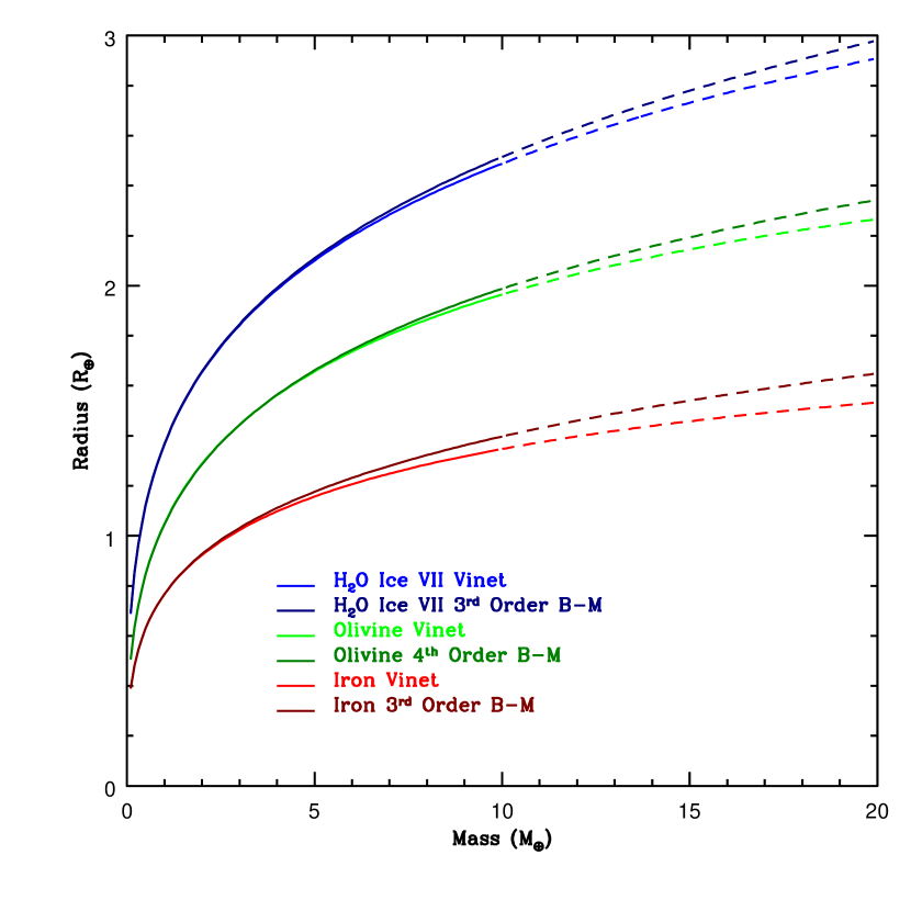
Figure 19.— Comparison of mass-radius curves computed with Vinet and Birch-Murnaghan EOSs for water (in the form of Ice VII), Mg₂SiO₄ (olivine), and iron. The two EOS fits agree in the low-pressure limit where the uncompressed density dominates, but deviate at high pressures. For context, the EOS fits for olivine differ by only 0.2% for 1 Earth-mass planets, but differ increasingly as planet mass increases (to 6.8% for 20 Earth-mass planets).

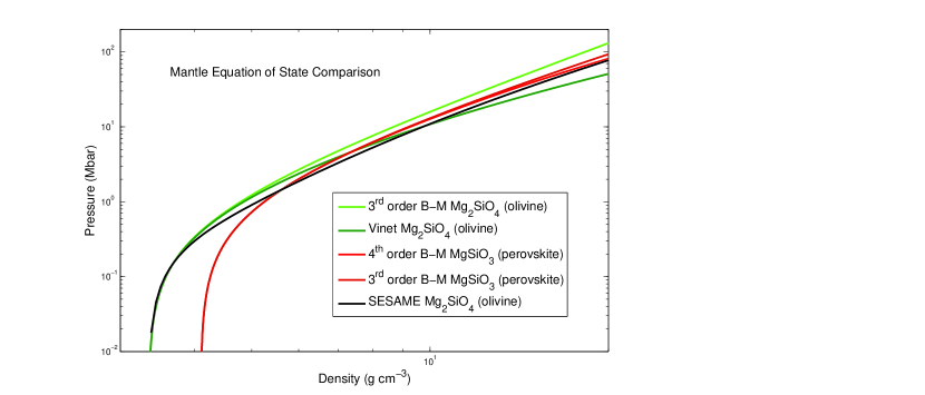
Figure 20.— Comparison of various equations of state for mantle materials. At high pressures ($>$1 Mbar) the equations of state for the two materials become similar, with the greatest differences between the various equations of state occurring for Mg₂SiO₄ (olivine). This implies that for mantle materials at high pressures, the choice of material has a less significant effect than the choice of EOS fit. However, at pressures approaching zero, the uncompressed density dominates, making the choice of material far more significant than the choice of EOS fit at low pressures.

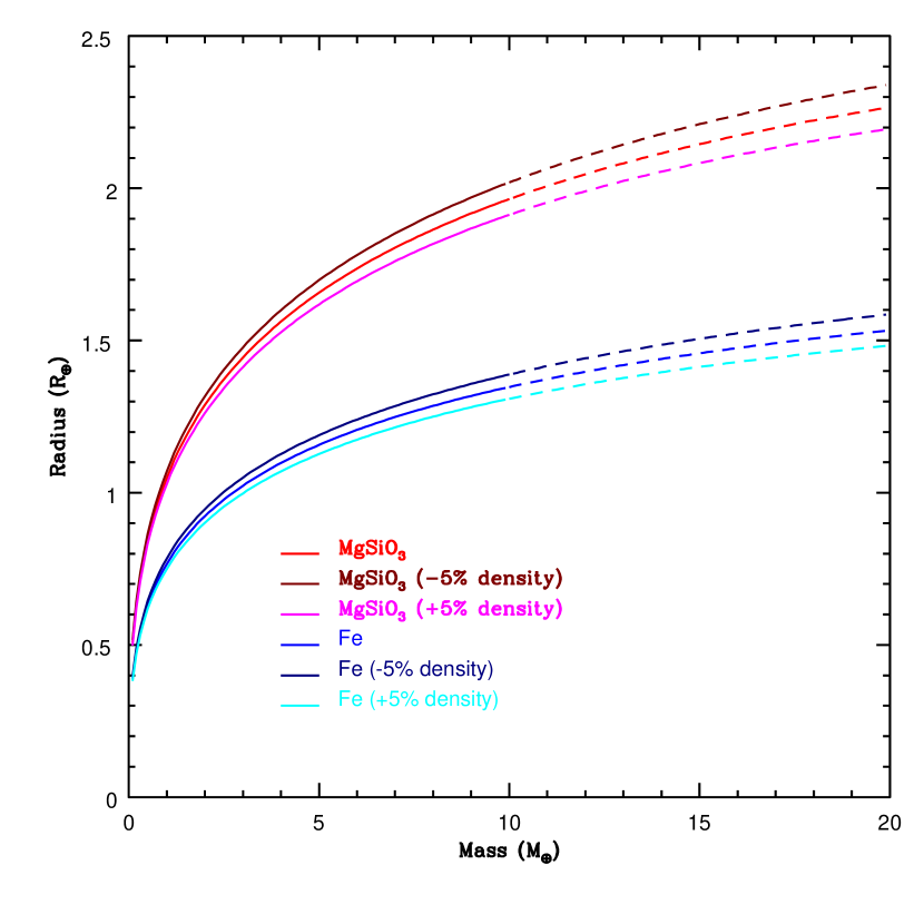
Figure 21.— Mass-radius curves for pure iron and silicate planets. A proportional EOS error in density is applied to investigate the effects of EOS ambiguities on terrestrial planet models. For a 10% swing in density at a given pressure, we find changes in radius ranging from -3.5% for a silicate, 0.1-M_⊕ planet to -6.4% for an iron, 20-M_⊕ planet.

Table 7Earth-Like Core/H₂-He Envelope Planets with $M_{env}=0.1$ M_⊕, $s=6.0\,k_{B}/B$

Core Mass	Radius	Central Pressure	Central Density
(M⊕)	(R⊕)	(Mbar)	(g cm-3)
0.4	4.26148	1.97466	12.5530
0.6	3.47101	2.28146	13.5698
0.8	3.06142	3.66167	14.4290
1	2.79890	4.50292	15.1893
2	2.33196	8.82066	18.2349
3	2.21482	13.3997	20.6751
4	2.17903	18.2692	22.8259
5	2.17231	23.4375	24.8049
6	2.17681	28.9078	26.6708
7	2.18852	34.6839	28.4580
8	2.20358	40.7688	30.1884
9	2.21951	47.1661	31.8770
10	2.23497	53.1950	33.5349
12	2.26575	69.0382	36.7901
14	2.29493	84.0288	40.0016
16	2.32147	101.173	43.2015
18	2.34494	119.786	46.4135
20	2.36655	139.946	49.6562

Table 8Earth-Like Core/H₂-He Envelope Planets with $M_{c}=2$ M_⊕, $s=5.5\,k_{B}/B$

Envelope Mass	Radius	Central Pressure	Central Density
(M⊕)	(R⊕)	(Mbar)	(g cm-3)
0.00	1.18851	8.69496	18.1594
0.02	1.56409	8.73952	18.1862
0.04	1.73518	8.76965	18.2044
0.06	1.87084	8.79355	18.2187
0.08	1.99033	8.81374	18.2308
0.10	2.09529	8.83109	18.2412
0.20	2.52114	8.89454	18.2790
0.30	2.84728	8.93799	18.3049
0.40	3.11830	8.97101	18.3245
0.50	3.35079	8.99829	18.3407
0.60	3.55310	9.02147	18.3544
0.70	3.73529	9.04193	18.3665
0.80	3.89788	9.06027	18.3773
0.90	4.04563	9.07698	18.3872
1.00	4.18264	9.09255	18.3963
1.20	4.42436	9.12031	18.4127
1.40	4.63533	9.14551	18.4275
1.60	4.82146	9.16841	18.4409
1.80	4.98358	9.18966	18.4534

Table 9Earth-Like Core/H₂-He Envelope Planets with $M_{c}=2$ M_⊕, $s=6.0\,k_{B}/B$

Envelope Mass	Radius	Central Pressure	Central Density
(M⊕)	(R⊕)	(Mbar)	(g cm-3)
0.00	1.18851	8.69496	18.1594
0.02	1.67729	8.73677	18.1846
0.04	1.88652	8.76455	18.2013
0.06	1.97443	8.78670	18.2146
0.08	2.20039	8.80485	18.2255
0.10	2.33232	8.82073	18.2350
0.20	2.85687	8.87792	18.2691
0.30	3.25957	8.91662	18.2922
0.40	3.59448	8.94581	18.3095
0.50	3.87978	8.97001	18.3239
0.60	4.12971	8.99055	18.3361
0.70	4.34681	9.00852	18.3467
0.80	4.54684	9.04297	18.3565
0.90	4.72604	9.03955	18.3651
1.00	4.89030	9.05350	18.3733
1.20	5.17685	9.07834	18.3880
1.40	5.42263	9.10066	18.4011
1.60	5.63461	9.12127	18.4132
1.80	5.82015	9.14026	18.4244

Table 10Earth-Like Core/H₂-He Envelope Planets with $M_{c}=2$ M_⊕, $s=6.5\,k_{B}/B$

Envelope Mass	Radius	Central Pressure	Central Density
(M⊕)	(R⊕)	(Mbar)	(g cm-3)
0.00	1.18851	8.69496	18.1594
0.02	1.84538	8.73323	18.1825
0.04	2.12095	8.75821	18.1975
0.06	2.34125	8.77764	18.2092
0.08	2.53227	8.79358	18.2187
0.10	2.70473	8.80722	18.2269
0.20	3.40678	8.85628	18.2562
0.30	3.94117	8.88858	18.2755
0.40	4.38415	8.91308	18.2901
0.50	4.76993	8.93324	18.3021
0.60	5.10259	8.95047	18.3123
0.70	5.39890	8.96549	18.3212
0.80	5.66089	8.97905	18.3293
0.90	5.89601	8.99134	18.3366
1.00	6.10857	9.00277	18.3422
1.20	6.47809	9.02340	18.3555
1.40	6.78834	9.04236	18.3667

Table 11Earth-Like Core/H₂-He Envelope Planets with $M_{c}=5$ M_⊕, $s=6.0\,k_{B}/B$

Envelope Mass	Radius	Central Pressure	Central Density
(M⊕)	(R⊕)	(Mbar)	(g cm-3)
0.00	1.52092	23.2071	24.7228
0.02	1.80841	23.2701	24.7445
0.04	1.92515	23.3202	24.7626
0.06	2.01793	23.3631	24.7781
0.08	2.09911	23.4022	24.7922
0.10	2.17720	23.4374	24.8049
0.20	2.47107	23.5808	24.8565
0.30	2.70888	23.6902	24.8957
0.40	2.91421	23.7796	24.9277
0.50	3.09611	23.8562	24.9550
0.60	3.26045	23.9224	24.9786
0.70	3.41082	23.9813	24.9996
0.80	3.55018	24.0346	25.0186
0.90	3.67956	24.0840	25.0361
1.00	3.80286	24.1288	25.0520
1.20	4.02328	24.2093	25.0806
1.40	4.22312	24.2808	25.1059
1.60	4.40458	24.3449	25.1285
1.80	4.57070	24.4041	25.1495
2.00	4.72406	24.4582	25.1685
2.50	5.06239	24.5797	25.2113
3.00	5.34830	24.6854	25.2484
3.50	5.59620	24.7809	25.2819
4.00	5.83033	24.8764	25.3153
4.50	6.00929	24.9518	25.3416

Table 12Earth-Like Core/H₂-He Envelope Planets with $M_{c}=10$ M_⊕, $s=6.0\,k_{B}/B$

Envelope Mass	Radius	Central Pressure	Central Density
(M⊕)	(R⊕)	(Mbar)	(g cm-3)
0.00	1.79615	53.5130	33.4467
0.02	1.99228	53.6051	33.4688
0.04	2.07032	53.6835	33.4876
0.06	2.13342	53.7542	33.5046
0.08	2.18642	53.8190	33.5201
0.10	2.23596	53.8813	33.5350
0.20	2.43488	54.1477	33.5987
0.30	2.59648	54.3693	33.6515
0.40	2.73667	54.5604	33.6971
0.50	2.86268	54.7313	33.7377
0.60	2.97828	54.8846	33.7741
0.70	3.08500	55.0238	33.8071
0.80	3.18559	55.1530	33.8377
0.90	3.28040	55.2727	33.8660
1.00	3.36982	55.3828	33.8920
1.20	3.53525	55.5862	33.9400
1.40	3.69025	55.7704	33.9834
1.60	3.83086	55.9349	34.0222
1.80	3.96291	56.0866	34.0578
2.00	4.08644	56.2271	34.0908
2.50	4.36723	56.5416	34.1644
3.00	4.61361	56.8150	34.2283
3.50	4.83412	57.0578	34.2850
4.00	5.03420	57.2804	34.3368
4.50	5.21535	57.4825	34.3837
5.00	5.38451	57.6730	34.4279
6.00	5.68357	58.0220	34.5087
7.00	5.94431	58.3358	34.5811
8.00	6.17595	58.6298	34.6488

Table 13Pure MgSiO₃ (perovskite) Planets

Mass	Radius	Central Pressure	Central Density
(M⊕)	(R⊕)	(Mbar)	(g cm-3)
0.2	0.634704	0.44969	4.66933
0.4	0.791132	0.76609	5.00284
0.6	0.897857	1.06129	5.27594
0.8	0.980917	1.34800	5.51649
1	1.04968	1.63112	5.73586
2	1.28797	3.05157	6.66347
3	1.44433	4.53165	7.45104
4	1.56222	6.09528	8.17135
5	1.65714	7.75175	8.85318
6	1.73659	9.50646	9.51142
7	1.80482	11.3635	10.1551
8	1.86449	13.3270	10.7901
9	1.91740	15.4003	11.4208
10	1.96480	17.5872	12.0502
12	2.04659	22.3176	13.3149
14	2.11495	27.5538	14.5999
16	2.17308	33.3339	15.9166
18	2.22312	39.7017	17.2748
20	2.26653	46.7077	18.6833

Table 1432.5% Iron / 67.5% MgSiO₃ (perovskite) Differentiated Planets

Mass	Radius	Central Pressure	Central Density
(M⊕)	(R⊕)	(Mbar)	(g cm-3)
0.2	0.592384	1.08997	11.2072
0.4	0.736224	1.94664	12.5157
0.6	0.833926	2.77697	13.5207
0.8	0.909741	3.60223	14.3719
1.0	0.972372	4.43009	15.1266
2	1.18850	8.69494	18.1594
3	1.32962	13.2340	20.5953
4	1.43571	18.0696	22.7440
5	1.52093	23.2070	24.7217
6	1.59214	28.6485	26.5866
7	1.65321	34.3970	28.3729
8	1.70657	40.4541	30.1021
9	1.75383	46.8249	31.7898
10	1.79616	53.5130	33.4467
12	1.86914	67.8618	36.6994
14	1.93012	83.5511	39.9084
16	1.98200	100.637	43.1054
18	2.02670	119.191	46.3144
20	2.06553	139.285	49.5533

Table 1532.5% Iron / 67.5% MgSiO₃ (perovskite) Undifferentiated Planets

Mass	Radius	Central Pressure	Central Density
(M⊕)	(R⊕)	(Mbar)	(g cm-3)
0.2	0.593662	0.596268	5.82786
0.4	0.737793	1.03360	6.33721
0.6	0.835511	1.44955	6.75061
0.8	0.911201	1.85902	7.11316
1	0.973627	2.26762	7.44304
2	1.18822	4.36307	8.83494
3	1.32751	6.60057	10.0176
4	1.43167	9.00490	11.1022
5	1.51499	11.5858	12.1321
6	1.58431	14.3501	13.1295
7	1.64351	17.3037	14.1081
8	1.69501	20.4523	15.0765
9	1.74045	23.8027	16.0411
10	1.78097	27.3617	17.0068
12	1.85037	35.1346	18.9558
14	1.90784	43.8386	20.9471
16	1.95624	53.5474	22.9986
18	1.99745	64.3474	25.1257
20	2.03281	76.3381	27.3427

Table 1670% Iron / 30% MgSiO₃ (perovskite) Differentiated Planets

Mass	Radius	Central Pressure	Central Density
(M⊕)	(R⊕)	(Mbar)	(g cm-3)
0.2	0.535687	1.39506	11.7182
0.4	0.662772	2.54306	13.2557
0.6	0.748595	3.67582	14.4425
0.8	0.814977	4.81495	15.4518
1	0.869685	5.96775	16.3500
2	1.05786	12.0087	19.9881
3	1.18039	18.5516	22.9409
4	1.27243	25.6011	25.5667
5	1.34640	33.1514	27.9993
6	1.40823	41.2004	30.3062
7	1.46131	49.7471	32.5268
8	1.50776	58.7933	34.6864
9	1.54895	68.3429	36.8026
10	1.58589	78.4005	38.8879
12	1.64978	100.070	43.0034
14	1.70339	123.870	47.0883
16	1.74922	149.882	51.1807
18	1.78893	178.211	55.3085
20	1.82366	208.966	59.4937

Table 1770% Iron / 30% MgSiO₃ (perovskite) Undifferentiated Planets

Mass	Radius	Central Pressure	Central Density
(M⊕)	(R⊕)	(Mbar)	(g cm-3)
0.2	0.537303	0.914989	8.15393
0.4	0.664291	1.63148	9.06921
0.6	0.749565	2.33087	9.79947
0.8	0.815181	3.03122	10.4338
1	0.869019	3.73887	11.0074
2	1.05228	7.45597	13.4028
3	1.16984	11.5200	15.4184
4	1.25710	15.9491	17.2568
5	1.32649	20.7482	18.9951
6	1.38396	25.9242	20.6731
7	1.43288	31.4829	22.3140
8	1.47531	37.4317	23.9330
9	1.51264	43.7801	25.5410
10	1.54585	50.5397	27.1464
12	1.60261	65.3367	30.3725
14	1.64946	81.9292	33.6493
16	1.68884	100.440	37.0047
18	1.72233	121.008	40.4615
20	1.75106	143.796	44.0398

Table 18Pure Iron Planets

Mass	Radius	Central Pressure	Central Density
(M⊕)	(R⊕)	(Mbar)	(g cm-3)
0.2	0.481284	1.47742	11.8462
0.4	0.591383	2.71052	13.4467
0.6	0.664753	3.93539	14.6857
0.8	0.720967	5.17286	15.7419
1	0.766975	6.42967	16.6836
2	0.923092	13.0654	20.5136
3	1.02317	20.3131	23.6389
4	1.09763	28.1668	26.4291
5	1.15705	36.6171	29.0228
6	1.20647	45.6585	31.4895
7	1.24872	55.2906	33.8702
8	1.28555	65.5144	36.1910
9	1.31813	76.3373	38.4707
10	1.34727	87.7620	40.7217
12	1.39751	112.461	45.1776
14	1.43952	139.698	49.6177
16	1.47532	169.583	54.0822
18	1.50626	202.237	58.6007
20	1.53329	237.809	63.1980