Deterministically Driven Avalanche Models of Solar Flares

Abstract

We develop and discuss the properties of a new class of lattice-based avalanche models of solar flares. These models are readily amenable to a relatively unambiguous physical interpretation in terms of slow twisting of a coronal loop. They share similarities with other avalanche models, such as the classical stick–slip self-organized critical model of earthquakes, in that they are driven globally by a fully deterministic energy loading process. The model design leads to a systematic deficit of small scale avalanches. In some portions of model space, mid-size and large avalanching behavior is scale-free, being characterized by event size distributions that have the form of power-laws with index values, which, in some parameter regimes, compare favorably to those inferred from solar EUV and X-ray flare data. For models using conservative or near-conservative redistribution rules, a population of large, quasiperiodic avalanches can also appear. Although without direct counterparts in the observational global statistics of flare energy release, this latter behavior may be relevant to recurrent flaring in individual coronal loops. This class of models could provide a basis for the prediction of large solar flares.

1 Reconnection Avalanches and Parker’s Nanoflare Hypothesis

Identifying the physical mechanism responsible for coronal heating is still standing as one of the grand challenges of contemporary solar physics (see Klimchuk, 2006; Aschwanden et al., 2007; De Pontieu et al., 2011, for different theoretical and observational viewpoints). Nearly a quarter of a century ago, Parker (1983b) began exploring in earnest the possibility that coronal heating could be due to thermal energy released by small magnetic reconnection events occurring continuously throughout the magnetized corona (see Parker, 1983a, 1988; Priest, Heyvaerts, and Title, 2002, and references therein for related physical scenarii). His physical picture for nanoflare production is now well-known. Photospheric fluid motions associated with turbulent convection randomly shuffle the magnetic footpoints of coronal loop leading to a braiding of fieldlines throughout the volume of the loop, with which is associated an inexorable buildup of current sheets, as individual fieldlines try to return to dynamical equilibrium under the topological constraints imposed by flux-freezing. As these localized current systems build up, plasma instabilities eventually set in and lead to energy release through magnetic reconnection. Parker dubbed these elementary energy release events “nanoflares”, went on to argue that they occur continuously throughout the corona, and conjectured that they are responsible for coronal heating.

Intense efforts have been expended to observationally verify or contradict Parker’s conjecture. This is no easy task, as it involves measuring the energy output of flares very close to the detection limit of the best current solar imagers in space. On the other hand, decades of flare observations have shown that the probability distribution function [$f(E)$] for flare energy [$E$] takes the form of a power law [$f(E)\propto E^{-\alpha}$] spanning some eight orders of magnitude in energy, with $\alpha$ estimated in the range $1.65$ – $1.95$ (e.g. Aschwanden et al., 2000; Aschwanden and Charbonneau, 2002; Aschwanden, 2011, and references therein). This is too low for small flares to dominate energy input into the corona (requiring $\alpha>2$), unless the PDF steepens abruptly below the current detection limit. This is possible but increasingly unlikely as instruments such as the EUV imagers on the Transition Region And Coronal Explorer (TRACE) and Solar Dynamics Observatory (SDO) have pushed the detection limit right up to the boundary of the nanoflare regime. Another possibility is that physical models used to infer thermal energy release from EUV or soft X-ray fluxes are in error, due to erroneous assumptions regarding the intrinsic geometry of the flaring volume (McIntosh and Charbonneau, 2001), or of the physical conditions therein, required to infer thermal energy release from observed radiative fluxes (see McIntosh, 2000; Aschwanden and Parnell, 2002; Aschwanden, Zhang, and Liu, 2013, and references therein).

Whatever recent observational determination of $f(E)$ may imply for coronal heating, Parker’s scenario certainly remains a fine model for solar flares in general. Although not originally emphasized by Parker, his nanoflare scenario contains all ingredients now understood to be required to lead to self-organized criticality (hereafter SOC; see, e.g. Bak, Tang, and Wiesenfeld, 1987; Jensen, 1998): an open dissipative system – here a coronal loop – slowly driven – here by random footpoint motions – and subjected to a self-limiting local threshold instability – here magnetic reconnection. Despite the slow and gradual loading of energy, such a physical system will release energy in an intermittent manner, in the form of avalanches that can span up to the whole system.

Lu and Hamilton (1991) have proposed an avalanche-type model for solar flares that has become a reference model in the solar context, although numerous variations have now been developed over the intervening years. The present article describes one such variation that (we believe) is particularly interesting in that i) it is readily amenable to (relatively) unambiguous physical interpretation in terms of twisting of a coronal loop, and ii) it can yields qualitatively distinct flaring behavior as the degree of conservation is allowed to vary. Section sec:newmod briefly describes the original Lu and Hamilton model (more specifically, the version put forth by Lu et al., 1993, hereafter the “LH model”), along with the various manners in which we have altered the forcing and redistribution rules. Section sec:results provides modelling results, comparing and contrasting the statistical properties of avalanches in the LH model and our variations thereof. We conclude in Section sec:conclusion with a discussion comparing and contrasting our models with other classes of globally and deterministically driven avalanches models developed in different physical contexts, outlining some possible model improvements, and by summarizing the implications of our modelling results for coronal heating (and more specifically with regards to the flaring behavior of small coronal loops) as well as solar flares predictions.

2 A Class of Avalanche Models With Deterministic Driving

sec:newmod

2.1 The Lu and Hamilton Model ssec:LH

Following in part Kadanoff et al. (1989), Lu and Hamilton (1991) developed a SOC avalanche model for solar flares that by now has become a kind of “standard” (for a review, see Charbonneau et al., 2001). The original Lu and Hamilton model is a cellular automaton defined over a 3D regular cartesian grid with nearest neighbour connectivity (top+down+right+left+front+back) over which a vector field [${\mathbfit A}$] is defined. Here we will consider instead a 2D version of the model, where a scalar nodal quantity [$A_{i,j}^{n}$] is defined over the lattice. Robinson (1994) has shown that for the type of driving used in the Lu and Hamilton model, the use of a vector nodal variable yields results identical (statistically) to the use of a scalar variable. Also, strictly speaking the term “cellular automaton” should be restricted to lattice models where the nodal variable is discrete (i.e. integers mapping to a finite number of possible nodal states); in cases where the nodal variable is continuous, one is dealing with a “coupled map lattice”. We retain “cellular automaton” here, because it has become common usage in this context. The superscript $n$ is a discrete time index, and the subscript pair [$i,j$] identifies a single node on the 2D lattice. Keeping $A=0$ on the lattice boundaries, the cellular automaton is driven by adding one small increment in $A$ per time step, at some randomly selected node that changes from one time step to the next. A deterministic stability criterion is defined in terms of the local curvature of the field at node $(i,j)$:

$$\ilabel{eq:stab1}\Delta A_{i,j}^{n}\equiv A^{n}_{i,j}-\frac{1}{4}\sum_{k}A_{k}^{n}\,,$$ (1)

where the sum runs over the four nearest neighbours at nodes $(i,j\pm 1)$ and $(i\pm 1,j)$. If this quantity exceeds some pre-set threshold [$Z_{c}$] then an amount of nodal variable [$Z$] is redistributed to the same four nearest neighbours according to the following discrete, deterministic rules:

$$\ilabel{eq:redis1}A_{i,j}^{n+1}=A_{i,j}^{n}-\frac{4}{5}Z~{},$$ (2)

$$\ilabel{eq:redis2}A_{i\pm 1,j\pm 1}^{n+1}=A_{i\pm 1,j\pm 1}^{n}+\frac{1}{5}Z~{},$$ (3)

with $Z=\rm{sign}(\Delta A)Z_{c}$. Following this redistribution, it is possible that one of the nearest neighbour nodes now exceeds the stability threshold. The redistribution process begins anew from this node, and so on in classical avalanching manner. Driving is suspended during avalanching, implicitly implying a separation of timescales between driving and avalanching dynamics, and all nodal values are updated synchronously during an avalanche to avoid introducing a directional bias in avalanche propagation.

It is readily shown that these redistribution rules, while conservative in $A$, lead to a decrease in $A^{2}$ summed over the five nodes involved by an amount

$$\ilabel{eq:erel1}\Delta e_{i,j}^{n}=\frac{4}{5}\left(2{\left|\Delta A_{i,j}^{n}\right|\over Z_{c}}-1\right)Z_{c}^{2}~{},$$ (4)

with the energy released being “assigned” to the unstable node $(i,j)$. If one identifies $A^{2}$ with a measure of magnetic energy (more on this shortly), the total energy liberated by all unstable node at a given iteration is then equated to the energy release per unit time in the flare:

$$\ilabel{eq:elatt}(\Delta E)^{n}=\sum_{\rm unstable}\Delta e_{i,j}^{n}~{}.$$ (5)

A natural energy unit here, used in all that follows, is the quantity of energy [$e_{0}$] liberated by a single node exceeding the stability threshold by an infinitesimal amount; setting $|\Delta A_{i,j}|\approx Z_{c}$ in Equation (eq:erel1) immediately leads to

$$\ilabel{eq:eunit}e_{0}=(4/5)Z_{c}^{2}~{}.$$ (6)

This very simple model yields a strikingly good representation of flare statistics, namely the observed power law form (and associated exponents) of the frequency distributions of flare peak energy release [$P$], duration [$T$], and total energy release (see Lu and Hamilton, 1991; Charbonneau et al., 2001; Aschwanden and Charbonneau, 2002). However, Equations (eq:stab1) – (eq:redis2) are admittedly very far removed from the MHD equations governing the process of magnetic reconnection, but there exist plausible bridges across this conceptual chasm.

2.2 Physical Interpretationssec:phys

We adopt here a variation (Charbonneau, 2013) of the interpretative picture originally put forth by LH. The 2D lattice will be considered as a slice across a coronal loop, i.e. in cylindrical coordinates $(\varpi,\phi,z)$ (see schematic in Figure fig:schematic_global_forcingA), a slice in the $\varpi\phi$-plane, with the loop axis in the $z$-direction, and the lattice variable as the $z$-component of the magnetic vector potential ${\mathbfit A}$ such that ${\mathbfit B}=\nabla\times{\mathbfit A}$. Such a magnetic field automatically satisfies the solenoidal constraint $\nabla\cdot{\mathbfit B}=0$. The vector potential component [$A_{z}$] then defines the magnetic field component in the $\varpi\phi$-plane, which can be directly related to the degree of twist in the loop, i.e. the ratio of transversal to longitudinal field components. As argued by LH, adding small random increments of $A$ at one lattice node then corresponds to adding a small amount of twist somewhere in the loop, which fits nicely the Parker scenario outlined above. Moreover, the stability criterion becomes a threshold condition on $\nabla^{2}(A_{z}\hat{{\mathbfit z}})$, i.e. the magnitude of the longitudinal component of the electric current, which is also satisfying from the point of view of MHD stability.

This ansatz suffers from one significant difficulty, however: there is not necessarily a one-to-one correspondence between the squared nodal variable (squared vector potential) and magnetic energy as conventionally defined [$\propto\int B^{2}{\rm d}V$]. It was nevertheless shown (see Figure 12.6 in Charbonneau, 2013) that the correspondance of $A^{2}$ to $B^{2}$ is empirically almost always satisfied, in the sense that the variations of $A^{2}$ almost always follow the variations of $B^{2}$ in our model.

2.3 Deterministic Global Drivingssec:detdrive

The Parker picture of random shuffling of a loop’s magnetic footpoint by photospheric flows makes sense if the loop is of diameter comparable to (or preferably larger) than the granular length scale, and if no larger fluid motions co-exist near the base of the loop. The granular or larger scale flow otherwise displaces the footpoints in a spatially coherent manner far removed from random shuffling. One particularly interesting form of such global forcing is a twisting of the loop’s footpoints (illustrated in Figure fig:schematic_global_forcing), which then propagates upwards and accumulates along the length of the loop [$A\rightarrow B$]. Such a twisted magnetic loop can become unstable (e.g. to a kink-type instability, $B\rightarrow C$, see Baty and Heyvaerts, 1996; Bareford, Browning, and van der Linden, 2010, and references therein). Local tangential discontinuities arise and associated current sheets appear. Magnetic reconnections release energy locally and reduce the effective stresses [$C\rightarrow D$], possibly restoring the loop stability [$D\rightarrow E$]. Note also that the final stable state [$E$] is not necessarily twist-free; it is generally composed of a particular pattern of stresses resulting from the past reconnection history in the loop.

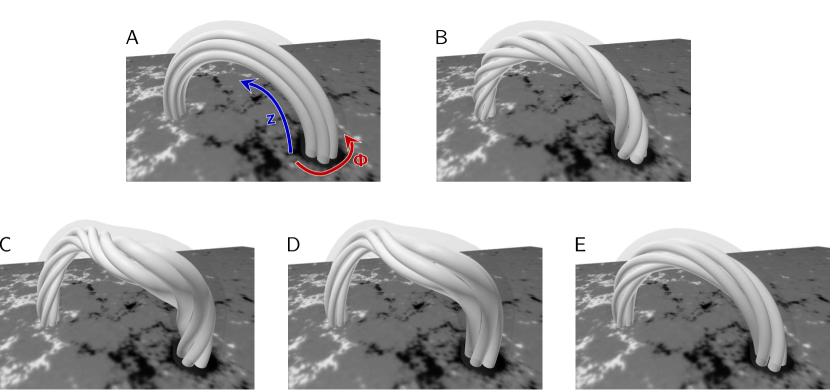
Figure 1.: Cartoon of a physical interpretation of the deterministic forcing and its associated avalanches in the context of a solar coronal loop. See text for a detailed description.fig:schematic_global_forcing

This form of global forcing and energy release mechanism has a direct equivalent in our 2D cellular automaton. Working in cylindrical coordinates $(\varpi,\phi,z)$, with the loop axis in the $z$-direction, the total magnetic field can be written as

$$\ilabel{eq:bdef}{\mathbfit B}(\varpi,\phi,t)=\nabla\times(A_{z}(\varpi,\phi,t){\hat{\mathbfit z}})+B_{z}(\varpi){\hat{\mathbfit z}}~{}.$$ (7)

Identifying now the nodal variable $A$ with $A_{z}$ sampled on the lattice, consider the following deterministic, global driving mechanism:

$$\ilabel{eq:detdrive}A_{i,j}^{n+1}=A_{i,j}^{n}\times(1+\varepsilon)~{},\qquad 0<\varepsilon\ll 1~{},\qquad\forall\,(i,j)~{},$$ (8)

where the parameter $\varepsilon$ ($\ll 1$) is a measure of the driving rate. With $A_{z}=0$ on the boundaries, the SOC state is peaked at the center of the lattice, and far enough from the latticed boundaries is characterized by near-axisymmetry about the lattice center. This implies that $\nabla\times(A_{z}{\hat{{\mathbfit z}}})$ is primarily in the $\phi$-direction. The above driving mechanism thus amounts to a geometrical increase of $B_{\phi}$ by a factor $(1+\varepsilon)^{n}$ after $n$ driving iterations, while $B_{z}$ remains unaffected. In other words, the degree of twist within the loop increases geometrically as well. The stability criterion based on the magnitude of the longitudinal component of the electric current then becomes a natural criterion on the intensity of the current sheet(s) developing in the loop.

In addition, $B_{\phi}$ is increasing in direct proportion to $A_{z}$ everywhere in the loop, which means that associating $A^{2}$ summed over the lattice with magnetic energy is entirely realistic in this context. All avalanche models discussed in the remainder of this article make use of this global, deterministic driving scheme. As in the LH model, driving is interrupted during avalanching, which amounts to assuming that the driving timescale is much longer than the avalanching timescale, a reasonable assumption in the solar coronal context (for a discussion, see Lu, 1995).

Similar global, deterministic driving schemes have been used extensively in the context of SOC models of seismic faults, based on a cellular automaton representation of the Burridge–Knopoff stick–slip model (see Olami, Feder, and Christensen, 1992; Lise and Paczuski, 2001, and references therein). The main difference from our model resides in their stability criterion that applies to the nodal variable rather than, in our case, to its curvature. A global, deterministic driver has also been used by Liu et al. (2006); Vallières-Nollet et al. (2010); Liu et al. (2011) in their cellular automaton model of magnetospheric substorms generation in the Earth’s central plasma sheet. To our knowledge, Hamon, Nicodemi, and Jensen (2002) have been the only authors to explore deterministically driven avalanche models in the context of solar flares. They used a slightly modified version of the original model of Olami, Feder, and Christensen (1992), in which the threshold triggering the avalanching behavior applies is defined on the nodal variable rather than its curvature. In the present study, we use the latter criterion, which is naturally inherited from the original LH model.

Evidently, the form of deterministic driving embodied in Equation (eq:detdrive) precludes using the initial condition $A_{i,j}^{0}=0$. In what follows we typically use a lattice having reached the SOC state via the original LH model, and then switch to deterministic driving. This will typically lead to a transient phase during which the lattice reajusts to the new driving scheme, and/or other altered model components, as discussed presently. This transient phase is usually accompanied by a gradual change in the total lattice energy, so that monitoring the latter is the best way to ascertain the recovery to a statistically stationary avalanching state.

2.4 Stochastic Redistribution Rulesssec:storedst

Directly incorporating the deterministic driving rule given by Equation (eq:detdrive) within the Lu and Hamilton model yields a deterministic cellular automaton characterized by a periodic cycle of energy loading/unloading, all energy release events having the same magnitude. To recover SOC-like behavior, some stochastic element need be reintroduced somewhere in the model.

2.4.1 Random Redistributionsssec:rr

Consider the following, plausible stochastic variation on the Lu and Hamilton redistribution rules: the same amount of nodal variable [$Z$] is always removed from any unstable site, following the Lu et al. (1993) prescription, but it is distributed randomly, rather than equally, amongst its four nearest neighbours:

eq:redis3$$A_{i,j}^{n+1} = A_{i,j}^{n}-\frac{4}{5}Z~{},$$ (9)

eq:redis4$$A_{i\pm 1,j\pm 1}^{n+1} = A_{i\pm 1,j\pm 1}^{n}+{4\over 5}\left({r_{k}\over R}\right)Z~{},$$ (10)

where the $r_{k}$ ($k=1,...,4)$ are random deviates uniformly distributed in $[0,1]$, and $R=\sum r_{k}$. This scheme will be referred to as random redistribution. Note that here that some particular random sequences and node configurations may lead to negative energy release from the redistribution process. We avoid such unphysical events by permuting the four random numbers over the neighbouring nodes and then sometimes generate four new random numbers until a positive energy is released by the avalanche.

2.4.2 Random Extractionsssec:re

Another means of introducing stochasticity is to retain equal redistribution to nearest neighbours, but let the quantity $Z$ extracted from the unstable node be drawn from a bounded distribution of uniform random deviates

$$\ilabel{eq:redis5}Z\in[|\Delta A_{i,j}^{n}|-Z_{c},Z_{c}]~{},$$ (11)

while retaining Equations (eq:redis1) – (eq:redis2) for the redistribution per se. The lower bound in Equation (eq:redis5) ensures that the redistribution will, at worst, restore marginal stability, while the upper bound corresponds to the setting of the Lu and Hamilton model. This scheme will be referred to as random extraction, and, defined in the above manner, involves no adjustable parameters once $Z_{c}$ has been specified.

2.4.3 Nonconservative Redistributionsssec:nc

A third approach is to introduce non-conservative redistribution rules. In all rules discussed so far – including the original Lu and Hamilton rules – redistribution is conservative, in that whatever quantity of $A$ being extracted from an unstable node ends up in the nearest neighbours, whether in equal (Equations (eq:redis1) – (eq:redis2)) or unequal (Equations (eq:redis3) – (eq:redis4)) proportions. This conservation property is basically inspired by the sandpile analogy, where avalanches redistribute sand grains without creating or destroying any. With a nodal variable associated with a single component of the magnetic vector potential, there exist no physical requirement for conservative redistribution of $A$; the important physical requirement, namely $\nabla\cdot{\mathbfit B}=0$, is already taken care of under the current interpretive scheme, see Equation (eq:bdef).

A nonconservative version of the Lu and Hamilton redistribution rules can be defined as follows:

$$\ilabel{eq:redis8}A_{i,j}^{n+1}=A_{i,j}^{n}-\frac{4}{5}\,Z~{},$$ (12)

$$\ilabel{eq:redis9}A_{i\pm 1,j\pm 1}^{n+1}=A_{i\pm 1,j\pm 1}^{n}+{r_{0}\over 5}Z~{},$$ (13)

where $r_{0}\in[D_{\rm nc},1]$ is again extracted from a uniform distribution of random deviates with a lower bound [$D_{\rm nc}$ ($<1$)], such that $1-D_{\rm nc}$ is the fraction of the redistributed quantity $Z$ that is lost rather than redistributed. This rule thus involves one free parameter, namely the conservation parameter [$D_{\rm nc}\in[0,1[$]. A nonconservative model of this type, using fully deterministic driving, redistribution, and stability criteria, has been developed by Liu et al. (2006); Vallières-Nollet et al. (2010) in the context of magnetospheric substorms, and has been shown to produce avalanches with SOC-like power-law distribution for event sizes.

2.5 Stochastic Thresholdssec:stothresh

Another interesting possibility is to introduce stochasticity at the level of the stability threshold. This can be achieved, for example, by replacing the deterministic threshold rule given by Equation (eq:stab1) by extracting a value $Z_{c}$ anew at each node of each temporal iteration from a sharply peaked normal distribution centered on some mean value ${\bar{Z}_{c}}$. An important parameter in such a scheme is the width at half-maximum [$\sigma$] of the Gaussian distribution; if $\sigma$ is very small (in the sense that $\sigma/{\bar{Z}_{c}}\ll 1$, one expects behavior similar to the conventional, fixed threshold stability rule, while a very wide Gaussian turns the stability threshold into a random triggering process driven by noise.

Lu et al. (1993) experimented with similar random variations of the threshold rules in the context of their stochastically driven model, but report no significant variations of the results as compared to their deterministic threshold rule. As will become apparent further below, in the context of a deterministically driven model, however, interesting effects are produced in the regime $\sigma/{\bar{Z}_{c}}\ll 1$.

To sum up, we are displacing the stochastic element in the Lu and Hamilton model from the forcing rule to either the redistribution rule or the threshold rule. In the original Lu and Hamilton model, avalanche dynamics is fully deterministic but the driving is stochastic. The model variations outline above move the stochastic element to the avalanche dynamics, in the context of a spatially global and fully deterministic driving mechanism that can be interpreted plausibly as global twisting of a coronal loop.

3 Resultssec:results

In principle, fully deterministic avalanche models, e.g. the LH model with the deterministic driving defined by Equation (eq:detdrive) and a smooth initial condition, lead to a regular cycle of energy loading/unloading, with avalanches equally spaced in time and all liberating the same amount of energy. The challenge in reintroducing stochasticity in the stability and/or redistribution rules is to break this deterministic loading/unloading cycle (in this context, see also Wheatland and Glukhov, 1998, and references therein).

In the preceding section we have introduced various classes of redistribution rules based on a number of stochastic elements, as well as a stochastic threshold rule. A large number of distinct avalanche models can be constructed by picking and combining this or that model element. One could, for instance, build a fixed-threshold model using nonconservative redistribution rules (Section sssec:nc) with equal distribution to nearest neighbors; or a conservative rule with random distribution to nearest-neighbors (Section sssec:rr), in conjunction with a stochastic threshold rule (Section ssec:stothresh). In addition, each such model may involve adjustable parameters (e.g. the width [$\sigma$] of the Gaussian distribution from which the threshold values are extracted). Although we have explored a vast portion of the relevant model space, in what follows we focus on a relatively small subset of such models, chosen so as to illustrate the range of behaviours possible in deterministically driven avalanche models. In order to expedite this exploration of parameter space, most model runs were carried out on a small grid ($48^{2}$), but we have also recomputed a number of runs on larger grids (up to $384^{2}$) to ensure that the results reported upon below are robust with respect to lattice size.

Exploration of model space quickly reveals that an important behavioral discriminant is the conservative property (or lack thereof) of the redistribution rule. Consequently we first discuss results for a variety of conservative models (Section ssec:rescons), and turn subsequently to their non-conservative counterparts (Section ssec:resncons). We finally considers (Section ssec:fss) the origin of the break of finite size scaling that takes place in our models.

3.1 Conservative Redistributionssec:rescons

Table tab:cons lists the defining rules and parameter values of a set of representative conservative avalanche models, whose properties will be discussed in the remainder of this section. Here and in all that follows, unless noted otherwise all models are run on a $48^{2}$ lattice, use the driving scheme described by Equation (eq:detdrive), and a stability threshold $Z_{c}=1$ (or ${\bar{Z}_{c}}=1$ for models with a stochastic threshold). A “0” entry in the second column indicates a deterministic threshold rule. The entry “random” in the third and fourth columns indicates use of Equations (eq:redis5) and (eq:redis3) – (eq:redis4), respectively. The last line in the Table lists the “ingredients” of the LH model, for comparison.

	$\sigma/Z_{c}$	Extraction	Redistribution	$\alpha_{E}$	$\alpha_{P}$	$\alpha_{T}$
C1	0.0	Random	$4\times 1/5$	$1.43\pm 0.044$	$1.49\pm 0.243$	$1.94\pm 0.136$
C2	0.01	$Z_{c}$	$4\times 1/5$	$1.47\pm 0.008$	$1.84\pm 0.019$	$1.92\pm 0.023$
C3	0.0	$Z_{c}$	Random	$1.29\pm 0.026$	$1.42\pm 0.045$	$1.38\pm 0.022$
C4	0.01	Random	$4\times 1/5$	$1.40\pm 0.013$	$1.56\pm 0.087$	$1.77\pm 0.033$
C5	0.01	$Z_{c}$	Random	$1.29\pm 0.015$	$1.47\pm 0.037$	$1.38\pm 0.011$
C6	0.0	Random	Random	$1.22\pm 0.009$	$1.12\pm 0.037$	$1.47\pm 0.008$
C7	0.01	Random	Random	$1.19\pm 0.015$	$1.08\pm 0.034$	$1.42\pm 0.004$
LH	0.0	$Z_{c}$	$4\times 1/5$	$1.48\pm 0.005$	$1.72\pm 0.143$	$1.63\pm 0.023$

Table 1.: Conservative avalanche models, with a driving parameter $\varepsilon=10^{-6}$. Error bars were obtained with ten different random number sequences.tab:cons

Figure fig:tscons shows a short segment of the time series for total lattice energy (a) and energy release (b) in model C3. This is a model using deterministic extraction, random redistribution, a fixed stability threshold $Z_{c}$, and a deterministic driving parameter $\varepsilon=10^{-6}$. The lattice energy time series exhibits a pattern of quasiperiodic energy loading and unloading. As can be seen in Figure fig:tsconsb, the unloading takes place via a sequence of large avalanches of roughly similar amplitudes and durations taking place at more or less regular time intervals. Comparison between panels c and a reveals that a small but significant fraction ($\lesssim 1\%$) of the total lattice energy is dissipated by any one of these large avalanches, in between which lattice energy grows almost steadily in response to driving. Careful scrutiny of Figure fig:tsconsb also reveals a population of much smaller avalanches interspersed between these large ones. Figure fig:tsconsd is a zoom with an expanded vertical scale, spanning an interval between two large avalanches and showing the smaller ones in better detail. Unlike the quasiperiodic large avalanches, these are seen to span a wide range of amplitudes, and show no hint of any (quasi)periodicities. Even the largest avalanches in this second population only release a minuscule fraction of the lattice energy, and are hardly visible during the energy loading rising phases in Figure fig:tsconsa.

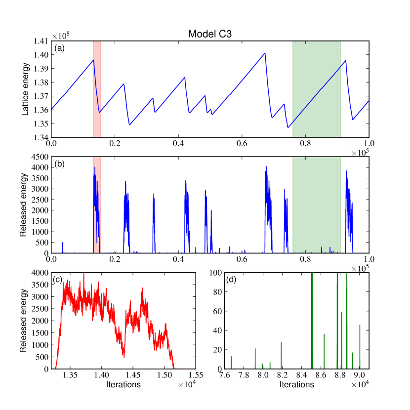
Figure 2.: Sample time series for avalanche model C3. (a) Temporal evolution of total lattice energy. (b) Energy released by avalanches. There are two populations of avalanches here: quasiperiodic large avalanches (c), in between which occurs a population of smaller avalanches spanning a wide range of scales in size (d). Energy is measured in the elementary unit $e_{0}$ given by Equation (eq:eunit).fig:tscons

All of this suggests the presence of (at least) two dynamically distinct avalanche populations. This impression is confirmed upon computing the probability distribution functions (hereafter PDF) for total energy release, i.e. the probability of finding an avalanche having released a total energy within the interval $[E,E+{\rm d}E]$. This PDF, as well as the corresponding PDF for peak energy release [$P$] and avalanche duration [$T$], are shown on Figure fig:pdfcons for a set of models. The bulk part of all three PDFs is well fitted by a power-law for all models, except at the high ends of the distributions. A marked excess of large, long duration events shows up as a bump – well fitted by a Gaussian –, and for cases with random redistribution/extraction a significant depletion for very low avalanches occurs (a detailed discussion on to this particular population is given at the end of this section). It is readily verified that the bump at the lower end of the PDF corresponds to the large avalanches, while the power-law portion of the PDF is made up of all avalanches taking place in between, as in Figure fig:tsconsd.

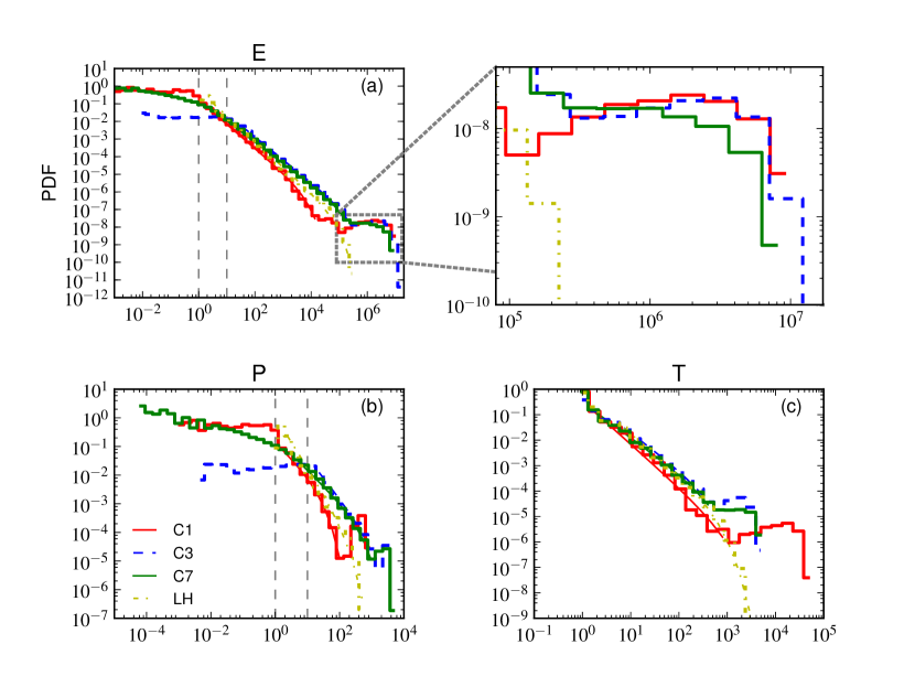
Figure 3.: Statistical properties of avalanches in models C1, C3, C7, and LH, as labeled. The various panels show the probability distribution functions of (a) total energy released by avalanches [$E$], (b) peak energy release [$P$], and (c) duration [$T$]. A close-up of the high-$E$ end of the total energy PDF is also shown. The straight lines are guides to the eye, showing the slopes associated with the mid-sized avalanches of the distributions. All PDFs are constructed from $10^{8}$ iterations runs, initialized from prior runs of the same models having already reached a statistically stationary state. The vertical dashed lines label the transition from small to power-law avalanches (see discussion a the end of section sec:results).fig:pdfcons

Evidently, in the case of model C3, the stochasticity introduced at the level of redistribution is insufficient to break the quasiperiodic pattern of energy loading and unloading, as manifested by the population of large avalanches. Indeed, this pattern proves surprisingly difficult to break. Figure fig:3ts shows $10^{5}$ iterations segments of energy release time series extracted from a sequence of three avalanche models, all operating at the same deterministic driving rate $\varepsilon=10^{-6}$, but including more and more stochastic components (specifically, models C3, C6, and C7 in Table tab:cons). Comparing the three panels reveals immediately that increasing stochasticity gradually breaks the quasiperiodicity of large avalanches, while blurring the energy contrast between the populations of large and small avalanches, mostly by reducing the size of the large loading/unloading avalanches. Corresponding PDFs for the integrated energy release [$E$], peak energy release [$P$] and avalanche duration [$T$] are also shown on Figure fig:pdfcons. Even in the case of the strongly stochastic model C7, these PDFs (solid green histograms in Figure fig:pdfcons) still show an excess of large events as compared to a pure, scale-free power-law distribution.

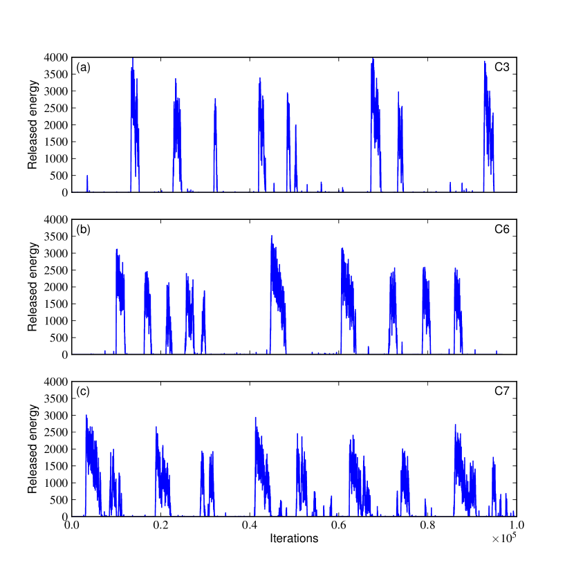
Figure 4.: Extracts of energy release time series in models C3, C6, and C7 (panels a through c). This represents a sequence of increasing stochasticity built into the avalanche models (cf. Table tab:cons). All models use the same deterministic driving rate, namely $\varepsilon=10^{-6}$ in Equation (eq:detdrive).fig:3ts

Further insight into this dichotomy in avalanching behavior is obtained by computing a waiting time distribution (WTD) separately for each class of avalanches. The waiting time [$\Delta T$] associated with the $k{\rm th}$ avalanche is defined as the time elapsed since the end of the previous avalanche and the beginning of that under consideration. The distinction between “large” and “small” avalanches is made on the basis of the PDF for peak energy release, which typically shows most clearly the bump associated with the population of large avalanches; as the PDF is scanned from the low end of the size distribution towards the high end, a point is reached where the PDF shows a local minimum (e.g. at $P/e_{0}\approx 2\times 10^{2}$ for model C1 in Figure fig:pdfconsb). All avalanches located right of this point are considered to belong to the population of “large” avalanches, even though they likely contain a few of the largest avalanches belonging to the second population of “small” avalanches, but there is simply no way to reliably distinguish these.

The WTDs for large and small avalanches are plotted in Figure fig:wtdconsa – b, here for C1-type models with driving rates $\varepsilon=10^{-7}$, $10^{-6}$, and $10^{-5}$. Large avalanches have a well-defined mean wait time and their WTD is well fitted by a Gaussian, while the population of smaller avalanches has an exponential WTD, indicative of triggering by a stationary random process. Increasing the driving reduces the mean wait time for large avalanches in direct proportion, while steepening the exponential WTD for the population of small avalanches. This indicates that the large avalanches are the (perturbed) signature of the energy loading/unloading process that would otherwise characterize a fully deterministic model. For the population of small avalanches, increasing the driving rate merely steepens the WTD while maintaining its exponential form. This is the same behavior observed in the LH model when the mean amplitude of the spatially random increments remains constant in time and space (on the WTD in the LH model, see also Norman et al., 2001; Wheatland, 2000).

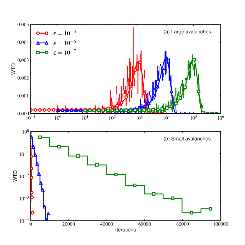
Figure 5.: Waiting-time distributions for the populations of (a) large and (b) small avalanches, for three C1-type models with deterministic driving rates of $\varepsilon=10^{-7}$, $10^{-6}$, and $10^{-5}$, as labeled. The WTDs for large avalanches are well fitted with a Gaussian (solid lines on panel a), while those characterizing small avalanches have an exponential form.fig:wtdcons

This is confirmed upon constructing scatter plots between the energy of large avalanches and the wait time elapsed since the end of the previous large avalanche, as done on Figure fig:Ewtd, for a sequence of C1-type models spanning four decades in driving rates: $\varepsilon=10^{-7}$, $10^{-6}$, and $10^{-5}$. For a simple, fully deterministic load/unload model (e.g. of the type originally considered by Rosner and Vaiana, 1978), avalanches are periodic and all liberate the same amount of energy; all points would then coincide. For a loading/unloading model including a stochastic trigger, one would expect a strong positive correlation between avalanche energy and wait time. For the spatially extended models considered here, individual avalanches are scattered in a cloud, whose extent in the $[E,\Delta T]$ plane increases with increasing degree of stochasticity in the avalanche model. This occurs because the unfolding of a large energy-unloading avalanche is affected by the spatial distribution of nodal variable values, itself influenced by the stochastic components introduced in the redistribution or threshold rules. Nonetheless, linear proportionality between energy and wait time is clearly apparent for the higher driving rates, but degrades towards lower $\varepsilon$-values; the linear correlation coefficients are $r=0.98$, $0.91$, and $0.89$ for $\varepsilon$ falling from $10^{-5}$ to $10^{-7}$, in decadal steps (see Figure fig:Ewtd).

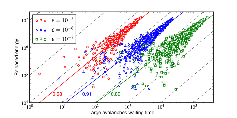
Figure 6.: Correlation between the energy of large avalanches, and the waiting time elapsed since the end of the previous large avalanche. Scatter plots are shown for C1-type models with varying driving rates [$\varepsilon$], as indicated. The dashed lines are a guide to the eye corresponding to a logarithmic slope of unity, indicating linear proportionality between avalanche energy and wait time, as expected in simple energy loading/unloading models (see text).fig:Ewtd

The models embedding a stochastic process in their redistribution or in their extraction rule (see Table tab:cons) all exhibit a particular population of small avalanches that is not well-fitted by a power-law (e.g. Figure fig:pdfconsa – b). These avalanches have an energy of the order of and lower than the unit energy [$e_{0}$]. In the case of the LH model, one-iteration – and one-node – avalanches always release an energy of $e_{0}$ whereas in the case of random redistribution or extraction, such avalanches can release a large range of different energies. This population of small avalanches – of few iterations – appears to deviate from the classical SOC state of the LH model. They can be easily identified in Fig. fig:E_vs_T where we scatter avalanches as a function of their duration [$T$] and released energy [$E$] for model C1. The alteration of very small avalanches can be different from one model to the other: model C1 shows a deviation for $E<e_{0}$ while model C3 is affected up to $E\approx 10\,e_{0}$. Despite the existence of scale-dependent populations at both ends of the avalanche distribution, the total energies of mid-size avalanches are still very well fitted by a power-law over more than four orders of magnitudes (more than two orders of magnitude for the peak energy).

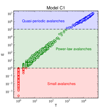
Figure 7.: [$E$] vs [$T$] in model C1. The three populations of avalanches (small, mid-size power law and large quasi-periodic) are well identified in three energy regions. fig:E_vs_T

The last three columns of Table tab:cons list the power-law indices obtained from least-square fits to the portions of the PDFs of total energy, peak energy release, and duration for the populations of mid-size avalanches in the corresponding simulations (the error bars were obtained with 10 runs using different random numbers sequences). These power-law indices are rather similar to those extracted from the 2D scalar version of the LH stochastically driven avalanche model (last line in Table tab:cons). Significant differences are observed nonetheless in going from model to model, suggesting that global statistics of event sizes are dependent to some extent on model “ingredients” and parameters in these conservative models.

We have explored a wide variety of conservative models, often combining into the same model multiple stochastic elements (see models C1 through C7 in Table tab:cons). Remarkably, none of these models succeeds in completely breaking the loading/unloading cycle. While producing scale-free avalanche size distributions spanning many decades in energy, all models also end up producing a population of very large quasi-periodic events with a more-or-less well-defined mean size. Even model C7, combining a fairly broad random stability threshold, random extraction, and random redistribution, ends up doing so. This property is truly robust, and holds over a wide range of driving rates. In contrast, the PDFs for flare sizes reconstructed from solar UV or soft X-ray data shows no such population, and is instead well represented by a single power-law (see Dennis, 1985; Lu et al., 1993; Aschwanden et al., 2000; Aschwanden and Parnell, 2002, and references therein). As detailed in what immediately follows, the use of nonconservative redistribution rules can alleviate this problem over a certain range in parameter space, for all classes of deterministically driven models.

3.2 Nonconservative Redistributionssec:resncons

We consider once again a representative set of deterministically driven avalanche model using non-conservative redistribution, as described in Section sssec:nc, and various combination of other modeling ingredients. Table tab:ncons lists the characteristics and properties of the models that are the focus of the foregoing discussion. The general format is similar to Table tab:cons, and the models were run with a non-conservation parameter $D_{nc}=0.1$. Recall that the actual fraction removed is drawn from a sequence of uniform deviates spanning $[D_{nc},1]$, so that the average nodal dissipation is the median of this interval. We essentially discuss in this section model NC0, the other models follow naturally the properties described in this and previous sections.

	$\sigma/Z_{c}$	Extraction	Redistribution	$\alpha_{E}$	$\alpha_{P}$	$\alpha_{T}$
NC0	0.0	$Z_{c}$	$4\times 1/5$	$1.17\pm 0.005$	$1.25\pm 0.097$	$1.15\pm 0.015$
NC1	0.0	Random	$4\times 1/5$	$1.12\pm 0.015$	$1.08\pm 0.037$	$1.22\pm 0.007$
NC2	0.01	$Z_{c}$	$4\times 1/5$	$1.20\pm 0.015$	$1.23\pm 0.080$	$1.16\pm 0.066$
NC3	0.0	$Z_{c}$	Random	$1.19\pm 0.007$	$1.25\pm 0.116$	$1.15\pm 0.009$
NC4	0.01	Random	$4\times 1/5$	$1.12\pm 0.014$	$1.04\pm 0.042$	$1.31\pm 0.098$
NC5	0.01	$Z_{c}$	Random	$1.21\pm 0.026$	$1.19\pm 0.025$	$1.19\pm 0.022$
NC6	0.0	Random	Random	$1.12\pm 0.021$	$1.08\pm 0.036$	$1.22\pm 0.010$
NC7	0.01	Random	Random	$1.12\pm 0.015$	$1.03\pm 0.023$	$1.29\pm 0.037$

Table 2.: Non-conservative avalanche models [$\varepsilon=10^{-6}$, $D_{\rm nc}=0.1$]. Error bars were obtained with ten different random-number sequences.tab:ncons

Figure fig:tsncons, similar in format to Figure fig:tscons, shows a $10^{6}$ iterations segment of the time series for total lattice energy (a) and energy release (b) in model NC0. This is now a nonconservative model using a driving rate $\varepsilon=10^{-6}$, fixed threshold and extraction, and equal redistribution to nearest-neighbors. The only stochasticity introduced here is at the level of non-conservation, with a random fraction between 0 and 90% of the nodal variable value being lost from each unstable node during redistribution. Comparing to Figure fig:tsconsa and b, one immediately notices the absence of the very large quasi-periodic avalanches characterizing models with conservative redistribution. The lattice-energy time series now has the fractal-sawtooth form characteristic of the original stochastically driven LH model. The largest avalanches still only release a small fraction of the total lattice energy (here about one percent at most, but much less on larger lattices). The peak energy release of avalanches now spans over three orders of magnitude even on the small $48^{2}$ lattice used here, indicating that the larger avalanches span the whole lattice. No hint of periodicities can be detected. These features suggest a SOC-like state with a scale-free distribution of avalanche sizes.

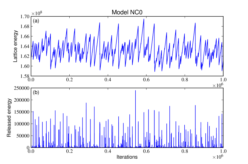
Figure 8.: Sample time series for avalanche model NC0 ($D_{nc}=0.1$). Panel (a) shows the temporal evolution of total lattice energy, and part (b) the energy released by avalanches. There is now a single population of avalanches, without a characteristic event size or quasiperiodicity in event occurrence.fig:tsncons

This impression is reinforced upon computing the PDFs for the size of avalanches. Unless the conservation parameter [$D$] tends towards unity (more about this shortly), these PDFs now take the form of pure power laws for mid-size and large avalanches (cf. Figure fig:pdfncons). Small avalanches appear to systematically depart from a power law distribution in a similar fashion to than observed for conservative models in Section ssec:rescons. The origin of the flattening is in fact the same: small avalanches have now the possibility to release energies in a much broader range than in the original LH model. This feature notwithstanding, at small conservation parameter all of these nonconservative models show a scale-free distribution for mid-size and large avalanches in total avalanche energy, peak energy release and duration.

Models with moderate to high conservation ($D_{\rm nc}\to 1$) do exhibit deviations from power-law behavior for the largest events. The limit $D_{\rm nc}\to 1$ takes us back to conservative models, so it is not surprising to see a second population of avalanches appear. Figure fig:pdfncons, shows a set of PDFs computed for a set of NC0-type model runs with driving rate fixed at $\varepsilon=10^{-6}$ and decreasing values of the dissipation parameter $D_{\rm nc}$, as labeled. Recall (Table tab:ncons) that except for the dissipation mechanism, these models are otherwise fully deterministic. The models at $D_{\rm nc}=0.1$ yield pure power laws, but at $D_{\rm nc}=0.5$ an excess of large events becomes apparent, which becomes quite pronounced at $D_{\rm nc}=0.99$.

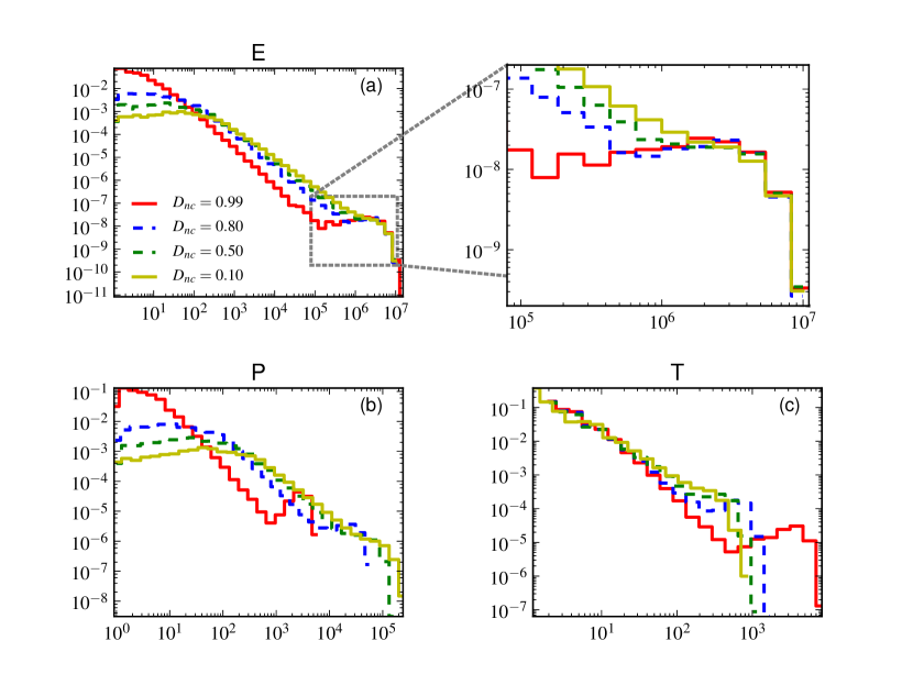
Figure 9.: Probability distribution functions of total avalanche energy in a set of NC0-type model runs with fixed driving rate $\varepsilon=10^{-6}$ but decreasing conservation parameter $D_{\rm nc}$, as labeled. The layout is similar to Figure fig:pdfcons: panel a, b and c show respectively $E$, $T$ and $P$.fig:pdfncons

Figure fig:alphancons shows how the power-law indices for (a) avalanche energy, (b) peak release, and (c) duration vary with driving rate [$\varepsilon$] and conservation parameter [$D_{nc}$], in the suite of NC0-type models runs. Each curve corresponds to a specific driving rate [$\varepsilon$], as labeled. The power-law indexes show little to no dependance to the driving rate – provided it is sufficiently low –, as expected. The general trend, namely steepening of the PDFs with conservation parameter, also characterizes the other types of nonconservative models listed in Table tab:ncons. A systematic dependence of the power-law indices with the conservation parameter is observed in Figure fig:alphancons. We fit the power law indices [$\alpha$] as a function of a power law of $D_{nc}$ (gray lines in Figure fig:alphancons) and obtain:

eq:fit_alphas$$\alpha_{E} = 1.18+\left(\frac{D_{\rm nc}}{2.48}\right)^{1.60}\,,$$ (14)

$$\alpha_{P} = 1.20+\left(\frac{D_{\rm nc}}{1.34}\right)^{2.00}\,,$$ (15)

$$\alpha_{T} = 1.15+\left(\frac{D_{\rm nc}}{1.35}\right)^{2.12}\,.$$ (16)

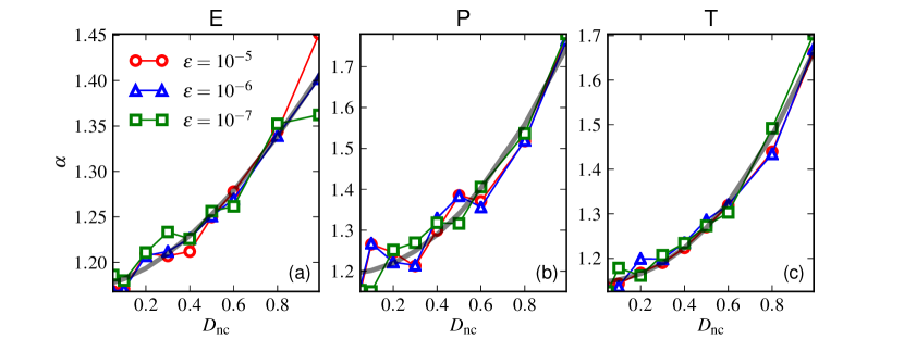
Figure 10.: Variations of power-law indices for the PDFs of (a) total avalanche energy, (b) peak energy release and (c) duration, as a function of the conservation parameter [$D_{\rm nc}$] and for various driving rates [$\varepsilon$], as labeled. The grey thick line corresponds to the power-law fit (see text). All these runs are for NC0-type models.fig:alphancons

Finally, the waiting-time distributions obtained in these nonconservative models show the same overall qualitative behavior as those characterizing the conservative models (see Figures fig:wtdcons and fig:Ewtd).

3.3 On the Breaking of Finite-Size Scalingssec:fss

In statistical physics parlance, the appearance of several statistically distinct populations of avalanches (as occurs here) represents a break of finite-size scaling. Such breaks are known to occur in certain classes of SOC models. For instance, the Olami, Feder, and Christensen (1992) model for earthquake, which is also a globally and deterministically driven model, shows a clear break in finite-size scaling when its nonconservation parameter (equivalent to $1-D$ herein) becomes too small (see Grassberger, 1994). This can be traced to the effect of boundaries on internal avalanche dynamics, with lattice nodes located near the boundaries becoming favored triggering sites for large avalanches (see Lise and Paczuski, 2001). We have searched for spatial dependencies in the triggering sites of large avalanches in a few simulation runs, by constructing 2D spatial frequency distributions functions for onset locus of large and small avalanches. No obvious dependencies on the distance to boundaries could be detected.

We explored the effect of resolution on the break of finite-size scaling at both ends of our PDF (Figure fig:resolution). We observe that the population of large and quasi periodic avalanches always spans the last decade of energies (both peak and total) for the four sizes of lattice we considered. It confirms that this population consists of avalanches spanning the whole lattice and does not result from a particular scale our model could have introduced.

The small avalanches population is on the contrary sensitive to the lattice resolution. The avalanche duration PDF (c) shows no hint of resolution effect: the small avalanches population results from a shift of the typical energy an avalanche of small duration is able to release. We reiterate that the plateau of small avalanches originates from the fact that small avalanches have the ability to release energies in a significantly larger range (spanning higher energies) than the corresponding avalanches of the LH model. Calculating the energy [$\Delta e_{NC0}$] released by a one-node and one-iteration avalanche in model NC0 (Equation (eq:erel1), we obtain:

$$\ilabel{eq:energy_{r}eleased_{N}C0}\frac{\Delta e_{NC0}}{e_{0}}=\frac{\Delta e_{i,j}}{e_{0}}+\frac{1-r_{0}}{2Z_{c}}\sum\left(A_{i\pm 1,j\pm 1}\right)+\frac{1-r_{0}^{2}}{5}\,,$$ (17)

where we recall that $r_{0}\in[D,1]$. If $r_{0}=1$, we obtain the classical LH energy release (Equation (eq:erel1). If $r_{0}\approx D$, the additional energy release is dominated by the second term – involving the sum of the nodal variable over the neighbouring node – which is of the order of the nodal variable. The worst case occurs in the middle of the lattice where the nodal variable is maximal. A larger lattice leads to larger values of the nodal variable, which explains the wider small avalanches populations observed in Figure fig:resolutiona – b. For example, the nodal variable is of the order of $3\times 10^{4}$ for a lattice of $384^{2}$, which corresponds indeed to the energy limit distinguishing the small avalanches from the scale-free mid-size ones. Finally, the range of power-law mid-size avalanches also increases with resolution, as expected from classical results of the LH model.

Unlike in the seismic-fault model (which should be thought of, in some global sense, as periodic), here coronal loops do have a finite spatial extent in cross-section, and so the various “tricks” that have been developed to restore finite-size scaling to the Olami et al. model (e.g. Manna and Bhattacharya, 2006) cannot legitimately be used in the present context.

The model results of Grassberger (1994) suggested that the loss of finite-size scaling takes place quite suddenly, beyond a certain level of non-conservation. The results reported here indicate a more gradual transition, with the population of large, quasiperiodic avalanches gradually merging with the mid-size, scale-free avalanches as $D$ decreases (Figure fig:pdfncons).

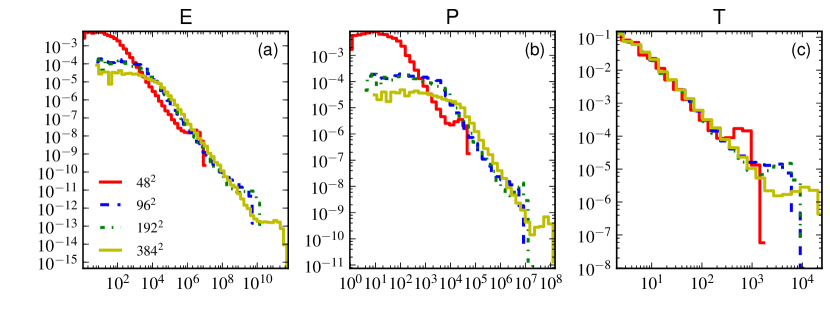
Figure 11.: PDFs of E, T, and P for model NC0 [$D_{nc}=0.8$, $\varepsilon=10^{-5}$] for four different lattice sizes.fig:resolution

4 Discussion and Conclusion sec:conclusion

In this article, we have described and documented the behavior of a novel and hitherto unexplored class of lattice-based avalanche models applicable to solar flares. These models, based on a spatially global and fully deterministic driving mechanism, are amenable to physical interpretation in terms of slow twisting of a small coronal loop. Stochasticity is introduced in the models at the level of the redistribution rules and stability threshold governing avalanching dynamics.

Over significant portions of model space, the simulations produce three distinct populations of avalanches. The first is composed of the smallest avalanches with a plateau-like distribution. Then, a classical scale-free distribution of avalanches takes place in the mid-size range of energies. Finally, quasi-periodic avalanches with a more-or-less well-defined mean size make up the third population. The two latter populations are observed to merge in the context of avalanche models incorporating non-conservative redistribution rules.

We have argued that the large, quasiperiodic avalanches are the reflection of an energy loading/unloading cycle driven by our adopted global deterministic driving mechanism. Even though an avalanche is always triggered at a single lattice node, the effect of the global driver is that energy has been accumulating at all internal lattice nodes prior to avalanche onset. Once the avalanche begins, this energy must be either evacuated at the open boundaries, or dissipated locally within the lattice (in non-conservative models). In conservative models, only the former is possible, which leads inevitably to the buildup of very large avalanches that must connect to the boundaries – and thus end up spanning the whole system – and remain active until the excess energy has been drained away from the lattice – thus producing long duration avalanches. In that respect, it is therefore not surprising that a distinct population of large avalanches (and, consequently, break of finite-size scaling) is most readily observed in models based on conservative redistribution rules.

We have been careful thus far to refrain from declaring our models to be in a true self-organized critical state, using instead the term “SOC-like” to characterize their avalanching behavior. Formal demonstration of SOC typically requires the computation of critical exponents, and the demonstration that the latter satisfy mutual numerical relations that place them in a specific universality class. Although interesting in and of itself, the identification of the universality class to which the present model belongs is of limited interest from the point of view of flare modelling. We stress again that the models discussed in this article do satisfy all sine qua non physical conditions believed to be required for SOC (Jensen, 1998): a slowly driven open system subjected to a self-limiting, local, finite-threshold instability. Moreover, in nonconservative models characterized by no quasi-periodic large scale events, the lack of dependence of the power-law indices of avalanches size and duration on the driving rate and lattice size certainly suggests that these models all belong to the same universality class.

Although non-conservative redistribution rules have received, to the best of our knowledge, little attention in the solar flare context, true SOC avalanching behavior is known to materialize in non-conservative system. The most studied such SOC system is the cellular automaton formulation of the stick–slip model for earthquake, introduced by Olami, Feder, and Christensen (1992). In that model, non-conservation is related to the fact that a moving block exerts a force not only on its neighbour blocks via the connecting springs, but also on the two plates bounding (and driving) the system from above and below; hence; when an individual block moves, a fraction of the potential energy stored in the springs is dissipated as heat via friction against the bounding plates, rather than all of it ending up in other springs by the end of the avalanche. Something similar also takes place in the non-conservative substorm models of Liu et al. (2006) and Vallières-Nollet et al. (2010). There, a fraction of the energy released by an unstable magnetic flux tube within the central (equatorial) plasma sheet is lost via MHD waves and/or charged particles travelling away along magnetic field lines back towards Earth, eventually leading to auroral excitation in polar regions. A particularly interesting feature of the latter model is its ability to simultaneously produce “internal” avalanches with a scale-free size distribution, and quasi-periodic boundary discharge avalanches with a well-defined mean-size. This squares well with the statistically distinct properties of auroral emission on the one hand, and ring current injection events on the other, both being in principle related manifestation of energy release events in the central plasma sheet. In the model of Liu et al. (2006), this effect materialized in part because the boundaries were set up so as to respond dynamically to incoming avalanches; the results presented herein indicate that dual populations of energy release events, each with distinct statistical characteristics, would still materialize in such globally driven systems, even with more conventional “open” boundary conditions, provided conservation is high enough. Finally, solar flares also exhibit non-conservative properties. Flares are thought to originate from reconnection processes in coronal loops that feed on the stored magnetic energy. Along with the magnetic reorganization associated with a flare, some energy is systematically lost from the system either through radiation (direct X-ray emissions, or hard X-ray emissions triggered by reconnection-accelerated energetic particles), accelerated particles escape or even conduction along the magnetic field lines. We modeled those effects with a simple non-conservation parameter in the avalanching process. Albeit with a quite different cellular automaton model, our results are consistent with the previous finding of Hamon, Nicodemi, and Jensen (2002): a quasi-cyclic population of large avalanches is found in both cases when the model is close to be purely conservative.

Notwithstanding the presence or absence of a population of small and large avalanches, in the realm of mid-size avalanches all models are characterized by a power-law distribution of avalanche energy release spanning many orders of magnitude. In general, the corresponding power-law indices are somewhat smaller than for the LH model, implying flatter PDFs, so that all models have a power-law index smaller than the critical value $\alpha_{E}=2$ above which the smaller flares (i.e. avalanches) would become the dominant contributors to coronal heating, as in Parker’s nanoflare hypothesis.

An obvious extension of the present model is to introduce the third spatial dimension; as argued in Section ssec:phys, the 2D lattices considered herein can be best regarded as a cross section at some fixed position along a coronal loop. Evidently, allowing avalanches to develop along the loop’s length would yield a more realistic model. In particular, it would become possible to map the 3D lattice to a bent coronal loop, and therefore compute fractal dimensions of flares/avalanches (see, e.g. Morales and Charbonneau, 2009) in the same manner as carried out from observations (see, e.g. Aschwanden, Zhang, and Liu, 2013). This would open a new comparative bridge between modelling and observation.

The broad exploration of parameter space made possible with the computationally much less demanding 2D lattices has allowed us to pinpoint the most important parameter regime, which is found for highly dissipative redistribution. Then, the way in which stochasticity is introduced in the model (stability threshold, extraction, redistribution rules) plays a comparatively lesser role in determining the size distribution of avalanches. In other words, the models are robust with respect to the details of stochastic effects.

The present model finally provides an interesting basis for a practical use of avalanches models in the context of solar flares (Strugarek and Charbonneau, 2014). The deterministic driver minimizes the level of stochasticity embedded in the model, which results in very good predictive capabilities for the larger events. Interestingly, our model could provide an efficient and cheap alternative method for the prediction of large solar flares in the context of space weather.

Acknowledgements

The authors acknowledge stimulating discussions during the ISSI Workshops on Turbulence and Self-Organized Criticality (2012 – 2013) held in Bern (Switzerland); and during the “Festival de théorie” (2013) held in Aix-en-Provence (France). We acknowledge support from Canada’s Natural Sciences and Engineering Research Council.

References

- Aschwanden (2011) Aschwanden, M.J.: 2011, The State of Self-organized Criticality of the Sun During the Last Three Solar Cycles. I. Observations. Sol. Phys. 274(1), 99. DOI. ADS.
- Aschwanden and Charbonneau (2002) Aschwanden, M.J., Charbonneau, P.: 2002, Effects of Temperature Bias on Nanoflare Statistics. ApJ 566(1), L59. DOI. ADS.
- Aschwanden and Parnell (2002) Aschwanden, M.J., Parnell, C.E.: 2002, Nanoflare Statistics from First Principles: Fractal Geometry and Temperature Synthesis. ApJ 572(2), 1048. DOI. ADS.
- Aschwanden, Zhang, and Liu (2013) Aschwanden, M.J., Zhang, J., Liu, K.: 2013, Multi-wavelength Observations of the Spatio-temporal Evolution of Solar Flares with AIA/SDO. I. Universal Scaling Laws of Space and Time Parameters. ApJ 775(1), 23. DOI. ADS.
- Aschwanden et al. (2000) Aschwanden, M.J., Tarbell, T.D., Nightingale, R.W., Schrijver, C.J., Title, A., Kankelborg, C.C., Martens, P., Warren, H.P.: 2000, Time Variability of the “Quiet” Sun Observed with TRACE. II. Physical Parameters, Temperature Evolution, and Energetics of Extreme-Ultraviolet Nanoflares. ApJ 535(2), 1047. DOI. ADS.
- Aschwanden et al. (2007) Aschwanden, M.J., Winebarger, A., Tsiklauri, D., Peter, H.: 2007, The Coronal Heating Paradox. ApJ 659(2), 1673. DOI. ADS.
- Bak, Tang, and Wiesenfeld (1987) Bak, P., Tang, C., Wiesenfeld, K.: 1987, Self-organized criticality - An explanation of 1/f noise. Phys. Rev. Lett. 59, 381. DOI. ADS.
- Bareford, Browning, and van der Linden (2010) Bareford, M.R., Browning, P.K., van der Linden, R.A.M.: 2010, A nanoflare distribution generated by repeated relaxations triggered by kink instability. A&A 521, 70. DOI. ADS.
- Baty and Heyvaerts (1996) Baty, H., Heyvaerts, J.: 1996, Electric current concentration and kink instability in line-tied coronal loops. A&A 308, 935. ADS.
- Charbonneau (2013) Charbonneau, P.: 2013, SOC and Solar Flares. In: Self-Organized Criticality Systems, Open Academic Press, 404. ADS
- Charbonneau et al. (2001) Charbonneau, P., McIntosh, S.W., Liu, H.-L., Bogdan, T.J.: 2001, Avalanche models for solar flares (Invited Review). Sol. Phys. 203(2), 321. DOI. ADS.
- De Pontieu et al. (2011) De Pontieu, B., McIntosh, S.W., Carlsson, M., Hansteen, V.H., Tarbell, T.D., Boerner, P., Martinez-Sykora, J., Schrijver, C.J., Title, A.M.: 2011, The Origins of Hot Plasma in the Solar Corona. Science 331(6), 55. DOI. ADS.
- Dennis (1985) Dennis, B.R.: 1985, Solar hard X-ray bursts. Sol. Phys. 100, 465. DOI. ADS.
- Grassberger (1994) Grassberger, P.: 1994, Efficient large-scale simulations of a uniformly driven system. Phys. Rev. E 49(3), 2436. DOI. ADS.
- Hamon, Nicodemi, and Jensen (2002) Hamon, D., Nicodemi, M., Jensen, H.J.: 2002, Continuously driven OFC: A simple model of solar flare statistics. A&A 387, 326. DOI. ADS.
- Jensen (1998) Jensen, H.J.: 1998, Self-Organized Criticality: Emergent Complex Behavior in Physical and Biological Systems, Cambridge University Press,
- Kadanoff et al. (1989) Kadanoff, L.P., Nagel, S.R., Wu, L., Zhou, S.-M.: 1989, Scaling and universality in avalanches. Phys. Rev. A 39(1), 6524. DOI. ADS.
- Klimchuk (2006) Klimchuk, J.A.: 2006, On Solving the Coronal Heating Problem. Sol. Phys. 234(1), 41. DOI. ADS.
- Lise and Paczuski (2001) Lise, S., Paczuski, M.: 2001, Scaling in a nonconservative earthquake model of self-organized criticality. Phys. Rev. E 64(4), 46111. DOI. ADS.
- Liu et al. (2006) Liu, W.W., Charbonneau, P., Thibault, K., Morales, L.: 2006, Energy avalanches in the central plasma sheet. Geophys. Res. Lett. 33(1), 19106. DOI. ADS.
- Liu et al. (2011) Liu, W.W., Morales, L.F., Uritsky, V.M., Charbonneau, P.: 2011, Formation and disruption of current filaments in a flow-driven turbulent magnetosphere. J. Geophys. Res. 116(A), 3213. DOI. ADS.
- Lu (1995) Lu, E.T.: 1995, The Statistical Physics of Solar Active Regions and the Fundamental Nature of Solar Flares. ApJ 446, L109. DOI. ADS.
- Lu and Hamilton (1991) Lu, E.T., Hamilton, R.J.: 1991, Avalanches and the distribution of solar flares. ApJ 380, L89. DOI. ADS.
- Lu et al. (1993) Lu, E.T., Hamilton, R.J., McTiernan, J.M., Bromund, K.R.: 1993, Solar flares and avalanches in driven dissipative systems. ApJ 412, 841. DOI. ADS.
- Manna and Bhattacharya (2006) Manna, S.S., Bhattacharya, K.: 2006, Self-organized critical earthquake model with moving boundary. European Phys. J. 54(4), 493. DOI. ADS.
- McIntosh (2000) McIntosh, S.W.: 2000, On the Inference of Differential Emission Measures Using Diagnostic Line Ratios. ApJ 533(2), 1043. DOI. ADS.
- McIntosh and Charbonneau (2001) McIntosh, S.W., Charbonneau, P.: 2001, Geometric Effects in Avalanche Models of Solar Flares: Implications for Coronal Heating. ApJ 563(2), L165. DOI. ADS.
- Morales and Charbonneau (2009) Morales, L., Charbonneau, P.: 2009, Geometrical Properties of Avalanches in a Pseudo-3D Coronal Loop. ApJ 698(2), 1893. DOI. ADS.
- Norman et al. (2001) Norman, J.P., Charbonneau, P., McIntosh, S.W., Liu, H.-L.: 2001, Waiting-Time Distributions in Lattice Models of Solar Flares. ApJ 557(2), 891. DOI. ADS.
- Olami, Feder, and Christensen (1992) Olami, Z., Feder, H.J.S., Christensen, K.: 1992, Self-organized criticality in a continuous, nonconservative cellular automaton modeling earthquakes. Phys. Rev. Lett. 68(8), 1244. DOI. ADS.
- Parker (1983a) Parker, E.N.: 1983a, Magnetic Neutral Sheets in Evolving Fields - Part Two - Formation of the Solar Corona. ApJ 264, 642. DOI. ADS.
- Parker (1983b) Parker, E.N.: 1983b, Magnetic neutral sheets in evolving fields. I - General theory. ApJ 264, 635. DOI. ADS.
- Parker (1988) Parker, E.N.: 1988, Nanoflares and the solar X-ray corona. ApJ 330, 474. DOI. ADS.
- Priest, Heyvaerts, and Title (2002) Priest, E.R., Heyvaerts, J.F., Title, A.M.: 2002, A Flux-Tube Tectonics Model for Solar Coronal Heating Driven by the Magnetic Carpet. ApJ 576(1), 533. DOI. ADS.
- Robinson (1994) Robinson, P.A.: 1994, Self-organized criticality involving vector fields and random driving. Phys. Rev. E 49(3), 1984. DOI. ADS.
- Rosner and Vaiana (1978) Rosner, R., Vaiana, G.S.: 1978, Cosmic flare transients - Constraints upon models for energy storage and release derived from the event frequency distribution. ApJ 222, 1104. DOI. ADS.
- Strugarek and Charbonneau (2014) Strugarek, A., Charbonneau, P.: 2014, Predictive capabilites of avalanche models for solar flares. Submitted to Solar Physics.
- Vallières-Nollet et al. (2010) Vallières-Nollet, M.A., Charbonneau, P., Uritsky, V., Donovan, E., Liu, W.: 2010, Dual scaling for self-organized critical models of the magnetosphere. J. Geophys. Res. 115(A), 12217. DOI. ADS.
- Wheatland (2000) Wheatland, M.S.: 2000, The Origin of the Solar Flare Waiting-Time Distribution. ApJ 536(2), L109. DOI. ADS.
- Wheatland and Glukhov (1998) Wheatland, M.S., Glukhov, S.: 1998, Flare Frequency Distributions Based on a Master Equation. ApJ 494, 858. DOI. ADS.