See pages 1-18 of Manuscript_ArXiv2_noPageNumbers.pdf See pages 1 of Fig1.pdf See pages 1 of Fig2.pdf See pages 1 of Fig3.pdf See pages 1 of Fig4.pdf See pages 1 of Fig5.pdf

Table S1: Model parameters. Parameters above the horizontal line are used in the same way as in Ref. (11).

Name	Symbol	Value
Slider length ($x$)	$L$	$140\text{\,}\mathrm{mm}$
Slider height ($z$)	$H$	$75\text{\,}\mathrm{mm}$
Slider width ($y$)	$B$	$6\text{\,}\mathrm{mm}$
Number of blocks	$N_{x}$	$57$
	$N_{z}$	$31$
Slider mass	$M$	$75.6\text{\,}\mathrm{g}$
Block mass	$m$	$M/(N_{x}N_{z})$
Young’s modulus	$E$	$3\text{\,}\mathrm{GPa}$
Bulk spring modulus	$k$	$3BE/4$
Bulk spring length	$l$	$L/(N_{x}-1)=H/(N_{z}-1)$
Damping coefficient	$\eta$	$\sqrt{0.1km}$
Normal load	$F_{N}$	$1920\text{\,}\mathrm{N}$
Elastic foundation modulus	$k_{f}$	$k/2$
Driving spring modulus	$K$	$4\text{\,}\mathrm{MN}\text{\,}{\mathrm{m}}^{-1}$
Driving height	$h$	$5\text{\,}\mathrm{mm}$
Driving speed	$V$	$0.4\text{\,}\mathrm{mm}\text{\,}{\mathrm{s}}^{-1}$
Threshold force coefficient	$\mu_{s}=f_{\mathrm{thres}}/f_{N}$	$0.4$
Slipping force coefficient	$\mu_{d}=f_{\mathrm{slip}}/f_{N}$	$0.17$
Number of interface springs per block	$N_{s}$	$100$
Interface spring stiffness	$k_{ij}$	$\sqrt{$39.2\text{\,}\mathrm{G}\mathrm{N}\mathrm{/}\mathrm{m}^{2}$f_{N,ij}}$
Slipping time mean	$\mathrm{bar}t_{R}$	$2\text{\,}\mathrm{ms}$
Slipping time standard deviation	$\delta t_{R}$	$0.6\text{\,}\mathrm{ms}$
Triggering region width	$x_{\mathrm{trigger}}$	$22.5\text{\,}\mathrm{mm}$
Triggering region prestress	$\mathrm{bar}\tau_{\mathrm{trigger}}$	0.3
Time step duration	$\Delta t$	$2\cdot 10^{-7}\text{\,}\mathrm{s}$
Extra damping coefficient	$\alpha$	$\eta/40$

Supporting Methods

This section supplements the model description found in the main text and its Methods section with detailed information on how we initialize the system and apply the boundary conditions. We also provide some additional information on the simplified model.

The slider is initialized with full normal load $F_{N}$ and no tangential load $F_{T}$ by gradually applying $F_{N}$ without allowing springs to break, a technicality required because the normal forces on the springs, $f_{Nij}$, start at zero and therefore springs, if allowed to, would break under any stretching. We distribute the load $F_{N}$ uniformly on the top blocks; apart from this we use the same non-frictional boundary conditions as in (11). The unique equilibrium is found through damped relaxation of typical duration $10\text{\,}\mathrm{ms}$. After relaxation, we check that no spring is stretched beyond its strength and introduce the driving spring starting from zero applied driving force $F_{T}$. Then $F_{T}$, which acts on the block on the left side of the slider situated at height $h$ above the interface, through the driving spring, increases as the driving point moves to the right with speed $V$.

In the simplified model used for Fig. 3D, we disregard the microscopic state by using a single friction spring per block. Taking parameters from the microscopic reference model described in the main text, each block’s spring now has a strength $\tau_{\text{thres}}=\mu_{s}p_{i}=N_{s}f_{\text{thres}}$. The stiffness $k_{i}$ of a block’s friction spring equals the combined stiffness of the springs per block in the reference model. The force on block $i$ from its friction spring is $f_{Ti}=k_{i}(x_{is}-x_{i})$, where $x_{is}$ is the attachment point of the spring to the track. Upon breaking, the spring becomes a slipping spring and its behaviour starts to differ from that of the springs in the microscopic model. We impose a slow slip by letting $x_{is}$ move with a velocity $v_{\text{slow slip spring}}$ for a time $t_{\text{slow slip spring}}=\mathrm{bar}t_{R}$. This process competes with the dynamic friction law where the spring trails the block with $x_{is}$ adjusted in every time step to ensure $\lvert f_{Ti}\rvert\leq\mu_{d}p_{i}$, so that the spring attachment point moves with the highest of $v_{\text{slow slip spring}}$ and $v_{xi}$, the speed of the block in the $x$-direction. When the block motion reverses ($v_{xi}$ changes sign) the spring returns to the pinned state, but $x_{is}$ continues to move at $v_{\text{slow slip spring}}$ until $t_{\text{slow slip spring}}$ after the spring broke.

The systematic studies leading to Fig. 3C (inset, green), 3D and 4D were done with different normal forces and different initialization from the other simulations. The normal force boundary conditions on the top and bottom were exchanged: this simplifies the analysis by setting a constant normal force $p_{i}=F_{N}/N_{x}$ on all blocks $i$ at the interface. To maintain stability against global rotation, the top blocks interacted with an elastic ceiling with the same properties as the elastic foundation used in Ref. (11) and the other simulations presented here.

To obtain an initial state with a prescribed interfacial shear stress profile we turned the interface springs off during the initialisation. In their place we added to each bottom block the force corresponding to the shear stress to be prescribed. We also introduced the driving spring, but let $V=0$. During relaxation, the sample moved along the $x$-axis until the force in the driving spring balanced the net force from the interfacial shear stress. To get rid of oscillations more efficiently we added damping forces $-\alpha(\vec{v}_{i})$ on the blocks’ motion. After relaxation, the extra forces and the extra damping were turned off and the interfacial springs were introduced, with their attachment points $x_{ij}$ chosen such that the net force on each block was unchanged and the desired distribution of spring forces, $\phi(f_{T})$, appeared. We then waited a few timesteps to ensure that the transition from pre- to post-relaxation involved no force discontinuities. Next, instead of driving the system with $V\neq\-0$ until rupture was triggered, we started fronts by depinning simultaneously all springs for all blocks to the left of $x_{\text{trigger}}$. The shear stress in the triggering region has a strong influence on the rupture fronts; in order to compare results between simulations we used a constant value $\mathrm{bar}\tau_{\text{trigger}}$.

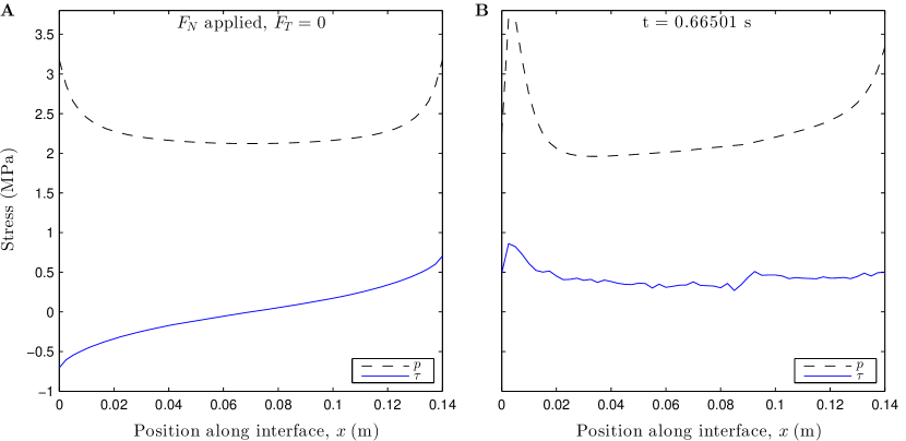
Figure S1: Spatial distributions of normal ($p$) and shear ($\tau$) stresses from the simulation behind events I–III. (A) The initial state with full normal load $F_{N}$ and no tangential load $F_{T}$ (see Supporting Methods). The normal stress $p(x)$ is symmetric, with edge effects related to the flat punch geometry of the contact. The shear stress $\tau(x)$ is antisymmetric, due to Poisson expansion being restricted at the interface by friction. (B) The state just before event I. The application of $F_{T}$ has modified both the shear stress profile and the normal stress profile (due to the friction-induced torque arising when $F_{T}$ is applied at a finite height $h$ above the interface).

Figure S2: A fast-slow event arising spontaneously in a simulation using the simplified friction law with a single interface spring per block. The parameter $v_{\mathrm{slow}\,\mathrm{slip}\,\mathrm{spring}}=$1.5\text{\,}\mathrm{mm}\text{\,}{\mathrm{s}}^{-1}$$ (Supporting Methods). (A) Spatio-temporal plot of the instantaneous friction to normal force ratio. (B) Rupture front speed $v_{c}$. Block rupture is defined to occur when the interface spring depins. Front speed is measured as in Fig. 2.

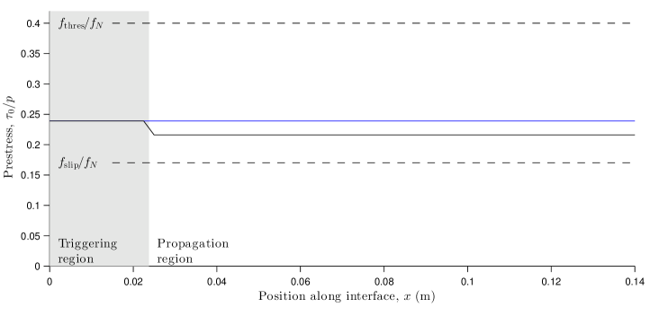
Figure S3: Spatial distributions of prestress $\tau_{0}/p$ for prepared states of the interface. In the front triggering region on the left, the prestress is $\mathrm{bar}\tau_{0}=\left(\frac{\tau_{0}}{p}-\frac{f_{\mathrm{slip}}}{f_{N}}\right)/\left(\frac{f_{\mathrm{thres}}}{f_{N}}-\frac{f_{\mathrm{slip}}}{f_{N}}\right)=0.3$ for all prepared states used in Fig. 3D, 4C and 4D. In the front propagation region the prestress is homogeneous along the interface, at a value varied between prepared states, here $\mathrm{bar}\tau_{0}=0.2$ (black) and $\mathrm{bar}\tau_{0}=0.3$ (blue). After initialization, all springs in the triggering region are depinned simultaneously. Initiating the events in this way, rather than by driving the system until rupture is triggered, ensures that the force drop / energy release in the triggering region remains the same between simulations.

The non-dimensional form $\mathrm{bar}\tau_{0}$ of the prestress represents the ratio between (i) the stress in excess of the stress obtained during sliding and (ii) the maximum dynamic stress drop that results from rupture. It is analogous to the so-called $S$ classically used in seismology and to the form defined in Ref. (11).

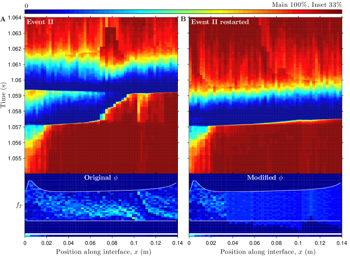
Figure S4: Microscopic force distributions significantly affect rupture fronts. The data in Fig. 4A,B repeated with spring force distributions shown in detail. (A) Event II shown as in Fig. 2. (B) Simulation behind A restarted at $1.054\text{\,}\mathrm{s}$ with a wider distribution $\phi(f_{T})$ of shear forces results in a fast-only event. Insets: For each block along the interface, a color coded histogram of $\phi(f_{T})$ at $1.054\text{\,}\mathrm{s}$. The vertical axis shows the force level in individual springs, which extends up to $f_{\mathrm{thres}}$. The level $f_{\mathrm{thres}}$ is shown by the upper white line; it is different for each block because it varies with normal force. The lower white line corresponds to $f_{T}=$0\text{\,}\mathrm{N}$$. The color denotes the fraction of springs found at each value of $f_{T}$ using an arbitrary bin width. This means that (apart from normalization) each vertical slice in the insets shows the same type of data as Figure S5A. Offset data: Fraction of slipping springs at $1.054\text{\,}\mathrm{s}$.

In order to isolate the effect of $\phi(f_{T})$ on front propagation from the influence of front initiation and stress state we leave the loading zone on the left unmodified (it is the same in both insets) so that the restarted event begins like the original; we also let the modified $\phi(f_{T})$ have the same mean value as the original $\phi(f_{T})$ for all blocks. Thus, the stress state is the same and the only change is in the width of $\phi$.

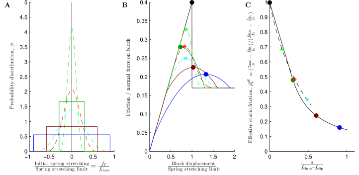
Figure S5: Dependence of effective static friction coefficient $\mu_{s}^{\mathrm{eff}}=\tau_{\mathrm{max}}/p$ on the distribution $\phi$ of forces in the interface springs. (A) Uniform and bell-shaped initial distributions of various widths. The bell-shaped distributions are polynomials with roots at $\pm a$ and the functional form $\phi(\xi)=5/(4a)(1+3\lvert\xi/a\rvert)(1-\lvert\xi/a\rvert)^{3},\xi\in[-a,a]$. (B) Friction to normal force ratio vs block displacement for a block having the spring force distributions in A (corresponding colours). Spring relaxation during slip is excluded from the calculation, a valid assumption when the passage of the rupture front is quick compared to the mean slipping time $\langle t_{R}\rangle$. Markers are located at maxima, which define $\tau_{\mathrm{max}}/p$. (C) Effective static friction coefficient vs $\sigma$, the standard deviation of $\phi$. Each marker takes its abscissa from the data in A and its ordinate from B. Drawn and dashed lines connect markers corresponding to uniform and bell-shaped $\phi$, respectively. They are used in Fig. 4C as reference lines for simulation data. For clarity, only a few of the $\phi$ that were used to determine the lines are shown on this figure.

The form $\mathrm{bar}\mu_{s}^{\mathrm{eff}}$ is analogous to $\mathrm{bar}\tau_{0}$ introduced in Figure S3, and represents the ratio of (i) the dynamic stress drop from the effective static friction level to the stress obtained during sliding and (ii) the maximum value this stress drop can attain.

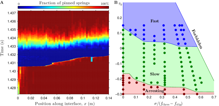
Figure S6: Results from an alternative model with a different individual behaviour of the interface springs, showing the robustness of our results against changes in the interfacial law. (A) A spontaneously arising fast-slow-fast event, analogous to that in Fig. 2A. (B) Observed front type for prepared interfaces, analogous to Fig. 4D.

All data in this figure comes from simulations with a model in which the slipping force $f_{\mathrm{slip}}$ decreases linearly with time. This microscopic friction law modifies the slow slip mechanism with respect to the reference microscopic model. Until depinning, the springs have the same behaviour in both models. Upon entering the slipping state, the force from each spring on the block immediately drops to the level $f_{\mathrm{slip}}^{0}=\mu_{d}f_{N,ij}$, as in the reference model. Then the slipping force decays linearly in time with a decay rate depending on the slipping time and the force level at repinning $f_{\mathrm{new}}$; that is, $f_{\mathrm{slip}}=f_{\mathrm{slip}}^{0}-(f_{\mathrm{slip}}^{0}-f_{\mathrm{new}})t_{s}/t_{R}$, with $t_{s}$ measured from the time the spring entered the slipping state. The slipping time distribution is the same as in the reference model. The decay in the friction coefficient enables a slow slip motion after the initial rapid slip, which allows this model to sustain slow fronts for a relatively wide range of initial spring stretching configurations and stress states, as seen in B.

The parameters used with this model are the same as in the reference model (Table S1), except for $k_{ij}=\sqrt{$54.1\text{\,}\mathrm{G}\mathrm{N}\mathrm{/}\mathrm{m}^{2}$f_{N,ij}}$, $\mu_{d}=0.28$ and the new parameter $\mu_{\mathrm{new}}=0.7\mu_{d}\approx 0.2$ used to determine $f_{\mathrm{new}}=\mu_{\mathrm{new}}f_{N,ij}$.

Supporting Equations

Estimate of $v_{\mathrm{slow}\,\mathrm{slip}}$ from model parameters

Here we provide the arguments behind the slow slip speed estimate used in the inset of Fig. 3C.

The mechanism for slow slip in our model is the force drop when slipping junctions relax and repin at zero force. To determine the slip speed (block motion per unit time) associated with the relaxation of junctions, we identify the net slip caused by this change and the time over which the change happens. To do this, we assume that each time a junction relaxes, the block moves forward just enough to return to the force it was bearing just before relaxation. Thus, the force reduction $-f_{\text{slip}}$ in the junction is matched by an equivalent net force increase in the junctions that are already pinned and in the coupling to the neighbouring blocks. The effective stiffness of these interface and bulk terms depend on the fraction of junctions that are pinned and on the motion of the neighbouring blocks, respectively.

A careful look at the motion of blocks during their slow slipping regime proved that neighbouring blocks move essentially at the same slow slip speed. This means that the force changes on a block due to relative motion with respect to its neighbours remain negligible. We can therefore assume in this calculation that the only contribution to force restoring after junction relaxations is due to the pinned interfacial junctions.

We now assume that all junctions start in the slipping state. After the first junction relaxes and repins, the effective stiffness of the interface is just the stiffness of this single junction, $k_{ij}$. The force drop $-f_{\text{slip}}$ must be compensated by stretching this (now pinned) junction by moving the block a distance $\delta_{1}=f_{\text{slip}}/k_{ij}$. For the second junction the force drop is again $-f_{\text{slip}}$, but the stiffness of the interface has increased to $2k_{ij}$ and the required slip is $\delta_{2}=f_{\text{slip}}/(2k_{ij})$. If no junction would reach its breaking threshold $f_{\text{thres}}$ during the whole relaxation process, then we would find $x_{\text{slow slip}}=\sum_{j=1}^{N_{s}}\delta_{j}=\sum_{j=1}^{N_{s}}f_{\text{slip}}/(jk_{ij})$. Since the $k_{ij}$ are independent of $j$ this is just $\delta=f_{\text{slip}}/k_{ij}\sum_{n=1}^{N_{s}}1/n$ with $n$ a dummy index. For $N_{s}=100$ used in the model, the sum evaluates to $5.2$. However, for $f_{\text{thres}}/f_{\text{slip}}=40/17$ used in the model, some junctions do break again before all slipping junctions relax. The force drop associated with the transition from pinned to slipping state is $f_{\text{slip}}-f_{\text{thres}}$, and acts in the same way as the force drop when junctions leave the slipping state. Taking this into account and evaluating the return to the pinned state more carefully, we find the net block slip to be $8.5f_{\text{slip}}/k_{ij}$.

With the slipping time standard deviation $\delta t_{R}=0.3\mathrm{bar}t_{R}$ used in the model, the time for all the junctions to return to the pinned state is found to be close to $2\langle t_{R}\rangle$.

Combining these slip distance and slip time values, and defining $\tau_{\text{slip}}=N_{s}f_{\text{slip}}$ and $k_{i}=N_{s}k_{ij}$, we use

$$v_{\text{slow slip, estimate}}=4.2\frac{\tau_{\text{slip}}}{k_{i}\langle t_{R}\rangle}.$$ (1)

The inset of Fig. 3C plots the slow slip speed measured in the simulations against this estimate. The markers indicate when we have varied $\tau_{\text{slip}}$ ($\blacksquare$), $k_{i}$ ($\blacktriangleleft$) and $\langle t_{R}\rangle$ ($\blacktriangle$). $\bullet$ uses our reference parameters. The blue data is based on restarting event II. Because $\tau_{\text{slip}}$ and $k_{i}$ enter in the elastic state of the slider, only $\langle t_{R}\rangle$ could be varied for these simulations. The green data is for prepared homogeneous interfaces, where parameters can be varied freely.

When slow slip speed is measured in the simulations based on event II (blue data in inset of Fig. 3C), some deviation from $v_{\text{slow slip, estimate}}$ are observed. There are several possible reasons for such a deviation. First, the assumption of co-moving neighbours is only approximately correct (near the front tip the neighbours to the right are stuck until the rupture front passes them). The actual motion of the neighbours also depends on the stress state and the triggering of the event. Second, the assumption of force re-balancing every time a junction changes state is probably too strong.

Scaling of $v_{c,\mathrm{slow}}$ with $v_{\mathrm{slow}\,\mathrm{slip}}$

The data collapse in Fig. 3D is obtained by plotting the slow rupture speed $v_{c,\mathrm{slow}}$ against the quantity $v_{\mathrm{slow}\,\mathrm{slip}}k_{i}l_{0}/(\tau_{\mathrm{thres}}-\tau^{0})$, where $v_{\mathrm{slow}\,\mathrm{slip}}$ is the slow slip speed, $k_{i}$ is the stiffness of the connection between a block and the interface (a single spring in the simplified model and a parallel connection in the reference microscopic model), $l_{0}$ is a characteristic length, $\tau_{\mathrm{thres}}=N_{s}f_{\mathrm{thres}}$ is the maximum shear strength of a block and $\tau^{0}$ is the shear force in the propagation region before the event is started. In this section we provide a crude argument for this scaling.

When a region of initially homogeneous prestress is being stressed further by block motion on the left, the decaying shear force profile can be written on the form

$$\tau(x)=Af\left(\frac{x-x_{0}}{l_{0}}\right)+\tau^{0},$$ (2)

where $A$ is an amplitude and $f()$ is a function that has magnitude $1$ at $x=x_{0}$ and decays over a characteristic length $l_{0}$ that depends on the bulk to interfacial stiffness ratio $k/k_{i}$. The function $f()$ is known in 1D (Ref. (28), equation (46)); in 2D it can be measured in an elastostatic model, but its exact form is not required for the present argument.

In a static situation $\tau(x)$ is balanced by the friction forces in the interfacial springs. Ignoring the width of the spring force distribution, the block at $x_{0}$ is at its static friction threshold when the force on it from its neighboring blocks is $\tau(x_{0})=\tau_{\mathrm{thres}}$, which gives $A=(\tau_{\mathrm{thres}}-\tau^{0})$. The next block to the right, at position $x=x_{0}+\mathrm{d}x$, then has

$$\tau(x_{0}+\mathrm{d}x)=Af[x_{0}+\mathrm{d}x]+\tau^{0}.$$ (3)

Here we have used the short-hand notation $f[x]=f\big{(}(x-x_{0})/l_{0}\big{)}$.

As the front tip moves from the block at $x_{0}$ to the block at $x_{0}+\mathrm{d}x$, the force on this block from its neighbours increases to $\tau^{\prime}(x_{0}+\mathrm{d}x)=\tau_{\mathrm{thres}}$. It will be useful to rewrite this as $\tau^{\prime}(x_{0}+\mathrm{d}x)=\tau_{\mathrm{thres}}=\tau(x_{0})=Af[x_{0}]+\tau^{0}$. The change in force on the block at $x_{0}+\mathrm{d}x$ is

$$\Delta\tau(x_{0}+\mathrm{d}x) =\tau^{\prime}(x_{0}+\mathrm{d}x)-\tau(x_{0}+\mathrm{d}x)$$ (4)

$$=A(f[x_{0}]-f[x_{0}+\mathrm{d}x]).$$ (5)

Assuming a corresponding change in the friction force allows us to relate the force change to a displacement of the block, namely

$$\Delta u(x_{0}+\mathrm{d}x)=\frac{\Delta\tau(x_{0}+\mathrm{d}x)}{k_{i}}.$$ (6)

In the next step we will need the displacement of the block at $x_{0}$ during the same time interval. As the blocks are at closely spaced points in a deforming elastic medium we will assume $\Delta u(x_{0})=\Delta u(x_{0}+\mathrm{d}x)(1+O(\mathrm{d}x))\approx\Delta u(x_{0}+\mathrm{d}x)$.

Now we make the approximation that after breaking, the blocks move at a constant speed $v_{\mathrm{slow}\,\mathrm{slip}}$. It follows that the time it takes from when the block at $x_{0}$ breaks and until when the block at $x_{0}+\mathrm{d}x$ breaks is

$$\mathrm{d}t=\frac{\Delta u(x_{0})}{v_{\mathrm{slow}\,\mathrm{slip}}}.$$ (7)

During this time the front tip has moved the distance $\mathrm{d}x$ from one block to the next, and the front speed is

$$v_{c,\mathrm{slow}}=\frac{\mathrm{d}x}{\mathrm{d}t} =v_{\mathrm{slow}\,\mathrm{slip}}\frac{\mathrm{d}x}{\Delta u(x_{0})}$$ (8)

$$=v_{\mathrm{slow}\,\mathrm{slip}}\frac{k_{i}}{\tau_{\mathrm{thres}}-\tau^{0}}\frac{dx}{f[x_{0}]-f[x_{0}+\mathrm{d}x]}.$$ (9)

Here we recognize an approximation to the spatial derivative of the unknown function $f()$, evaluated at $x=x_{0}$. We will use the chain rule to separate the non-dimensional and dimensional parts of this derivative, and therefore we define $X(x)=(x-x_{0})/l_{0}$ so that $f[x]=f(X(x))$. With this notation,

$$\frac{\mathrm{d}f}{\mathrm{d}x} =\frac{\mathrm{d}f}{\mathrm{d}X}\frac{\mathrm{d}X}{\mathrm{d}x}=\frac{\mathrm{d}f}{\mathrm{d}X}\frac{1}{l_{0}}.$$ (10)

We arrive at

$$v_{c,\mathrm{slow}}=v_{\mathrm{slow}\,\mathrm{slip}}\frac{k_{i}}{\tau_{\mathrm{thres}}-\tau^{0}}\frac{l_{0}}{\left(-\frac{\mathrm{d}f}{\mathrm{d}X}\right)_{x=x_{0}}}.$$ (11)

This argument provides a rationale for the linear relationship observed in Fig. 3D, but with the function $f()$ unknown we are not able to predict the value of the coefficient of proportionality. From the shear force profiles we estimate the decay length $l_{0}=$7\text{\,}\mathrm{mm}$$, a value shared between simulations because we keep $k/k_{i}$ the same, and rescale $v_{\mathrm{slow}\,\mathrm{slip}}$ with $k_{i}l_{0}/(\tau_{\mathrm{thres}}-\tau^{0})$. Note that in the model, $\tau_{\mathrm{thres}}=N_{s}f_{\mathrm{thres}}=\mu_{s}p$, with $\mu_{s}$ the threshold force coefficient and $p$ the normal force on the block, which means that the normal force enters in the scaling.