Tails of weakly dependent random vectors

Abstract

We introduce a new functional measure of tail dependence for weakly dependent (asymptotically independent) random vectors, termed weak tail dependence function. The new measure is defined at the level of copulas and we compute it for several copula families such as the Gaussian copula, copulas of a class of Gaussian mixture models, certain Archimedean copulas and extreme value copulas. The new measure allows to quantify the tail behavior of certain functionals of weakly dependent random vectors at the log scale.

Key words: tail dependence, asymptotic independence, copulas, regular variation, Gaussian mixtures

MSC 2010: 60F10, 62G32

1 Introduction

The goal of this paper is to propose a new approach to describe asymptotic independence (weak tail dependence), and to use this approach to study the asymptotic behavior of tail probabilities like

$$\Pr[\min(X_{1},\dots,X_{n})\geq t]\quad\text{as $t\to\infty$}$$ (1)

or

$$\Pr[X_{1}+\dots+X_{n}\leq t]\quad\text{as $t\to 0$ with $X_{1}\geq 0,\dots,X_{n}\geq 0$.}$$ (2)

when the components of the vector $(X_{1},\dots,X_{n})$ are asymptotically independent.

In multivariate extreme value theory, asymptotic independence refers to the situation when the probability that any two components of a random vector are simultaneously large, on a suitable scale, is negligible compared to the probability that any one component is large. This ensures that suitably renormalized componentwise maxima of a sequence of independent copies of the vector become asymptotically independent. The components of an asymptotically independent random vector may be dependent in the usual sense. For instance, the multivariate Gaussian distribution is known to be asymptotically independent for any nondegenerate covariance matrix (Sibuya, 1959).

Asymptotic independence is a natural property which is often observed in the data coming from many different application domains (De Haan and De Ronde, 1998; Maulik et al., 2002; Draisma et al., 2004; Ledford and Tawn, 1997, 1996; Heffernan et al., 2005), and is an inherent feature of many widely used models, for example, in finance. In addition to the already mentioned multivariate Gaussian, one can quote, e.g., the multivariate generalized hyperbolic (Schlueter and Fischer, 2012), and more generally all Gaussian mixture models with exponentially decaying mixing variable (see Section 3 below). It is therefore important to understand the implications of asymptotic independence assumption on the tail behavior of random vectors.

In the literature, asymptotic independence is often introduced using the property of hidden regular variation (Resnick, 2002; Maulik and Resnick, 2004; Resnick, 2007), which is a refinement of the coefficient of tail dependence introduced in Ledford and Tawn (1996, 1997). Recall that a random vector $\boldsymbol{X}$ with values in $[0,\infty)^{n}$ is said to be multivariate regularly varying if there exists a function $b(t)\to\infty$ as $t\to\infty$ and a non-negative Radon measure $\nu\neq 0$ such that

$$t\Pr\Big{[}\frac{\boldsymbol{X}}{b(t)}\in\cdot\Big{]}\to\nu$$ (3)

as $t\to\infty$ in the sense of vague convergence of measures on the cone $E=[0,\infty]^{n}\setminus\{0\}$. Now, $\boldsymbol{X}$ is said to possess the property of hidden regular variation if in addition to (3), there exists a non-decreasing function $b^{*}(t)\to\infty$ such that $b(t)/b^{*}(t)\to\infty$ as $t\to\infty$ and a Radon measure $\nu^{*}\neq 0$ such that

$$t\Pr\Big{[}\frac{\boldsymbol{X}}{b^{*}(t)}\in\cdot\Big{]}\to\nu^{*}$$ (4)

on the cone $E^{*}:=E\setminus\cup_{i=1}^{n}L_{i}$, where $L_{i}$ is the i-th coordinate axis. In other words, under hidden regular variation, the probability $\Pr[X_{i}\geq x_{i}t,X_{j}\geq x_{j}t]$ for any $i\neq j$ decays regularly, but at a faster rate than the tail probabilities of individual components.

The theory of hidden regular variation along with its more recent extensions (Das et al., 2013) allows to quantify the asymptotic behavior of the tail probabilities like (1) or (2) but it is well suited for distributions with fat power-law tails and tail equivalent margins and does not readily apply to, say, models with exponential tail decay which are widely used in finance. An alternative (but related) approach to studying dependence within asymptotic independence, consists in observing that for, say, identically distributed positive random variables, asymptotic independence in the lower tail implies that

$$\lim_{x\downarrow 0}\frac{\Pr[X_{1}\leq x,\dots,X_{n}\leq x]}{\Pr[X_{1}\leq x]}=0,$$

and information about “residual” dependence may be extracted from the multivariate distribution function by studying a related limit on the logarithmic scale. This leads to the so called coefficient of weak tail dependence (Coles et al., 1999; Schlueter and Fischer, 2012; Hashorva, 2010; Heffernan, 2000) usually defined (for the case of the lower index of a two-dimensional copula $C$) as

$$\lim_{u\to 0}\frac{2\ln u}{\ln C(u,u)}-1.$$ (5)

This coefficient is defined at the level of copulas, and hence does not require strong assumptions on the margins. It exists under much less stringent conditions than those required for hidden regular variation (since here one is only interested in log-scale asymptotics), but the knowledge of the weak tail dependence coefficient does not provide information on the functionals like (1) or (2), which also depend on the margins.

In this paper, we develop a functional extension of the weak tail dependence coefficient (5), which we term weak tail dependence function. For the lower tail of the copula, the weak tail dependence function is defined by

$$\chi(\lambda_{1},\dots,\lambda_{n})=\lim_{u\to 0}\frac{\min_{i}\ln u^{\lambda_{i}}}{\ln C(u^{\lambda_{1}},\dots,u^{\lambda_{n}})},\quad\lambda_{1},\dots,\lambda_{n}\geq 0.$$ (6)

The extension of the weak tail dependence coefficient by the weak tail dependence function is somewhat similar in spirit to the extension of the strong tail dependence coefficient by the tail dependence function (Joe et al., 2010; Klüppelberg et al., 2008, 2007).

We compute the weak tail dependence function for commonly used families of copulas, notably for the Gaussian copula and for all Gaussian mixture models with exponentially decaying mixing variable, and show that log-scale asymptotics of functionals like (1) or (2) are expressed in terms of the weak tail dependence function under weak assumptions on the margins. In particular (see Theorem 1), if $X_{1},\dots,X_{n}$ are random variables with values in $(0,\infty)$, with survival functions $\bar{F}_{1},\dots,\bar{F}_{n}$ and survival copula $\overline{C}$, such that for $k=1,\dots,n$,

$$\ln\bar{F}_{k}(x)\sim\lambda_{k}\ln\bar{F}_{0}(x)$$

as $x\to+\infty$ for some constants $\lambda_{k}$ and some function $\bar{F}_{0}$, then

$$\ln\Pr[\min(X_{1},\dots,X_{n})\geq t]\sim\frac{\min_{i}\ln\bar{F}_{i}(t)}{\bar{\chi}(\lambda_{1},\dots,\lambda_{n})},$$

as $t\to+\infty$, where $\bar{\chi}$ is computed from the copula $\overline{C}$ using the formula (6). On the other hand (see Corollary 2), if $X_{1},\dots,X_{n}$ are random variables with values in $(0,\infty)$, with distribution functions $F_{1},\dots,F_{n}$ and copula $C$, such that for $k=1,\dots,n$, $\ln F_{k}(x)$ is slowly varying as $x\downarrow 0$ and

$$\ln F_{k}(x)\sim\lambda_{k}\ln F_{0}(x)$$

for some constants $\lambda_{k}$ and some function $F_{0}$, then

$$\ln\Pr[X_{1}+\dots+X_{n}\leq t]\sim\frac{\min_{i}\ln F_{i}(t)}{\chi(\lambda_{1},\dots,\lambda_{n})},$$

as $t\downarrow 0$.

The assumption that the distribution functions are slowly varying includes all distributions with regularly varying left tail as well as parametric families such as log-normal, gamma, Weibull and many distributions from the financial mathematics literature. The assumption of asymptotic equivalence on the log scale ensures that the laws of components have similar asymptotic behavior, but nevertheless is not very restrictive: for example, different components can follow log-normal distributions with different parameters, or have regularly varying tails with different indices. Our method thus provides less information than hidden regular variation (which allows to compute the sharp asymptotics) but on the other hand is applicable in a much wider context.

The rest of the paper is structured as follows. Section 2 presents the definition and the basic properties of the weak tail dependence function. The explicit form of the weak tail dependence function for common copula families is given in Section 3. Finally, Section 4 presents the link between the weak tail dependence function and the asymptotics of tail probabilities like (1) and (2) and illustrates the theory with an example coming from financial mathematics.

Remarks on notation

Throughout this paper, we write $f\sim g$ as $x$ tends to $a$ whenever

$$\lim_{x\to a}\frac{f(x)}{g(x)}=1$$

and $f\lesssim g$ whenever

$$\limsup_{x\to a}\frac{f(x)}{g(x)}\leq 1.$$

We recall that a function $f$ is called slowly varying as $x$ tends to $0$ whenever

$$\lim_{x\to 0}\frac{f(\alpha x)}{f(x)}=1$$

for all $\alpha>0$. Finally, we define

$$\Delta_{n}:=\{\boldsymbol{w}\in\mathbb{R}^{n}:w_{i}\geq 0,i=1,\dots,n,\sum_{i=1}^{n}w_{i}=1\}.$$

We also recall that the copula of a random vector $(Y_{1},\dots,Y_{n})$ is a function $C:[0,1]^{n}:[0,1]$, satisfying the assumptions

• $dC$ is a positive measure in the sense of Lebesgue-Stieltjes integration,

• $C(u_{1},\dots,u_{n})=0$ whenever $u_{k}=0$ for at least one $k$,

• $C(u_{1},\dots,u_{n})=u_{k}$ whenever $u_{i}=1$ for all $i\neq k$,

and such that

$$\Pr[Y_{1}\leq y_{1},\dots,Y_{n}\leq y_{n}]=C(\Pr[Y_{1}\leq y_{1}],\dots,\Pr[Y_{n}\leq y_{n}]),\quad(y_{1},\dots,y_{n})\in\mathbb{R}^{n}.$$

A copula exists by Sklar’s theorem and is uniquely defined whenever the marginal distributions of $Y_{1},\dots,Y_{n}$ are continuous. We refer to Nelsen (1999) for details on copulas.

2 Weak tail dependence function

Definition 1.

The weak lower tail dependence function $\chi(\lambda_{1},\dots,\lambda_{n})$ of a copula $C$ is defined by

$$\chi(\lambda_{1},\dots,\lambda_{n})=\lim_{u\to 0}\frac{\min_{i}\ln u^{\lambda_{i}}}{\ln C(u^{\lambda_{1}},\dots,u^{\lambda_{n}})},$$ (7)

whenever the limit exists for all $\lambda_{1},\dots,\lambda_{n}\geq 0$ such that $\lambda_{k}>0$ for at least one $k$, with the standard convention that $\ln 0=\infty$ and ${1}/{\infty}=0$.

Remark 1.

In this paper, we focus on the lower tail of the copula, hence the term weak lower tail dependence function. Weak tail dependence functions for other tails of the copula may be defined in a similar manner. For example, weak upper tail dependence function of a copula $C$ is defined by

$$\bar{\chi}(\lambda_{1},\dots,\lambda_{n})=\lim_{u\to 0}\frac{\min_{i}\ln u^{\lambda_{i}}}{\ln\overline{C}(u^{\lambda_{1}},\dots,u^{\lambda_{n}})},$$

where $\overline{C}$ is the survival copula which corresponds to $C$. Properties of the weak upper tail dependence function and the form of this function can be easily deduced from the properties and the form of the weak lower tail dependence function given in this paper.

Remark 2.

Assume that $C(u,\dots,u)>0$ for $u>0$ and let $\widehat{C}(z_{1},\dots,z_{n})=C(e^{-z_{1}},\dots,e^{-z_{n}})$ for $z_{1},\dots,z_{n}\geq 0$. Then (7) is equivalent to

$$\ln\widehat{C}(\lambda_{1}z,\dots,\lambda_{n}z)\sim-\frac{\max_{i}\lambda_{i}}{\chi(\lambda_{1},\dots,\lambda_{n})}z\quad\text{as $z\to+\infty$.}$$

Therefore, existence of a weak tail dependence function is a kind of multivariate regular variation property with index $1$ of the logarithm of the copula at the logarithmic scale. Due to the presence of this log scale transformation, the existence of the weak tail dependence function is not directly related to the regular variation properties of the distribution at the original scale, in particular, it is not implied by the hidden regular variation property.

Properties of the weak lower tail dependence function

The weak lower tail dependence function $\chi(\lambda_{1},\dots,\lambda_{n})$ of a copula is order $0$ homogeneous: for all $r>0$,

$$\chi(r\lambda_{1},\dots,r\lambda_{n})=\chi(\lambda_{1},\dots,\lambda_{n}).$$

It is increasing with respect to the concordance order of copulas and admits the following bounds (the upper bound is due to the Frechet-Hoeffding upper bound on the copula):

$$0\leq\chi(\lambda_{1},\dots,\lambda_{n})\leq 1.$$

For the independence copula $C_{\perp}(u_{1},\dots,u_{n})=u_{1}\dots u_{n}$, we get

$$\chi(\lambda_{1},\dots,\lambda_{n})=\frac{\max_{i}\lambda_{i}}{\sum_{i}\lambda_{i}}.$$

The upper bound is attained for the complete dependence copula $C_{\parallel}(u_{1},\dots,u_{n})=\min(u_{1},\dots,u_{n})$. More importantly, as shown by the following proposition, for any copula with nonzero strong tail dependence coefficient in the lower tail, the weak lower tail dependence function equals its upper bound. This measure of tail dependence is thus relevant for distributions whose components are asymptotically independent. Before stating the result, we recall the following definition.

Definition 2.

The strong tail dependence coefficient (for the lower tail) of a copula $C$ is defined by

$$\lambda_{L}=\lim_{u\downarrow 0}\frac{C(u,\dots,u)}{u},$$

whenever the limit exists. When $\lambda_{L}>0$, the copula is said to have the property of asymptotic dependence in the lower tail.

Proposition 1.

Assume that a copula function $C$ has strong tail dependence coefficient $\lambda_{L}>0$. Then, the weak lower tail dependence function of $C$ is equal to the upper bound:

$$\chi(\lambda_{1},\dots,\lambda_{n})=1,\quad\forall\lambda_{1},\dots,\lambda_{n}\geq 0.$$

Proof.

From the definition of $\lambda_{L}$, for any $\varepsilon>0$ and $u$ sufficiently small,

$$C(u,\dots,u)\geq(\lambda_{L}-\varepsilon)u.$$

Using the fact that the copula is increasing in each argument, we have, for $u$ sufficiently small,

$$\frac{\ln C(u^{\lambda_{1}},\dots,u^{\lambda_{n}})}{\ln u}\leq\frac{\ln(\lambda_{L}-\varepsilon)+\max(\lambda_{1},\dots,\lambda_{n})\ln u}{\ln u},$$

which shows that

$$\limsup_{u\downarrow 0}\frac{\ln C(u^{\lambda_{1}},\dots,u^{\lambda_{n}})}{\ln u}=\max(\lambda_{1},\dots,\lambda_{n}).$$

Combining this with the Frechet-Hoeffding upper bound on the copula, the proof is complete. ∎

Strong tail dependence coefficients for different copula families are listed, for instance, in Nelsen (1999); Heffernan (2000). In particular, it is known that the Gaussian copula has the property of asymptotic independence (Sibuya, 1959). By contrast, all copulas of elliptical distributions with regularly varying tails, including, in particular, the $t$-copula, are known to have the property of asymptotic dependence (Hult and Lindskog, 2002), and therefore, for these copulas the weak tail dependence function equals $1$.

3 Weak lower tail dependence function for common copula families

Gaussian copula

The Gaussian copula with correlation matrix $R$ is the unique copula of any Gaussian vector with correlation matrix $R$ and nonconstant components (it does not depend on the mean vector and on the variances of the components). The following proposition characterizes the weak lower tail dependence function of the Gaussian copula.

Proposition 2.

Let $C$ be an $n$-dimensional Gaussian copula with correlation matrix $R$ with $\det R\neq 0$. Then,

$$\chi(\lambda_{1},\dots,\lambda_{n})=\max_{i}\lambda_{i}\min_{\boldsymbol{w}\in\Delta_{n}}\boldsymbol{w}^{\top}\Sigma\boldsymbol{w},\quad\text{for all $\lambda_{1},\dots,\lambda_{n}>0$,}$$

where the matrix $\Sigma$ has coefficients $\Sigma_{ij}=\frac{R_{ij}}{\sqrt{\lambda_{i}\lambda_{j}}}$, $1\leq i,j\leq n$.

Proof.

Let $\boldsymbol{X}=(X_{1},\dots,X_{n})$ be a centered Gaussian vector with covariance matrix $\Sigma$ defined above. The proof is based on the following lemma.

Lemma 1.

Let $\mathbf{X}$ be an $n$-dimensional centered Gaussian vector with covariance matrix $\Sigma$ assumed to be nondegenerate. Then there exist positive constants $c$ and $C$ and an integer $\bar{n}$ with $1\leq\bar{n}\leq n$ such that, for all $z$ sufficiently large,

$$\frac{c}{|z|^{\bar{n}}}e^{-\frac{z^{2}}{2\min_{\boldsymbol{w}\in\Delta_{n}}\boldsymbol{w}^{\top}\Sigma\boldsymbol{w}}}\leq\Pr[X_{1}\geq z,\dots,X_{n}\geq z]\leq\frac{C}{|z|^{\bar{n}}}e^{-\frac{z^{2}}{2\min_{\boldsymbol{w}\in\Delta_{n}}\boldsymbol{w}^{\top}\Sigma\boldsymbol{w}}}.$$ (8)

Proof.

The proof is based on the estimates of multivariate Gaussian tails given in Hashorva and Hüsler (2003). Taking $\mathbf{t}=z\boldsymbol{1}$ and using the notation introduced in Proposition 2.1 of this reference, we see that (i) $|I_{t}|$ does not depend on $z$ and we set $\bar{n}=|I_{t}|$; (ii) for every $i\in I_{t}$, $h_{i}=c_{i}z$ for some constant $c_{i}>0$; (iii) the function $R(t)$ defined in (Hashorva and Hüsler, 2003, equation (1.2)) is equivalent to ${1}/{t}$ as $t\to+\infty$; and finally (iv) the constant $\alpha_{t}$ satisfies

$$\alpha_{t}=\min_{\mathbf{x}\geq\mathbf{t}}\boldsymbol{x}^{\top}\Sigma^{-1}\boldsymbol{x}=z^{2}\min_{\mathbf{x}\geq\mathbf{1}}\boldsymbol{x}^{\top}\Sigma^{-1}\boldsymbol{x}.$$

Using the method of Lagrange multipliers, we further get

$$\min_{\mathbf{x}\geq\mathbf{1}}\boldsymbol{x}^{\top}\Sigma^{-1}\boldsymbol{x} =\max_{{\boldsymbol{\lambda}\geq 0}}\min_{\mathbf{x}\in\mathbb{R}^{n}}\boldsymbol{x}^{\top}\Sigma^{-1}\boldsymbol{x}-\boldsymbol{\lambda}^{\top}(\boldsymbol{x}-\boldsymbol{1})=\max_{\boldsymbol{\lambda}\geq 0}-\frac{1}{4}\boldsymbol{\lambda}^{\top}\Sigma\boldsymbol{\lambda}+\boldsymbol{\lambda}^{\top}\boldsymbol{1}$$

$$=\max_{\rho\geq 0,\boldsymbol{w}\in\Delta_{n}}-\frac{\rho^{2}}{4}\boldsymbol{w}^{\top}\Sigma\boldsymbol{w}+\rho=\max_{\boldsymbol{w}\in\Delta_{n}}\frac{1}{\boldsymbol{w}^{\perp}\Sigma\boldsymbol{w}};$$

so that

$$\alpha_{t}=\frac{z^{2}}{\min_{\boldsymbol{w}\in\Delta_{n}}\boldsymbol{w}^{\perp}\Sigma\boldsymbol{w}}.$$

Both upper and lower bounds in (8) then follow from formula (3.8) in Hashorva and Hüsler (2003). ∎

From the above lemma, using the symmetry of centered Gaussian vectors, we deduce that

$$\ln\Pr[X_{1}\leq z,\dots,X_{n}\leq z]\sim-\frac{z^{2}}{2\inf_{\boldsymbol{w}\in\Delta_{n}}\boldsymbol{w}^{\top}\Sigma\boldsymbol{w}}$$

as $z$ tends to $-\infty$. Applying this to a single Gaussian variable yields

$$\ln\Pr[X_{i}\leq z]\sim-\frac{z^{2}\lambda_{i}}{2},\quad z\to\infty.$$

Now combine these estimates to get, for $\varepsilon$ and $z$ small enough,

$$-\frac{z^{2}(1+\varepsilon)}{2\inf_{\boldsymbol{w}\in\Delta_{n}}\boldsymbol{w}^{\top}\Sigma\boldsymbol{w}} \leq\ln\Pr[X_{1}\leq z,\dots,X_{n}\leq z]=\ln C(\Pr[X_{1}\leq z],\dots,\Pr[X_{n}\leq z])$$

$$\leq\ln C(e^{-\frac{z^{2}\lambda_{1}(1-\varepsilon)}{2}},\dots,e^{-\frac{z^{2}\lambda_{n}(1-\varepsilon)}{2}}).$$

Letting $u=e^{-{z^{2}(1-\varepsilon)}/{2}}$, this leads to

$$\frac{1+\varepsilon}{(1-\varepsilon)\inf_{\boldsymbol{w}\in\Delta_{n}}\boldsymbol{w}^{\top}\Sigma\boldsymbol{w}}\ln u\leq\ln C(u^{\lambda_{1}},\dots,u^{\lambda_{n}}).$$

Dividing by $\min_{i}\ln u^{\lambda}$, and using the fact that $\varepsilon$ is arbitrary, we finally get

$${\max_{i}\lambda_{i}\inf_{\boldsymbol{w}\in\Delta_{n}}\boldsymbol{w}^{\top}\Sigma\boldsymbol{w}}\leq\limsup_{u\to 0}\frac{\min_{i}\ln u^{\lambda}}{\ln C(u^{\lambda_{1}},\dots,u^{\lambda_{n}})}.$$

The upper bound may be obtained in a similar fashion. ∎

Gaussian mixtures with exponentially decaying mixing variable

Our next result describes the marginal tail behavior and the weak lower tail dependence function of Gaussian mean-variance mixtures.

Proposition 3.

Let $\boldsymbol{Y}=(Y_{1},\dots,Y_{n})^{\top}$ be a centered nondegenerate Gaussian vector with correlation matrix $R$, and let $\boldsymbol{\mu}\in\mathbb{R}^{n}$, $\sigma_{i}=\sqrt{\mathrm{Var}\,Y_{i}}$ for $i=1,\dots,n$ and $\tilde{\mu}_{i}={\mu_{i}}/{\sigma_{i}}$ for $i=1,\dots,n$. Assume that $Z$ is a positive random variable with density $\rho(s)$ satisfying

$$\rho(s)=e^{-\theta s+o(s)},\quad s\to\infty$$

with $\theta>0$. Let $\boldsymbol{X}$ be defined by $\boldsymbol{X}=\sqrt{Z}\boldsymbol{Y}+Z\boldsymbol{\mu}$. Then

• For $i=1,\dots,n$,

  $$\ln\Pr[X_{i}\leq x]\sim\frac{2\theta}{\sqrt{2\theta\sigma_{i}^{2}+\mu_{i}^{2}}-\mu_{i}}x,\quad x\to-\infty.$$

• The copula of $\boldsymbol{X}$ has weak lower tail dependence function

  $$\chi(\lambda_{1},\dots,\lambda_{n})=\max_{i}\lambda_{i}\min_{\boldsymbol{v}}\Big{\{}\sqrt{2\theta\boldsymbol{v}^{\top}R\boldsymbol{v}+(\tilde{\boldsymbol{\mu}}^{\top}\boldsymbol{v})^{2}}-\tilde{\boldsymbol{\mu}}^{\top}\boldsymbol{v}\Big{\}},$$

  where the minimum is taken over the set

  $$\big{\{}\boldsymbol{v}\in\mathbb{R}^{n},\ v_{i}\geq 0,i=1,\dots,n,\ \sum_{i=1}^{n}v_{i}\lambda_{i}(\sqrt{2\theta+\tilde{\mu}_{i}^{2}}-\tilde{\mu}_{i})\leq 1\big{\}}.$$

Remark that in the general case, the weak lower tail dependence function of a Gaussian mixture may depend on the correlation matrix $R$, the normalized mean vector $\tilde{\boldsymbol{\mu}}$ and the decay rate $\theta$, since all these parameters affect the dependence structure of the random vector. However, in the symmetric case $(\boldsymbol{\mu}=0)$, it is easy to see that the weak lower tail dependence function depends only on the correlation matrix.

Corollary 1.

Let $\boldsymbol{X}=\sqrt{Z}\boldsymbol{Y}$ where $\boldsymbol{Y}$ is centered Gaussian vector with correlation matrix $R$, assumed to be nondegenerate, and $Z$ satisfies the assumption of Proposition 3. Then,

$$\chi(\lambda_{1},\dots,\lambda_{n})=\max_{i}\lambda_{i}{\min\limits_{\boldsymbol{w}\in\Delta_{n}}\sqrt{\boldsymbol{w}^{\top}\Sigma\boldsymbol{w}}},$$

where the matrix $\Sigma$ has coefficients

$$\Sigma_{ij}=\frac{R_{ij}}{\lambda_{i}\lambda_{j}}.$$

Remark 3.

Proposition 3 and Corollary 1 improve our understanding of the tail dependence of Gaussian mixture models with exponential decay of the mixing variable. For example, taking $\boldsymbol{\mu}=0$, we have

$$\chi(1,\dots,1)=\min_{\boldsymbol{w}\in\Delta_{n}}\sqrt{\boldsymbol{w}^{\top}R\boldsymbol{w}}<1$$

whenever the correlation matrix $R$ is nongenenerate. Therefore, by Proposition 1 we conclude that Gaussian variance mixture models with exponentially decaying mixing variable have no strong tail dependence. In particular, for $n=2$,

$$R=\left(\begin{aligned} &1&&\rho\\ &\rho&&1\end{aligned}\right)\quad\text{and}\quad\chi(1,1)=\sqrt{\frac{1+\rho}{2}},$$

and we recover and extend the main result of Schlueter and Fischer (2012), where this value has been computed for the generalized hyperbolic distribution. More precisely, in this reference, the weak tail dependence coefficient is defined (for the left tail) as

$$\lim_{u\to 0}\frac{2\ln(u)}{\ln C(u,u)}-1,$$

which corresponds to $2\chi(1,1)-1$ in our notation, and is found to be equal to

$$2\sqrt{\frac{1+\rho}{2}}-1.$$

The proof of Proposition 3 is based on the following estimates which can be found in Gulisashvili and Tankov (2014).

Lemma 2.

Let $\boldsymbol{Y}$ be a centered Gaussian vector with a nondegenerate covariance matrix ${\EuFrak{B}}$, and let $\boldsymbol{\mu}\in\mathbb{R}^{n}$. Suppose that $Z$ is a random variable with values in $(0,\infty)$ admitting a density $\rho$.

• Assume that $\rho(s)\leq c_{1}e^{-\theta s}$ for $s\geq 1$, where $\theta>0$ and $c_{1}>0$ are constants. Then, there exists $C_{1}>0$ such that for $k$ sufficiently large,

  $$\Pr\Big{[}\sum_{i=1}^{n}e^{Y_{i}\sqrt{Z}+\mu_{i}Z}\leq e^{-k}\Big{]}\leq C_{1}e^{-c_{\theta}^{*}k},$$

  where

  $$c_{\theta}^{*}=\min_{t\geq 0}\max_{\boldsymbol{w}\in\Delta_{n}}\Big{\{}\theta t+\frac{(1+t\boldsymbol{\mu}^{\top}\boldsymbol{w})^{2}}{2\boldsymbol{w}^{\top}{\EuFrak{B}}\boldsymbol{w}t}\Big{\}}=\max_{\boldsymbol{w}\in\Delta_{n}}\frac{2\theta}{\sqrt{2\theta\boldsymbol{w}^{\top}{\EuFrak{B}}\boldsymbol{w}+(\boldsymbol{\mu}^{\top}\boldsymbol{w})^{2}}-\boldsymbol{\mu}^{\top}\boldsymbol{w}}.$$ (9)

• Assume that $\rho(s)\geq c_{2}e^{-\theta s}$ for $s\geq 1$, where $\theta>0$ and $c_{2}>0$ are constants. Then, there exists $C_{2}>0$ such that for $k$ sufficiently large,

  $$\Pr\Big{[}\sum_{i=1}^{n}e^{Y_{i}\sqrt{Z}+\mu_{i}Z}\leq e^{-k}\Big{]}\geq C_{2}k^{-n}e^{-c_{\theta}^{*}k},$$

Proof of Proposition 3.

Under the assumptions of Proposition 3, for every $\varepsilon>0$, one can find constants $c_{1}>0$ and $c_{2}>0$ such that

$$c_{1}e^{-(\theta+\varepsilon)s}\leq\rho(s)\leq c_{2}e^{-(\theta-\varepsilon)s},\quad s\geq 1.$$

Using the bounds of Lemma 2 and taking the logarithm yields, for $x$ small enough,

$$\ln C_{2}-n\ln\ln\frac{1}{x}+c^{*}_{\theta+\varepsilon}\ln x\leq\ln\Pr\Big{[}\sum_{i=1}^{n}e^{X_{i}}\leq x\Big{]}\leq\ln C_{1}+c^{*}_{\theta-\varepsilon}\ln x.$$

Divide by $\ln x$ and pass to the limit $x\to 0$ to get

$$c^{*}_{\theta+\varepsilon}\geq\lim\sup_{x\to 0}\frac{\ln\Pr\big{[}\sum_{i=1}^{n}e^{X_{i}}\leq x\big{]}}{\ln x}$$

$$\lim\inf_{x\to 0}\frac{\ln\Pr\big{[}\sum_{i=1}^{n}e^{X_{i}}\leq x\big{]}}{\ln x}\geq c^{*}_{\theta-\varepsilon}.$$

Since $c^{*}_{\theta}$ is obviously continuous in $\theta$ and $\varepsilon$ is arbitrary, we conclude that

$$\lim_{x\to 0}\frac{\ln\Pr\big{[}\sum_{i=1}^{n}e^{X_{i}}\leq x\big{]}}{\ln x}=c^{*}_{\theta}.$$

Applying this result to a single component $X_{i}$, we get

$$\lim_{x\to 0}\frac{\ln\Pr[e^{X_{i}}\leq x]}{\ln x}=\frac{2\theta}{\sqrt{2\theta\sigma_{i}^{2}+\mu_{i}^{2}}-\mu_{i}}.$$

Therefore, $\ln\Pr[e^{X_{i}}\leq x]$ is slowly varying as $x$ tends to $0$, and by Theorem 1,

$$\chi(\lambda_{1},\dots,\lambda_{n})=\frac{\max_{i}\lambda_{i}}{c^{*}_{\theta}}\quad\text{for}\quad\lambda_{i}=\frac{2\theta}{\sqrt{2\theta\sigma_{i}^{2}+\mu_{i}^{2}}-\mu_{i}}.$$

However, since $\chi$ depends only on the copula, it is invariant with respect to the transformation $\mu_{i}\mapsto\alpha_{i}\mu_{i}$ and $\sigma_{i}\mapsto\alpha_{i}\sigma_{i}$ for $i=1,\dots,n$ for any vector $\boldsymbol{\alpha}\in\mathbb{R}^{n}$ with positive components. Hence, for arbitrary $\lambda_{i}>0$, one can always find $\alpha_{i}>0$ such that

$$\lambda_{i}=\frac{2\theta}{\sqrt{2\theta(\alpha_{i}\sigma_{i})^{2}+(\alpha_{i}\mu_{i})^{2}}-\alpha_{i}\mu_{i}}.$$

To complete the proof, substitute this into the expression for $c^{*}_{\theta}$ and make the change of variable

$$v_{i}=\frac{w_{i}\alpha_{i}\sigma_{i}}{2\theta}$$

in the optimization problem. ∎

Archimedean copulas

Recall that given a function $\phi:[0,1]\to[0,\infty]$ which is continuous, strictly decreasing and such that its inverse $\phi^{-1}$ is completely monotonic, the Archimedean copula with generator $\phi$ is defined by

$$C(u_{1},\dots,u_{n})=\phi^{-1}\{\phi(u_{1})+\dots+\phi(u_{n})\}.$$

The following simple result gives the weak lower tail dependence function for an Archimedean copula. The case when $\ln\phi^{-1}$ is regularly varying includes for example the Gumbel copula with $\phi^{-1}(t)=\exp(-t^{1/\theta})$ and several other families.

Proposition 4.

Let $C$ be an Archimedean copula with generator function $\phi$.

• If $\ln\phi^{-1}$ is regularly varying at $+\infty$ with index $\alpha>0$, then,

  $$\chi(\lambda_{1},\dots,\lambda_{n})=\frac{\max(\lambda_{1},\dots,\lambda_{n})}{\big{(}\lambda_{1}^{1/\alpha}+\dots+\lambda_{n}^{1/\alpha}\big{)}^{\alpha}}$$

• If $\ln\phi^{-1}$ is slowly varying at $+\infty$, then

  $$\chi(\lambda_{1},\dots,\lambda_{n})=1$$

Remark 4.

The condition that $\ln\phi^{-1}$ be regularly varying at $0$ is sufficient for $C$ to be in the max-domain of attraction of the Gumbel copula (Genest and Rivest, 1989). However, for the existence of the weak lower tail dependence function we require that $\ln\phi^{-1}$ be regularly varying at $+\infty$ which is a different condition.

Remark 5.

When $\ln\phi^{-1}$ is regularly varying but not slowly varying at $+\infty$, Proposition 1 implies that the copula $C$ has no strong dependence in the left tail, meaning that the strong tail dependence coefficient $\lambda_{L}$ equals zero. When $\ln\phi^{-1}$ is slowly varying, the situation is less clear. For an Archimedean copula, the strong tail dependence coefficient is given by

$$\lambda_{L}=\lim_{u\downarrow 0}\frac{C(u,\dots,u)}{u}=\lim_{u\downarrow 0}\frac{\phi^{-1}\{\phi(u_{1})+\dots+\phi(u_{n})\}}{u}=\lim_{t\to\infty}\frac{\phi^{-1}(nt)}{\phi^{-1}(t)}.$$

Therefore, when $\phi^{-1}$ is slowly or regularly varying at $+\infty$, $\lambda_{L}$ exists and is strictly positive, and so $\chi$ attains its upper bound $\chi(\lambda_{1},\dots,\lambda_{n})=1$ for all $\lambda_{1},\dots,\lambda_{n}\geq 0$. However, there exist situations when $\lambda_{L}=0$ yet $\chi(\lambda_{1},\dots,\lambda_{n})=1$. Indeed, the function

$$\phi^{-1}(u)=e^{-\left\{\ln(1+u)+\frac{1}{2}\right\}^{2}+\frac{1}{4}}$$

is a valid inverse generator function of an Archimedean copula in dimension $2$ and is rapidly varying at $+\infty$ (which means that $\lambda_{L}=0$) but $\ln\phi^{-1}$ is slowly varying.

Proof.

Assume first that $\ln\phi^{-1}$ is regularly varying with index $\alpha>0$. By definition of $\chi$,

$$\chi(\lambda_{1},\dots,\lambda_{n}) =\lim_{u\to 0}\frac{\max(\lambda_{1},\dots,\lambda_{n})\ln u}{\ln\phi^{-1}\{\phi(u^{\lambda_{1}})+\dots+\phi(u^{\lambda_{n}})\}}$$

$$=\lim_{u\to 0}\frac{\max(\lambda_{1},\dots,\lambda_{n})\ln\phi^{-1}(\phi(u))}{\ln\phi^{-1}\{\phi(e^{\lambda_{1}\ln u})+\dots+\phi(e^{\lambda_{n}\ln u})\}}$$

By the inversion theorem for regularly varying functions (Bingham et al., 1989), the function $u\mapsto\phi(e^{u})$ is regularly varying at $-\infty$ with index ${1}/{\alpha}$. Therefore, for any $\varepsilon>0$ and $u$ sufficiently small,

$$(1-\varepsilon)(\lambda_{1}^{1/\alpha}+\dots+\lambda_{n}^{1/\alpha})\phi(u) \leq\phi(e^{\lambda_{1}\ln u})+\dots+\phi(e^{\lambda_{n}\ln u})$$

$$\leq(1+\varepsilon)(\lambda_{1}^{1/\alpha}+\dots+\lambda_{n}^{1/\alpha})\phi(u),$$

and we conclude using the regular variation of $\ln\phi^{-1}$ and the fact that $\varepsilon$ is arbitrary. The proof for the case when $\ln\phi^{-1}$ is slowly varying is similar.

∎

Extreme value copulas

The weak lower tail dependence function can be alternatively represented as follows.

$$\chi(\lambda_{1},\dots,\lambda_{n})=-\frac{\max_{i}\lambda_{i}}{\ln\lim_{t\to\infty}C\{(e^{-\lambda_{1}})^{t},\dots,(e^{-\lambda_{n}})^{t}\}^{\frac{1}{t}}}.$$ (10)

Let $C$ be an extreme value copula (De Haan and Ferreira, 2007, chapter 6), that is, a copula satisfying

$$C(u_{1}^{1/m},\dots,u_{n}^{1/m})^{m}=C(u_{1},\dots,u_{n}),\quad m\in\mathbb{N}^{*},\quad(u_{1},\dots,u_{n})\in[0,1]^{n},$$

where $\mathbb{N}^{*}$ denotes the set of natural numbers excluding zero. From (10) it follows that the weak lower tail dependence function of $C$ is given simply by

$$\chi(\lambda_{1},\dots,\lambda_{n})=-\frac{\max_{i}\lambda_{i}}{\ln C(e^{-\lambda_{1}},\dots,e^{-\lambda_{n}})}.$$

4 Tail asymptotics of weakly dependent random vectors

In this section we show how the weak tail dependence function may be used to characterize the log-scale tail behavior of certain functionals of components of weakly dependent random vectors.

Our first example shows that under relatively weak assumptions on the margins, the log-scale asymptotic behavior of the tails of the distribution function of a weakly dependent random vector may be deduced from the weak tail dependence function.

Theorem 1.

• Let $X_{1},\dots,X_{n}$ be random variables with values in $(a,b)$, where $b\in\mathbb{R}\cup\{+\infty\}$ with marginal survival functions $\bar{F}_{1},\dots,\bar{F}_{n}$ and survival copula $\overline{C}$ satisfying the following assumptions.

  • For each $k=1,\dots,n$,

    $$\ln\bar{F}_{k}(x)\sim\lambda_{k}\ln\bar{F}_{0}(x)\quad\text{as $x\uparrow b$}$$

    for some constants $\lambda_{k}>0$ and some function $\bar{F}_{0}$.

  • The copula $\overline{C}$ admits a weak upper tail dependence function $\bar{\chi}$.

  Then,

  $$\lim_{x\uparrow b}\frac{\ln\Pr[\min(X_{1},\dots,X_{n})\geq x]}{\min_{i}\ln\Pr[X_{i}\geq x]}=\frac{1}{\bar{\chi}(\lambda_{1},\dots,\lambda_{n})}.$$

• Let $X_{1},\dots,X_{n}$ be random variables with values in $(a,b)$, where $a\in\mathbb{R}\cup\{-\infty\}$ with marginal distribution functions $F_{1},\dots,F_{n}$ and copula $C$ satisfying the following assumptions.

  • For each $k=1,\dots,n$,

    $$\ln F_{k}(x)\sim\lambda_{k}\ln\bar{F}_{0}(x)\quad\text{as $x\downarrow a$}$$

    for some constants $\lambda_{k}>0$ and some function $\bar{F}_{0}$.

  • The copula $C$ admits a weak lower tail dependence function $\chi$.

  Then,

  $$\lim_{x\downarrow a}\frac{\ln\Pr[\max(X_{1},\dots,X_{n})\leq x]}{\min_{i}\ln\Pr[X_{i}\leq x]}=\frac{1}{\chi(\lambda_{1},\dots,\lambda_{n})}.$$

Proof.

We prove only the first part, the proof of the second part being very similar. First, observe that

$$\Pr[\min(X_{1},\dots,X_{n})\geq x]=\Pr[X_{1}\geq x,\dots,X_{n}\geq x]=\overline{C}\{\bar{F}_{1}(x),\dots,\bar{F}_{n}(x)\}.$$

By assumption of the theorem, for any $\varepsilon>0$ and $x$ close enough to $b$,

$$\bar{F}_{0}(x)^{\lambda_{k}(1+\varepsilon)}\leq\bar{F}_{k}(x)\leq\bar{F}_{0}(x)^{\lambda_{k}(1-\varepsilon)},\quad k=1,\dots,n.$$

Therefore,

$$\overline{C}\{\bar{F}_{0}(x)^{\lambda_{1}(1+\varepsilon)},\dots,\bar{F}_{0}(x)^{\lambda_{n}(1+\varepsilon)}\} \leq\Pr[\min(X_{1},\dots,X_{n})\geq x]$$

$$\leq\overline{C}\{\bar{F}_{0}(x)^{\lambda_{1}(1-\varepsilon)},\dots,\bar{F}_{0}(x)^{\lambda_{n}(1-\varepsilon)}\}$$

and by definition of the weak lower tail dependence function, for $x$ close enough to $b$ enough, we then have

$$\bar{F}_{0}(x)^{\bar{\chi}^{-1}(\lambda_{1},\dots,\lambda_{n})(1+\varepsilon)^{2}\max_{i}\lambda_{i}} \leq\Pr[\min(X_{1},\dots,X_{n})\geq x]$$

$$\leq\bar{F}_{0}(x)^{\bar{\chi}^{-1}(\lambda_{1},\dots,\lambda_{n})(1-\varepsilon)^{2}\max_{i}\lambda_{i}}.$$

Taking the logarithms and using the fact that $\varepsilon$ is arbitrary shows that

$$\lim_{x\uparrow b}\frac{\ln\Pr[\min(X_{1},\dots,X_{n})\geq x]}{\max_{i}\lambda_{i}\ln\bar{F}_{0}(x)}=\bar{\chi}^{-1}(\lambda_{1},\dots,\lambda_{n})$$

and therefore

$$\lim_{x\uparrow b}\frac{\ln\Pr[\min(X_{1},\dots,X_{n})\geq x]}{\ln\min_{i}\Pr[X_{i}\geq x]}={\bar{\chi}^{-1}(\lambda_{1},\dots,\lambda_{n})}.$$

∎

Under the assumption of slow variation on the log scale of the marginal distribution functions, the same asymptotic behavior extends to more complex functionals of the random vector.

Corollary 2.

• Let $A\subset[0,\infty)^{n}$ be a measurable set such that there exist $0<k<K<\infty$ with $[K,\infty)^{n}\subset A\subset[k,\infty)^{n}$ and let $X_{1},\dots,X_{n}$ be random variables with values in $(0,\infty)$ with marginal survival functions $\overline{F}_{1},\dots,\overline{F}_{n}$ and survival copula $\overline{C}$ satisfying the following assumptions.

  • For each $k=1,\dots,n$, $\ln\overline{F}_{k}$ is slowly varying at $+\infty$ and satisfies

    $$\ln\overline{F}_{k}(x)\sim\lambda_{k}\ln\overline{F}_{0}(x)\quad\text{as $x\uparrow+\infty$}$$

    for some constant $\lambda_{k}>0$ and some function $\overline{F}_{0}$.

  • The copula $\overline{C}$ admits a weak upper tail dependence function $\bar{\chi}$.

  Then,

  $$\lim_{x\uparrow+\infty}\frac{\ln\Pr[(X_{1},\dots,X_{n})\in xA]}{\min_{i}\ln\Pr[X_{i}\geq x]}=\frac{1}{\chi(\lambda_{1},\dots,\lambda_{n})}.$$

• Let $A\subset[0,\infty)^{n}$ be a bounded measurable set such that there exist $0<k<K<\infty$ with $[0,k]^{n}\subset A\subset[0,K]^{n}$ and let $X_{1},\dots,X_{n}$ be random variables with values in $(0,\infty)$ with marginal distribution functions $F_{1},\dots,F_{n}$ and copula $C$ satisfying the following assumptions.

  • For each $k=1,\dots,n$, $\ln F_{k}$ is slowly varying at zero and satisfies

    $$\ln F_{k}(x)\sim\lambda_{k}\ln F_{0}(x)\quad\text{as $x\downarrow 0$}$$

    for some constant $\lambda_{k}>0$ and some function $F_{0}$.

  • The copula $C$ admits a weak lower tail dependence function $\chi$.

  Then,

  $$\lim_{x\downarrow 0}\frac{\ln\Pr[(X_{1},\dots,X_{n})\in xA]}{\min_{i}\ln\Pr[X_{i}\leq x]}=\frac{1}{\chi(\lambda_{1},\dots,\lambda_{n})}.$$

Remark 6.

Taking $A=\{\boldsymbol{x}\in\mathbb{R}^{n}:x_{i}\geq 0,i=1,\dots,n,\sum x_{i}\leq 1\}$ in the second part, one can, for instance, compute the asymptotics of $\Pr[X_{1}+\dots+X_{n}\leq x]$ as $x\to 0$.

The assumption on the marginal distributions covers, e.g., distributions which are regularly varying at zero as well as those which are slowly varying at zero. It excludes distributions with very fast decay at zero, such as the normal inverse Gaussian. Note that when $F_{0}$ is regularly varying, one can relax the assumptions on $A$ and only assume that $\overline{A}\in(0,\infty)^{n}$ in the first part and that $A$ is bounded in the second part.

Proof.

The proof of the two parts being very similar, we focus on the second part of the corollary. By the assumptions on $A$,

$$\Pr[\max(X_{1},\dots,X_{n})\leq xk] \leq\Pr[(X_{1},\dots,X_{n})\in xA]$$

$$\leq\Pr[\max(X_{1},\dots,X_{n})\leq xK].$$

On the other hand, since $\ln F_{0}(x)$ is slowly varying at zero,

$$\ln\Pr[X_{i}\leq Kx]\sim\ln\Pr[X_{i}\leq kx]\sim\ln\Pr[X_{i}\leq x]$$

as $x\to 0$.

∎

Example

In this example we show how the asymptotic results obtained in this note may be used to analyze the tail behavior of a portfolio of options in the multidimensional Black-Scholes model. It should be emphasized that the multidimensional Black-Scholes model does not provide an adequate description of market movements in times of market stress (McNeil et al., 2010). Nevertheless, this model, and more generally the multivariate Gaussian distribution is still widely used by practitioners for day-to-day risk management and it is therefore important to understand the tail behavior of portfolios in this model.

Fix a time horizon $T$ and let $(X_{1},\dots,X_{n})$ denote the vector of logarithmic returns of $n$ risky assets over this time horizon. The asset prices at date $T$ are then given by $S_{i}=e^{X_{i}}$ for $i=1,\dots,n$ where we have assumed without loss of generality that the initial values of all assets are normalized to $1$. We suppose that the $n$ risky assets follow the multidimensional Black-Scholes model. This means that the distribution of the vector $(X_{1},\dots,X_{n})$ is Gaussian, and we denote by ${\EuFrak{B}}T$ its covariance matrix and by $\boldsymbol{\mu}T$ its mean vector.

We are interested in the tail behavior of a long-only portfolio of European call options written on $n$ risky assets. To simplify the discussion we assume that the portfolio contains exactly one option on each of the risky assets, but the setting can obviously be extended to an arbitrary number of options. The log-strikes of the options will be denoted by $(k_{1},\dots,k_{n})$ and the maturity dates by $(T_{1},\dots,T_{n})$, where $T_{i}>T$ for $i=1,\dots,n$. Assuming that the interest rate is zero, the price of $i$-th option at date $T$ is given by the Black-Scholes formula (Black and Scholes, 1973):

$$P_{i}=e^{X_{i}}\mathcal{N}(d_{+})-e^{k_{i}}\mathcal{N}(d_{-}),\quad d_{\pm}=\frac{X_{i}-k_{i}}{\sigma_{i}\sqrt{T_{i}-T}}\pm\frac{\sigma_{i}\sqrt{T_{i}-T}}{2},\quad\sigma_{i}=\sqrt{{\EuFrak{B}}_{ii}},$$

where $\mathcal{N}$ is the standard normal distribution function.

For a real-world risk management application it would of course be too naive to assume that the volatility $\sigma_{i}$, which is used to price the option, is constant and equal to $\sqrt{{\EuFrak{B}}_{ii}}$. In practice one needs either to assume a multivariate Gaussian distribution for both stock returns and volatilities, or to introduce the so-called implied volatility skew, that is, assume that $\sigma_{i}$ is a (typically decreasing) deterministic function of $S_{i}$. This example should therefore be seen as a toy example whose main purpose is to illustrate and motivate the theory of the paper. The development of a full-scale risk management application of this theory is left to further research.

The following proposition clarifies the asymptotic behavior of the probability $\Pr[P_{1}+\dots+P_{n}\leq z]$ as $z$ tends to $0$. It is surprising that even though the tails of asset returns are very thin (Gaussian) in the Black-Scholes model, the distribution of a portfolio of options has power-law tails. This reflects the fact that options are much more risky than stocks.

Proposition 5.

As $z$ tends to $0$,

$$\ln\Pr[P_{1}+\dots+P_{n}\leq z]\sim\frac{\ln z}{\inf_{\boldsymbol{w}\in\Delta_{n}}\boldsymbol{w}^{\top}\Sigma\boldsymbol{w}},$$

where $\Sigma$ is a $n\times n$ matrix with elements given by

$$\Sigma_{ij}=\frac{{\EuFrak{B}}_{ij}T}{\sigma_{i}\sigma_{j}\sqrt{(T_{i}-T)(T_{j}-T)}}.$$

Proof.

$P_{1},\dots,P_{n}$ are obviously increasing and continuous functions of the Gaussian random variables $(X_{1},\dots,X_{n})$. Therefore, the copula of $(P_{1},\dots,P_{n})$ is the Gaussian copula with correlation matrix with elements $R_{ij}=\frac{{\EuFrak{B}}_{ij}}{\sigma_{i}\sigma_{j}}$. It remains to characterize the asymptotic behavior of the distribution functions of $P_{1},\dots,P_{n}$.

Let

$$\tilde{X}_{i}=\frac{X_{i}-\mu_{i}T}{\sigma_{i}\sqrt{T}}$$

for $i=1,\dots,n$ and define

$$f_{i}(x) =e^{\mu_{i}T+x\sigma_{i}\sqrt{T}}\mathcal{N}\{d_{+}(x)\}-e^{k_{i}}\mathcal{N}\{d_{-}(x)\},$$

$$d_{\pm}(x) =x\sqrt{\frac{T}{T_{i}-T}}-\frac{\mu_{i}T+k_{i}}{\sigma_{i}\sqrt{T_{i}-T}}\pm\frac{\sigma_{i}\sqrt{T_{i}-T}}{2}.$$

Then, $\tilde{X}_{i}$ is a standard normal random variable. From the well-known equivalence

$$\mathcal{N}(x)\sim\frac{e^{-\frac{x^{2}}{2}}}{|x|\sqrt{2\pi}},\quad x\to-\infty,$$

one easily deduces that

$$f_{i}(x)\sim\frac{\sigma_{i}(T_{i}-T)^{\frac{3}{2}}}{x^{2}T\sqrt{2\pi}}e^{k_{i}-\frac{d_{-}^{2}(x)}{2}},\quad x\to-\infty.$$ (11)

Taking the logarithm, we obtain

$$\ln f_{i}(x)\sim-\frac{x^{2}T}{2(T_{i}-T)},\quad x\to-\infty$$

and

$$f_{i}^{-1}(u)\sim\sqrt{2\frac{T_{i}-T}{T}\ln\frac{1}{u}},\quad u\to 0.$$

Therefore, the distribution function of $P_{i}$ satisfies

$$\ln\Pr[P_{i}\leq x]=\ln\mathcal{N}\{f_{i}^{-1}(x)\}\sim-\frac{f_{i}^{-1}(x)^{2}}{2}\sim-\frac{T_{i}-T}{T}\ln\frac{1}{x},\quad x\downarrow 0,$$

so that the assumptions of Corollary 2 are satisfied with

$$\lambda_{i}=\frac{T_{i}-T}{T}$$

and $F_{0}(x)={1}/{x}$ and the result follows by applying Proposition 2 and Corollary 2. ∎

Numerical illustration

Figure 1 plots the distribution function of the portfolio of three call options written on three different assets, on the log-log scale. The numerical values of parameters are

$${\EuFrak{B}}=\left(\begin{aligned} &0.2&&0.1&&0.1\\ &0.1&&0.2&&0.1\\ &0.1&&0.1&&0.2\end{aligned}\right),\quad\boldsymbol{\mu}=\left(\begin{aligned} &-0.1\\ &-0.1\\ &-0.1\end{aligned}\right).$$

The time horizon is $T=0.25$ (years), the option log-strikes are $k_{i}=0$ and the option maturities are $T_{i}=0.5$ for $i=1,2,3$. These values can be considered typical for financial markets.

The graph plots the distribution function of the option portfolio, together with the straight line with slope

$$\frac{1}{\inf_{\boldsymbol{w}\in\Delta_{n}}\boldsymbol{w}^{\top}\Sigma\boldsymbol{w}}$$

predicted by Proposition 5, in the log-log scale. We observe power-law decay in the left tail of the distribution function, and the rate of the decay (slope of the log-log plot) seems to be close to the theoretical prediction. We emphasize the fact that our results may not be used to actually compute the distribution function, since they only provide the log-scale asymptotics. Nevertheless, they provide an adequate idea of the tail behavior of the distribution.

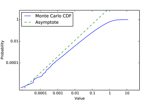
Figure 1: Left tail of the distribution function of the portfolio of three call options in a multidimensional Black-Scholes model.

Comparison with hidden regular variation

When assets and options are identical, the left tail behavior of a portfolio of options in the multidimensional Black-Scholes model can also be analyzed using hidden regular variation. For the purposes of this illustration, assume that the portfolio contains two options ($n=2$), leaving the general case for further research. Let $Z_{i}=-1/\ln\{1-\mathcal{N}(\tilde{X}_{i})\}$ for $i=1,2$. It is known (Weller and Cooley, 2014, page 6) that for all $z_{1},z_{2}>0$,

$$t\Pr\Big{[}\frac{Z_{1}}{b_{0}(t)}>z_{1},\frac{Z_{2}}{b_{0}(t)}>z_{2}\Big{]}\to(z_{1}z_{2})^{-\frac{1}{2\eta}}\quad\text{as $t\to\infty$}$$

where $\eta=(1+\rho)/{2}$ and $b_{0}(t)=U^{-1}(t)$ with

$$U(t)=t^{1/\eta}L_{0}(t),\quad L_{0}(t)=(1+\rho)^{3/2}(1-\rho)^{-1/2}(4\pi\ln t)^{-\rho/(1+\rho)}.$$ (12)

For all $x_{1},x_{2}>0$,

$$\Pr[P_{1}^{-1}>tx_{1},P_{2}^{-1}(tx_{2})]=\Pr[Z_{1}>g_{1}(tx_{1}),Z_{2}>g_{2}(tx_{2})],$$

where for $i=1,2$,

$$g_{i}(t)=-\frac{1}{\ln\left[1-\mathcal{N}\left\{f_{i}^{-1}\left(\frac{1}{t}\right)\right\}\right]}.$$

As $t\to\infty$, clearly,

$$g_{i}(t)\sim\tilde{g}_{i}(t):=\frac{1}{\mathcal{N}\left\{f_{i}^{-1}\left(\frac{1}{t}\right)\right\}}.$$

Moreover, using the equivalent (11), and the asymptotic expansion for $\mathcal{N}^{-1}$ given, e.g., in (Blair et al., 1976, page 828), it is easy to show that

$$\tilde{g}_{i}^{-1}(u)=\frac{1}{f_{i}\{\mathcal{N}^{-1}(1/u)\}}\sim C_{i}u^{\frac{T}{T_{i}-T}}(\ln u)^{1-\frac{T}{2(T_{i}-T)}}e^{-c_{i}\sqrt{\frac{2T}{T_{i}-T}\ln u}}$$

where

$$C_{i}=\frac{2T\sqrt{2\pi}}{\sigma_{i}(T_{i}-T)^{3/2}}e^{\frac{c_{i}^{2}}{2}-k_{i}}(2\sqrt{\pi})^{\frac{T}{T_{i}-T}}\quad\text{and}\quad c_{i}=\frac{\mu_{i}T+k_{i}}{\sigma_{i}\sqrt{T_{i}-T}}+\frac{\sigma_{i}\sqrt{T_{i}-T}}{2}.$$

In other words,

$$\tilde{g}_{i}^{-1}(u)=u^{\frac{T}{T_{i}-T}}L_{i}(u),$$

where $L_{i}$ is a slowly varying function as $u\to\infty$. It follows that

$$\tilde{g}_{i}(t)=t^{\frac{T_{i}-T}{T}}\tilde{L}_{i}(t),$$

where $\tilde{L}_{i}$ is slowly varying as $t\to\infty$. By asymptotic inversion we can show that $\tilde{L}_{i}$ satisfies the following relationship.

$$\tilde{L}_{i}(t)\sim C_{i}^{-\frac{T_{i}-T}{T}}\left(\frac{T_{i}-T}{T}\ln t\right)^{\frac{1}{2}-\frac{T_{i}-T}{T}}e^{c_{i}\frac{T_{i}-T}{T}\sqrt{2\ln t}},\quad t\to\infty.$$ (13)

Now assume that the options and the assets are identical so that $T_{1}=T_{2}$, $\tilde{L}_{1}=\tilde{L}_{2}:=\tilde{L}$ and $\tilde{g}_{1}=\tilde{g}_{2}:=\tilde{g}$. Then,

$$\Pr[P_{1}^{-1}>tx_{1},P_{2}^{-1}(tx_{2})]\sim\frac{(x_{1}x_{2})^{-\frac{T_{1}-T}{2\eta T}}}{U\{\tilde{g}(t)\}}.$$

Therefore, we conclude that the couple $(P_{1}^{-1},P_{2}^{-1})$ possesses the hidden regular variation property, and consequently

$$\Pr[P_{1}+P_{2}\leq z]=\Pr[(P_{1}^{-1},P_{2}^{-1})\in\frac{1}{z}A]\sim\frac{1}{U\{\tilde{g}(1/z)\}}\nu_{0}(A),$$

where

$$A=\{x>0,y>0:\frac{1}{x}+\frac{1}{y}\leq 1\}$$

and $\nu_{0}$ is a measure defined by

$$\nu_{0}((x_{1},\infty)\times(x_{2},\infty))=(x_{1}x_{2})^{-\frac{T_{1}-T}{2\eta T}}.$$

An easy computation shows that

$$\nu_{0}(A)=\gamma B(1+\gamma,2+\gamma),$$

where $B$ is the Euler beta function and

$$\gamma=\frac{T_{1}-T}{2\eta T}.$$

Finally, we have shown that as $z\to 0$,

$$\Pr[P_{1}+P_{2}\leq z]\sim z^{\frac{T_{1}-T}{\eta T}}\frac{\gamma B(1+\gamma,2+\gamma)}{\tilde{L}(1/z)^{1/\eta}L_{0}(z^{\frac{T-T_{1}}{T}})},$$

where the function $L_{0}$ is given explicitly in (12) and the function $\tilde{L}$ satisfies the asymptotic relation (13).

It is easy to see that in this case,

$$\inf_{\boldsymbol{w}\in\Delta_{n}}\boldsymbol{w}^{\top}\Sigma\boldsymbol{w}=\frac{\eta T}{T_{1}-T},$$

so that the leading term of the above formula agrees with Proposition 5. In conclusion, in this example, the hidden regular variation theory allows to compute the sharp asymptotics under a rather restrictive assumption of homogeneous portfolio, while the methodology of this paper is applicable in the general case but only enables us to compute the log scale asymptotics.

References

- Bingham et al. (1989) Bingham, N. H., C. M. Goldie, and J. L. Teugels (1989). Regular variation, Volume 27. Cambridge University Press.
- Black and Scholes (1973) Black, F. and M. Scholes (1973). The pricing of options and corporate liabilities. Journal of Political Economy 3, 637–654.
- Blair et al. (1976) Blair, J., C. Edwards, and J. Johnson (1976). Rational Chebyshev approximations for the inverse of the error function. Mathematics of Computation 30(136), 827–830.
- Coles et al. (1999) Coles, S., J. Heffernan, and J. Tawn (1999). Dependence measures for extreme value analyses. Extremes 2(4), 339–365.
- Das et al. (2013) Das, B., A. Mitra, S. Resnick, et al. (2013). Living on the multidimensional edge: seeking hidden risks using regular variation. Advances in Applied Probability 45(1), 139–163.
- De Haan and De Ronde (1998) De Haan, L. and J. De Ronde (1998). Sea and wind: multivariate extremes at work. Extremes 1(1), 7–45.
- De Haan and Ferreira (2007) De Haan, L. and A. Ferreira (2007). Extreme value theory: an introduction. Springer.
- Draisma et al. (2004) Draisma, G., H. Dress, A. Ferreira, and L. De Haan (2004). Bivariate tail estimation: dependence in asymptotic independence. Bernoulli 10(2), 251–280.
- Genest and Rivest (1989) Genest, C. and L.-P. Rivest (1989). A characterization of Gumbel’s family of extreme value distributions. Statistics & Probability Letters 8(3), 207–211.
- Gulisashvili and Tankov (2014) Gulisashvili, A. and P. Tankov (2015). Implied volatility of basket options at extreme strikes. In: Large Deviations and Asymptotic Methods in Finance, Friz, P., J. Gatheral, A. Gulisashvili, A. Jacqier, A. and J. Teichmann (eds.), Springer.
- Hashorva (2010) Hashorva, E. (2010). On the residual dependence index of elliptical distributions. Statistics & Probability Letters 80(13), 1070–1078.
- Hashorva and Hüsler (2003) Hashorva, E. and J. Hüsler (2003). On multivariate Gaussian tails. Annals of the Institute of Statistical Mathematics 55(3), 507–522.
- Heffernan et al. (2005) Heffernan, J., S. Resnick, et al. (2005). Hidden regular variation and the rank transform. Advances in Applied Probability 37(2), 393–414.
- Heffernan (2000) Heffernan, J. E. (2000). A directory of coefficients of tail dependence. Extremes 3(3), 279–290.
- Hult and Lindskog (2002) Hult, H. and F. Lindskog (2002). Multivariate extremes, aggregation and dependence in elliptical distributions. Advances in Applied probability 34(3), 587–608.
- Joe et al. (2010) Joe, H., H. Li, and A. K. Nikoloulopoulos (2010). Tail dependence functions and vine copulas. Journal of Multivariate Analysis 101(1), 252–270.
- Klüppelberg et al. (2008) Klüppelberg, C., G. Kuhn, and L. Peng (2008). Semi-parametric models for the multivariate tail dependence function–the asymptotically dependent case. Scandinavian Journal of Statistics 35(4), 701–718.
- Klüppelberg et al. (2007) Klüppelberg, C., G. Kuhn, L. Peng, et al. (2007). Estimating the tail dependence function of an elliptical distribution. Bernoulli 13(1), 229–251.
- Ledford and Tawn (1996) Ledford, A. W. and J. A. Tawn (1996). Statistics for near independence in multivariate extreme values. Biometrika 83(1), 169–187.
- Ledford and Tawn (1997) Ledford, A. W. and J. A. Tawn (1997). Modelling dependence within joint tail regions. Journal of the Royal Statistical Society: Series B (Statistical Methodology) 59(2), 475–499.
- Maulik and Resnick (2004) Maulik, K. and S. Resnick (2004). Characterizations and examples of hidden regular variation. Extremes 7(1), 31–67.
- Maulik et al. (2002) Maulik, K., S. Resnick, H. Rootzén, et al. (2002). Asymptotic independence and a network traffic model. Journal of Applied Probability 39(4), 671–699.
- McNeil et al. (2010) McNeil, A. J., R. Frey, and P. Embrechts (2010). Quantitative risk management: concepts, techniques, and tools. Princeton University Press.
- Nelsen (1999) Nelsen, R. (1999). An Introduction to Copulas. Springer.
- Resnick (2002) Resnick, S. (2002). Hidden regular variation, second order regular variation and asymptotic independence. Extremes 5(4), 303–336.
- Resnick (2007) Resnick, S. I. (2007). Heavy-tail phenomena: probabilistic and statistical modeling. Springer.
- Schlueter and Fischer (2012) Schlueter, S. and M. Fischer (2012). The weak tail dependence coefficient of the elliptical generalized hyperbolic distribution. Extremes 15(2), 159–174.
- Sibuya (1959) Sibuya, M. (1959). Bivariate extreme statistics, I. Annals of the Institute of Statistical Mathematics 11(2), 195–210.
- Weller and Cooley (2014) Weller, G. B. and D. Cooley (2014). A sum characterization of hidden regular variation with likelihood inference via expectation-maximization. Biometrika, to appear.