Solar wind protons at 1 AU: trends and bounds, constraints and correlations

Abstract

The proton temperature anisotropy in the solar wind exhibits apparent bounds which are compatible with the theoretical constraints imposed by temperature-anisotropy driven kinetic instabilities. Recent statistical analyses based on conditional averaging indicate that near these theoretical constraints the solar wind protons have typically enhanced temperatures and a weaker collisionality. Here we carefully analyze the solar wind data and show that these results are a consequence of superposition of multiple correlations in the solar wind, namely, they mostly result from the correlation between the proton temperature and the solar wind velocity and from the superimposed anti-correlation between the proton temperature anisotropy and the proton parallel beta in the fast solar wind. Colder and more collisional data are distributed around temperature isotropy whereas hotter and less collisional data have a wider range of the temperature anisotropy anti-correlated with the proton parallel beta with signatures of constraints owing to the temperature-anisotropy driven instabilities. However, most of the hot and weakly collisional data, including the hottest and least collisional ones, lies far from the marginal stability regions. Consequently, we conclude that there is no clear relation between the enhanced temperatures and instability constraints and that the conditional averaging used for these analyses must be used carefully and need to be well tested.

I. Introduction

Physical mechanisms responsible for acceleration and heating of the solar wind plasma still remain to a large extent an open problem (Hollweg, 2008; Matthaeus & Velli, 2011; Hellinger et al., 2013). Different processes leave imprints in the solar wind particle properties and may be thus possibly identified (Marsch, 2012; Matteini et al., 2012). The solar wind protons at 1 AU exhibit many different correlations and apparent bounds which are not fully understood. The proton temperature $T_{\mathrm{p}}$ is correlated with the solar wind velocity $v_{sw}$ (Matthaeus et al., 2006; Démoulin, 2009; Elliott et al., 2012) whereas the proton number density $n_{\mathrm{p}}$ is anti-correlated with $v_{sw}$. The proton parallel beta $\beta_{\mathrm{p}\|}=2\mu_{0}n_{\mathrm{p}}k_{B}T_{\mathrm{p}\|}/B_{0}^{2}$ (the ratio between the proton parallel pressure and the magnetic pressure) and the proton temperature anisotropy $\mathcal{A}_{\mathrm{p}}=T_{\mathrm{p}\perp}/T_{\mathrm{p}\|}$ are anti-correlated in the fast solar wind (Marsch et al., 2004; Hellinger et al., 2006) as

$$\mathcal{A}_{\mathrm{p}}\sim 1.16\beta_{\mathrm{p}\parallel}^{-0.55}.$$ (1)

Moreover, $\beta_{\mathrm{p}\|}$ increases and $\mathcal{A}_{\mathrm{p}}$ decreases with the radial distance between 0.3 and 1 AU following the trend of Eq. (1) in the fast solar wind (Matteini et al., 2007). Here $T_{\mathrm{p}\|}$ and $T_{\mathrm{p}\perp}$ are the proton parallel and perpendicular temperatures (with respect to the ambient magnetic field), respectively, $B_{0}$ is the magnitude of the ambient magnetic field, $\mu_{0}$ and $k_{B}$ are the magnetic permeability and the Botzmann constant, respectively.

Coulomb collisions are typically too weak to keep the plasma in thermal equilibrium and the solar wind protons exhibit important particle temperature anisotropies. The proton temperature anisotropy $\mathcal{A}_{\mathrm{p}}$, however, seems to be constrained. The data distribution in the $(\beta_{\mathrm{p}\|},\mathcal{A}_{\mathrm{p}})$ space has roughly a rhomboidal shape and the apparent bounds on the high $\beta_{\mathrm{p}\|}$ side are compatible with the theoretical constraints imposed by kinetic instabilities driven by the proton temperature anisotropy (Kasper et al., 2002; Hellinger et al., 2006).

Important solar wind parameters (such as the collisional time, the proton temperature, and the amplitude of the turbulent/fluctuating magnetic field) seem to be related to kinetic instabilities. Some statistical studies indicate that these physical quantities are enhanced or reduced near marginal stability regions of the temperature-anisotropy driven instabilities (Bale et al., 2009; Maruca et al., 2011; Osman et al., 2012; Wicks et al., 2013). This may indicate a connection between these kinetic instabilities and processes which are likely responsible for the proton heating such as the magnetohydrodynamic turbulence (Matthaeus & Velli, 2011; Osman et al., 2013). However, these studies are based on a conditional averaging: the data are split in bins in the 2-D space of $\beta_{\mathrm{p}\|}$ and $\mathcal{A}_{\mathrm{p}}$ with variable sizes and number of points and an averaging within the different bins is used to get a dependence of a third physical parameter on $\beta_{\mathrm{p}\|}$ and $\mathcal{A}_{\mathrm{p}}$. This procedure is not trivial and its results need to be tested. In this letter we analyze in detail possible relations between the proton collisionality and temperature, and $\beta_{\mathrm{p}\|}$ and $\mathcal{A}_{\mathrm{p}}$. In particular we demonstrate that the reported enhancements of the proton temperature near marginal stability regions (resulting from the bin-averaged procedure) are related to the structure of the data distribution in the ($\beta_{\mathrm{p}\|}$, $\mathcal{A}_{\mathrm{p}}$, $T_{\mathrm{p}}$) space.

II. Data analysis

Here we use a large statistical data set (about 4 millions data points) from the WIND spacecraft from 1995 to 2012 (Maruca et al., 2012). Let us first investigate a possible relation between $\beta_{p\|}$ and $\mathcal{A}_{\mathrm{p}}$, and the proton collisionality characterized by the collisional time $\tau=\nu_{T}t_{e}$ (a proxy for the collisional age) where $t_{e}=1\ \mathrm{AU}/v_{sw}$ is the expansion (transit) time and $\nu_{T}$ is the collisional proton isotropization frequency defined as

$$\left[\frac{\mathrm{d}(T_{\mathrm{p}\perp}-T_{\mathrm{p}\|})}{\mathrm{d}t}\right]_{collisions}=-\nu_{T}(T_{\mathrm{p}\perp}-T_{\mathrm{p}\|});$$ (2)

$\nu_{T}$ may be derived assuming a bi-Maxwellian velocity distribution function and expressed in terms of the standard Gauss hypergeometric function $\ {}_{2}F_{1}$ as (Hellinger & Trávníček, 2009, 2010)

$$\nu_{T}=\frac{e^{4}n_{\mathrm{p}}\ln\Lambda}{30\pi^{3/2}\varepsilon_{0}^{2}\sqrt{m_{\mathrm{p}}k_{B}^{3}T_{\mathrm{p}\|}^{3}}}\ _{2}F_{1}\left(2,\frac{3}{2};\frac{7}{2};1-\mathcal{A}_{\mathrm{p}}\right),$$ (3)

where $e$ is the proton charge, $\ln\Lambda$ is the Coulomb logarithm, $\varepsilon_{0}$ is the permittivity of vacuum, and $m_{\mathrm{p}}$ is the proton mass. These four parameters are not however independent, they depend on the proton (parallel) temperature; if we neglect the role of other parameters we get

$$\mathcal{A}_{\mathrm{p}}\propto 1/\beta_{p\|}\ \ \textrm{and}\ \ \tau\propto T_{\mathrm{p}}^{-3/2}.$$ (4)

These interdependencies need to be taken in account when interpreting the observations; note that while Eq. (4) predicts an anti-correlation between $\mathcal{A}_{\mathrm{p}}$ and $\beta_{p\|}$ it is not sufficient to explain quantitatively the observed anti-correlation of Eq. (1).

A natural way to investigate a relation between three physical quantities would be a three-dimensional frequency plot/histogram. Such three dimensional plots are however hard to visualize and interpret so that we use here only two-dimensional analyses. In this way, the connections between the parameters due to interdependences such as in Eq. (4) may be discern. The relation between the proton $\beta_{\mathrm{p}\|}$, the proton temperature anisotropy $\mathcal{A}_{\mathrm{p}}$ and the collisional time $\tau$ is investigated in Figure 1. The left top panel shows a color scale plot of the observed relative frequency (normalized to the bin size (Maruca et al., 2012)) of ($\beta_{\mathrm{p}\|}$, $\tau$), the right top panel shows a similar plot for ($\mathcal{A}_{\mathrm{p}}$, $\tau$), and the left bottom panel displays the case of ($\beta_{\mathrm{p}\|}$,$\mathcal{A}_{\mathrm{p}}$).

The right bottom panel shows the bin-averaged collisional time $\tau$ as a function of $\beta_{\mathrm{p}\|}$ and $\mathcal{A}_{\mathrm{p}}$ (Bale et al., 2009): for a given bin in $\beta_{\mathrm{p}\|}$ and $\mathcal{A}_{\mathrm{p}}$ the average collisional time $\tau$ is calculated and the result is plotted as $\tau=\tau(\beta_{\mathrm{p}\|},\mathcal{A}_{\mathrm{p}})$. Note that different bins have different sizes and different “weights”, i.e., different number of data points used for averaging. Here we show results only for bins with more than 20 data points.

The bottom left panel shows the data distributed in the ($\beta_{\mathrm{p}\|}$,$\mathcal{A}_{\mathrm{p}}$) space which is useful for the electromagnetic temperature-anisotropy driven instabilities; the different overplotted curves (solid one for the proton cyclotron instability, dotted one for the mirror instability, dashed one for the parallel fire hose, and the dash-dotted one for the oblique fire hose) denote the marginal stability relations, i.e., where the corresponding bi-Maxwellian linear kinetic theory predicts that the fastest growing mode has the growth rate $\gamma_{\mathrm{max}}(\beta_{\mathrm{p}\|},\mathcal{A}_{\mathrm{p}})=10^{-3}\omega_{c\mathrm{p}}$ (where $\omega_{c\mathrm{p}}$ is the proton cyclotron frequency) (Hellinger et al., 2006). The system becomes more unstable when increasing $\beta_{\mathrm{p}\|}$ and/or when increasing (decreasing) $\mathcal{A}_{\mathrm{p}}$ for $\mathcal{A}_{\mathrm{p}}>1$ (for $\mathcal{A}_{\mathrm{p}}<1$). The data exhibit bounds which are more compatible with theoretical constraints imposed by the weaker, oblique instabilities (mirror and oblique fire hose) apparently at odds with the expected important role of the linearly dominant instabilities (proton cyclotron and parallel fire hose); however, the theoretical prediction is based on simplified and idealized plasma composition and properties (Matteini et al., 2012) and, moreover, these instabilities are resonant, i.e., their stability strongly depends on a detailed structure of the particle velocity distribution function (Hellinger & Trávníček, 2011; Isenberg et al., 2013).

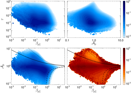
Figure 1.— The left top panel shows a color scale plot of the observed relative frequency of ($\beta_{\mathrm{p}\|}$, $\tau$), the right top panel shows a similar plot for ($\mathcal{A}_{\mathrm{p}}$, $\tau$), and the left bottom panel displays the case of ($\beta_{\mathrm{p}\|}$,$\mathcal{A}_{\mathrm{p}}$). The right bottom panel shows the bin-averaged $\tau=\tau(\beta_{\mathrm{p}\|},\mathcal{A}_{\mathrm{p}})$. The overplotted curves on the bottom panels show the marginal stability relations ($\gamma_{max}=10^{-3}\omega_{c\mathrm{p}}$) for the (solid) proton cyclotron (dotted) mirror, (dashed) parallel fire hose, and (dash-dotted) oblique fire hose instabilities.

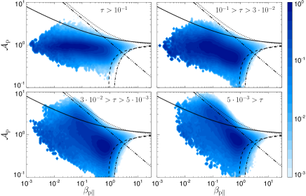
Figure 2.— Color scale plots of the relative frequency of ($\beta_{\mathrm{p}\|}$,$\mathcal{A}_{\mathrm{p}}$) for different ranges of collisional time (top left) $\tau>10^{-1}$, (top right) $10^{-1}>\tau>3\cdot 10^{-2}$, (bottom left), $3\cdot 10^{-2}>\tau>5\cdot 10^{-3}$, and (bottom right) $\tau<5\cdot 10^{-3}$. The overplotted curves show the marginal stability relations as in Fig. 1 whereas the dash-dot-dot-doted line displays the anti-correlation (1).

Figure 1 demonstrates that there is no clear relation between the collisional time $\tau$ and $\beta_{\mathrm{p}\|}$ (top left) whereas for larger $\tau$ the proton temperature anisotropy $\mathcal{A}_{\mathrm{p}}$ is weaker and approaches $\mathcal{A}_{\mathrm{p}}\sim 1$ for very large $\tau$ (top right). The bottom right panel indicates that the data around temperature isotropy $\mathcal{A}_{\mathrm{p}}\sim 1$ are on average more collisional whereas the data near the marginal stability regions are less collisional (Bale et al., 2009).

To understand this behavior we now analyze the relation between $\tau$, $\beta_{\mathrm{p}\|}$, and $\mathcal{A}_{\mathrm{p}}$ in more detail. Figure 2 shows color scale plots of the relative frequency of ($\beta_{\mathrm{p}\|}$, $\mathcal{A}_{\mathrm{p}}$) for different ranges of collisional times from more to less collisional plasmas (from left to right and from top to bottom). Each range of $\tau$ has about the same number of points (1 million). The dash-dot-dot-doted line displays Eq. (1). We observe that the most collisional protons exhibit a distribution centered around temperature isotropy $\mathcal{A}_{\mathrm{p}}\sim 1$ with a large variation of $\beta_{\mathrm{p}\|}$. This distribution gradually transforms to an anti-correlation between $\beta_{\mathrm{p}\|}$ and $\mathcal{A}_{\mathrm{p}}$ with varying slopes. For the lowest collisional times the anti-correlation becomes comparable to Eq. (1) (Hellinger et al., 2006; Matteini et al., 2007). Figure 2 gives a clear explanation of the bottom right panel of Fig. 1. The more collisional data contribute to the bin averages more around $\mathcal{A}_{\mathrm{p}}\sim 1$ (for lower $\beta_{\mathrm{p}\|}$) whereas the less collisional data contribute more around the anti-correlation (and further away from the isotropic region). Figure 1 then indicates lower average collisional time near marginal stability regions as a result of the bin averaging, but the more detailed analysis of Fig. 2 does not show any clear relation between the reduced collisional age and marginal stabilities; weakly collisional data are bounded by the marginal stability regions but most of them lie far from them in vicinity of temperature isotropy.

It is also noteworthy that the data distribution in Fig. 2 extends to lower $\beta_{\mathrm{p}\|}$ (and more isotropic $\mathcal{A}_{\mathrm{p}}$) for more collisional plasmas. The apparent bounds on the left hand side (Fig. 1, bottom left, for low $\beta_{\mathrm{p}\|}$) of the data distribution in ($\beta_{\mathrm{p}\|}$, $\mathcal{A}_{\mathrm{p}}$) are therefore likely a consequence of (proton-proton) Coulomb collisions.

The proton temperature $T_{\mathrm{p}}$ exhibits similar (but opposite) behavior with respect to the marginal stability regions in the $(\beta_{\mathrm{p}\|},\mathcal{A}_{\mathrm{p}})$ space compared to $\tau$ as expected from Eq. (4. $T_{\mathrm{p}}$ seems to be enhanced near the marginal stability regions (Maruca et al., 2011). Let us now apply a similar analysis to the relation between $\beta_{\mathrm{p}\|}$, $\mathcal{A}_{\mathrm{p}}$ and $T_{\mathrm{p}}$. Figure 3 shows color scale plots of the observed relative frequency of ($\beta_{\mathrm{p}\|}$, $T_{\mathrm{p}}$) (top left), of ($\mathcal{A}_{\mathrm{p}}$, $T_{\mathrm{p}}$) (top right), and of ($\beta_{\mathrm{p}\|}$,$\mathcal{A}_{\mathrm{p}}$) (bottom left). The right bottom panel shows the bin-averaged proton temperature $T_{\mathrm{p}}$ as a function of $\beta_{\mathrm{p}\|}$ and $\mathcal{A}_{\mathrm{p}}$. (only bins with more than 20 data points are shown).

The proton temperature $T_{\mathrm{p}}$ indeed seems to be enhanced near the marginal stability regions. Let us now look in more detail at the relation between the proton temperature and the $(\beta_{\mathrm{p}\|},\mathcal{A}_{\mathrm{p}})$ space. Figure 4 shows color scale plots of the relative frequency of ($\beta_{\mathrm{p}\|}$, $\mathcal{A}_{\mathrm{p}}$) for different ranges of the proton temperature from hotter to colder protons (from left to right and from top to bottom). Each range of $T_{\mathrm{p}}$ has about the same number of points (1 million). These partial data distributions have clearly opposite behavior compared to that of the collisional time (Fig. 2). For the hottest protons the data distribution exhibit an anti-correlation similar to Eq. (1) which gradually transforms (anti-correlations with a decreasing slope) to a distribution centered around temperature isotropy with a wide range of $\beta_{\mathrm{p}\|}$ for the coldest protons. Again, Figure 4 gives a clear explanation of the bottom right panel of Fig. 3. Colder, more collisional protons contribute importantly around temperature isotropy whereas hotter, less collisional protons contribute more around the anti-correlation between $\beta_{\mathrm{p}\|}$ and $\mathcal{A}_{\mathrm{p}}$. As a result of the bin-averaging procedure the proton temperature seems to be enhanced near marginal stability regions (and for important temperature anisotropies). However, no clear relation between the enhanced proton temperature and marginal stabilities is found; hotter proton data are bounded by the marginal stability regions but most of them lie far from them in vicinity of temperature isotropy.

The presented analysis divided the data in subsets (with about the same sizes) according to the proton collisional age or temperature. This approach misses smaller scale structure of the data. In order to test whether we don’t loose important properties we repeated the analysis by splitting the data in $\tau$ and $T_{\mathrm{p}}$ in 8 and also 16 subsets with about the same sizes and we recovered essentially the same behavior, the transition from colder, collisional data distributed around temperature isotropy to hot, less collisional data exhibiting an anti-correlation between $\beta_{\mathrm{p}\|}$ and $\mathcal{A}_{\mathrm{p}}$. In each case even the hottest (and the least collisional) proton data are bounded by the marginal stability regions but most of them lie far from them in vicinity of temperature isotropy.

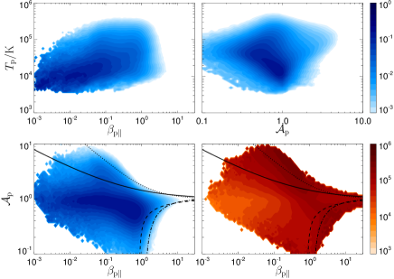
Figure 3.— The left top panel shows a color scale plot of the observed relative frequency of ($\beta_{\mathrm{p}\|}$, $T_{\mathrm{p}}$), the right top panel shows a similar plot for ($\mathcal{A}_{\mathrm{p}}$, $T_{\mathrm{p}}$), and the left bottom panel displays the case of ($\beta_{\mathrm{p}\|}$, $\mathcal{A}_{\mathrm{p}}$). The right bottom panel shows the bin-averaged $T_{\mathrm{p}}=T_{\mathrm{p}}(\beta_{\mathrm{p}\|},\mathcal{A}_{\mathrm{p}})$. The overplotted curves on the bottom panels show the marginal stability relations as in Fig. 1.

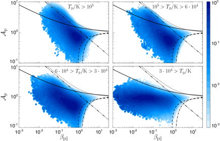
Figure 4.— Color scale plots of the relative frequency of ($\beta_{\mathrm{p}\|}$, $\mathcal{A}_{\mathrm{p}}$) for (top left) $T_{\mathrm{p}}/\mathrm{K}>10^{5}$, (top right) $10^{5}>T_{\mathrm{p}}/\mathrm{K}>6\cdot 10^{4}$, (bottom left) $6\cdot 10^{4}>T_{\mathrm{p}}/\mathrm{K}>3\cdot 10^{4}$, and (bottom right) $3\cdot 10^{4}>T_{\mathrm{p}}/\mathrm{K}$. The overplotted curves show the marginal stability relations as in Fig. 1 whereas the dash-dot-dot-doted line displays the anti-correlation (1).

The proton temperature and the collisional time have clear opposite behaviors indicating an anti-correlation between them. Such an anti-correlation is expected from Eq. (4) and, moreover, the proton temperature correlates with the solar wind velocity $v_{sw}$ which in turn anti-correlates with the proton density. Figure 5 confirms this property, it shows on the left panel the relative frequency of ($v_{sw}$, $T_{\mathrm{p}}$) and that of ($\tau$, $T_{\mathrm{p}}$) on the right panel. The relation between $v_{sw}$ and $T_{\mathrm{p}}$ is roughly linear

$$T_{\mathrm{p}}/\mathrm{K}=-1.6\cdot 10^{5}+590\times v_{sw}/(\mathrm{km/s})$$ (5)

(shown by the solid line on Fig. 5, left) and it is similar to the trend observed by (Elliott et al., 2012). The relation between the collisional time $\tau$ and $T_{\mathrm{p}}$ is well described by

$$T_{\mathrm{p}}/\mathrm{K}=1.1\cdot 10^{4}\tau^{-0.46}$$ (6)

(shown by the solid line on Fig. 5, right). The anti-correlation of Eq. (6) cannot be explained only by Eq. (4); taking $T_{\mathrm{p}}\propto v_{sw}$ (roughly Eq. (5)) one gets $T_{\mathrm{p}}\propto\tau^{-2/5}$ which is close to the observed Eq. (6).

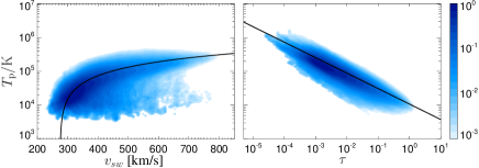
Figure 5.— Color scale plots of the relative frequency of ($v_{sw}$, $T_{\mathrm{p}}$) (left panel) and of ($\tau$, $T_{\mathrm{p}}$) (right panel). Overplotted curves show Eq. (5) and Eq. (6).

III. Discussion

The solar wind protons exhibit many not-yet-fully-understood correlations. The proton temperature $T_{\mathrm{p}}$ is correlated with the solar wind velocity $v_{sw}$, the collisional time $\tau$ is well anti-correlated with $T_{\mathrm{p}}$, and the proton parallel beta $\beta_{\mathrm{p}\|}$ and the proton temperature anisotropy $\mathcal{A}_{\mathrm{p}}$ are anti-correlated in the fast solar wind.

The bin-averaging procedure produces plots as $\tau=\tau(\beta_{\mathrm{p}\|},\mathcal{A}_{\mathrm{p}})$ and $T_{\mathrm{p}}=T_{\mathrm{p}}(\beta_{\mathrm{p}\|},\mathcal{A}_{\mathrm{p}})$ (see Figs. 2 and 4, bottom right) which indicate a connection between the marginal stability regions of kinetic instabilities and the collisional time or the proton temperature (Bale et al., 2009; Maruca et al., 2011). One of the problems of the bin averaging is that it combines averages over highly variable bin and data sizes. This effect may in some cases help to discern some trends. However, here we show that reduced $\tau$ and enhanced $T_{\mathrm{p}}$ near the marginal stability regions rather reflects the data structure in the corresponding three-dimensional space connected with the multiple correlations in the solar wind; there is no statistically significant number of data points with reduced $\tau$ and enhanced $T_{\mathrm{p}}$ near the marginal stability regions. Colder and more collisional data are distributed around temperature isotropy whereas hotter and less collisional data have a wider spread in the space $(\beta_{\mathrm{p}\|},\mathcal{A}_{\mathrm{p}})$ reaching the marginal stability regions; however, most of the hot and weakly collisional data (including the hottest and least collisional ones) lie far from the marginal stability regions. We conclude that the bin-averaging method is a nontrivial procedure which should be carefully used and its results must be tested in detail which is not usually done. Some previous studies where this method has been applied (Kasper et al., 2008; Bale et al., 2009; Osman et al., 2012; Kasper et al., 2013; Wicks et al., 2013; Osman et al., 2013; Bourouaine et al., 2013; Servidio et al., 2014) likely need to be revisited. In particular, the fluctuating magnetic field $\delta B$ (3 second r.m.s.) dependence on $\beta_{\mathrm{p}\|}$ and $\mathcal{A}_{\mathrm{p}}$ (obtained through the bin-averaging method) exhibits enhancements of $\delta B$ near the marginal stability regions similarly to the proton temperature (Bale et al., 2009). However, the 3 second r.m.s. $\delta B$ is clearly anti-correlated with the collisional time (see Fig. 3 of Bale et al., 2009) so that we expect that the enhancements of $\delta B$ are to some extent a consequence of this anti-correlation. On the other hand, Wicks et al. (2013) used Ulysses data to show (using the bin-averaging method) that the fluctuating magnetic field on ion scales is enhanced near the marginal stability regions. This analysis used only data from the fast solar wind and therefore the influence of the correlation between the solar wind velocity and the level of magnetic fluctuations is likely negligible in this case. Further studies are needed to understand origins and consequences of multiple correlations in the solar wind.

References

- Bale et al. (2009) Bale, S. D., Kasper, J. C., Howes, G. G., Quataert, E., Salem, C., & Sundkvist, D. 2009, Phys. Rev. Lett., 103, 211101
- Bourouaine et al. (2013) Bourouaine, S., Verscharen, D., Chandran, B. D. G., Maruca, B. A., & Kasper, J. C. 2013, ApJL, 777, L3
- Démoulin (2009) Démoulin, P. 2009, Sol. Phys., 257, 169
- Elliott et al. (2012) Elliott, H. A., Henney, C. J., McComas, D. J., Smith, C. W., & Vasquez, B. J. 2012, J. Geophys. Res., 117, A09102
- Hellinger et al. (2006) Hellinger, P., Trávníček, P., Kasper, J. C., & Lazarus, A. J. 2006, Geophys. Res. Lett., 33, L09101
- Hellinger & Trávníček (2009) Hellinger, P., & Trávníček, P. M. 2009, Phys. Plasmas, 16, 054501
- Hellinger & Trávníček (2010) —. 2010, J. Comput. Phys., 229, 5432
- Hellinger & Trávníček (2011) —. 2011, J. Geophys. Res., 116, A11101
- Hellinger et al. (2013) Hellinger, P., Trávníček, P. M., Štverák, Š., Matteini, L., & Velli, M. 2013, J. Geophys. Res., 118, 1351
- Hollweg (2008) Hollweg, J. V. 2008, J. Astrophys. Astron., 29, 217
- Isenberg et al. (2013) Isenberg, P. A., Maruca, B. A., & Kasper, J. C. 2013, ApJ, 773, 164
- Kasper et al. (2002) Kasper, J. C., Lazarus, A. J., & Gary, S. P. 2002, Geophys. Res. Lett., 29, 1839
- Kasper et al. (2008) —. 2008, Phys. Rev. Lett., 101, 261103
- Kasper et al. (2013) Kasper, J. C., Maruca, B. A., Stevens, M. L., & Zaslavsky, A. 2013, Phys. Rev. Lett., 110, 091102
- Marsch (2012) Marsch, E. 2012, Space Sci. Rev., 172, 23
- Marsch et al. (2004) Marsch, E., Ao, X.-Z., & Tu, C.-Y. 2004, J. Geophys. Res., 109, A04102
- Maruca et al. (2011) Maruca, B. A., Kasper, J. C., & Bale, S. D. 2011, Phys. Rev. Lett., 107, 201101
- Maruca et al. (2012) Maruca, B. A., Kasper, J. C., & Gary, S. P. 2012, ApJ, 748, 137
- Matteini et al. (2012) Matteini, L., Hellinger, P., Landi, S., Trávníček, P. M., & Velli, M. 2012, Space Sci. Rev., 172, 373
- Matteini et al. (2007) Matteini, L., Landi, S., Hellinger, P., Pantellini, F., Maksimovic, M., Velli, M., Goldstein, B. E., & Marsch, E. 2007, Geophys. Res. Lett., 34, L20105
- Matthaeus et al. (2006) Matthaeus, W. H., Elliott, H. A., & McComas, D. J. 2006, J. Geophys. Res., 111, A10103
- Matthaeus & Velli (2011) Matthaeus, W. H., & Velli, M. 2011, Space Sci. Rev., 160, 145
- Osman et al. (2012) Osman, K. T., Matthaeus, W. H., Hnat, B., & Chapman, S. C. 2012, Phys. Rev. Lett., 108, 261103
- Osman et al. (2013) Osman, K. T., Matthaeus, W. H., Kiyani, K. H., Hnat, B., & Chapman, S. C. 2013, Phys. Rev. Lett., 111, 201101
- Servidio et al. (2014) Servidio, S., Osman, K. T., Valentini, F., Perrone, D., Califano, F., Chapman, S., Matthaeus, W. M., & Veltri, P. 2014, ApJL, 781, L27
- Wicks et al. (2013) Wicks, R. T., Matteini, L., Horbury, T. S., Hellinger, P., & Roberts, A. D. 2013, in Proc. 13th Int. Solar Wind Conf., Vol. 1539 (AIP Conf. Proc.), 303–306