Abstract

We report on a bistable light transmission through a bilayer “fish-scale” (meander-line) metamaterial. It is demonstrated that an all-optical switching may be achieved nearly the frequency of the high-quality-factor Fano-shaped trapped-mode resonance excitation. The nonlinear interaction of two closely spaced trapped-mode resonances in the bilayer structure composed with a Kerr-type nonlinear dielectric slab is analyzed in both frequency and time domains. It is demonstrated that these two resonances react differently on the applied intense light which leads to destination of a multistable transmission.

OCIS codes: 190.1450, 160.3918, 230.1150, 230.4320.

1 Introduction

During recent years research efforts on both fundamental physics and applications of nonlinear optics demonstrate several major trends [1]. First, the basic concepts of nonlinear optics penetrated into new areas of material science by exploring novel nonlinear materials and nonlinear propagation of light in engineered structures. Second, there are a number of novel concepts related to tunable nonlinear response, and engineered and enhanced nonlinearities, which should be explored more extensively for developing advanced optical tunable nonlinear devices. Moreover, in such structures many of the effects well studied in nonlinear optics can be enhanced by the cavity effects, heterostructures, or Fano-type resonances, that enable much stronger nonlinear response at lower powers. Metamaterials based on planar resonant patterns are expected to become the key building blocks for such nonlinearity-enhanced effects and devices.

It is believed that the fabrication of metal-dielectric composite structures where the dielectric layers possess strong nonlinear response can allow the realization of tunable nonlinear metamaterials. The important area where the role of such nonlinear structures is expected to become more and more pronounced is the creation of all-optical circuitry for computing, information processing, and networking which is expected to overcome the speed limitations of electronics-based systems.

Typically metamaterials consist of arrays of magnetically or electrically polarizable elements. In many common configurations, the functional metamaterial inclusions are planar metallic patterns composed of symmetrical split-ring resonators (SRRs), on which currents are induced that flow in response to incident electromagnetic fields. A distinct property of metamaterials is that the capacitive regions of SRRs strongly confine and enhance the local electric field. The capacitive region of a metamaterial element thus provides a natural entry point at which some lumped frequency-dispersive, active, tunable or nonlinear materials can be introduced, providing a mechanism for coupling the metamaterial geometric resonance to other fundamental material properties [2, 3, 4]. The hybridization of metamaterials with semiconductors, ferromagnetic/ferrimagnetic materials and other externally tunable materials has already expanded the realm of metamaterials from the passive, linear media initially considered.

While the wave propagation can be controlled by using metamaterials with a unit cell consisting of a single resonant element (symmetrical split-ring resonator), other characteristics can also be controlled by using metamaterials composed of coupled resonators. Such metamaterials sometimes are also referred to EIT-like metamaterials [5, 6]. Typically they consist of identical subwavelength metallic inclusions structured in the form of asymmetrical split-rings (ASRs) [7, 8], split squares [9] or their complementary patterns [10]. These elements are arranged periodically and placed on a thin dielectric substrate. It is revealed that since these particles possess specific structural asymmetry, in a certain frequency band, the antiphase current oscillations with almost the same amplitudes appear on the particles parts (arcs). The scattered electromagnetic far-field produced by such current oscillations is very weak, which drastically reduces its coupling to free space and therefore radiation losses. Indeed, both the electric and magnetic dipole radiations of currents oscillating in the arcs of particles are canceled. As a consequence, the strength of the induced current can reach very high value and therefore ensure a high-$Q$ resonant optical response. Such a resonant regime is referred to so-called “trapped-modes”, since this term is traditionally used in describing electromagnetic modes which are weakly coupled to free space.

The features of nonlinear trapped-mode resonances were previously studied theoretically in planar metamaterials composed of asymmetrical split-rings [11] and two concentric rings [12, 13, 14]. In both configurations the substrate which carries the metallic pattern is considered as a nonlinear dielectric. The effect of nonlinearity appears as the formation of a closed loop of bistable transmission within the frequency of trapped-mode resonance. Since the nonlinear response of these metamaterials operating in the trapped-mode regime is extremely sensitive to the dielectric properties of the substrate it allows one to control switching operation effectively.

Another type of structures, which bears Fano-shaped trapped-mode resonances and is very promising for applications, is planar metamaterials consisted of equidistant array of continuous meander or zigzag metallic strips placed on a thin dielectric substrate (fish-scale structures [15, 16, 17]). In the past such structures have been investigated both theoretically [15, 19, 18, 20] and experimentally [15]. It is revealed, when the wave is polarized orthogonally to the strips, the fish-scale structure is transparent across a wide spectral range apart from an isolated wavelength. In contrary, when the wave is polarized parallel to the strips, it becomes a good broad-band reflector apart from an isolated wavelength where transmission is high. The same array combined with a homogeneous metallic mirror is also a good reflector which preserves a phase of the reflected wave with respect to the incident wave at this particular wavelength [15, 21]. The latter phenomenon is known as a “magnetic mirror” [22]. Finally, the structure also acts as a local field concentrator and a resonant multifold “amplifier” of losses in the constitutive dielectric.

Among others, a trapped-mode resonance can be excited in a fish-scale structure if the incident field is polarized along the strips and when the form of these strips is slightly different from the straight line. In such a system the less the form of strips is different from the straight line, the greater is the quality factor of the trapped-mode resonance. But, unfortunately, as the line curvature decreases, the resonant frequency shifts to the frequency where the Rayleigh anomaly occurs which diminishes the degree of the field localization within the system.

Nevertheless, in a bilayer configuration of the metamaterial, in which two equal gratings are adjusted to each side of a dielectric slab, it is possible to excite the high-$Q$ trapped-mode resonance far from the Rayleigh anomaly [19]. This resonance appears due to the oscillations of currents which flow in opposite directions relative to the adjacent gratings. In this case the electromagnetic field is strongly localized in the area between the adjacent gratings. Furthermore, in the bilayer structure, besides the trapped-mode resonance excited by gratings, some interference resonances appear in the similar manner as in traditional systems with gratings of straight lines. Therefore the bilayer fish-scale structure allows one to obtain different resonant features. The most important thing is that in the bilayer fish-scale structure the trapped-mode resonance has quality factor which is sufficiently greater than that ones attainable in the convenient interference resonances.

We should also note that the trapped-mode resonances can be excited in a very thin bilayer structure which is important for practical applications. We argue that the bilayer configuration is of a great interest in the case when the substrate is made of a field intensity dependent material (e.g. a Kerr-type medium) because the strong field localization between the gratings can significantly enhance the nonlinear effects. It leads to some particular manifestation of effects of bistability and multistability nearly the frequencies of Fano-shaped trapped-mode resonances which is presented in this paper.

2 Problem formulation

2.A Bilayer fish-scale metamaterial

A studied structure consists of two gratings of planar perfectly conducting infinite wavy-line strips placed on the both sides of a dielectric slab with thickness $h$ and permittivity $\varepsilon$ (see Fig. 1). The elementary translation (unit) cell of the structure under study is a square with sides $d=d_{x}=d_{y}$. The total length of the strip within the elementary translation cell is $S$. Suppose that the thickness $h$ and size $d$ are less then the wavelength $\lambda$ of the incident electromagnetic radiation ($h\ll\lambda$, $d<\lambda$). The width of the metal strips and their deviation from the straight line are $2w$ and $\Delta$, respectively.

Assume that the incident field is a plane monochromatic wave

$$\vec{E}^{inc}=\vec{p}A_{0}\exp(-i\vec{k}^{inc}\vec{r}),$$ (1)

where $\vec{p}$ is the unit vector which defines the polarization of the incident wave, $|p|=1$; $A_{0}$ and $\vec{k}^{inc}=\vec{e}_{x}k_{x}^{inc}+\vec{e}_{y}k_{y}^{inc}+\vec{e}_{z}k_{z}^{inc}$ are the magnitude and wavevector of the incident wave, respectively; $\vec{e}_{x}$, $\vec{e}_{y}$, $\vec{e}_{z}$ are orts of the coordinate system; $k^{inc}=k=\omega\sqrt{\varepsilon_{0}\mu_{0}}$. The time dependence is supposed to be $\exp(i\omega t)$.

In the frequency domain a solution of the diffraction problem on the bilayer structure is derived using the method of moments. It is formulated similarly to that one obtained for a single-layer metamaterial’s configuration [18, 19]. Farther the solution of the linear problem is used to construct a solution of the nonlinear problem.

We shall seek for the field through the entire space in the form of a superposition of the field without gratings $\vec{E}^{d}$ and the field scattered by gratings $\vec{E}^{s}$

$$\vec{E}=\vec{E}^{d}+\vec{E}^{s}.$$ (2)

Here $\vec{E}^{d}=\vec{E}^{inc}+\mathbb{\vec{R}}\exp(-i\vec{k}^{s}\vec{r})$ and $\vec{E}^{d}=\vec{E}^{inc}+\mathbb{\vec{T}}\exp(-i\vec{k}^{inc}\vec{r})$ are the electric field strength in the areas above ($z\geq 0$) and below ($z\leq-h$) the structure, respectively; $\vec{k}^{s}=\{k_{x}^{inc},k_{y}^{inc},-k_{z}^{inc}\}$ is the wavevector of the reflected wave, and vectors $\mathbb{\vec{R}}$ and $\mathbb{\vec{T}}$ are defined using corresponding conditions for dielectric boundaries.

Further we restrict ourself with a case of normal incidence of $x$-polarized wave ($k_{x}^{inc}=k_{y}^{inc}=0$), i.e. $\vec{E}^{inc}$ is directed along the strips ($\vec{p}=\vec{e}_{x}$, $H^{inc}_{x}=0$, $E^{inc}_{x}\neq 0$). For such a polarization, the reflection and transmission coefficients for a dielectric slab without gratings are $\mathbb{R}=(Z^{2}-1)(1-q)[(Z+1)^{2}-q(Z-1)^{2}]^{-1}$, $\mathbb{T}=4Zq[(Z+1)^{2}-q(Z-1)^{2}]^{-1}$, where $Z=\sqrt{\mu/\varepsilon}$ and $q=\exp(-2ikh\sqrt{\varepsilon\mu})$.

The surface current densities on the metal strips in the planes $z=0$ and $z=-h$ are denoted by $\vec{J}_{1}(\vec{\rho})$ and $\vec{J}_{2}(\vec{\rho})$, where $\vec{\rho}$ is imposed by the strip midline. In the framework of the method of moments, the metal pattern is treated as a perfect conductor. Based on the boundary conditions of equality to zero of tangential components of the electric field on the strips we arrive to a system of two integral equations related to the currents induced on the strips

$$\frac{1}{4\pi^{2}}\sum_{m,n=-\infty}^{\infty}\int\limits_{-\infty}^{\infty}\int\limits_{-\infty}^{\infty}\left\{\vec{E}_{1t}(\vec{J}_{1},\vec{J}_{2})\right\}(\vec{\kappa})\exp\left[i(\vec{\kappa}-\vec{k}^{inc})\vec{\rho}_{mn}-i\vec{\kappa}\vec{\rho}\right]d\vec{\kappa}+\vec{E}_{1t}^{d}(\vec{\rho})=0,~{}~{}~{}~{}z=0,$$ (3)

$$\frac{1}{4\pi^{2}}\sum_{m,n=-\infty}^{\infty}\int\limits_{-\infty}^{\infty}\int\limits_{-\infty}^{\infty}\left\{\vec{E}_{2t}(\vec{J}_{1},\vec{J}_{2})\right\}(\vec{\kappa})\exp\left[i(\vec{\kappa}-\vec{k}^{inc})\vec{\rho}_{mn}-i\vec{\kappa}\vec{\rho}\right]d\vec{\kappa}+\vec{E}_{2t}^{d}(\vec{\rho})=0,~{}z=-h,$$

where the linear operators $\left\{\vec{E}_{1t}(\vec{J}_{1},\vec{J}_{2})\right\}(\vec{\kappa})$ and $\left\{\vec{E}_{2t}(\vec{J}_{1},\vec{J}_{2})\right\}(\vec{\kappa})$ of the linear problem are associated to the Fourier transforms of the surface current density and the tangential components of the radiation field; $\vec{\rho}_{mn}=md_{x}\vec{e}_{x}+nd_{y}\vec{e}_{y}$ is the radius-vector directed from the unit cell located at the center of coordinates (we shall number it as (0, 0)) to the unit cell located at the position ($m,n$) for the upper and lower gratings, respectively; $\vec{\kappa}$ is the wavevector of spatial spectrum of the field.

Using the method of moments, the system of integral equations (3) can be reduced to the system of linear algebraic equations related to the unknown expansion coefficients of the surface currents densities on the strips of the first and second gratings. When these expansion coefficients of the surface currents densities are found (in the same way as it was done for a single-layer metamaterial [18]), it is easy to calculate the magnitude of the spatial harmonics of the field in the form of some plane waves expansion. It can be derived both above and below the structure

$$\vec{E}^{s}=\sum_{\alpha,\beta=-\infty}^{\infty}\vec{a}_{\alpha\beta}\exp\left\{-i\left[\vec{\kappa}_{\alpha\beta}\vec{\rho}+\gamma(\vec{\kappa}_{\alpha\beta})z\right]\right\},~{}~{}~{}~{}z\geq 0,{}{}$$ (4)

$$\vec{E}^{s}=\sum_{\alpha,\beta=-\infty}^{\infty}\vec{b}_{\alpha\beta}\exp\left\{-i\left[\vec{\kappa}_{\alpha\beta}\vec{\rho}-\gamma(\vec{\kappa}_{\alpha\beta})(z+h)\right]\right\},~{}z\leq-h,$$

where $\gamma(\vec{\kappa}_{\alpha\beta})=\sqrt{k^{2}-\kappa^{2}_{\alpha\beta}}$, $\vec{\kappa}_{\alpha\beta}=\vec{e}_{x}2\pi\alpha/d+\vec{e}_{y}2\pi\beta/d$, and $\vec{a}_{\alpha\beta}=\left\{\vec{E}_{1t}(\vec{J}_{1},\vec{J}_{2})\right\}(\vec{\kappa}_{\alpha\beta})/d^{2}$, $\vec{b}_{\alpha\beta}=\left\{\vec{E}_{2t}(\vec{J}_{1},\vec{J}_{2})\right\}(\vec{\kappa}_{\alpha\beta})/d^{2}$.

If the period of the gratings is less than the wavelength $d/\lambda<1$, then in the reflected and transmitted fields in the far-field zone there exists only the fundamental spatial harmonics ($\vec{a}_{00}$, $\vec{b}_{00}$), which propagate along the normal to the structure (single-wave mode). On the other hand, at the chosen polarization of the incident field, the studied structure does not provide any polarization conversion of the scattered field. So, the magnitudes $\vec{a}_{00}$ and $\vec{b}_{00}$ become to be scalar quantities, and the reflection and transmission coefficients can be defined as $R=a_{00}/A_{0}$ and $T=b_{00}/A_{0}$. Consequently, in this paper, the analysis of the diffraction problem is carried out in this single-wave mode (for extra details the reader is referred to Ref. [19]).

Thus, the obtained solution allows us to calculate the magnitude and distribution of the current $J$ along the strips, the reflection $R$ and transmission $T$ coefficients as functions of normalized frequency ($\ae=d/\lambda$), permittivity ($\varepsilon$) and other parameters of the structure

$$J=J(\ae,\varepsilon),\quad R=R(\ae,\varepsilon),\quad T=T(\ae,\varepsilon).$$ (5)

Noteworthy that the obtained solution has a good experimental confirmation [15].

3 Spectral properties and bistability

3.A Trapped-mode resonances

Trapped-mode resonances can be excited in planar metamaterials with particles of different shape in the case when these particles possess specific structural asymmetry. These resonances are the result of antiphase current oscillations with almost the same magnitudes which appear on the particles parts (arcs). The scattered electromagnetic far-field produced by such current oscillations is very weak, which drastically reduces the field coupling to free space and therefore radiation losses. As a consequence, the strength of the induced current can reach very high value and therefore ensure a high-$Q$ resonant optical response. Such a resonant regime is referred to so-called “trapped-modes”.

Due to the bilayer configuration of the structure under study there are two possible current distributions which correspond to the trapped-mode resonances. The first distribution is the antiphase current oscillations in arcs of each grating. In this case the structure can be considered as a system of two coupled resonators which operate at the same frequency because the gratings are identical. We have labeled this resonant frequency in Figs. 2, 3 by the letter $\ae_{1}$. Obviously the distance $h$ between the gratings strongly determines the resonant frequency position since this parameter defines the electromagnetic coupling strength. The $Q$-factor of this resonance is higher in the bilayer structure than that one existed in a single-layer structure [18] but their similarity lies in the fact that the current magnitude in the metallic pattern depends relatively weakly on the thickness and permittivity of the substrate.

The second distribution is the antiphase current oscillations excited between two adjacent gratings. Similarly we have labeled this resonant frequency in Figs. 2, 3 by the letter $\ae_{2}$. As is known, the closer are the interacting metallic elements, the higher is the $Q$-factor of the trapped-mode resonance. Thus varying both the distance between the gratings and substrate permittivity changes the trapped-mode resonant conditions and this changing manifests itself in the current magnitude. Remarkably, in the situation of such current distribution, the field is localized between the gratings, i.e. directly in the substrate, which can sufficiently enhance the nonlinear effects if the slab is made of a field intensity dependent material.

3.B Nonlinear spectral properties

Next we suppose that the structure substrate is a Kerr nonlinear dielectric which permittivity $\varepsilon$ depends on the intensity of the electromagnetic field inside it ($\varepsilon=\varepsilon_{1}+\varepsilon_{2}|E_{in}|^{2}$). In this study, we suppose that operations are provided in the infrared part of the spectrum where the trapped-mode resonances in metamaterials with metallic pattern are still well observed and have a high $Q$-factor [9]. In this range the nonlinear slab can be made of some semiconductor material (e.g. GaAs or InSb). Based on [23], we expect that nonlinear response of the proposed structure becomes apparent at the input light intensity about 1-10 kW cm^-2. Nevertheless, the effects discussed in the article can be actual to a broader range of structures including systems in the microwave range, where nonlinearity is brought about by lumped elements (e.g. transistor-loaded metamaterials).

Under rigorous consideration, the nonlinear permittivity $\varepsilon$ of the substrate is inhomogeneous. The permittivity riches its maximum value directly under the metallic pattern and along the strips this permittivity is also different. Nevertheless at the trapped-mode resonance, the flow of electromagnetic energy is confined to a very small region between the strips and the crucial impact of the permittivity on the system features occurs in this place. Therefore, it is possible to construct an approximate treatment to estimate the inner field intensity and to solve the nonlinear problem. This approximate treatment is based on two points. The first one takes into account the transmission line theory and postulates that the inner field intensity is directly proportional to the square of the current magnitude averaged over a metal pattern extent [18, 12]. The second approximation is related to the homogenization procedure which is convenient to the metamaterial methodology [4]. It assumes that, in view of the smallness of the elementary translation cell of the array ($d<\lambda$), the nonlinear substrate remains to be a homogeneous dielectric slab under an action of the intensive light.

In more details, according to this theory, the reference meander wire is considered as a conducting wire periodically loaded by short-circuited sections of transmission lines (each section represents one period). Along these wires the currents flow in opposite directions. Thus the inner electric field strength is defined as $E^{in}=V/D$, where $V=Z\bar{J}$ is the line voltage, $D$ is the distance between wires in the transmission line, $\bar{J}$ is the current magnitude averaged along the wire. The impedance is determined at the corresponding resonant frequency $\ae_{j}=d/\lambda_{j}$, $j=1,2$. So, it is $Z=i(Z_{0}/\pi d)\cosh^{-1}(D/2\tau_{0})\tan(k\Delta)$, where $Z_{0}$ is the impedance of free space, and $D=d/2$ and $D=h$ at the the frequencies $\ae_{1}$ and $\ae_{2}$, respectively; $\tau_{0}$ is the wire radius, and $\Delta$ is the length of the equivalent line section. For the equivalent wire radius there is a simple estimate $\tau_{0}=w/2$ [24].

From this model it follows that the electric field strength between the wires is directly proportional to the average current magnitude $\bar{J}$ ($I_{in}=|E^{in}|^{2}\sim\bar{J}^{2}$). Thus, the nonlinear equation on the average current magnitude in the metallic pattern can be obtained in the form [11, 12, 13]

$$\bar{J}=\tilde{A}F_{\bar{J}}(\ae,\varepsilon_{1}+\varepsilon_{2}(I_{in}(\bar{J}))),$$ (6)

where $\tilde{A}$ is a dimensionless coefficient which depicts how many times the incident field magnitude $A_{0}$ is greater than 1 V cm^-1. The input field magnitude $A_{0}$ is a parameter of this nonlinear equation. So, at a fixed frequency $\ae$, the solution of this equation gives us the averaged current magnitude $\bar{J}$ which depends on the magnitude of the incident field $A_{0}$.

When implementing our computational algorithm, the approach described in Section 2.A is included as a part inside the subroutine of the nonlinear equation (6). The input parameters of this subroutine are the frequency $\ae$, magnitude $A_{0}$ and inner field intensity $I_{in}$. The output parameter is the residual between the inner field intensity passed to the subroutine and the one calculated inside the subroutine body. The subroutine is called iteratively until the resulting residual becomes less than a predetermined threshold. Note that such a solution may give more than one result, which is a distinctive feature of the nonlinear equation.

Thus, on the basis of the current $\bar{J}(A_{0})$ found by a numerical solution of the nonlinear equation, the actual value of permittivity $\varepsilon$ of the nonlinear slab is determined and the reflection $R$ and transmission $T$ coefficients are calculated as functions of the frequency $\ae$ and the magnitude of the incident field $A_{0}$

$$R=R(\ae,\varepsilon_{1}+\varepsilon_{2}(I_{in}(A_{0}))),\quad T=T(\ae,\varepsilon_{1}+\varepsilon_{2}(I_{in}(A_{0}))).$$ (7)

One can see that as the magnitude of the incident field rises, the frequency dependences of the inner intensity acquire a form of bent resonances (Fig. 4) and so-called bistable regime occurs. The nature of this effect is studied quite well [25, 11, 12, 13]. Among others, the resonant frequencies of a system are crucially determined by the permittivity of the material of substrate. Thus, when the frequency of the incident wave is tuned nearly the resonant frequency, the field localization produces growing the inner light intensity which can alter the permittivity enough to shift the resonant frequency. When this shift brings the excitation closer to the resonant condition, even more field is localized in the system, which further enhances the shift of resonance. This positive feedback leads to formation of the hysteresis loop in the inner field intensity with respect to the incident field magnitude, and, as a result, under a certain magnitude of the incident field, the frequency dependences of the inner field intensity take a form of bent resonances.

An important point is that this bending is different for distinctive resonances due to difference in their current magnitudes. It results in a specific distortion of the curves of the transmission coefficient magnitude nearly the trapped-mode resonant frequencies. Thus, at the frequency $\ae_{1}\sim 0.78$ the inner field produced by antiphase current oscillations is confined in the area in the vicinity of each grating and it weakly affects on the permittivity of dielectric substrate. In this case the resonant curve acquires a transformation into a closed loop which is a dedicated characteristic of sharp nonlinear Fano-shaped resonances [26]. The second resonance $\ae_{2}\sim 0.82$ is smooth but the current oscillations produce the strong field concentration between two adjacent gratings directly inside the dielectric substrate. It leads to a considerable distortion of the transmission coefficient magnitude in a wide frequency range, and at a certain incident field magnitude this resonance reaches the first one and tends to overlap it. (Fig. 4b). Evidently, in this case, the transmission coefficient acquires more than two stable states, i.e. the effect of multistability arises.

4 Time-domain simulation and all-optical switching

4.A Numerical technique description

The existence of bistability is a necessary but by no means a sufficient condition for practical realization of bistable switching, since the conditions needed to excite a particular branch of the hysteresis loop remain to be determined. Moreover, a hysteresis in the frequency is of limited use because a continuous sweep of the frequency would often be impractical in communication applications. On the other hand modeling in the frequency domain gives no information on dynamics of response and pulse propagation through a nonlinear metamaterial. Therefore, in this section we demonstrate bistable switching in a bilayer fish-scale metamaterial using time-domain simulations.

On the basis of the microscopic Lorentz-theory approach [27] the effective dielectric permittivity $\varepsilon_{eff}$ can be obtained in order to study dynamic behavior of the proposed structure in the time-domain (see Appendix  A)

$$\varepsilon_{eff}(\ae)=\varepsilon+\frac{\alpha_{1}}{\ae_{1}^{2}\varepsilon_{1}/\varepsilon-\ae^{2}-i\gamma_{1}\ae}+\frac{\alpha_{2}}{\ae_{2}^{2}\varepsilon_{1}/\varepsilon-\ae^{2}-i\gamma_{2}\ae},$$ (8)

where $\varepsilon$ is permittivity of the nonlinear substrate, and $\varepsilon_{1}$ is its linear part. Further we assume the problem parameters in Eq. (8) to be (in the normalized units): $\ae_{1}=0.785$, $\ae_{2}=0.82$, $\alpha_{1}=0.01$, $\alpha_{2}=0.075$, $\gamma_{1}=0.0008$, $\gamma_{2}=0.005$, and $\varepsilon_{1}=3$. The resulting effective dielectric permittivity of the homogenized layer and corresponding transmission spectra are shown in Fig. 5. One can see that the obtained curves of transmission spectra are characterized by two asymmetric Fano-shaped resonances, which qualitatively agrees with the results calculated rigorously using the method of moments (see Fig. 3).

In order to model light propagation through such an effective medium, we must obtain the polarization corresponding to $\varepsilon_{eff}$. This polarization can be found if we assume that both resonances are in accordance with the oscillations of polarization in the form

$$\frac{d^{2}P_{k}}{dt^{2}}+\gamma_{k}\frac{dP_{k}}{dt}+\frac{\varepsilon_{1}}{\varepsilon}\omega^{2}_{k}P_{k}=\alpha_{k}E,\qquad k=1,2,$$ (9)

where $E$ is the electric field strength and $\omega_{k}$ are the resonant frequencies. The resulting electric induction is $D=\varepsilon E+P_{1}+P_{2}$. Note that this approach is analogous to that one used in procedures of the Meep package [28]. Assuming $P_{k}=p_{k}(t)\exp{(i\omega t)}$ and $E=A(t)\exp{(i\omega t)}$, equations (9) can be rewritten for the amplitudes of polarization $p_{k}$,

$$\frac{d^{2}p_{k}}{d\tau^{2}}+\eta_{k}\frac{dp_{k}}{d\tau}+\zeta_{k}p_{k}=\alpha_{k}A(t),\qquad k=1,2,$$ (10)

where $\tau=\omega t$, $\eta_{k}=2i+\gamma_{k}$, $\zeta_{k}=\omega^{2}_{k}\varepsilon_{1}/\varepsilon-1+i\gamma_{k}$, and all the values $\gamma_{k}$, $\omega_{k}$, and $\alpha_{k}$ are normalized by the light frequency $\omega$. Equation (10) can now be easily discretized, so that the value of polarization at every time instant $\tau^{l}=l\Delta\tau$ can be calculated by

$$p^{l+1}_{k}=[p^{l}_{k}(2-\zeta_{k}\Delta\tau^{2})+p^{l-1}_{k}(-1+\eta_{k}\Delta\tau/2)+\alpha_{k}\Delta\tau^{2}A^{l}]/(1+\eta_{k}\Delta\tau/2),\qquad k=1,2.$$ (11)

It is worth to note that the values $\zeta_{k}$ contain the nonlinear dielectric permittivity $\varepsilon=\varepsilon_{1}+\varepsilon_{2}|A|^{2}$ and, hence, depend on the strength of the electric field as well.

The propagation of light wave in the effective medium is governed by the wave equation

$$\frac{\partial^{2}E}{\partial z^{2}}=\frac{1}{c^{2}}\frac{\partial^{2}D}{\partial t^{2}},$$ (12)

where, as was mentioned above, $D$ contains the contributions of the polarizations $P_{k}$. Equation (12) can be solved numerically using the finite-difference time-domain (FDTD) technique. We represent the field strength as $E=A(t,z)\exp{[i(\omega t-kz)]}$, where $\omega$ is a carrier frequency, $k=\omega/c$ is the wavenumber, and then solve equations for the complex magnitude $A(t,z)$. Finally, introducing dimensionless arguments $\tau=\omega t$ and $\xi=kz$, the scheme of calculation of the magnitude values at the mesh points $(l\Delta\tau,j\Delta\xi)$ is realized as follows

$$A_{j}^{l+1}=[-a_{1}\varepsilon^{l-1}_{j}A_{j}^{l-1}+b_{1}A_{j+1}^{l}+b_{2}A_{j-1}^{l}+(f\varepsilon^{l}_{j}-g)A_{j}^{l}-R^{l}_{j}]/a_{2}\varepsilon^{l+1}_{j}.$$ (13)

Here the auxiliary values are $a_{1}=1-i\Delta\tau$, $a_{2}=1+i\Delta\tau$, $b_{1}=(\Delta\tau/\Delta\xi)^{2}(1-i\Delta\xi)$, $b_{2}=(\Delta\tau/\Delta\xi)^{2}(1+i\Delta\xi)$, $f=2+\Delta\tau^{2}$, $g=2(\Delta\tau/\Delta\xi)^{2}+\Delta\tau^{2}$, and the term responsible for resonant polarizations is

$$R_{j}^{l}=\sum_{k=1}^{2}[a_{2}p^{l+1}_{j}+a_{1}p_{j}^{l-1}-fp_{j}^{l}]_{k}.$$ (14)

The stability of the algorithm is provided by the standard Courant condition between the step intervals of the mesh; in our notation it can be written as $\Delta\tau/\Delta\xi\leq n$, where $n$ is the refractive index. At the edges of the calculation region, we apply the so-called absorbing boundary conditions using Total Field / Scattered Field (TF/SF) and Perfectly Matched Layer (PML) techniques [29].

4.B Dynamics of response and pulse propagation

The results of calculations using the method described above are shown in Fig. 6. The parameters of the medium are the same as previously, except the thickness which is now taken to be $h/d=0.5$. The dimensionless frequency of the incident light is $\ae=0.783$, i.e. it is chosen to be nearly the frequency of the first trapped-mode resonance (Fig. 3). The normalized magnitude $A/A_{0}$ of light varies from $1$ to $11$ with a certain period which is sufficient for steady-state establishment. The magnitude of normalization $A_{0}$ is such that nonlinearity coefficient satisfies condition $n_{2}A_{0}^{2}=0.001$, where $n_{2}\approx\varepsilon_{2}/2\sqrt{\varepsilon_{1}}$. The curves plotted in Fig. 6 clearly demonstrate bistable behavior of the system: panels (a) and (b) represent the transmission and reflection magnitudes as functions of the incident light magnitude. Note that the rest of the light energy is absorbed by the layer. Also the panel (c) shows the hysteresis of the stationary value of light intensity in the middle of the layer.

Recall that the main feature of the considered fish-scale metamaterial is the appearance of two particular trapped-mode resonances. The same two resonances can be seen if we plot the effective permittivity $\varepsilon_{eff}$ as a function of the nonlinear contribution $\varepsilon$ and, hence, intensity. Therefore, if the range of magnitude variation is large enough, one can expect to obtain two hysteresis loops, which is the indication of multistability. In order to reduce absorption and the necessary input intensities, we took the thinner layer than in previous example, $h/d=0.2$, and get closer to the resonance $\ae=0.784$; other parameters are left the same. The results of calculations are shown in Fig. 7. It turned out that the appearance of the second loop strongly depends on the initial light magnitude. Starting from low input intensities and increasing it with a certain step, we obtained the transition between distinct stable states corresponding to the shift of the first resonance, but we were not able to observe the similar jump associated with the second resonance (see Fig. 7(a)). Perhaps, the transition magnitude is very high, so that we could not reach it. However, we can accept the opposite strategy: start just from the high enough magnitude and decrease it. In this case, we obtain the clear evidence of the second loop as can be seen in Fig. 7(b). The characteristics of the first loop are identical in both cases.

Another way to study bistable response of our nonlinear metamaterial is to launch a pulse into it and analyze the shape of the resulting radiation profile. We consider a Gaussian pulse with magnitude $A=A_{p}\exp(-t^{2}/2t_{p}^{2})$, where $t_{p}=N\lambda/c$ is its duration measured through the number of periods $N$. In our calculations, $N=200$ and $A_{p}=20A_{0}$. The dynamics of transmitted and reflected light are presented in Fig. 8(a). The characteristic features of pulse interaction with bistable medium are seen – the flattening of the profile and the overshoot at the leading edge of the pulse [25]. The bistable switching is not evident in these figures and appears through the asymmetric form of the output pulse. To reconstruct the hysteresis loop, we calculate the ratio of the transmitted intensity to the input one at every time instant (the propagation time through the layer is neglected) and obtain the dependence of the transmission on the input intensity for both rising and decaying pulse slopes. The bistable curve derived from the transmitted pulse profile (Fig. 8(b)) is in agreement with the results of stationary calculations of Fig. 7(a). To prove the existence of the second loop, we launched not a full pulse, but only a half of it. The profile of transmitted radiation given in Fig. 8(c) clearly shows the occurrence of two different stable states. The corresponding loop is presented in Fig. 8(d) where the curve for ascending intensities is taken from the panel (b). Thus, the results of stationary and pulsed calculations are in full accordance with each other.

Finally, we should touch on the problem of modulation instability (MI) [30, 31, 32]. Though there is not any evidences of self-pulsations or other MI effects in the stationary regime (Figs. 6 and 7) and in the case of the full pulse (Fig. 8(a)), the beatings in Fig. 8(c) can be considered as a probable manifestation of MI. To make the final decision, the careful study of the conditions for MI appearance in the structure considered should be done which we plan to perform in our future investigations.

5 Conclusions

The light transmission through a bilayer fish-scale metamaterial is considered in both frequency and time domains. An important feature of the studied structure is its ability to support two distinct configurations of the trapped-mode resonance excitation. The first configuration corresponds to a specific distribution of currents, which oscillate in the same manner on each grating. The second configuration is a result of antiphase oscillations of currents which flow in opposite direction relative to the adjacent gratings. In the latter case it is found out that the electromagnetic field is confined between the gratings, i.e. directly in the substrate which leads to manifestation of the effects of bistability and multistability. They appear in the form of a significant distortion of transmission coefficient magnitude over a wide frequency band. In addition a study of the pulse propagation through the metamaterial is investigated. The results of stationary and pulsed calculations are in full compliance with each other.

We argue that more parameters can be controlled in the studied metamaterial and it has better performance than in metamaterials with a unit cell of a single symmetrical resonant element.This independent control provides an alternative route to the optimization of nonlinear materials, which form the basis of such optical devices as mixers, frequency doublers and modulators.

This work was supported by the Ukrainian State Foundation for Basic Research, project F54.1/004, and the Belarusian Foundation for Basic Research, project F13K-009.

Appendix A Appendix

An electron in the metal is affected by the external electric field $E$ as well as by the Coulomb force $F_{C}$ from the other electric charges $q_{j}$ and electromotive force $F_{L}$ from the electric currents. The Coulomb force is the restoring force described as in the case of harmonic oscillator by $F_{C}=\sum_{j}\frac{eq_{j}}{\varepsilon r_{j}}=-m\omega_{0}^{2}\xi$, where $e$ and $m$ are the electron charge and mass, $\xi$ is electron’s displacement. It is important that the force and the oscillator (resonant) frequency $\omega_{0}^{2}$ are inversely proportional to the dielectric permittivity of the nonlinear substrate $\varepsilon$. In the linear and nonlinear regimes, we have $\omega_{01}^{2}=a/\varepsilon_{1}$ and $\omega_{0}^{2}=a/\varepsilon$, respectively, where $\varepsilon_{1}$ is the linear part of $\varepsilon$. Thus, $\omega_{0}^{2}=\omega_{01}^{2}\varepsilon_{1}/\varepsilon$. The electromotive force is determined by the magnetic field induced by the electric current $j=eN\partial\xi/\partial t$ and takes the form $F_{L}=-e\partial\Phi/c\partial t\sim\partial B/\partial t\sim\partial j/\partial t\sim\partial^{2}\xi/\partial t^{2}$, where $N$ is the density of electrons, $\Phi$ is the magnetic flux. We present this force by means of the coefficient $\beta$, so that $F_{L}=-\beta m\partial^{2}\xi/\partial t^{2}=-\beta m\ddot{\xi}$. Thus, the equation of motion for the electron is

$$m\ddot{\xi}+m\gamma\dot{\xi}=eE-m\omega_{0}^{2}\xi-\beta m\ddot{\xi}.$$ (15)

Implying the stationary time dependence $\exp(i\omega t)$ for the field and displacement, we get

$$\xi=\frac{eE/m(1+\beta)}{\omega_{0}^{2}/(1+\beta)-\omega^{2}-i\omega\gamma/(1+\beta)}.$$ (16)

Polarization of the metal element is determined by $P_{m}=eN\xi$, thus resulting in the dielectric permittivity

$$\varepsilon_{m}=1+\frac{4\pi P_{m}}{E}=1+\frac{\omega_{p}^{2}}{\omega_{r}^{2}-\omega^{2}-i\omega\gamma_{r}},$$ (17)

where $\omega_{p}^{2}=4\pi e/m(1+\beta)$ is the plasma frequency, $\omega_{r}^{2}=\omega_{0}^{2}/(1+\beta)$ is the resonant frequency, and $\gamma_{r}=\gamma/(1+\beta)$ is the collision (damping) frequency. As one can see, all these frequencies can be diminished by the coefficient $\beta$. It should be noted that the resonant frequency in the linear $\omega_{r1}$ and nonlinear $\omega_{r}$ regimes are related through $\omega_{r}^{2}=\omega_{r1}^{2}\varepsilon_{1}/\varepsilon$.

Since the volume of metal $V_{m}$ is much less than the volume of dielectric $V_{d}$ and optical response of the metamaterial is characterized by two resonant frequencies, we can represent the effective permittivity of the structure as a sum of three entities: permittivity of the nonlinear substrate $\varepsilon$ and two resonant terms. In the dimensionless notation, we can write

$$\varepsilon_{eff}(\ae)=\frac{V_{d}\varepsilon+V_{m}\varepsilon_{m}}{V_{d}+V_{m}}\approx\varepsilon+\frac{\alpha_{1}}{\ae_{1}^{2}\varepsilon_{1}/\varepsilon-\ae^{2}-i\gamma_{1}\ae}+\frac{\alpha_{2}}{\ae_{2}^{2}\varepsilon_{1}/\varepsilon-\ae^{2}-i\gamma_{2}\ae},$$ (18)

where $\ae_{1}$ and $\ae_{2}$ are resonant frequencies, $\gamma_{1}$ and $\gamma_{2}$ are damping coefficients, and $\alpha_{1}$ and $\alpha_{2}$ are parameters of strength of light-matter interaction (effective plasma frequencies). The multiplier $\varepsilon_{1}/\varepsilon$ in the denominators of the last two terms is responsible for the spectral shift of resonant frequencies due to nonlinearity.

Fig. 1. (Color online) Fragment of a planar bilayer fish-scale metamaterial and its unit cell.

Fig. 2. (Color online) The surface current distribution along the strips placed on the upper and bottom sides of the substrate in the bilayer fish-scale metamaterial.

Fig. 3. (Color online) The frequency dependences of the transmission coefficient magnitude for different values of the substrate thickness (linear regime); $\varepsilon=3$, $2w/d=0.05$, $\Delta/d=0.25$.

Fig. 4. (Color online) The frequency dependences $(\ae=d/\lambda)$ of (a) the inner field intensity and (b) the transmission coefficient magnitude for different values of the incident field magnitude (nonlinear regime); $h/d=0.2$, $\varepsilon_{1}=3$, $\varepsilon_{2}=0.005$ cm² kW^-1. Other parameters are the same as in Fig. 3.

Fig. 5. (Color online) (a) Frequency dependency of the effective dielectric permittivity $\varepsilon_{eff}$ of the homogenized layer with the thickness $h/d=0.2$ and (b) the corresponding transmission spectrum.

Fig. 6. (Color online) Bistability curves for stationary levels of (a) transmission, (b) reflection, (c) normalized intensity in the middle of the layer.

Fig. 7. (Color online) Bistability curves for stationary levels of transmission calculated starting from the low magnitude level (a) and from the high one (b). The letters “S” and “F” denote the starting and final values of magnitude variation.

Fig. 8. (Color online) (a) and (c) Profiles of the incident, transmitted and reflected pulses for the full pulse and the half of it, respectively. (b) and (d) The bistability curves calculated from the data of panels (a) and (c). The letters “S” and “F” denote the starting and final values of magnitude variation.

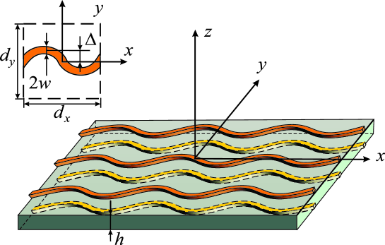
Fig. 1:

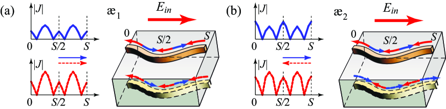
Fig. 2:

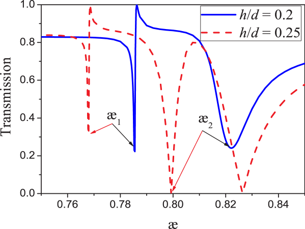
Fig. 3:

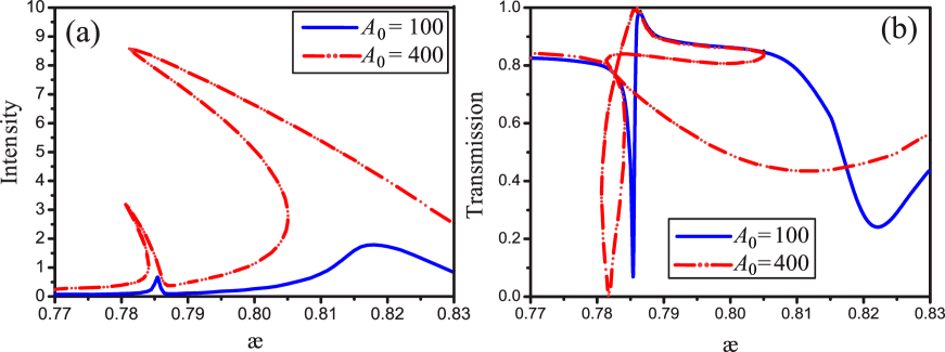
Fig. 4:

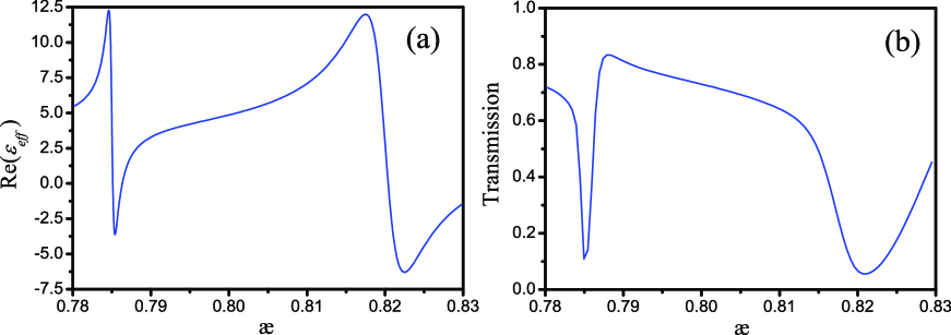
Fig. 5:

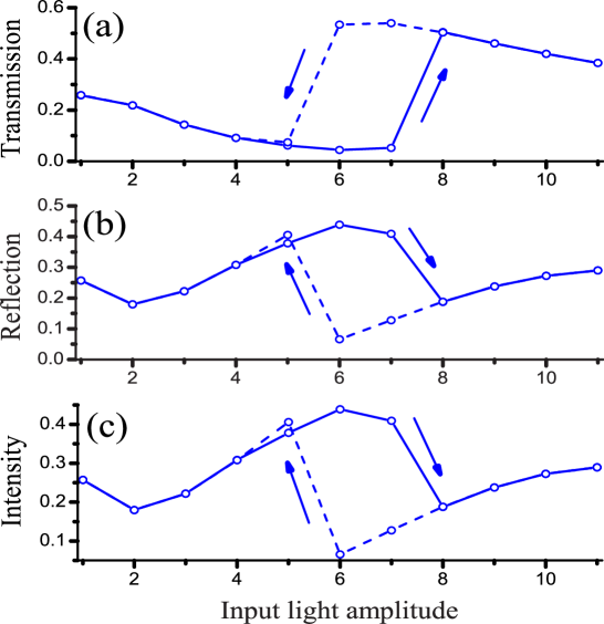
Fig. 6:

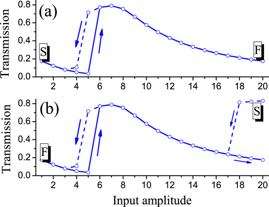
Fig. 7:

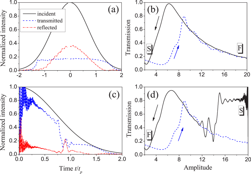
Fig. 8:

References

- [1] Y. S. Kivshar, “Nonlinear optics: The next decade,” Opt. Express, Vol. 16, 22126, 2008, http://www.opticsexpress.org/abstract.cfm?URI=oe-16-26-22126.
- [2] B. Wang, J. Zhou, T. Koschny, and C. M. Soukoulis, “Nonlinear properties of split-ring resonators,” Opt. Express, Vol. 16, 16058, 2008, http://dx.doi.org/10.1364/OE.16.016058.
- [3] I. V. Shadrivov, A. B. Kozyrev, D. W. van der Weide, and Y. S. Kivshar, “Tunable transmission and harmonic generation in nonlinear metamaterials,” Appl. Phys. Lett., Vol. 93, 161903, 2008, http://link.aip.org/link/doi/10.1063/1.2999634.
- [4] E. Poutrina, D. Huang, and D. R. Smith, “Analysis of nonlinear electromagnetic metamaterials,” New J. Phys., Vol. 12, 093010, 2010, http://dx.doi.org/10.1088/1367-2630/12/9/093010.
- [5] N. Papasimakis, Y. H. Fu, V. A. Fedotov, S. L. Prosvirnin, D. P. Tsai, and N. I. Zheludev, “Metamaterial with polarization and direction insensitive resonant transmission response mimicking electromagnetically induced transparency,” Appl. Phys. Lett., Vol. 94, 211902, 2009, http://dx.doi.org/10.1063/1.3138868.
- [6] M. Kitano, Y. Tamayama, and T. Nakanishi, “Coupled-resonator-based metamaterials,” IEICE Electronics Express, Vol. 9, 512012, http://www.jstage.jst.go.jp/article/elex/9/2/9_2_51/_article.
- [7] S. Prosvirnin and S. Zouhdi, “Resonances of closed modes in thin arrays of complex particles,” in Advances in Electromagnetics of Complex Media and Metamaterials, edited by S. Zouhdi and M. Arsalane Kluwer Academic Publishers, the Netherlands, 2003, 281–290.
- [8] V. A. Fedotov, M. Rose, S. L. Prosvirnin, N. Papasimakis, and N. I. Zheludev, “Sharp trapped-mode resonances in planar metamaterials with a broken structural symmetry,” Phys. Rev. Lett., Vol. 99, 147401, 2007, http://link.aps.org/doi/10.1103/PhysRevLett.99.147401.
- [9] V. V. Khardikov, E. O. Iarko, and S. L. Prosvirnin, “Trapping of light by metal arrays,” J. Opt., Vol. 12, 045102, 2010, http://dx.doi.org/10.1088/2040-8978/12/4/045102.
- [10] Z. L. Sámson, K. F. MacDonald, F. D. Angelis, B. Gholipour, K. Knight, C. C. Huang, E. D. Fabrizio, D. W. Hewak, and N. I. Zheludev, “Metamaterial electro-optic switch of nanoscale thickness,” Appl. Phys. Lett., Vol. 96, 143105, 2010, http://link.aip.org/link/doi/10.1063/1.3355544.
- [11] V. R. Tuz, S. L. Prosvirnin, L. A. Kochetova, “Optical bistability involving planar metamaterials with broken structural symmetry,” Phys. Rev. B, Vol. 82, 233402, 2010, http://link.aps.org/doi/10.1103/PhysRevB.82.233402.
- [12] V. R. Tuz and S. L. Prosvirnin, “All-optical switching in planar metamaterial with high structural symmetry,” Eur. Phys. J. Appl. Phys., Vol. 56, 30401 2011, http://www.epjap.org/10.1051/epjap/2011110145.
- [13] V. R. Tuz, V. S. Butylkin, and S. L. Prosvirnin, “Enhancement of absorption bistability by trapping-light planar metamaterial,” J. Opt., Vol. 14, 045102, 2012, http://iopscience.iop.org/2040-8986/14/4/045102/.
- [14] V.Dmitriev, V. Tuz, S. Prosvirnin, and M. N. Kawakatsu, “Electromagnetic controllable surfaces based on trapped-mode effect,” Adv. Electromagn., Vol. 1, 89, 2012, http://aemjournal.org/index.php/AEM/article/view/109.
- [15] V. A. Fedotov, P. L. Mladyonov, S. L. Prosvirnin, and N. I. Zheludev, “Planar electromagnetic metamaterial with a fish scale structure,” Phys. Rev. E, Vol. 72, 056613, 2005, http://link.aps.org/doi/10.1103/PhysRevE.72.056613.
- [16] X. Zhang, J. Gu, W. Cao, J. Han, A. Lakhtakia, and W. Zhang, “Bilayer-fish-scale ultrabroad terahertz bandpass filter,” Opt. Lett., Vol. 37, 906, 2012, http://dx.doi.org/10.1364/OL.37.000906.
- [17] H. J. Rance, T. J. Constant, A. P. Hibbins, and J. R. Sambles, “Surface waves at microwave frequencies excited on a zigzag metasurface,” Phys. Rev. B, Vol. 86, 125144, 2012, http://link.aps.org/doi/10.1103/PhysRevB.86.125144.
- [18] S. L. Prosvirnin, S. A. Tretyakov, and P. L. Mladyonov, “Electromagnetic wave diffraction by planar periodic gratings of wavy metal strips,” J. Electromagn. Waves Appl., Vol. 16, 421, 2002, http://dx.doi.org/10.1163/156939302X01263.
- [19] P. L. Mladyonov and S. L. Prosvirnin, “Wave diffraction by double-periodic gratings of continuous curvilinear metal strips placed on both sides of a dielectric layer,” Radio Physics and Radio Astronomy, Vol. 1, 309, 2010, http://dx.doi.org/10.1615/RadioPhysicsRadioAstronomy.v1.i4.50.
- [20] M. N. Kawakatsu, V. A. Dmitriev, and S. L. Prosvirnin, “Microwave frequency selective surfaces with high Q-factor resonance and polarization insensitivity,” J. Electromagn. Waves Appl., Vol. 24, 261, 2010, http://dx.doi.org/10.1163/156939310790735741.
- [21] P. Mladenov, S. Prosvirnin, S. Tretyakov, S. Zouhdi, “Planar arrays of wavy microstrip lines as thin resonant magnetic walls”, Antennas and Propagation Society International Symposium, IEEE, 2003, Vol. 2, 1103–1106, http://dx.doi.org/10.1109/APS.2003.1219428.
- [22] D. Sievenpiper, L. Zhang, R. F. J. Broas, N. Alexopolous, and E. Yablonovitch, “High-impedance electromagnetic surfaces with a forbidden frequency band,” Microwave Theory and Techniques, IEEE Transactions on, Vol. 47, 2059, 1999, http://dx.doi.org/10.1109/22.798001.
- [23] E. D. Palik, Handbook of Optical Constants of Solids, Academic Press, Boston, 1991.
- [24] V. V. Yatsenko, S. I. Maslovski, S. A. Tretyakov, S. L. Prosvirnin, and S. Zouhdi, “Plane-wave reflection from double arrays of small magnetoelectric scatterers,” Antennas and Propagation, IEEE Transactions on, Vol. 51, 2, 2003, http://dx.doi.org/10.1109/TAP.2003.808569.
- [25] H. M. Gibbs, Optical bistability: controlling light with light, Academic Press, Orlando, 1985.
- [26] A. E. Miroshnichenko, S. Flach, and Yu. S. Kivshar, “Fano resonances in nanoscale structures”, Rev. Mod. Phys., Vol. 82, 2257, 2010, http://link.aps.org/doi/10.1103/RevModPhys.82.2257.
- [27] A. V. Novitsky, V. M. Galynsky, S. V. Zhukovsky, “Asymmetric transmission in planar chiral split-ring metamaterials: Microscopic Lorentz-theory approach,” Phys. Rev. B, Vol. 86, 075138, 2012, http://link.aps.org/doi/10.1103/PhysRevB.86.075138.
- [28] A. F. Oskooi, D. Roundy, M. Ibanescu, P. Bermel, J. D. Joannopoulos, and S. G. Johnson, “MEEP: A flexible free-software package for electromagnetic simulations by the FDTD method,” Computer Physics Communications, Vol. 181, 687, 2010, http://dx.doi.org/doi:10.1016/j.cpc.2009.11.008.
- [29] S. C. H. A. Taflove, Computational electrodynamics: the Finite-Difference Time-Domain method, Artech House, Boston, 2000.
- [30] A. A. Zharov, R. E. Noskov, and M. V. Tsarev, “Plasmon-induced terahertz radiation generation due to symmetry breaking in a nonlinear metallic nanodimer,” J. Appl. Phys., Vol. 106, 073104, 2009, http://scitation.aip.org/content/aip/journal/jap/106/7/10.1063/1.3225606.
- [31] N. Lapshina, R. Noskov, and Yu. Kivshar, “Nanoradar based on nonlinear dimer nanoantenna,” Opt. Lett., Vol. 37, 3921, 2012, http://ol.osa.org/abstract.cfm?URI=ol-37-18-3921.
- [32] N. S. Lapshina, R. E. Noskov, and Yu. S. Kivshar, “Nonlinear nanoantenna with self-tunable scattering pattern,” JETP Lett., Vol. 96, 759, 2013, http://dx.doi.org/10.1134/S0021364012240071.