Unsupervised Ranking of Multi-Attribute Objects Based on Principal Curves

Abstract

Unsupervised ranking faces one critical challenge in evaluation applications, that is, no ground truth is available. When PageRank and its variants show a good solution in related subjects, they are applicable only for ranking from link-structure data. In this work, we focus on unsupervised ranking from multi-attribute data which is also common in evaluation tasks. To overcome the challenge, we propose five essential meta-rules for the design and assessment of unsupervised ranking approaches: scale and translation invariance, strict monotonicity, linear/nonlinear capacities, smoothness, and explicitness of parameter size. These meta-rules are regarded as high level knowledge for unsupervised ranking tasks. Inspired by the works in [8] and [14], we propose a ranking principal curve (RPC) model, which learns a one-dimensional manifold function to perform unsupervised ranking tasks on multi-attribute observations. Furthermore, the RPC is modeled to be a cubic Bézier curve with control points restricted in the interior of a hypercube, thereby complying with all the five meta-rules to infer a reasonable ranking list. With control points as the model parameters, one is able to understand the learned manifold and to interpret the ranking list semantically. Numerical experiments of the presented RPC model are conducted on two open datasets of different ranking applications. In comparison with the state-of-the-art approaches, the new model is able to show more reasonable ranking lists.

1 Introduction

Figure 1: Hierarchical diagram of ranking approaches. RPC is an unsupervised ranking approach based on multi-attribute observations for objects.

From the viewpoint of machine learning, ranking can be performed in an either supervised or unsupervised way as shown in the hierarchical structure in Fig. 1. When supervised ranking [1] is able to evaluate the ranking performance from the given ground truth, unsupervised ranking seems more challenging because no ground truth label is available. Modelers or users will encounter a more difficult issue below:

“How can we insure that the ranking list from the unsupervised ranking is reasonable or proper?”

From the viewpoint of given data types, ranking approaches can be further divided into two categories: ranking based on link structure and ranking based on multi-attribute data. PageRank [2] is one of the representative unsupervised approaches to rank items which have a linking network (e.g. websites). But PageRank and its variants do not work for ranking candidates which have no links. In this paper, we focus on unsupervised ranking approaches on a set of objects with multi-attribute numerical observations.

To rank from multi-attribute objects, weighted summation of attributes is widely used to provide a scalar score for each object. But different weight assignments give different ranking lists such that ranking results are not convincing enough. The first principal component analysis (PCA) provides a weight learning approach [5], by which the score for each object is determined by its principal component on the skeleton of the data distribution. However, it encounters problems when the data distribution is nonlinearly shaped. Although kernel PCA [5] is proposed to attack this problem, the mapping to the kernel space is not order-preserving, which is the basic requirement for a ranking function. Neither dimension reduction methods [6] nor vector quantization [9] can assign scores for multi-attribute observations.

As the nonlinear extension of the first PCA, principal curves can be used to perform a ranking task [10, 8]. A principal curve provides an ordering of data points by the ordering of threading through their projected points on the curve (illustrated by Fig. 2) which can be regarded as the “ranking skeleton”. However, not all of principal curve models are capable of performing a ranking task. Polyline approximation of a principal curve [11] fails to provide a consistent ranking rule due to non-smoothness at connecting points. Besides, it fails to guarantee order-preserving. Order-preserving can not be guaranteed either by a general principal curve model (e.g. [19]) which is not modeled specially for ranking tasks. The problem can be tackled by the constraint of strict monotonicity which is one of the constraints we present for ranking functions in this paper. Example 1 shows that strict monotonicity is a necessary condition for a ranking function but was neglected by all other investigations.

Example 1.

Suppose we want to evaluate life qualities of countries with a principal curve based on two attributes: LEB and GDP. Each country is a data point in the two-dimensional plane of LEB and GDP. If the principal curve is approximated by a polyline as in Fig. 2(a), the piece of the horizontal line is not strictly monotone. It makes the same ranking solution for $\mathbf{x}_{1}=(58,1.4)$ and $\mathbf{x}_{2}=(58,16.2)$ but $\mathbf{x}_{2}$ should be ranked higher than $\mathbf{x}_{1}$. For a general principal curve like the curve in Fig. 2(b) which is not monotone, two pairs of points are ordered unreasonably. The pair, $\mathbf{x}_{3}=(74,40.2)$ and $\mathbf{x}_{4}=(82,40.2)$, are put in the same place of the ranking list since they are projected to the same point which has the vertical tangent line to the curve. But $\mathbf{x}_{4}$ should be ranked higher for its higher LEB than $\mathbf{x}_{3}$. Another pair, $\mathbf{x}_{5}=(75,62.5)$ and $\mathbf{x}_{6}=(81,64.8)$, are also put in the same place but apparently $\mathbf{x}_{6}$ should be ranked higher than $\mathbf{x}_{5}$. With strict monotonicity, these points would be in the order that they are.

      

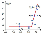
(a) Polyline Approximation (non-strict monotonicity)

(b) A General Principal Curve (non-monotonicity)

Figure 2: Examples on a monotonicity property for ranking with principal curves.

Following the principle of “let the data speak for themselves” [12], this work tries to attack problems for unsupervised ranking of multi-attribute objects with principal curves . First, ranking performance is taken into account for the design of ranking functions. It is known that knowledge of a given task can always improve learning performance [13]. The reason why PageRank produces a commonly acceptable search result for a query, lies on that PageRank algorithm is designed by integrating the knowledge about backlinks [2]. For multi-attribute objects with no linking networks, knowledge about ranking functions can be taken into account to make ranking functions produce reasonable ranking lists. In this work, we present five essential meta-rules for ranking rules (Fig. 3). These meta-rules can be capable of assessing the reasonability of ranking lists for unsupervised ranking.

Second, principal curves should be modeled to be able to serve as ranking functions. As referred in [8], ranking with a principal curve is performed on the learned skeleton of data distribution. But not all principal curve models are capable of producing reasonable ranked lists when no ranking knowledge is embedded into principal curve models. Motivated by [14], the principal curve can be parametrically designed with a cubic Bézier curve. We will show in Section 4 that the parameterized principal curve has all the five meta-rules with constraints on control points and that its existence and convergency of learning algorithm are proved theoretically. Therefore, the parameterized principal curve is capable of making a reasonable ranking list.

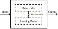
Figure 3: Motivation of RPC model for unsupervised ranking.

The following points highlight the main contributions of this paper:

• We propose five meta-rules for unsupervised ranking, which serve as high-level guidance in the design and assessment of unsupervised ranking approaches for multi-attribute objects. We justify that the five meta-rules are essential in applications, but unfortunately some or all of them were overlooked by most of ranking approaches.

• A ranking principal curve (RPC) model is presented for unsupervised ranking from multi-attribute numerical observations of objects, different from PageRank which ranks from link structure [2]. The presented model can satisfy all of five meta-rules for ranking tasks, while other existing approaches [8] overlooked them.

• We develop the RPC learning algorithm, and theoretically prove the existence of a RPC and convergency of learning algorithm for given multi-attribute objects for ranking. With RPC learning algorithm, reasonable ranking lists for openly accessible data illustrate the good performance of the proposed unsupervised ranking approaches.

1.1 Related Works

Domain knowledge can be integrated into leaning models to improve learning performance. By coupling domain knowledge as prior information with network constructions, Hu et al. [13] and Daniels et al. [15] improve the prediction accuracy of neural networks. Recently, monotonicity is taken into consideration as constraints by Kotłowski et al. [16] to improved the ordinal classification performance. For unsupervised ranking, the domain knowledge of monotonicity can also be taken into account and is capable of assessing the ranking performance, other than evaluation of side-effects [17].

Ranking on manifolds has provided a new ranking framework [3, 8, 4, 18], which is different from general ranking functions such as ranking aggregation [7]. As one-dimensional manifolds, principal curves are able to perform unsupervised ranking tasks from multi-attribute numerical observations of objects [8]. But not all principal curve models can serve as ranking functions. For example, Elmap can well portray the contour of a molecular surface [19] but would bring about a biased ranking list due to no guarantee of order-preserving [8]. What’s more, Elmap is hardly interpretable since the parameter size of principal curves is unknown explicitly.

A Bézier curve is a parametrical one-dimensional curve which is widely used in fitting [20]. Hu et al. [14] proved that in two-dimensional space a cubic Bézier curve is strictly monotone with end points in the opposite corner and control points in the interior of the square box as shown in Fig. 4. To avoid confusion, end points refer to the points on both ends of the control polyline (also the end points of the curve) and control points refer to the other vertices of the control polyline in this paper.

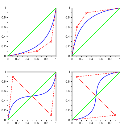
Figure 4: For an increasing monotone function, there are four basic nonlinear shapes [14] of cubic Bézier curves (in blue) which mimic shapes of the control polylines (in red). Curve shapes are determined by the locations of control points.

1.2 Paper Organization

The rest of this paper is organized as follows. Backgrounds of this paper are formalized in the next section. In Section 3, five meta-rules are elaborated for ranking functions. In Section 4, a ranking model, namely ranking principal curve (RPC) model, is defined and formulated with a cubic Bèzier curve which is proved to follow all the five meta-rules for ranking functions. RPC learning algorithm is designed to learn the control points of the cubic Bèzier curve in Section 5. To illustrate the effective performance of the proposed RPC model, applications on real world datasets are carried out in Section 6, prior to summary of this paper in Section 7.

2 Backgrounds

Consider ranking a set of $n$ objects $\mathscr{A}=\{a_{1},a_{2},\cdots,a_{n}\}$ according to $d$ real-valued attributes (or indicators, features) $\mathbf{V}=\{v_{1},v_{2},\cdots,v_{d}\}$. Numerical observations of one object $a\in\mathscr{A}$ on all the attributes comprise an item which is denoted as a vector $\mathbf{x}$ in $d$-dimensional space $\mathbf{R}^{d}$. Ranking objects in $\mathscr{A}$ is equivalent to ranking data points $\mathbf{X}=\{\mathbf{x}_{1},\mathbf{x}_{2},\cdots,\mathbf{x}_{n}\}$. That is, to give the ordering of $a_{i_{1}}\preceq{a_{i_{2}}}\preceq\cdots\preceq{a_{i_{n}}}$ can be achieved by discovering the ordering of $\mathbf{x}_{i_{1}}\preceq{\mathbf{x}_{i_{2}}}\preceq\cdots\preceq{\mathbf{x}_{i_{n}}}$ where $\{i_{1},i_{2},\cdots,i_{n}\}$ is a permutation of $\{1,2,\cdots,n\}$ and $\mathbf{x}_{i}\preceq{\mathbf{x}_{j}}$ means that $\mathbf{x}_{i}$ precedes $\mathbf{x}_{j}$. As there is no label to help with ranking, it is an unsupervised ranking problem from multi-attribute data.

Mathematically, ranking task is to provide a list of totally ordered points. A total order is a special partial order which requires comparability in addition to the requirements of reflexivity, antisymmetry and transitivity for the partial order [21]. Let $\mathbf{x}$ and $\mathbf{y}$ are one pair of points in $\mathbf{X}$. For ranking, if $\mathbf{x}$ and $\mathbf{y}$ are different, they have the ordinal relation of either $\mathbf{x}\preceq\mathbf{y}$ or $\mathbf{y}\preceq\mathbf{x}$. If $\mathbf{x}\preceq\mathbf{y}$ and $\mathbf{y}\preceq\mathbf{x}$, then $\mathbf{y}=\mathbf{x}$ which infers that $\mathbf{x}$ and $\mathbf{y}$ are the same thing.

Remembering that a partial order is associated with a proper cone and that $\mathbf{R}^{d}_{+}$ is a self-dual proper cone [21] $\mathbf{R}^{d}_{+}=\{{\bm{\rho}}:{\bm{\rho}}^{T}\mathbf{x}\geq 0,\forall\mathbf{x}\in\mathbf{R}^{d}_{+}\}$, the order for ranking tasks on $\mathbf{R}^{d}$ is defined in this paper to be

$$\mathbf{x}\preceq\mathbf{y}\Longleftrightarrow\left(\begin{array}[]{c}\delta_{1}(y_{1}-x_{1})\\ \delta_{2}(y_{2}-x_{2})\\ \vdots\\ \delta_{d}(y_{d}-x_{d})\end{array}\right)\in\mathbf{R}^{d}_{+}$$ (1)

where $\mathbf{x}=(x_{1},x_{2},\cdots,x_{d})^{T}$, $\mathbf{y}=(y_{1},y_{2},\cdots,y_{d})^{T}$, and

$$\delta_{j}=\left\{\begin{array}[]{rl}1,&j\in\mathbf{E}\\ -1,&j\in\mathbf{F}\end{array}\right..$$ (2)

It is easy to verify that the order defined by Eq.(1) is a total order with properties of comparability, reflexivity, antisymmetry and transitivity. In Eq.(2), $\mathbf{E}$ and $\mathbf{F}$ are two subsets of $\{1,2,\cdots,d\}$ such that $\mathbf{E}\bigcup\mathbf{F}=\{1,2,\cdots,d\}$ and $\mathbf{E}\bigcap\mathbf{F}=\varnothing$. If let

$$\mathbf{\bm{\alpha}}=(\delta_{1},\delta_{2},\cdots,\delta_{d})^{T}.$$ (3)

$\mathbf{\bm{\alpha}}$ is unique for one given ranking task and varies from task to task. For a given ranking task with defined $\mathbf{\bm{\alpha}}$, $\mathbf{x}$ precedes $\mathbf{y}$ for $x_{j}<y_{j}(j\in\mathbf{E})$ and $x_{j}>y_{j}(j\in\mathbf{F})$.

As $\mathbf{R}$ is totally ordered, we prefer to grade each point with a real value to help with ranking. Assume $\varphi:\mathbf{R}^{d}\mapsto\mathbf{R}$ is the ranking function to assign $\mathbf{x}$ a score which provides the ordering of $\mathbf{x}$. $\varphi$ is required to be order-preserving so that $\varphi(\mathbf{x})$ has the same ordering in $\mathbf{R}$ as $\mathbf{x}$ in $\mathbf{R}^{d}$. In order theory, an order-preserving function is also called isotone or monotone [22].

Definition 1 ([22]).

A function $\varphi:\mathbf{R}^{d}\mapsto\mathbf{R}$ is called monotone (or, alternatively, order-preserving) if

$$\mathbf{x}\preceq\mathbf{y}\Longrightarrow\varphi(\mathbf{x})\leq\varphi(\mathbf{y})$$ (4)

and strictly monotone if

$$\mathbf{x}\preceq\mathbf{y},\mathbf{x}\neq\mathbf{y}\Longrightarrow\varphi(\mathbf{x})<\varphi(\mathbf{y})$$ (5)

Order-preserving is the basic requirement for a ranking function. For a partially ordered set, $\varphi$ should assign a score to $\mathbf{x}$ no more than the score to $\mathbf{y}$ if $\mathbf{x}\preceq\mathbf{y}$. Moreover, if $\mathbf{x}\neq\mathbf{y}$ also holds, the score assigned to $\mathbf{x}$ must be smaller than the score to $\mathbf{y}$. As $\mathscr{A}$ is totally ordered and different points should be assigned with different scores, the ranking function is required to be strictly monotone as stated by Eq.(5). Otherwise, the ranking rule would be meaningless due to breaking the ordering in original data space $\mathbf{R}^{d}$.

Example 2.

In addition to the two indicators in Example 1, another two indicators are taken to evaluate life qualities of countries: IMR and Tuberculosis. It is easily known that the life quality of one country would be higher if it has a higher LEB and GDP while a lower IMR and Tuberculosis. Let numerical observations on four countries to be $\mathbf{x}_{I}=(2.1,62.7,75,59)$, $\mathbf{x}_{M}=(11.3,75.5,12,30)$, $\mathbf{x}_{G}=(32.1,79.2,6,4)$, and $\mathbf{x}_{N}=(47.6,80.1,3,3)$ respectively. By Eq.(1), they have the ordering $\mathbf{x}_{I}\preceq\mathbf{x}_{M}\preceq\mathbf{x}_{G}\preceq\mathbf{x}_{N}$ with ${\bm{\alpha}}=(1,1,-1,-1)^{T}$. In this case, $\mathbf{E}=\{1,2\}$ and $\mathbf{F}=\{3,4\}$. Let $\varphi(\mathbf{x}_{I})=0.407$, $\varphi(\mathbf{x}_{M})=0.593$, $\varphi(\mathbf{x}_{G})=0.785$ and $\varphi(\mathbf{x}_{N})=0.891$. Then $\varphi$ is a strictly monotone mapping which strictly preserves the ordering in $\mathbf{R}^{4}$.

Recall that a differentiable function $f:\mathbf{R}\mapsto\mathbf{R}$ is nondecreasing if and only if $f^{\prime}(x)\geq 0$ for all $x\in\mathbf{dom}f$, and increasing if $f^{\prime}(x)>0$ for all $x\in\mathbf{dom}f$ (but the converse is not true) [23]. They are readily extended to the case of monotonicity in Definition 1 with respect to the order defined by Eq.(1).

Theorem 1 ([21]).

Let $\varphi:\mathbf{R}^{d}\mapsto\mathbf{R}$ be differentiable. $\varphi$ is monotone if and only if

$$\nabla\varphi(\mathbf{x})\succeq\mathbf{0}$$ (6)

where $\mathbf{0}$ is the zero vector. $\varphi$ is strictly monotone if

$$\nabla\varphi(\mathbf{x})\succ\mathbf{0}$$ (7)

Theorem 1 provides first-order conditions for monotonicity. Note that ‘$\succ$’ denotes a strict partial order [21]. Let

$$\nabla\varphi(\mathbf{x})=\left(\frac{\partial\varphi}{\partial x_{1}},\frac{\partial\varphi}{\partial x_{2}},\cdots,\frac{\partial\varphi}{\partial x_{d}}\right)^{T}.$$ (8)

$\nabla\varphi(\mathbf{x})\succ\mathbf{0}$ infers $\frac{\partial\varphi}{\partial x_{j}}>0$ for $j\in\mathbf{E}$ and $\frac{\partial\varphi}{\partial x_{j}}<0$ for $j\in\mathbf{F}$. $\nabla\varphi(\mathbf{x})\succ\mathbf{0}$ infers that each component of $\nabla\varphi(\mathbf{x})$ does not equal to zero. By the case of strict monotonicity in Theorem 1, $\nabla\varphi(\mathbf{x})\succ\mathbf{0}$ infers not only that $\varphi$ is strictly monotone from $\mathbf{R}^{d}$ to $\mathbf{R}$, but also that the value $s=\varphi(\mathbf{x})$ is increasing with respect to $x_{j}(j\in\mathbf{E})$ and decreasing with respect to $x_{j}(j\in\mathbf{F})$. Vice versa, if $\frac{\partial\varphi}{\partial x_{j}}$ is bigger than zero for $j\in\mathbf{E}$ and smaller than zero for $j\in\mathbf{F}$, $\nabla\varphi(\mathbf{x})\succ\mathbf{0}$ holds and infers $\varphi$ is a strictly monotone mapping. Lemma 1 can be concluded immediately.

Lemma 1.

$s=\varphi(\mathbf{x})$ is strictly monotone if and only if $s$ is strictly monotone along $x_{i}$ with fixed the others $x_{j}(j\neq i)$.

Further more, a strictly monotone mapping infers a one-to-one mapping that for a value $s\in\mathbf{rang}\varphi$ there is exactly one point $\mathbf{x}\in\mathbf{dom}\varphi$ such that $\varphi(\mathbf{\mathbf{x}})=s$. If the point $\mathbf{x}$ is denoted by $\mathbf{x}=\mathbf{f}(s)$, $\mathbf{f}:\mathbf{R}\mapsto\mathbf{R}^{d}$ is called the inverse mapping of $\varphi$ and inherits the property of strict monotonicity of its origin $\varphi$.

Theorem 2.

Assume $\nabla\varphi(\mathbf{x})\succ\mathbf{0}$. There exists an inverse mapping denoted by $\mathbf{f}:\mathbf{rang}\varphi\mapsto\mathbf{dom}\varphi$ such that $\nabla\mathbf{f}(s)\succ\mathbf{0}$ holds for all $s\in\mathbf{rang}\varphi$, that is for $\forall s_{1},s_{2}\in\mathbf{rang}\varphi$

$$s_{1}<s_{2}\Longrightarrow\mathbf{f}(s_{1})\preceq\mathbf{f}(s_{2}),\mathbf{f}(s_{1})\neq\mathbf{f}(s_{2}).$$ (9)

Proof of Theorem 2 can be found in Appendix B. The theorem also holds in the other direction. Assuming $\mathbf{f}:\mathbf{R}\mapsto\mathbf{R}^{d}$, if $\nabla\mathbf{f}(s)\succ\mathbf{0}$, there exists an inverse mapping $\varphi:\mathbf{rang}\mathbf{f}\mapsto\mathbf{dom}\mathbf{f}$ and $\nabla\varphi(\mathbf{x})\succ\mathbf{0}$ holds for all $\mathbf{x}\in\mathbf{rang}\mathbf{f}$. Because of the one-to-one correspondence, $\mathbf{f}$ and $\varphi$ share the same geometric properties such as scale and translation invariance, smoothness and strict monotonicity [23].

3 Meta-Rules

As a ranking function for $\varphi:\mathbf{R}^{d}\mapsto\mathbf{R}$, $\varphi(\mathbf{x})$ outputs a real value $s=\varphi(\mathbf{x})$ as the ranking score for a given point $\mathbf{x}$. The ranking list of objects would be provided by sorting their ranking scores in ascending/descending order. Since unsupervised ranking has no label information to verify the ranking list, we restrict ranking functions with five essential features to guarantee that a reasonable ranking list is provided. These features are capable of serving as high-level guidance of modeling ranking functions. They are also capable of serving as high-level assessments for unsupervised ranking performance, different from assessments for supervised ranking performance which take qualities of ranking labels. Any functions from $\mathbf{R}^{d}$ to $\mathbf{R}$ with all the five features can serve as ranking functions and be able to provide a reasonable ranking list. These features are rules for ranking rules, namely meta-rules.

3.1 Scale and Translation Invariance

Definition 2 ([24]).

A ranking rule is invariant to scale and translation if for $\mathbf{x}\preceq\mathbf{y}$

$$\varphi(\mathbf{x})\leq\varphi(\mathbf{y})\Longleftrightarrow\varphi(\mathbf{L}(\mathbf{x}))\leq\varphi(\mathbf{L}(\mathbf{y})).$$ (10)

where $\mathbf{L}(\cdot)$ performs scale and translation.

Numerical observations on different indicators are taken on different dimensions of quantity. In Example 1, GDP is measured in thousands of dollars while LEB ranges from 40 to 90 years. They are not in the same dimensions of quantity. As a general data preprocessing technique, scale and translation can take them into the same dimensions (e.g. $[0,1]$) while preserving their original ordering. If let $\mathbf{L}$ be a linear transformation on $\mathbf{R}^{d}$, we have $\mathbf{x}\preceq\mathbf{y}\Longleftrightarrow\mathbf{L}(\mathbf{x})\preceq\mathbf{L}(\mathbf{y})$ for $\mathbf{x},\mathbf{y}\in\mathbf{R}^{d}$ [24]. Therefore, a ranking function $\varphi(\mathbf{x})$ should produce the same ranking list before and after scaling and translating.

3.2 Strict Monotonicity

Definition 3 ([22]).

$\varphi(\mathbf{x})$ is strictly monotone if $\varphi(\mathbf{x}_{i})<\varphi(\mathbf{x}_{j})$ for $\mathbf{x}_{i}\preceq\mathbf{x}_{j}$ and $\mathbf{x}_{i}\neq\mathbf{x}_{j}(i\neq{j})$ .

Strict monotonicity in Definition 1 is specified here as one of meta-rules for ranking. For ordinal classification problem, monotonicity is a general constraint since two different objects would be classified into the same class [16]. But for the ranking problem discussed in this paper, it requires the strict monotonicity since different objects should have different scores for ranking. $\varphi(\mathbf{x}_{i})=\varphi(\mathbf{x}_{j})$ holds if and only if $\mathbf{x}_{i}=\mathbf{x}_{j}(i\neq{j})$. In Example 1, $\mathbf{x}_{1}\preceq\mathbf{x}_{2}$ and $\mathbf{x}_{i}\neq\mathbf{x}_{j}$ indicate that a higher score should be assigned to $\mathbf{x}_{2}$ than $\mathbf{x}_{1}$. And so do $\mathbf{x}_{3}$ and $\mathbf{x}_{4}$. Therefore, the ranking function $\varphi(\mathbf{x})$ is required to be a strictly monotone mapping. Otherwise, the ranking list would be not convincing. $\varphi$ in Example 2 is to the point referred here.

3.3 Linear/Nonlinear Capacities

Definition 4.

$\varphi(\mathbf{x})$ has the capacities of linearity and nonlinearity if $\varphi(\mathbf{x})$ is able to depict the relationship of both linearity and nonlinearity.

Taking the ranking task in Example 1 for illustration, one has no knowledge about the relationship between LEB and the score. The score might be a either linear or nonlinear function of LEB. It is the similar case for the relationship between GDP and the score. Therefore, $t=\varphi(\mathbf{x})$ should embody both of the linear and nonlinear relationships between $t$ and $x_{j}$. For the ranking task in Example 1, the ranking function $\varphi$ should be a linear function of LEB for fixed GDP if LEB is linear with $t$. Meanwhile, $\varphi$ should also be a nonlinear function of GDP for fixed LEB if GDP is nonlinear with $t$.

3.4 Smoothness

Definition 5 ([23]).

$\varphi(\mathbf{x})$ is smooth if $\varphi(\mathbf{x})$ is $\mathscr{C}^{h}(h\geq 1)$.

In mathematical analysis, a function is called smooth if it has derivatives of all orders [23]. Yet a ranking function $\varphi(\mathbf{x})$ is required to be of class $\mathscr{C}^{h}$ where $h\geq 1$. That is, $\varphi(\mathbf{x})$ is continuous and has the first-order derivative $\nabla\varphi(\mathbf{x})$. The first-order derivative $\nabla\varphi(\mathbf{x})$ guarantees that $\varphi(\mathbf{x})$ will exert a consistent ranking rule for all objects and the ranking rule would be not abruptly changed for some object. Taking the polyline in Fig. 2 for illustration, it is of class $\mathscr{C}^{0}$ but not of class $\mathscr{C}^{1}$ because it is continuous but not differentiable at the connecting vertex of the two lines. This would lead to an unreasonable ranking for those points projected to the vertex.

3.5 Explicitness of Parameter Size

Definition 6.

$\varphi(\mathbf{x})$ has the property of explicitness if $\varphi(\mathbf{x})$ has known parameter size for a fair comparison among ranking models.

Hu et al. [13] considered that nonparametric approaches are a class of “black-box” approaches since they can not be interpreted by our intuition. As a ranking function, $\varphi(\mathbf{x})$ should be semantically interpretable so that $\varphi(\mathbf{x})$ has systematical meanings. For example, $\varphi(\mathbf{x})={\bm{\theta}}^{T}\mathbf{x}$ gives explicitly the linear expression with parameter size $d$ which is the dimension of the parameter $\bm{\theta}$. It can be interpreted that the score of $\mathbf{x}$ is linear with $\mathbf{x}$ and the parameter $\bm{\theta}$ is the allocation proportion vector of indicators for ranking. Moreover, if there is another ranking model with the same characteristics, $\varphi(\mathbf{x},{\bm{\theta}})$ would be more applicable if it has a smaller size of parameters.

These five meta-rules above is the guidance of designing a reasonable and practical ranking function. To perform a ranking task, a ranking function should satisfy all the five meta-rules above to produce a convincing ranking list. Any ranking function that breaks any of them would produce a biased and unreasonable ranking list. In this sense, they can be regarded as high-level assessments for unsupervised ranking performance.

4 Ranking Principal Curves

In this section, we propose a ranking principal curve (RPC) model to perform an unsupervised ranking task with a principal curve which has all the five meta-rules. The RPC is parametrically designed to a cubic Bézier curve with control points restricted in the interior of a hypercube.

4.1 RPC Model

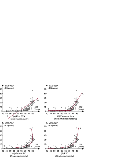
Figure 5: Schematic plots of ranking skeletons (heavy solid lines or curves in red). Circle points: observations of countries on two indicators: LEB and GDP.

The simplest ranking rule is the first PCA which summarizes the data in $d$-dimensional space with the largest principal component line [25]. The first PCA seeks the direction $\mathbf{w}$ that explains the maximal variance of the data cloud. Then $\mathbf{x}$ is orthogonally projected by $\mathbf{w}^{T}\mathbf{x}$ onto the line passing through the mean ${\bm{\mu}}$. The line can be regarded as the ranking skeleton. Projected points take an ordering along the ranking skeleton which is just the ordering of their first principal components computed by $\mathbf{w}^{T}\mathbf{x}$. Let $s=\mathbf{w}^{T}\mathbf{x}$ and an ordering of $s$ gives the ordering of $\mathbf{x}$. As a ranking function, the first PCA is smooth, explicitly expressed, and invariant to scale and translation. It works well for the skeleton of slender ellipse distributing data. However, the first PCA can hardly depict the skeleton of data distributions like crescents (Fig. 5(a)) such that the produced ranking list is not convincing. What’s more, the first PCA might be non-strictly monotone when the direction $\mathbf{w}$ is parallel to one coordinate axis such that it can not discriminate those points like $\mathbf{x}_{1}$ and $\mathbf{x}_{2}$ in Example 1 since they will be projected to the same points if the first PCA is on the direction parallel to the horizontal line. The problems referred above hinder the first PCA from extensive applications in comprehensive evaluation.

Recalling that principal curves are nonlinear extensions of the first PCA [10], we try to summarize multiple indicators in the data space with a principal curve (Appendix A gives a brief review of principal curves). Assuming $\mathbf{f}(s,{\bm{\theta}})(\bm{\theta}\in\mathbf{\Theta})$ is the principal curve of a given data cloud, it provides an ordering of projected points on the principal curve, in a way similar to the first PCA. Intuitively, the principal curve is a good choice to perform ranking tasks. On the one hand, unsupervised ranking could only rely on those numerical observations for ranking candidates on given attributes. For the dataset with a linking network, PageRank can calculate a score with backlinks for each point [2]. When there is no link between points, a score can still be calculated according to the ranking skeleton, instead of link structure. On the other hand, the principal curve reconstructs $\mathbf{x}$ according to $\mathbf{x}=\mathbf{f}(s,{\bm{\theta}})+{\bm{\varepsilon}}$, instead of $\mathbf{x}=\mathbf{\bm{\mu}}+s\mathbf{w}+{\bm{\varepsilon}}$ for the first PCA. To perform ranking tasks, a ranking function assigns a score $s$ to $\mathbf{x}$ by $s=\varphi(\mathbf{x},{\bm{\theta}})$. Actually, noise is inevitable due to measuring errors and influence from exclusive indicators from $\mathbf{V}$. Thus the latent score should be produce after removing noise from $\mathbf{x}$, that is $s=\varphi(\mathbf{x}-{\bm{\varepsilon}},{\bm{\theta}})$. As a ranking function, $\varphi$ is assumed to be strictly monotone. Thus, data points and scores are one-to-one correspondence and there exists an inverse function $\mathbf{f}$ for $\varphi$ such that

$$\mathbf{x}=\mathbf{f}(s,{\bm{\theta}})+{\bm{\varepsilon}}$$ (11)

which is the very principal curve model[10]. The inverse function can be taken as the generating function for numerical observations from the score $s$ which can be regarded to be pre-existing.

As stated in Section 3, there are five meta-rules for a function $\varphi(\mathbf{x},{\bm{\theta}})$ to serve as a ranking rule. As $\varphi(\mathbf{x},{\bm{\theta}})$ is required to be strictly monotone, there exists an inverse function $\mathbf{f}(s,{\bm{\theta}})$ which is also strictly monotone by Theorem 2. Correspondingly, $\varphi$ and its inverse $\mathbf{f}$ share the other properties of scale and translation invariance, smoothness, capacities of linearity and nonlinearity, and explicitness of parameter size. A principal curve should also follow all the five meta-rules to serve as a ranking function. However, polyline approximations of the principal curve might go against smoothness and strict monotonicity (e.g. Fig. 5(b)). A smooth principal curve would also go against strict monotonicity (e.g. Fig. 5(c)). Both of them would make unreasonable ranking solutions as illustrated in Example 1. Within the framework of Fig. 3, all the five meta-rules can be modeled as constraints to the ranking function. Since a principal curve is defined to be smooth and invariant to scale and translation [10], the constraint of strict monotonicity would make it be capable of performing ranking tasks (e.g. Fig. 5(d)). Naturally, the principal curve should have a known parameter size for interpretability reason. We present Definition 7 for unsupervised ranking with a principal curve.

Definition 7.

A curve $\mathbf{f}(\mathbf{x},{\bm{\theta}})$ in $d$-dimensional space is called a ranking principal curve (RPC) if $\mathbf{f}(\mathbf{x},{\bm{\theta}})$ is a strictly monotone principal curve of given data cloud and it is explicitly expressed with known parameters $\bm{\theta}$ of limited size.

4.2 RPC Formulation with Bézier Curves

To perform a ranking task, a principal curve model should follow all the five meta-rules (Section 3) which can be also similarly defined for $\mathbf{f}$. However, not all of principal curve models can perform ranking tasks. The models in [10, 26, 27, 29] lack of explicitness and can not make a monotone mapping on $\mathbf{R}^{d}$ (Fig. 5(c)). Polyline approximation [11, 28, 19] misses the requirements for smoothness and strictly monotonicity (Fig. 5(b)). A new principal curve model is needed to perform ranking while following all the five meta-rules.

In this paper, an RPC is parametrically modeled with a Bézier curve

$$\mathbf{f}(s)=\sum_{r=0}^{k}B_{r}^{k}(s)\mathbf{p}_{r},s\in[0,1]$$ (12)

which is formulated in terms of Bernstein polynomials [31]

$$B_{r}^{k}(s) = \binom{k}{r}(1-s)^{k-r}s^{r},$$ (13)

$$\binom{k}{r} = \frac{k!}{r!(k-r)!}.$$ (14)

In Eq.(12), $\mathbf{p}_{r}\in{\mathbf{R}^{d}}$ are control and end points of the Bézier curve which are in the place of the function parameters $\bm{\theta}$ in Eq.(11). Particularly, when $k=3$, Eq.(12) has the matrix form of

$$\mathbf{f}(s)=\mathbf{PMz}.$$ (15)

where

$$\mathbf{P} = (\mathbf{p}_{0},\mathbf{p}_{1},\mathbf{p}_{2},\mathbf{p}_{3})$$

$$\mathbf{M} = \left(\begin{array}[]{cccc}1&-3&3&-1\\ 0&3&-6&3\\ 0&0&3&-3\\ 0&0&0&1\end{array}\right),\mathbf{z}=\left(\begin{array}[]{c}1\\ s\\ s^{2}\\ s^{3}\end{array}\right)$$

In case $k>3$, the model would become more complex and bring about overfitting problem. In case $k<3$, the model is too simple to represent all possible monotonic curves. $k=3$ is the most suitable degree to perform the ranking task.

A cubic Bézier curve with constraints on control points can be proved to have all the five meta-rules. First of all, the formulation Eq.(12) is a nonlinear interpolation of control points and end points in terms of Bernstein polynomials [31]. These points are the determinant parameters of total size $d\times 4$. Different locations of these points would produce different shapes of nonlinear curves besides straight lines [14]. Scale and translation to Bézier curves are applied to these points without changing the ranking score which is contained in $\mathbf{z}$

$$\mathbf{\Lambda}\mathbf{f}(s)+{\bm{\beta}}=\mathbf{\Lambda}\mathbf{PMz}+{\bm{\beta}}=(\mathbf{\Lambda}\mathbf{P}+{\bm{\beta}})\mathbf{Mz}$$ (17)

where $\mathbf{\Lambda}$ is a diagonal matrix with scaling factors to dimensions and ${\bm{\beta}}$ is the translation vector. This property allows us to put all data into $[0,1]^{d}$ in order to facilitate ranking. What’s more, the derivative of $\mathbf{f}(s)$ is a lower order Bézier curve

$$\frac{d\mathbf{f}(s)}{ds}=k\sum_{j=0}^{k-1}B_{j}^{k-1}(s)(\mathbf{p}_{j+1}-\mathbf{p}_{j})$$ (18)

which involves the calculation of end points and control points. Its derivatives of all orders exist for all $s\in[0,1]$ and thus Eq.(12) is smooth enough. Last but not the least, it has been proved that a cubic Bézier curve can perform the four basic types of strict monotonicity in two-dimensional space [14]. Let end points after scale and translation are denoted by $\mathbf{p}_{0}=\frac{1}{2}(\mathbf{1}-\mathbf{\bm{\alpha}})$ and $\mathbf{p}_{3}=\frac{1}{2}(\mathbf{1}+\mathbf{\bm{\alpha}})$. Control points $\mathbf{p}_{2}$ and $\mathbf{p}_{3}$ are the determinants for nonlinearity of the cubic Bézier curve (Fig. 4). In two-dimensional space, $\mathbf{f}(s)$ is proved to be increasing along each coordinate if control points are restricted in the interior of the hypercube $[0,1]^{d}$ [14]. Thus, a proposition can be deduced by Lemma 1.

Proposition 1.

$\mathbf{f}(s)$ is strictly monotone for $s\in[0,1]$ with $\mathbf{p}_{0}=\frac{1}{2}(\mathbf{1}-\bm{\alpha})$, $\mathbf{p}_{3}=\frac{1}{2}(\mathbf{1}+\bm{\alpha})$ and $\mathbf{p}_{1},\mathbf{p}_{2}\in(0,1)^{d}$.

What is the most important, there always exists an RPC parameterized by a cubic Bézier curve which is strictly monotone for a group of numerical observations. The existence has failed to be proved in many principal curve models [10, 28, 19].

Theorem 3.

Assume that $\mathbf{x}$ is the numerical observation of a ranking candidate and that $E\|{\mathbf{x}}\|^{2}<\infty$. There exists $\mathbf{P}^{*}\in[0,1]^{d}$ such that $\mathbf{f}^{*}(s)=\mathbf{P}^{*}\mathbf{Mz}$ is strictly monotone and

$$J(\mathbf{P}^{*})=\inf\left\{J(\mathbf{P})=E\left(\inf_{s}\|{\mathbf{x}-\mathbf{PMz}}\|^{2}\right)\right\}.$$ (19)

Proof of Theorem 3 can be found in Appendix C.

5 RPC Learning Algorithm

To perform unsupervised ranking from the numerical observations of ranking candidates $\mathbf{X}=(\mathbf{x}_{1},\mathbf{x}_{2},\cdots,\mathbf{x}_{n})$, we should first learn control points of the curve in Eq.(12). The optimal points achieve the infimum of the estimation of $J(\mathbf{P})$ in Eq.(19). By the principal curve definition proposed by Hastie et al.[10], the RPC is the curve which minimizes the summed residual ${\bm{\varepsilon}}$. Therefore, the ranking task is formulated as a nonlinear optimization problem

$$\min J(\mathbf{P},\mathbf{s})=\sum_{i=1}^{n}\|\mathbf{x}_{i}-\mathbf{PMz}_{i}\|^{2}$$ (20)

$$s.t. \left.\left(\frac{\partial\mathbf{PMz}}{\partial s}\right)^{T}\left(\mathbf{x}_{i}-\mathbf{PMz}\right)\right|_{s=s_{i}}=0,$$

$$\mathbf{s}=(s_{1},s_{2},\cdots,s_{n}),\mathbf{z}=(1,s,s^{2},s^{3})^{T}$$

$$\mathbf{P}\in{[0,1]^{d\times 4}},\quad s_{i}\in[0,1],$$

$$i=1,2,\cdots,n$$

where Eq.(5) determines $s_{i}$ to find the point on the curve which has the minimum residual to reconstruct $\mathbf{x}_{i}$ by $\mathbf{f}(s_{i})$. Obviously, a local minimizer $(\mathbf{P}^{*},\mathbf{s}^{*})$ can be achieved in an alternating minimization way

$$\mathbf{P}^{(t+1)}=\arg\min\sum_{i=1}^{n}\|\mathbf{x}_{i}-\mathbf{PMz}_{i}^{(t)}\|^{2}$$ (22)

$$\left.\left(\frac{\partial\mathbf{P}^{(t+1)}\mathbf{Mz}}{\partial s}\right)^{T}\left(\mathbf{x}_{i}-\mathbf{P}^{(t+1)}\mathbf{Mz}\right)\right|_{s=s_{i}^{(t+1)}}=0$$ (23)

where $t$ means the $t$th iteration.

The optimal solution of Eq.(22) has an explicit expression. Associate $\mathbf{X}$ with $\mathbf{Z}$

$$\mathbf{Z}=\left(\begin{array}[]{cccc}1&1&\cdots&1\\ s_{1}&s_{2}&\cdots&s_{n}\\ s_{1}^{2}&s_{2}^{2}&\cdots&s_{n}^{2}\\ s_{1}^{3}&s_{2}^{3}&\cdots&s_{n}^{3}\end{array}\right)=\left(\mathbf{z}_{1},\mathbf{z}_{2},\cdots,\mathbf{z}_{n}\right)$$ (24)

and Eq.(20) can be rewritten in matrix form

$$J(\mathbf{P},\mathbf{s}) = \|\mathbf{X}-\mathbf{PMZ}\|_{F}$$ (25)

$$= tr(\mathbf{X}^{T}\mathbf{X})-2tr(\mathbf{PMZ}\mathbf{X}^{T})$$

$$+tr(\mathbf{PMZZ}^{T}\mathbf{M}^{T}\mathbf{P}^{T}).$$

Setting the derivative of $J$ with respect to $\mathbf{P}$ to zero

$$\frac{\partial J}{\partial\mathbf{P}}=2\left(\mathbf{P}(\mathbf{MZ})(\mathbf{MZ})^{T}-\mathbf{X}(\mathbf{MZ})^{T}\right)=0$$ (26)

and remembering $A^{+}=A^{T}(AA^{T})^{+}$ [35], we get an explicitly expression for the minimum point of Eq.(20)

$$\mathbf{P}=\mathbf{X}(\mathbf{MZ})^{T}\left((\mathbf{MZ})(\mathbf{MZ})^{T}\right)^{+}=\mathbf{X}(\mathbf{MZ})^{+}$$ (27)

where $(\cdotp)^{+}$ takes pseudo-inverse computation. Based on the $t$th iterative results $\mathbf{Z}^{(t)}$, the optimal solution can be given by substituting $\mathbf{Z}^{(t)}$ into Eq.(27) which is $\mathbf{P}^{(t+1)}=\mathbf{X}(\mathbf{MZ}^{(t)})^{+}$. However, $(\mathbf{MZ}^{(t)})^{+}$ is computationally expensive in numerical experiments and $\mathbf{X}$ is always ill-conditioned which has a high condition number, resulting in that a very small change in $\mathbf{Z}^{(t)}$ would produce a tremendous change in $\mathbf{P}^{(t+1)}$. $\mathbf{Z}^{(t)}$ is not the optimal solution of Eq.(20) but a intermediate result of the iteration, and $\mathbf{P}^{(t+1)}$ would thereby go far away from the optimal solution. To settle out the problem, we employ the Richardson iteration [37] with a preconditioner $\mathbf{D}$ which is a diagonal matrix with the $L_{2}$ norm of columns of $(\mathbf{MZ}^{(t)})(\mathbf{MZ}^{(t)})^{T}$ as its diagonal elements. Then $\mathbf{P}^{(t+1)}$ is updated according to

$$\mathbf{P}^{(t+1)} = \mathbf{P}^{(t)}-\gamma^{(t)}(\mathbf{P}^{(t)}(\mathbf{MZ}^{(t)})(\mathbf{MZ}^{(t)})^{T}$$ (28)

$$-\mathbf{X}(\mathbf{MZ}^{(t)})^{T})\mathbf{D}^{-1}$$

where $\gamma^{(t)}$ is a scalar parameter such that the sequence $\mathbf{P}^{(t)}$ converges. In practice, we set

$$\gamma^{(t)}=\frac{2}{\lambda_{min}^{(t)}+\lambda_{max}^{(t)}}$$ (29)

where $\lambda_{min}^{(t)}$ and $\lambda_{max}^{(t)}$ is the minimum and maximum eigenvalues of $(\mathbf{MZ}^{(t)})(\mathbf{MZ}^{(t)})^{T}$ respectively [38].

After getting $\mathbf{P}^{(t+1)}$, the score vector $\mathbf{s}^{(t+1)}$ can be calculated as the solution to Eq.(23). Eq.(23) is a quintic polynomial equation which rarely has explicitly expressed roots. In [20], $s_{i}$ for $\mathbf{x}_{i}$ was approximated by Gradient and Gauss-Newton methods respectively. Jenkins-Traub method [32] was also considered to find the roots of the polynomial equation directly. As Eq.(5) is designed to find the minimum distance of point $\mathbf{x}_{i}$ from the curve, we adopt Golden Section Search (GSS) [33] to find the local approximate solution to Eq.(23).

Algorithm 1 Algorithm to learn an RPC.

0:     $\mathbf{X}$: data matrix; $\xi$: a small positive value;

0:     $\mathbf{P}^{*}$: control points of the learned Bézier curve $\mathbf{s}^{*}$: the score vector of objects in the set.

1:  Normalize $\mathbf{X}$ into $[0,1]^{d}$;

2:  Initialize $\mathbf{P}^{(0)}$;

3:  while $\vartriangle{J}>\xi$ do

4:     Adopt GSS to find the approximate solution $\mathbf{s}^{(t)}$;

5:     Compute $\mathbf{P}^{(t+1)}$ using a preconditioner;

6:     if $\vartriangle{J}<0$ then

7:        break;

8:     end if

9:  end while

Algorithm 1 summarizes the alternative optimization procedure. Before performing the ranking task, numerical observations of objects should be normalized into $[0,1]^{d}$ by

$$\hat{\mathbf{x}}=\frac{\mathbf{x}-\mathbf{x}_{min}}{\mathbf{x}_{max}-\mathbf{x}_{min}}$$ (30)

where $\hat{\mathbf{x}}$ is the normalized vector of $\mathbf{x}$, $\mathbf{x}_{min}$ the minimum vector and $\mathbf{x}_{max}$ the maximum vector. Grading scores would be unchanged as scaling and translating are only performed on control points and end points (Eq.(17)) without changing the interpolation values. In Step 2, we initialize the end points as $\mathbf{p}_{0}=\frac{1}{2}(\mathbf{1}-\mathbf{\bm{\alpha}})$ and $\mathbf{p}_{3}=\frac{1}{2}(\mathbf{1}+\mathbf{\bm{\alpha}})$, and randomly select samples as control points. During learning procedure, $\mathbf{P}^{(t)}$ is automatically learned making a Bézier curve to be an RPC in numerical experiments. In Step 6, $\vartriangle{J}<0$ occurs when $J$ begins to increase. In this case, the algorithm stops updating $(\mathbf{P}^{(t)},\mathbf{s}^{(t)})$ and gets a local minimum $J$. Proposition 2 guarantees the convergency of the sequence found by RPC learning algorithm (proof can be found in Appendix D). Therefore, the RPC learning algorithm finds a converging sequence of $(\mathbf{P}^{(t)},\mathbf{s}^{(t)})$ to achieve the infimum in Eq.(19).

Proposition 2.

If $\mathbf{P}^{(t)}\rightarrow\mathbf{P}^{*}$ as $t\rightarrow\infty$, $J(\mathbf{P}^{(t)},\mathbf{s}^{(t)})$ is a decaying sequence which converges to $J(\mathbf{P}^{*},\mathbf{s}^{*})$ as $t\rightarrow\infty$.

Algorithm 1 converges in limited steps. In each step, $\mathbf{P}$ is updated in $4\times{d}$ size and scores for points are calculated in $n$ size. When iteration stops, ranking scores are produced along with $\mathbf{P}$. In summary, the computational complexity of RPC unsupervised ranking model is $O(4d+n)$. Compared to the ranking rule of weighted summation, ranking with RPC model costs a little more. However, weighted summation needs weight assignments by a domain expert such that it is more subjective because weights is diverse expert by expert. But RPC model needs no expert to assign weight proportions to indicators. The learning procedure of RPC model does the whole work for ranking.

The RPC learning algorithm learns a ranking function in a completely different way from the traditional methods. On the one hand, the ranking function is in constraints of five meta-rules for ranking rules. Integrating meta-rules with ranking functions makes the ranking rule be more in line with human knowledge about ranking problems. As a high level knowledge, these meta-rules are capable of evaluating ranking performance. On the other hand, ranking is carried out following the principle of unsupervised ranking, “let the data speak for themselves”. For unsupervised ranking, there is no information for ranking labels to guide the system to learn a ranking function. As a matter of fact, the structure of the dataset contains the ordinal information between objects. If all the determining factors of ordinal relations are included, the RPC can thread through all the objects successively. In practice, the most influential indicators are selected to estimate the order of objects, but the rest factors still affect the numerical observation. In the case we know nothing about the rest factors, we would better to minimize the effect which we formulate to be error ${\bm{\varepsilon}}$. Therefore, minimizing errors is adopted as the learning objection in case no ranking label can be available.

6 Experiments

6.1 Comparisons with Ranking Aggregation

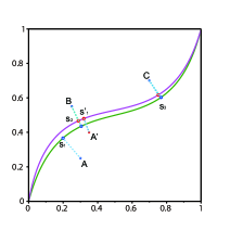
Figure 6: $A$, $B$ and $C$ are three objects to rank. $s_{1}$, $s_{2}$ and $s_{3}$ are scores given by the RPC (in green) of S-type shape in the figure. A different observation of $A$ (denoted by $A^{\prime}$) would give a different RPC (in pink) and thus a different ordering of objects.

TABLE I: RPC model can detect ordinal information contained in numerical observations in Fig. 6.

Object	$x_{1}$		$x_{2}$		RankAgg	RPC
	Value	Order	Value	Order		Score	Order
$A$	$0.3$	2	$0.25$	1	1.5	0.2329	1
$B$	$0.25$	1	$0.55$	2	1.5	0.3304	2
$C$	$0.7$	3	$0.7$	3	3	0.7300	3

(a) A group of bservations and ranking lists by different rules

Object	$x_{1}$		$x_{2}$		RankAgg	RPC
	Value	Order	Value	Order		Score	Order
$A^{\prime}$	$0.35$	2	$0.4$	1	1.5	0.3708	2
$B$	$0.25$	1	$0.55$	2	1.5	0.3431	1
$C$	$0.7$	3	$0.7$	3	3	0.7318	3

(b) Another group of bservations and ranking lists by different rules

Note: Different observations of objects would produce different ranking lists of objects. In (a), objects $A$, $B$ and $C$ can be ordered by their values on $x_{1}$ and $x_{2}$ respectively. Ranking aggregation (RankAgg) then produce a comprehensive ordering by Eq.(31). But it fails to distinguish $A$ and $B$ which have distinguishable observations while RPC can distinguish them. RPC can also detect the minor ordinal difference between objects. In (b), $A$ has a different observation from (a), which is denoted as $A^{\prime}$. Ranking lists keeps the same for RankAgg while RPC provides a different ordering.

For ranking task, some researchers prefer to aggregate many different ranking lists of the same set of objects in order to get a “better” order. For example, median rank aggregation [34] aggregates different orderings into a median rank with

$$\kappa(i)=\frac{\sum_{j=1}^{m}\tau_{j}(i)}{m},i=1,2,\cdots,n$$ (31)

where $\tau_{j}(i)$ is the location of object $i$ in ranking list $\tau_{j}$, $\tau_{j}$ is a permutation of $\{1,2,\cdots,n\}$ and $\kappa$ is the ordering of median rank aggregation. However, approaches of ranking aggregation suffers the difficulties of strict monotonicity and smoothness. Therefore, the ranking list is not very convincing. What’s more, aggregation merely combines the orderings and ignores the information delivered by numerical observations.

In contrast, RPC is modeled following all the five meta-rules which infers a reasonable ranking list. Moreover, RPC can detect the ordinal information embedded in the numerical observations, illustrated in Fig. 6. Consider to rank three objects $A$, $B$ and $C$ in a two-dimensional space in Fig. 6. Let their numerical observations on $x_{1}$ and $x_{2}$ be values shown in Table II(a). Objects can be ordered along with $x_{1}$ and $x_{2}$ respectively. Median rank aggregation [34] produces an ordering which can not distinguish $A$ and $B$ since they are in the paratactic place of the ranking list. In contrast, the RPC model produce the order $ABC$ where $A$ and $B$ are in a distinguishable order since RPC ranks objects based on their original observation data. If there is a different observation for one of objects, a different RPCwould produce a different ranking list while RankAgg remains the same. In Table II(b), a different observation of object $A$ is obtained, denoted as $A^{\prime}$. A different RPC is learned (the pink curve in Fig. 6) and gives the order $BA^{\prime}C$ (the last column of Table II(b)) which is different from the order in Table II(a). In summary, RPC is able to capture the ordinal information contained not only among ranking candidates but also in the individual observation.

6.2 Applications

Unsupervised ranking of multi-attribute observations of objects has a widely applications. The most significant application is to rank countries, journals and universities. Taking the journal ranking task for illustration, there have been many indices to rank journals, such as impact factor (IF) [39] and Eigenfactor [40]. Different indices reflect different aspects of journals and provide different ranking lists for journals. Thus, how to evaluate journals in a comprehensive way becomes a tough problem. RPC model is proposed as a new framework to attack the problem which provides an ordering along the “ranking skeleton” of data distribution. In this paper, we perform ranking tasks with RPCs to produce a comprehensive evaluation on three open access datasets of countries and journals with the open source software Scilab (5.4.1 version) on a Ubuntu 12.04 system with 4GB memory. Due to space limitation, we just list parts of their ranking lists (the full lists will be available when the paper is published).

6.2.1 Results on Life Qualities of Countries

TABLE II: Part of the ranking list for life qualities of countries.

Country	GDP1	LEB2	IMR3	Tuberculosis4	Elmap[8]		RPC
					Score	Order	Score	Order
Luxembourg	70014	79.56	6	4	0.892	1	1.0000	1
Norway	47551	80.29	3	3	0.647	2	0.8720	2
Kuwait	44947	77.258	11	10	0.608	3	0.8483	3
Singapore	41479	79.627	12	2	0.578	4	0.8305	4
United States	41674	77.93	2	7	0.575	5	0.8275	5
⋮	⋮	⋮	⋮	⋮	⋮	⋮	⋮	⋮
Moldova	2362	67.923	63	17	0.002	97	0.5139	96
Vanuatu	3477	69.257	37	31	0.011	96	0.5135	97
Suriname	7234	68.425	53	30	0.011	95	0.5133	98
Morocco	3547	70.443	44	36	0.002	98	0.5106	99
Iraq	3200	68.495	25	37	-0.002	100	0.5032	100
⋮	⋮	⋮	⋮	⋮	⋮	⋮	⋮	⋮
South Africa	8477	51.803	349	55	-0.652	167	0.0786	167
Sierra Leone	790	46.365	219	160	-0.664	169	0.0541	168
Djibouti	1964	54.456	330	88	-0.655	168	0.0524	169
Zimbabwe	538	41.681	311	68	-0.680	170	0.0462	170
Swaziland	4384	44.99	422	110	-0.876	171	0	171
$\mathbf{p}_{0}$	44713	81.218	2	0	-	-	-	-
$\mathbf{p}_{1}$	330	80.4	2	0	-	-	-	-
$\mathbf{p}_{2}$	330	59.7	33	43	-	-	-	-
$\mathbf{p}_{3}$	1581.824	41.68	290	151	-	-	-	-

• Gross Domestic Product per capita by Purchasing Power Parities, $per person;

• Life Expectancy at Birth, years;

• Infant Mortality Rate (per 1000 born);

• Infectious Tuberculosis, new cases per 100,000 of population, estimated.

• $\mathbf{p}_{j}(j=0,1,2,3)$ are control and end points of the RPC.

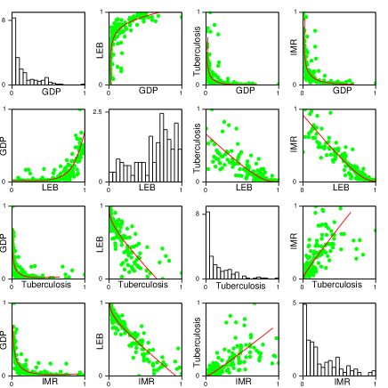
Figure 7: Two-dimensional display of data points and RPC for life qualities of countries. Green points are numerical observations and red curves are 2-dimensional projection of RPC.

Gorban et al. [8] ranked 171 countries by life qualities of people with data driven from GAPMINDER based on four indicators as in Example 2. For comparison, we also use the same four GAPMINDER indicators in [8]. The RPC learned by Algorithm 1 is shown in two-dimensional visualization in Fig. 7 and part of the ranking list is illustrated in Table II.

From Fig. 7, RPC portrays the data distributing trends with different shapes, including linearity and nonlinearity. For this task, ${\bm{\alpha}}=[1,1,-1,-1]^{T}$ for this task just as Example 2. $\bm{\alpha}$ also discovers the relationship between indicators for ranking. GDP is in the same direction with LEB, but in the opposite direction with IMR and Tuberculosis. In the beginning, a small amount of GDP increasing brings about tremendous increasing of LEB and tremendous decreasing of IMR and Tuberculosis. When GDP exceeds $14300 (0.2 as normalized value in Fig. 7) per person, increasing GDP does result in little LEB increase, so does IMR and Tuberculosis decrease. As a matter of fact, it is hard to improve further LEB, IMR and Tuberculosis when they are close to the limit of human evolution.

In Table II, control points provided by RPC learning algorithm (Algorithm 1) are listed in the bottom. $\mathbf{p}_{i}$ in the bottom is given in the original data space. Although the number of control points are set to two in addition to two end points, the number actually needed for each indicators is adapted automatically by learning. From Table II, $\mathbf{p}_{0}$ and $\mathbf{p}_{1}$ for IMR and Tuberculosis overlaps which means that three points are enough for a Bézier curve to depicts the skeleton of IMR and Tuberculosis. Two-dimensional visualizations in Fig. 7 tally with the statement above.

Gorban et al. [8] provided centered scores for countries, which is similar to the first PCA. But the zero score is assigned to no country such that no country is taken as the ranking reference. In addition, rankers would get into trouble to understand the ranking principle due to unknown parameter size. Therefore, the ranking list is hard to interpret for human understanding. Compared with Elmap [8], the presented RPC model follows all the five meta-rules. With these meta-rules as constraints, it achieves a better fitting performance in term of Mean Square Error ($90\%$ vs $86\%$ of explained variance). It produces scores in $[0,1]$ where 0 and 1 are the worst and the best reference respectively. Luxembourg with the best life quality provides a developing direction for countries below. Additionally, the RPC model is interpretable and easy to carry out in practice since there are just four points to determine the ranking list.

6.2.2 Results on Journal Ranking

TABLE III: Part of the ranking list for JCR2012 journals of computer sciences.

Title	Impact Factor (IF)		5-Year IF		Immediacy Index		Eigenfactor		Influence Score		RPC
	Score	Order	Score	Order	Score	Order	Score	Order	Score	Order	Score	Order
IEEE T PATTERN ANAL	4.795	7	6.144	5	0.625	26	0.05237	3	3.235	6	1.0000	1
ENTERP INF SYST UK	9.256	1	4.771	10	2.682	2	0.00173	230	0.907	86	0.9505	2
J STAT SOFTW	4.910	4	5.907	6	0.753	18	0.01744	20	3.314	4	0.9162	3
MIS QUART	4.659	8	7.474	2	0.705	21	0.01036	49	3.077	7	0.9105	4
ACM COMPUT SURV	3.543	21	7.854	1	0.421	56	0.00640	80	4.097	1	0.9092	5
$\vdots$	$\vdots$	$\vdots$	$\vdots$	$\vdots$	$\vdots$	$\vdots$	$\vdots$	$\vdots$	$\vdots$	$\vdots$	$\vdots$	$\vdots$
DECIS SUPPORT SYST	2.201	51	3.037	43	0.196	169	0.00994	52	0.864	93	0.4701	65
COMPUT STAT DATA AN	1.304	156	1.449	180	0.415	61	0.02601	11	0.918	83	0.4665	66
IEEE T KNOWL DATA EN	1.892	82	2.426	72	0.217	152	0.01256	37	1.129	55	0.4616	67
MACH LEARN	1.467	133	2.143	96	0.373	70	0.00638	81	1.528	20	0.4490	68
IEEE T SYST MAN CY A	2.183	53	2.44	68	0.465	46	0.00728	69	0.767	111	0.4466	69
$\vdots$	$\vdots$	$\vdots$	$\vdots$	$\vdots$	$\vdots$	$\vdots$	$\vdots$	$\vdots$	$\vdots$	$\vdots$	$\vdots$	$\vdots$

We also apply RPC model to rank journals with data accessable from the Web of Knowledge which is affiliated to Thomson Reuters. Thomson Reuters publishes annually Journal Citation Reports (JCR) which provide information about academic journals in the sciences and social sciences. JCR2012 reports citation information with indicators of Impact Factor, 5-year Impact Factor, Immediacy Index, Eigenfactor Score, and Article Influence Score. After journals with data missing are removed from the data table (58 out of 451), RPC model tries to provide a comprehensive ranking list of journals in the categories of computer science: artificial intelligence, cybernetics, information systems, interdisciplinary applications, software engineering, theory and methods. Table III illustrates the ranking list of journals produced by RPC model based on JCR2012. Two-dimensional visualization of the RPC is shown in Fig. 8.

For this ranking task, a journal will rank higher with a higher value for each indicator, that is ${\bm{\alpha}}=[1,1,1,1]$. Among all the indicators here, 5-year Impact Factor shows almost a linear relationship with the others. But Eigenfactor presents no clear relationship which means that it is calculated in a very different way from the other indicator. Actually, Eigenfactor works like PageRank [2] while the others take frequency count.

From Table III, IEEE Transactions on Knowledge and Data Engineering (TKDE) is ranked in a higher place than IEEE Transactions on Systems, Man, and Cybernetics-Part A (SMCA) although SMCA has a higher IF (2.183) than TKDE (1.892). The lower influence score (0.767) of SMCA brings it down the ranking list (vs. 1.129 for TKDE). Therefore, TKDE gets a higher comprehensive evaluating score and wins a higher ranking place in the ranking list. This means that one indicator does not tell the whole story of ranking lists. RPC produces a ranking list for journals taking account several indicators of different aspects.

Figure 8: Two-dimensional display of data points and RPC for JCR2012. Green points are numerical observations and red curves are 2-dimensional projection of RPC. (IF:Impact Factor, 5IF:5-Year IF, ImmInd:Immediacy Index, IS: Influence Score)

7 Conclusions

Ranking and its tools have and will have an increasing impact on the behavior of human, either positively or negatively. However, those ranking activities are still facing many challenges which have greatly restrained to the rational design and utilization of ranking tools. Generally, ranking in practice is an unsupervised task which encounters a critical challenge that there is no ground truth to evaluate the provided lists. PageRank [2] is an effective unsupervised ranking model for ranking candidates with a link-structure. However, it does not work for numerical observations on multiple attributes of objects.

It is well known that domain knowledge can always improve the data mining performance. We try to attack unsupervised ranking problems by domain knowledge about ranking. Motivated by [13, 16], five meta-rules as ranking knowledge are presented and are regarded as constraints to ranking models. They are scale and translation invariance, strict monotonicity, linear/nonlinear capacities, smoothness and explicitness of parameter size. They can also be capable of assessing the ranking performance of different models. Enlightened by [14, 8], we propose a ranking model with a principal curve which is parametrically formulated with a cubic Bézier curve by restricting control points in the interior of the hypercube $[0,1]^{d}$. Control points are learned from the data distribution without human interventions. Applications in life qualities of countries and journals of computer sciences show that the proposed RPC model can produce reasonable ranking lists.

From an application view points, there are many indicators for ranking objects. RPC can also be used to do feature selection which is one part of our future works.

Appendix A Principal Curves

Given a dataset $\mathbf{X}=(\mathbf{x_{1}},\mathbf{x_{2}},\cdots,\mathbf{x_{n}})$, $\mathbf{x}_{i}\in{\mathbf{R}^{d}}$, a principal curve summarizes the data with a smooth curve instead of a straight line in the first PCA

$$\mathbf{x}=\mathbf{f}(s)+{\bm{\varepsilon}}$$ (A-1)

where $\mathbf{f}(s)=(f_{1}(s),f_{2}(s),\cdots,f_{d}(s))\in{\mathbf{R}^{d}}$ and $s\in{\mathbf{R}}$. The principal curve $\mathbf{f}$ was originally defined by Hastie and Stuetzle [10] as a smooth ($C^{\infty}$) unit-speed ($\|\mathbf{f}^{\prime\prime}\|^{2}=1$) one-dimensional manifold in $\mathbf{R}^{d}$ satisfying the self-consistence condition

$$\mathbf{f}(s)=E\left(\left.\mathbf{x}\right|s_{\mathbf{f}}(\mathbf{x})=s\right)$$

where $s=s_{\mathbf{f}}(\mathbf{x})\in{\mathbf{R}}$ is the largest value so that $\mathbf{f}(s)$ has the minimum distance from $\mathbf{x}$. Mathematically, $s_{\mathbf{f}}(\mathbf{x})$ is formulated as [10]

$$s_{\mathbf{f}}(\mathbf{x})=\sup\left\{s:\|\mathbf{x}-\mathbf{f}(s)\|=\inf_{s}\|\mathbf{x}-\mathbf{f}(s)\|\right\}.$$ (A-2)

In other words, a curve $\mathbf{f}:\mathbf{R}\mapsto\mathbf{R}^{d}$ is called a principal curve if it minimizes the expected squared distance between $\mathbf{x}$ and $\mathbf{f}$ which is denoted by [11]

$$J(\mathbf{f})=E\left(\inf_{s}\|\mathbf{x}-\mathbf{f}(s)\|^{2}\right)=E\|\mathbf{x}-\mathbf{f}(s_{\mathbf{f}}(\mathbf{x}))\|^{2}.$$ (A-3)

As an one-dimensional principal manifold, the principal curve has a wide applications (e.g. [36]) due to its simpleness. Following Hastie and Stuetzle [10], researchers afterwards have proposed a variety of principal curve definitions and learning algorithms to perform different tasks [26, 11, 29, 19]. But most of them tried to first approximate the principal curve first with a polyline [11] and then smooth it to meet the requirement for smoothness [10] of the principal curve. Therefore, the expression of the principal curve is not explicit and results in a ‘black-box’ which is hard to interpret. The other definitions of principal curves [30, 27] employed Gaussian mixture model to generally formulate the principal curve which brings model bias and makes interpretation even harder. When the principal curve is used to perform a ranking task, it should be modeled to be a ‘white-box’ which can be well interpreted for its provided ranking lists.

Appendix B Proof of Theorem 2

If $\nabla\varphi(\mathbf{x})\succ\mathbf{0}$, $\varphi$ is strictly monotone by Theorem 1. Regarding that the ranking candidates is totally ordered, there is a one-to-one correspondence between ranking items in $\mathbf{R}^{d}$ and $\mathbf{rang}\varphi$. Otherwise, $s=\varphi(\mathbf{x}_{0})$ and $s=\varphi(\mathbf{x}_{0}+\triangle\mathbf{x})$ both hold for some $\mathbf{x}_{0}\in\mathbf{dom}\varphi$. In this case, $\left.\nabla\varphi(\mathbf{x})\right|_{\mathbf{x}=\mathbf{x}_{0}}=\mathbf{0}$ which contradicts the assumption $\nabla\varphi(\mathbf{x})\succ\mathbf{0}$ holds for all $\mathbf{x}\in\mathbf{dom}\varphi$.

By Lemma 1 and the one-to-one correspondence, there exists an inverse mapping $\mathbf{f}:\mathbf{rang}\varphi\mapsto\mathbf{dom}\varphi$ such that $\mathbf{x}=\mathbf{f}(s)$. By strict monotonicity (Eq.(1)) and the one-to-one correspondence, we have

$$\mathbf{x}_{1}\preceq\mathbf{x}_{2},\quad\mathbf{x}_{1}\neq\mathbf{x}_{2}\Longleftrightarrow s_{1}<s_{2}$$ (B-1)

Thus, $\nabla\mathbf{f}(s)\succ\mathbf{0}$ holds for $s\in\mathbf{rang}\varphi$. $\hfill\square$

Appendix C Proof of RPC Existence (Theorem 3)

Proof. Assume $\mathbf{U}=[0,1]$ and $C(\mathbf{U})$ denotes the set of all continuous function $\mathbf{f}:\mathbf{U}\mapsto[0,1]^{d}\subseteq{\mathbf{R}^{d}}$ embracing all possible observations of $\mathbf{x}$. The uniform metric is defined as

$$D(\mathbf{f},\mathbf{g})=\sup_{0\leq s\leq 1}\|{\mathbf{f}(s)-\mathbf{g}(s)}\|,\quad\forall\mathbf{f},\mathbf{g}\in{C(\mathbf{U})}.$$ (C-1)

It is easy to see $(C(\mathbf{U}),D)$ is a complete metric space [21].

Let $\mathbf{\varGamma}=\left\{\mathbf{f}(s):\mathbf{f}(s)=\mathbf{PMz},\mathbf{P}\in{\Theta}\right\}\subseteq{C(\mathbf{U})}$, where $\Theta\in[0,1]^{4}$ is the convex hull of $\mathbf{x}$. With the Frobenius norm, $\Theta$ is a sequentially compact set so that for any given sequence in $\Theta$ there exists a subsequence $\mathbf{P}^{(t)}$ converging uniformly to an $\mathbf{P}^{*}\in[0,1]^{d}$ [21] with

$$\|\mathbf{P}^{(t)}-\mathbf{P}^{*}\|_{F}\hskip 5.69046pt\rightarrow 0$$ (C-2)

Let $\mathbf{p}_{0}=\frac{1}{2}(\mathbf{1}-\bm{\alpha})$ and $\mathbf{p}_{3}=\frac{1}{2}(\mathbf{1}+\bm{\alpha})$. Then we have a sequence $\mathbf{f}^{(t)}(s)$ converging uniformly to $\mathbf{f}^{*}(s)$:

$$D\left(\mathbf{f}^{(t)}(s),\mathbf{f}^{*}(s)\right)=\sup_{0\leq s\leq 1}\|{\mathbf{f}^{(t)}(s)-\mathbf{f}^{*}(s)}\|$$ (C-3)

$$\leq \sup_{0\leq s\leq 1}\|\mathbf{P}^{(t)}-\mathbf{P}^{*}\|_{F}\|\mathbf{Mz}\|$$ (C-4)

$$= \|\mathbf{P}^{(t)}-\mathbf{P}^{*}\|_{F}\hskip 5.69046pt\rightarrow 0$$ (C-5)

where $\|\mathbf{Mz}\|=1$. By Proposition 1, $\mathbf{f}^{(t)}(s)$ is a curve sequence of strictly monotonicity and converges to $\mathbf{f}^{*}(s)$.

Assuming the converging sequence $\mathbf{f}^{(t)}(s)$ makes $J(\mathbf{P}^{(t)})\geq{J(\mathbf{P}^{*})}$ for fixed $\mathbf{x}\in\mathbf{R}^{d}$,

$$J(\mathbf{P}^{(t)})-J(\mathbf{P}^{*})$$ (C-6)

$$= \|\mathbf{x}-\mathbf{f}^{(t)}(s)\|^{2}-\|\mathbf{x}-\mathbf{f}^{*}(s)\|^{2}$$

$$\leq \left(\|\mathbf{x}-\mathbf{f}^{(t)}(s)\|+\|\mathbf{x}-\mathbf{f}^{*}(s)\|\right)\|\mathbf{f}^{(t)}(s)-\mathbf{f}^{*}(s)\|$$ (C-8)

$$\rightarrow 0$$

and therefore

$$E\left(J(\mathbf{P}^{(t)})-J(\mathbf{P}^{*})\right)\hskip 5.69046pt\rightarrow 0.$$ (C-9)

Finally, we complete the proof. $\hfill\square$

Appendix D Proof of Convergence (Proposition 2)

Proof: First of all, $\mathbf{P}^{(t)}$ generated by Richardson method has been proved to converge [37]. Assume $\mathbf{P}^{(t)}\rightarrow{\mathbf{P}^{*}}$, and $\mathbf{s}^{(t)}$ and $\mathbf{s}^{*}$ are the corresponding score vectors calculated by Eq.(23). Note that the item $\mathbf{P}^{(t+1)}-\mathbf{P}^{(t)}$ is in the descending direction of $J$ in Eq.(28). So we get that

$$J(\mathbf{P}^{(t)},\mathbf{s}^{(t)})\geq J(\mathbf{P}^{(t+1)},\mathbf{s}^{(t)}).$$ (D-1)

Then with the control points $\mathbf{P}^{(t+1)}$, $\mathbf{s}^{(t+1)}$ minimizes the summed orthogonal distance

$$J(\mathbf{P}^{(t+1)},\mathbf{s}^{(t)})\geq J(\mathbf{P}^{(t+1)},\mathbf{s}^{(t+1)}).$$ (D-2)

Thus we get

$$J(\mathbf{P}^{(t)},\mathbf{s}^{(t)})\geq J(\mathbf{P}^{(t+1)},\mathbf{s}^{(t+1)}).$$ (D-3)

Finally, by Theorem 3 the sequence $\{J(\mathbf{P}^{(t)},\mathbf{s}^{(t)})\}$ converges to its infimum $\{J(\mathbf{P}^{*},\mathbf{s}^{*})\}$ as $s\rightarrow\infty$. $\hfill\square$

References

- [1] H. Li, “A Short Introduction to Learning to Rank”, IEICE Trans. Inf. Syst., vol. E94-D, no. 10, pp. 1-9, 2011.
- [2] S. Brin and L. Page, “The Anatomy of a Large-Scale Hypertextual Web Search Engine”, Computer Networks, vol. 30, no. 1-7, pp. 107-117, 1998.
- [3] D. Zhou, J. Weston, A. Gretton, O. Bousquet, and B. Schölkopf, “Ranking on Data Manifolds”, Advances in Neural Information Processing Systems 16, S. Thrun, L. Saul, and B. Schölkopf, eds., MIT Press, 2004.
- [4] B. Xu, J. Bu, C. Chen, D. Cai, X. He, W. Liu, and J. Luo, “Efficient manifold ranking for image retrieval”, Proc. 34th Int’l ACM SIGIR Conf. Research and Development in Information Retrieval, pp. 525-534, 2011.
- [5] C. Bishop, Pattern Recognition and Machine Learning, New York: Springer, 2006.
- [6] I. Guyon and A. Elisseeff, “An Introduction to Variable and Feature Selection”, J. Mach. Learn. Res., vol. 3, pp. 1157-1182, 2003.
- [7] A. Klementiev, D. Roth, K. Small, and I. Titov, “Unsupervised Rank Aggregation with Domain-Specific Expertise”, Proc. 20th Int’l Joint Conf. Artifical Intell., pp. 1101-1106, 2009.
- [8] A.Y. Zinovyev and A.N. Gorban, “Nonlinear Quality of Life Index”[EB/OL], New York, http://arxiv.org/abs/1008.4063, 2010.
- [9] A. Vasuki, “A Review of Vector Quantization Techiniques”, IEEE Potentials, vol. 25, no. 4, pp. 39-47, 2006.
- [10] T. Hastie and W. Stuetzle, “Principal Curves”, J. Amer. Stat. Assoc., vol. 84, no. 406, pp. 502-516, 1989.
- [11] B. Kégl, A. Krzyżak, T. Linder, and K. Zeger, “Learning and Design of Principal Curves”, IEEE Trans. Pattern Anal. Mach. Intell., vol. 22, no. 3, pp. 281-297, 2000.
- [12] P. Gould, “Letting the Data Speak for Themselves”, Assoc. Amer. Geog. USA, vol. 71, no. 2, 1981.
- [13] B.-G. Hu, H.B. Qu, Y. Wang, and S.H. Yang, “A Generalized-Constraint Neural Network model: Associating Partially Known Relationships for Nonlinear Regression”, Inf. Sci., vol. 179, pp. 1929-1943, 2009.
- [14] B.-G. Hu, G.K.I Mann, and R.G. Gosine, “Control curve design for nonlinear (or fuzzy) proportional actions using spline-based functions”, Automatica, vol. 34, no. 9, pp. 1125-1133, 1998.
- [15] H. Daniels and M. Velikova, “Monotone and Partially Monotone Neural Networks”, IEEE Trans. Neural Networks, vol. 21, no. 6, pp. 906-917, 2010.
- [16] W. Kotłowski and R. Słowiński, “On Nonparametric Ordinal Classification with Monotonicity Constraints”, IEEE Trans. Knowl. Data Engineering, vol. 25, no. 11, pp. 2576-2589, 2013.
- [17] Y. Zhang, W. Zhang, J. Pei, X. Lin, Q. Lin, and A. Li, “Consensus-Based Ranking of Multivalued Objects: A Generalized Borda Count Approach”, IEEE Trans. Knowl. Data Engineering, vol. 26, no. 1, pp. 83-96, 2014.
- [18] X.Q. Cheng, P. Du, J.F. Guo, X.F. Zhu, and Y.X. Chen, “Ranking on Data Manifold with Sink Points”, IEEE Trans. Knowl. Data Engineering, vol. 25, no. 1, pp. 177-191, 2013.
- [19] A.N. Gorban and A.Y. Zinovyev, “Chapter 2: Principal Graphs and Manifolds”, Handbook of Research on Machine Learning Applications and Trends: Algorithms, Methods, and Techiniques, E.S. Olivas, J.D.M. Guerrero, M.M. Sober, J.R.M. Benedito, A.J.S. López, eds., New York: Inf. Sci. Ref., vol. 1, pp. 28-59, 2010.
- [20] T.A. Pastva, “Bézier Curve Fitting”, master’s thesis, Naval Postgraduate School, 1998.
- [21] S. Boyd and L. Vandenberghe, Convex Optimization, New York: Camb. Univ. Press, 2004.
- [22] H.A. Priestley, “Chapter 2: Ordered Sets and Complete Lattices-a Primer for Computer Science”, Algebraic and Coalgebraic Methods in the Mathematics of Program Construction, R. Backhouse, R. Crole, J. Jibbons, eds., LNCS 2297, pp. 21-78, 2002.
- [23] P.M. Fitzpatrick, Advanced Calculus, CA: Thomson Brooks/Cole, 2006.
- [24] A. Cambibi, D.T. Luc, and L. Martein. “Order-Preserving Transformations and Applications”, J. Optimization Theory Applications, vol. 118, no. 2, pp. 275-293, 2003.
- [25] T.W. Anderson, An Introduction to Multivariate Statistical Analysis, New Jersey: John Wiley & Sons, Inc. 2003.
- [26] J.D. Banfield and A.E. Raftery, “Ice Floe Identification in Satellite Images Using Mathematical Morphology and Clustering about Pincipal Curves”, J. Amer. Stat. Assoc., vol. 87, no. 417, pp. 7-16, 1992.
- [27] P. Delicado, “Another look at principal curves and surfaces”, J. Multivariate Anal., vol. 77, no. 1, pp. 84-116, 2001.
- [28] K. Chang and J. Ghosh, “A Unified Model for Probabilistic Principal Surfaces”, IEEE Trans. Pattern Anal. Mach. Intell., vol. 23, no. 1, pp. 22-41, 2001.
- [29] J. Einbeck, G. Tutz, and L. Evers, “Local Principal Curves”, Stat. and Comput., vol. 15, no. 4, pp. 301-313, 2005
- [30] R. Tibshirani, “Principal Curves Revisited”, Stat. and Comput., vol. 2, no. 4, pp. 183-190, 1992.
- [31] G. Farin, Curves and Surfaces for Computer Aided Geometric Design (4th Edition), California: Acad. Press, Inc., 1997.
- [32] M. A. Jenkins and J. F. Traub, “A Three-Stage Algorithm for Real Polynomials Using Quadratic Iteration”, SIAM J. Numer. Anal., vol. 7, no. 44, pp. 545–566, 1970.
- [33] M.S. Bazaraa, H.D. Sherali, and C.M. Shetty, Nonlinear Programming: Theory and Algorithms, New Jersey, Hoboken: John Wiley & Sons, Inc., 2006.
- [34] C. Dwork, R. Kumar, M. Naor, and D. Sivakumar, “Rank Aggregation Methods for the Web”, Proc. 10th Int’l Conf. World Wide Web, pp. 613-622, 2001.
- [35] R.A. Roger and C.R. Johnson, Matrix Analysis, New York: Camb. Univ. Press, 1985.
- [36] J.P. Zhang, X.D. Wang, U.Kruger, F.Y. Wang, “Principal Curve Algorithms for Partitioning High-Dimensional Data Spaces”, IEEE Trans. Neural Networks, vol. 22, no. 3, pp. 367-380, 2011.
- [37] L.F. Richardson, “The approximate arithmetical solution by finite differences of physical problems involving differential equations, with an application to the stresses in a masonry dam”, Philos. Trans. Roy. Soc. London Ser. A, vol. 210, pp. 307-357, 1910.
- [38] G. H. Golub and C. F. van Loan, Matrix Computations, 3rd ed., Baltimore, MD: Johns Hopkins, 1996.
- [39] E. Garfield, “The History and Meaning of the Journal Impact Factor”, J. Amer. Med. Assoc., vol. 295, no. 1, pp. 90-93, 2006.
- [40] C.T. Bergstrom, J.D. West, M.A. Wiseman,“The Eigenfactor Metrics”, J. of Neuroscience, vol. 28, no. 45, pp. 11433-11434, 2008.