Off-Policy General Value Functions to Represent Dynamic Role Assignments in RoboCup 3D Soccer Simulation

Abstract

Collecting and maintaining accurate world knowledge in a dynamic, complex, adversarial, and stochastic environment such as the RoboCup 3D Soccer Simulation is a challenging task. Knowledge should be learned in real-time with time constraints. We use recently introduced Off-Policy Gradient Descent algorithms within Reinforcement Learning that illustrate learnable knowledge representations for dynamic role assignments. The results show that the agents have learned competitive policies against the top teams from the RoboCup 2012 competitions for three vs three, five vs five, and seven vs seven agents. We have explicitly used subsets of agents to identify the dynamics and the semantics for which the agents learn to maximize their performance measures, and to gather knowledge about different objectives, so that all agents participate effectively and efficiently within the group.

ynamic Role Assignment Function, Reinforcement Learning, GQ($\lambda$), Greedy-GQ($\lambda$), Off-PAC, Off-Policy Prediction and Control, and RoboCup 3D Soccer Simulation.

1 Introduction

The RoboCup 3D Soccer Simulation environment provides a dynamic, real-time, complex, adversarial, and stochastic multi-agent environment for simulated agents. The simulated agents formalize their goals in two layers: 1. the physical layers, where controls related to walking, kicking etc. are conducted; and 2. the decision layers, where high level actions are taken to emerge behaviors. In this paper, we investigate a mechanism suitable for decision layers to use recently introduced Off-Policy Gradient Decent Algorithms in Reinforcement Leaning (RL) that illustrate learnable knowledge representations to learn about a dynamic role assignment function.

In order to learn about an effective dynamic role assignment function, the agents need to consider the dynamics of agent-environment interactions. We consider these interactions as the agent’s knowledge. If this knowledge is represented in a formalized form (e.g., first-order predicate logic) an agent could infer many aspects about its interactions consistent with that knowledge. The knowledge representational forms show different degrees of computational complexities and expressiveness [22]. The computational requirements increase with the extension of expressiveness of the representational forms. Therefore, we need to identify and commit to a representational form, which is scalable for on-line learning while preserving expressivity. A human soccer player knows a lot of information about the game before (s)he enters onto the field and this prior knowledge influences the outcome of the game to a great extent. In addition, human soccer players dynamically change their knowledge during games in order to achieve maximum rewards. Therefore, the knowledge of the human soccer player is to a certain extent either predictive or goal-oriented. Can a robotic soccer player collect and maintain predictive and goal-oriented knowledge? This is a challenging problem for agents with time constraints and limited computational resources.

We learn the role assignment function using a framework that is developed based on the concepts of Horde, the real-time learning methodology, to express knowledge using General Value Functions (GVFs) [22]. Similar to Horde’s sub-agents, the agents in a team are treated as independent RL sub-agents, but the agents take actions based on their belief of the world model. The agents may have different world models due to noisy perceptions and communication delays. The GVFs are constituted within the RL framework. They are predictions or off-policy controls that are answers to questions. For example, in order to make a prediction a question must be asked of the form “If I move in this formation, would I be in a position to score a goal?”, or “What set of actions do I need to block the progress of the opponent agent with the number 3?”. The question defines what to learn. Thus, the problem of prediction or control can be addressed by learning value functions. An agent obtains its knowledge from information communicated back and forth between the agents and the agent-environment interaction experiences.

There are primarily two algorithms to learn about the GVFs, and these algorithms are based on Off-Policy Gradient Temporal Difference (OP-GTD) learning: 1. with action-value methods, a prediction question uses GQ($\lambda$) algorithm [8], and a control or a goal-oriented question uses Greedy-GQ($\lambda$) algorithm [9]. These algorithms learned about a deterministic target policies and the control algorithm finds the greedy action with respect to the action-value function; and 2. with policy-gradient methods, a goal-oriented question can be answered using Off-Policy Actor-Critic algorithm [24], with an extended state-value function, GTD($\lambda$) [7], for GVFs. The policy gradient methods are favorable for problems having stochastic optimal policies, adversarial environments, and problems with large action spaces. The OP-GTD algorithms possess a number of properties that are desirable for on-line learning within the RoboCup 3D Soccer Simulation environment: 1. off-policy updates; 2. linear function approximation; 3. no restrictions on the features used; 4. temporal-difference learning; 5. on-line and incremental; 6. linear in memory and per-time-step computation costs; and 7. convergent to a local optimum or equilibrium point [23, 9].

In this paper, we present a methodology and an implementation to learn about a dynamic role assignment function considering the dynamics of agent-environment interactions based on GVFs. The agents ask questions and approximate value functions answer to those questions. The agents independently learn about the role assignment functions in the presence of an adversary team. Based on the interactions, the agents may have to change their roles in order to continue in the formation and to maximize rewards. There is a finite number of roles that an agent can commit to, and the GVFs learn about the role assignment function. We have conducted all our experiments in the RoboCup 3D Soccer Simulation League Environment. It is based on the general purpose multi-agent simulator SimSpark. The robot agents in the simulation are modeled based on the Aldebaran NAO robots. Each robot has 22 degrees of freedom. The agents communicate with the server through message passing and each agent is equipped with noise free joint perceptors and effectors. In addition to this, each agent has a noisy restricted vision cone of $120^{o}$. Every simulation cycle is limited to $20~{}ms$, where agents perceive noise free angular measurements of each joint and the agents stimulate the necessary joints by sending torque values to the simulation server. The vision information from the server is available every third cycle ($60~{}ms$), which provides spherical coordinates of the perceived objects. The agents also have the option of communicating with each other every other simulation cycle ($40~{}ms$) by broadcasting a $20~{}bytes$ message. The simulation league competitions are currently conducted with 11 robots on each side (22 total).

The remainder of the paper is organized as follows: In Section 2, we briefly discuss knowledge representation forms and existing role assignment formalisms. In Section 3, we introduce GVFs within the context of robotic soccer. In Section 4, we formalize our mechanisms of dynamic role assignment functions within GVFs. In Section 5, we identify the question and answer functions to represent GVFs, and Section 6 presents the experiment results and the discussion. Finally, Section 7 contains concluding remarks, and future work.

2 Related Work

One goal of multi-agent systems research is the investigation of the prospects of efficient cooperation among a set of agents in real-time environments. In our research, we focus on the cooperation of a set of agents in a real-time robotic soccer simulation environment, where the agents learn about an optimal or a near-optimal role assignment function within a given formation using GVFs. This subtask is particularly challenging compared to other simulation leagues considering the limitations of the environment, i.e. the limited locomotion capabilities, limited communication bandwidth, or crowd management rules. The role assignment is a part of the hierarchical machine learning paradigm [20, 19], where a formation defines the role space. Homogeneous agents can change roles flexibly within a formation to maximize a given reward function.

RL framework offerers a set of tools to design sophisticated and hard-to-engineer behaviors in many different robotic domains (e.g., [4]). Within the domain of robotic soccer, RL has been successfully applied in learning the keep-away subtask in the RoboCup 2D [18] and 3D [16] Soccer Simulation Leagues. Also, in other RoboCup leagues, such as the Middle Size League, RL has been applied successfully to acquire competitive behaviors [2]. One of the noticeable impact on RL is reported by the Brainstormers team, the RoboCup 2D Simulation League team, on learning different subtasks [14]. A comprehensive analysis of a general batch RL framework for learning challenging and complex behaviors in robot soccer is reported in [15]. Despite convergence guarantees, Q($\lambda$) [21] with linear function approximation has been used in role assignment in robot soccer [5] and faster learning is observed with the introduction of heuristically accelerated methods [3]. The dynamic role allocation framework based on dynamic programming is described in [6] for real-time soccer environments. The role assignment with this method is tightly coupled with the agent’s low-level abilities and does not take the opponents into consideration. On the other hand, the proposed framework uses the knowledge of the opponent positions as well as other dynamics for the role assignment function.

Sutton et al. [22] have introduced a real-time learning architecture, Horde, for expressing knowledge using General Value Functions (GVFs). Our research is built on Horde to ask a set of questions such that the agents assign optimal or near-optimal roles within formations. In addition, following researches describe methods and components to build strategic agents: [1] describes a methodology to build a cognizant robot that possesses vast amount of situated, reversible and expressive knowledge. [11] presents a methodology to “next” in real time predicting thousands of features of the world state, and [10] presents methods predict about temporally extended consequences of a robot’s behaviors in general forms of knowledge. The GVFs are successfully used (e.g., [13, 25]) for switching and prediction tasks in assistive biomedical robots.

3 Learnable knowledge representation for Robotic Soccer

Recently, within the context of the RL framework [21], a knowledge representation language has been introduced, that is expressive and learnable from sensorimotor data. This representation is directly usable for robotic soccer as agent-environment interactions are conducted through perceptors and actuators. In this approach, knowledge is represented as a large number of approximate value functions each with its 1. own policy; 2. pseudo-reward function; 3. pseudo-termination function; and 4. pseudo-terminal-reward function[22]. In continuous state spaces, approximate value functions are learned using function approximation and using more efficient off-policy learning algorithms. First, we briefly introduce some of the important concepts related to the GVFs. The complete information about the GVFs are available in [22, 8, 9, 7]. Second, we show its direct application to simulated robotic soccer.

3.1 Interpretation

The interpretation of the approximate value function as a knowledge representation language grounded on information from perceptors and actuators is defined as:

Definition 1

The knowledge expressed as an approximate value function is true or accurate, if its numerical values matches those of the mathematically defined value function it is approximating.

Therefore, according to the Definition (1), a value function asks a question, and an approximate value function is the answer to that question. Based on prior interpretation, the standard RL framework extends to represent learnable knowledge as follows. In the standard RL framework [21], let the agent and the world interact in discrete time steps $t=1,2,3,\ldots$. The agent senses the state at each time step $S_{t}\in\mathcal{S}$, and selects an action $A_{t}\in\mathcal{A}$. One time step later the agent receives a scalar reward $R_{t+1}\in\mathbb{R}$, and senses the state $S_{t+1}\in\mathcal{S}$. The rewards are generated according to the reward function $r:S_{t+1}\rightarrow\mathbb{R}$. The objective of the standard RL framework is to learn the stochastic action-selection policy $\pi:\mathcal{S}\times\mathcal{A}\rightarrow[0,1]$, that gives the probability of selecting each action in each state, $\pi(s,a)=\pi(s|a)=\mathcal{P}(A_{t}=a|S_{t}=s)$, such that the agent maximizes rewards summed over the time steps. The standard RL framework extends to include a terminal-reward-function, $z:\mathcal{S}\rightarrow\mathbb{R}$, where $z(s)$ is the terminal reward received when the termination occurs in state $s$. In the RL framework, $\gamma\in[0,1)$ is used to discount delayed rewards. Another interpretation of the discounting factor is a constant probability of $1-\gamma$ termination of arrival to a state with zero terminal-reward. This factor is generalized to a termination function $\gamma:\mathcal{S}\rightarrow[0,1]$, where $1-\gamma(s)$ is the probability of termination at state $s$, and a terminal reward $z(s)$ is generated.

3.2 Off-Policy Action-Value Methods for GVFs

The first method to learn about GVFs, from off-policy experiences, is to use action-value functions. Let $G_{t}$ be the complete return from state $S_{t}$ at time $t$, then the sum of the rewards (transient plus terminal) until termination at time $T$ is:

$$G_{t}=\sum_{k=t+1}^{T}r(S_{k})+z(S_{T}).$$

The action-value function is:

$$Q^{\pi}(s,a)=\mathbb{E}(G_{t}|S_{t}=s,A_{t}=a,A_{t+1:T-1}\sim\pi,T\sim\gamma),$$

where, $Q^{\pi}:\mathcal{S}\times\mathcal{A}\rightarrow\mathbb{R}$. This is the expected return for a trajectory started from state $s$, and action $a$, and selecting actions according to the policy $\pi$, until termination occurs with $\gamma$. We approximate the action-value function with $\hat{Q}:\mathcal{S}\times\mathcal{A}\rightarrow\mathbb{R}$. Therefore, the action-value function is a precise grounded question, while the approximate action-value function offers the numerical answer. The complete algorithm for Greedy-GQ($\lambda$) with linear function approximation for GVFs learning is as shown in Algorithm (1).

1:Initialize $w_{0}$ to $0$, and $\theta_{0}$ arbitrary.

2:Choose proper (small) positive values for $\alpha_{\theta}$, $\alpha_{w}$, and set values for $\gamma(.)\in(0,1]$, $\lambda(.)\in[0,1]$.

3:repeat

4:     Initialize $e=0$.

5:     Take $A_{t}$ from $S_{t}$ according to $\pi_{b}$, and arrive at $S_{t+1}$.

6:     Observe sample, ($S_{t},A_{t},r(S_{t+1}),z(S_{t+1}),S_{t+1},$) at time step $t$ (with their corresponding state-action feature vectors), where $\hat{\phi}_{t+1}=\phi(S_{t+1},A_{t+1}^{*}),A_{t+1}^{*}=\operatornamewithlimits{argmax}_{b}{\bf\theta}_{t}^{\mathrm{T}}\phi(S_{t+1},b)$.

7:     for each observed sample do

8:         $\delta_{t}\leftarrow r(S_{t+1})+(1-\gamma(S_{t+1}))z(S_{t+1})+\gamma(S_{t+1})\theta_{t}^{\mathrm{T}}\hat{\phi}_{t+1}-\theta_{t}^{\mathrm{T}}\phi_{t}$.

9:         If $A_{t}=A_{t}^{*}$, then $\rho_{t}\leftarrow\frac{1}{\pi_{b}(A_{t}^{*}|S_{t})}$; otherwise $\rho_{t}\rightarrow 0$.

10:         $e_{t}\leftarrow I_{t}\phi_{t}+\gamma(S_{t})\lambda(S_{t})\rho_{t}e_{t-1}$.

11:         $\theta_{t+1}\leftarrow\theta_{t}+\alpha_{\theta}[\delta_{t}e_{t}-\gamma(S_{t+1})(1-\lambda(S_{t+1}))(w_{t}^{\mathrm{T}}e_{t})\hat{\phi}_{t+1}]$.

12:         $w_{t+1}\leftarrow w_{t}+\alpha_{w}[\delta_{t}e_{t}-(w_{t}^{\mathrm{T}}\phi_{t})\phi_{t})]$.

13:     end for

14:until  each episode.

Algorithm 1 Greedy-GQ($\lambda$) with linear function approximation for GVFs learning [7].

The GVFs are defined over four functions: $\pi,\gamma,r,\mbox{and }z$. The functions $r\mbox{ and }z$ act as pseudo-reward and pseudo-terminal-reward functions respectively. Function $\gamma$ is also in pseudo form as well. However, $\gamma$ function is more substantive than reward functions as the termination interrupts the normal flow of state transitions. In pseudo termination, the standard termination is omitted. In robotic soccer, the base problem can be defined as the time until a goal is scored by either the home or the opponent team. We can consider a pseudo-termination has occurred when the striker is changed. The GVF with respect to a state-action function is defined as:

$$Q^{\pi,\gamma,r,z}(s,a)=\mathbb{E}(G_{t}|S_{t}=s,A_{t}=a,A_{t+1:T-1}\sim\pi,T\sim\gamma).$$

The four functions, $\pi,\gamma,r,\mbox{and }z$, are the question functions to GVFs, which in return defines the general value function’s semantics. The RL agent learns an approximate action-value function, $\hat{Q}$, using the four auxiliary functions $\pi,\gamma,r$ and $z$. We assume that the state space is continuous and the action space is discrete. We approximate the action-value function using a linear function approximator. We use a feature extractor $\mathcal{\phi}:S_{t}\times A_{t}\rightarrow\{0,1\}^{N},N\in\mathbb{N}$, built on tile coding [21] to generate feature vectors from state variables and actions. This is a sparse vector with a constant number of “1” features, hence, a constant norm. In addition, tile coding has the key advantage of real-time learning and to implement computationally efficient algorithms to learn approximate value functions. In linear function approximation, there exists a weight vector, $\theta\in\mathbb{R}^{N},N\in\mathbb{N}$, to be learned. Therefore, the approximate GVFs are defined as:

$$\hat{Q}(s,a,\theta)=\theta^{\mathrm{T}}\phi(s,a),$$

such that, $\hat{Q}:\mathcal{S}\times\mathcal{A}\times\mathbb{R}^{N}\rightarrow\mathbb{R}$. Weights are learned using the gradient-descent temporal-difference Algorithm (1) [7]. The Algorithm learns stably and efficiently using linear function approximation from off-policy experiences. Off-policy experiences are generated from a behavior policy, $\pi_{b}$, that is different from the policy being learned about named as target policy, $\pi$. Therefore, one could learn multiple target policies from the same behavior policy.

3.3 Off-Policy Policy Gradient Methods for GVFs

The second method to learn about GVFs is using the off-policy policy gradient methods with actor-critic architectures that use a state-value function suitable for learning GVFs. It is defined as:

$$V^{\pi,\gamma,r,z}(s)=\mathbb{E}(G_{t}|S_{t}=s,A_{t:T-1}\sim\pi,T\sim\gamma),$$

where, $V^{\pi,\gamma,r,z}(s)$ is the true state-value function, and the approximate GVF is defined as:

$$\hat{V}(s,v)=v^{\mathrm{T}}\phi(s),$$

where, the functions $\pi,\gamma,r,\mbox{and }z$ are defined as in the subsection (3.2). Since our the target policy $\pi$ is discrete stochastic, we use a Gibbs distribution of the form:

$$\pi(a|s)=\frac{e^{u^{\mathrm{T}}\phi(s,a)}}{\sum_{b}e^{u^{\mathrm{T}}\phi(s,b)}},$$

where, $\phi(s,a)$ are state-action features for state $s$, and action $a$, which are in general unrelated to state features $\phi(s)$, that are used in state-value function approximation. $u\in\mathbb{R}^{N_{u}},N_{u}\in\mathbb{N}$, is a weight vector, which is modified by the actor to learn about the stochastic target policy. The log-gradient of the policy at state $s$, and action $a$, is:

$$\frac{\nabla_{u}\pi(a|s)}{\pi(a|s)}=\phi(s,a)-\sum_{b}\pi(b|s)\phi(s,b).$$

The complete algorithm for Off-PAC with linear function approximation for GVFs learning is as shown in Algorithm (2).

1:Initialize $w_{0}$ to $0$, and $v_{0}$ and $u_{0}$ arbitrary.

2:Choose proper (small) positive values for $\alpha_{v}$, $\alpha_{w}$, $\alpha_{u}$, and set values for $\gamma(.)\in(0,1]$, $\lambda(.)\in[0,1]$.

3:repeat

4:     Initialize $e^{v}=0,\mbox{and }e^{u}=0$.

5:     Take $A_{t}$ from $S_{t}$ according to $\pi_{b}$, and arrive at $S_{t+1}$.

6:     Observe sample, ($S_{t},A_{t},r(S_{t+1}),z(S_{t+1}),S_{t+1}$) at time step $t$ (with their corresponding state ($\phi_{t},\phi_{t+1}$) feature vectors, where $\phi_{t}=\phi(S_{t})$).

7:     for each observed sample do

8:         $\delta_{t}\leftarrow r(S_{t+1})+(1-\gamma(S_{t+1}))z(S_{t+1})+\gamma(S_{t+1})v_{t}^{\mathrm{T}}\phi_{t+1}-v_{t}^{\mathrm{T}}\phi_{t}$.

9:         $\rho_{t}\leftarrow\frac{\pi(A_{t}|S_{t})}{\pi_{b}(A_{t}|S_{t})}$.

10:         Update the critic (GTD($\lambda$) algorithm for GVFs).

11:               $e^{v}_{t}\leftarrow\rho_{t}(\phi_{t}+\gamma(S_{t})\lambda(S_{t})e^{v}_{t-1})$.

12:               $v_{t+1}\leftarrow v_{t}+\alpha_{v}[\delta_{t}e^{v}_{t}-\gamma(S_{t+1})(1-\lambda(S_{t+1}))({e^{v}_{t}}^{\mathrm{T}}w_{t})\phi_{t+1}]$.

13:               $w_{t+1}\leftarrow w_{t}+\alpha_{w}[\delta_{t}e_{t}-(w_{t}^{\mathrm{T}}\phi_{t})\phi_{t})]$.

14:         Update the actor.

15:               $e^{u}_{t}\leftarrow\rho_{t}\left[\frac{\nabla_{u}\pi(A_{t}|S_{t})}{\pi(A_{t}|S_{t})}+\gamma(S_{t})\lambda(S_{t+1})e^{u}_{t-1}\right]$.

16:               $u_{t+1}\leftarrow u_{t}+\alpha_{u}\delta_{t}e^{u}_{t}$.

17:     end for

18:until  each episode.

Algorithm 2 Off-PAC with linear function approximation for GVFs learning [7, 24].

We are interested in finding optimal policies for the dynamic role assignment, and henceforth, we use Algorithms (1), and (2) for control purposes. We use linear function approximation for continuous state spaces, and discrete actions are used within options. Lastly, to summarize, the definitions of the question functions and the answer functions are given as:

Definition 2

The question functions are defined by:

1. $\pi:S_{t}\times A_{t}\rightarrow[0,1]$ 35mm (target policy is greedy w.r.t. learned value function);

2. $\gamma:S_{t}\rightarrow[0,1]$ 35mm (termination function);

3. $r:S_{t+1}\rightarrow\mathbb{R}$ 35mm (transient reward function); and

4. $z:S_{t+1}\rightarrow\mathbb{R}$ 35mm (terminal reward function).

Definition 3

The answer functions are defined by:

1. $\pi_{b}:S_{t}\times A_{t}\rightarrow[0,1]$ 35mm (behavior policy);

2. $I_{t}:S_{t}\times A_{t}\rightarrow[0,1]$ 35mm (interest function);

3. $\phi:S_{t}\times A_{t}\rightarrow\mathbb{R}^{N}$ 35mm (feature-vector function); and

4. $\lambda:S_{t}\rightarrow[0,1]$ 35mm (eligibility-trace decay-rate function).

4 Dynamic Role Assignment

A role is a specification of an internal or an external behavior of an agent. In our soccer domain, roles select behaviors of agents based on different reference criteria: the agent close to the ball becomes the striker. Given a role space, $\mathcal{R}=\{r_{1},\ldots,r_{n}\}$, of size $n$, the collaboration among $m\leq n$ agents, $\mathcal{A}=\{a_{1},\dots,a_{m}\}$, is obtained through formations. The role space consists of active and reactive roles. For example, the striker is an active role and the defender could be a reactive role. Given a reactive role, there is a function, $R\mapsto T$, that maps roles to target positions, $T$, on the field. These target positions are calculated with respect to a reference pose (e.g., ball position) and other auxiliary criteria such as crowd management rules. A role assignment function, $R\mapsto A$, provides a mapping from role space to agent space, while maximizing some reward function. The role assignment function can be static or dynamic. Static role assignments often provide inferior performance in robot soccer [6]. Therefore, we learn a dynamic role assignment function within the RL framework using off-policy control.

Figure 1: Primary formation, [17]

4.1 Target Positions with the Primary Formation

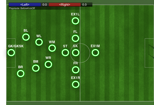
Within our framework, an agent can choose one role among thirteen roles. These roles are part of a primary formation, and an agent calculates the respective target positions according to its belief of the absolute ball position and the rules imposed by the 3D soccer simulation server. We have labeled the role space in order to describe the behaviors associated with them. Figure (1) shows the target positions for the role space before the kickoff state. The agent closest to the ball takes the striker role (SK), which is the only active role. Let us assume that the agent’s belief of the absolute ball position is given by $(x_{b},y_{b})$. Forward left (FL) and forward right (FR) target positions are offset by $(x_{b},y_{b})\pm(0,2)$. The extended forward left (EX1L) and extended forward right ((EX1R)) target positions are offset by $(x_{b},y_{b})\pm(0,4)$. The stopper (ST) position is given by $(x_{b}-2.0,y_{b})$. The extended middle (EX1M) position is used as a blocking position and it is calculated based on the closest opponent to the current agent. The other target positions, wing left (WL), wing right (WR), wing middle (WM), back left (BL), back right (BR), and back middle (BM) are calculated with respect to the vector from the middle of the home goal to the ball and offset by a factor which increases close to the home goal. When the ball is within the reach of goal keeper, the (GK) role is changed to goal keeper striker (GKSK) role. We slightly change the positions when the ball is near the side lines, home goal, and opponent goal. These adjustments are made in order to keep the target positions inside the field. We allow target positions to be overlapping. The dynamic role assignment function may assign the same role during the learning period. In order to avoid position conflicts an offset is added; the feedback provides negative rewards for such situations.

4.2 Roles to RL Action Mapping

The agent closest to the ball becomes the striker, and only one agent is allowed to become the striker. The other agents except the goalie are allowed to choose from twelve roles. We map the available roles to discrete actions of the RL algorithm. In order to use Algorithm 1, an agent must formulate a question function using a value function, and the answer function provides the solution as an approximate value function. All the agents formulate the same question: What is my role in this formation in order to maximize future rewards? All agents learn independently according to the question, while collaboratively aiding each other to maximize their future reward. We make the assumption that the agents do not communicate their current role. Therefore, at a specific step, multiple agents may commit to the same role. We discourage this condition by modifying the question as What is my role in this formation in order to maximize future rewards, while maintaining a completely different role from all teammates in all time steps?

Figure 2: State variable representation and the primary function. Some field lines are omitted due to clarity.

4.3 State Variables Representation

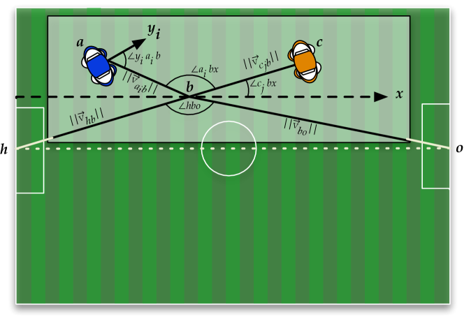
Figure 2 shows the schematic diagram of the state variable representation. All points and vectors in Figure 2 are defined with respect to a global coordinate system. $h$ is the middle point of the home goal, while $o$ is the middle point of the opponent goal. $b$ is the ball position. $\parallel$.$\parallel$ represents the vector length, while $\angle pqr$ represents the angle among three points $p,~{}q,\mbox{ and }r$ pivoted at $q$. $a_{i}$ represents the self-localized point of the $i=1,\ldots,11$ teammate agent. $y_{i}$ is some point in the direction of the robot orientation of teammate agents. $c_{j}$, $j=1,\ldots,11$, represents the mid-point of the tracked opponent agent. $x$ represents a point on a vector parallel to unit vector $e_{x}$. Using these labels, we define the state variables as:

$$\{\parallel\vec{v}_{hb}\parallel,\parallel\vec{v}_{bo}\parallel,\angle hbo,\{\parallel\vec{v}_{a_{i}b}\parallel,\angle y_{i}a_{i}b,\angle a_{i}bx\}_{i=n_{start}}^{n_{end}},\{\parallel\vec{v}_{c_{j}b}\parallel,\angle c_{j}bx,\}_{j=1}^{m_{max}}\}.$$

$n_{start}$ is the teammate starting id and $n_{end}$ the ending id. $m_{max}$ is the number of opponents considered. Angles are normalized to [$-\frac{\pi}{2},\frac{\pi}{2}$].

5 Question and Answer Functions

There are twelve actions available in each state. We have left out the striker role from the action set. The agent nearest to the ball becomes the striker. All agents communicate their belief to other agents. Based on their belief, all agents calculate a cost function and assign the closest agent as the striker. We have formulated a cost function based on relative distance to the ball, angle of the agent, number of teammates and opponents within a region near the ball, and whether the agents are active. In our formulation, there is a natural termination condition; scoring goals. With respect to the striker role assignment procedure, we define a pseudo-termination condition. When an agent becomes a striker, a pseudo-termination occurs, and the striker agent does not participate in the learning process unless it chooses another role. We define the question and answer functions as follows:

5.1 GVF Definitions for State-Action Functions

Question functions:

1. $\pi=$ greedy w.r.t. $\hat{Q}$,

2. $\gamma(.)=0.8$,

3. $r(.)=$ (a) the change of $x$ value of the absolute ball position; (b) a small negative reward of $0.01$ for each cycle; (c) a negative reward of $5$ is given to all agents within a radius of 1.5 meters;

4. $z(.)=$ (a) $+100$for scoring against opponent; (b) $-100$for opponent scoring; and

5. $\mbox{time step}=2$ seconds.

Answer functions:

1. $\pi_{b}=$ $\epsilon$-greedy w.r.t. target state-action function,

2. $\epsilon=0.05$,

3. $I_{t}(.)=1$,

4. $\phi(.,.)=$ (a) we use tile coding to formulate the feature vector. $n_{start}=2$ and $n_{end}=3,5,7$. $m_{max}=3,5,7$. Therefore, there are $18,28,30$ state variables. (b) state variable is independently tiled with 16 tilings with approximately each with $\frac{1}{16}$ generalization. Therefore, there are $288+1,448+1,608+1$ active tiles (i.e., tiles with feature 1) hashed to a binary vector dimension $10^{6}+1$. The bias feature is always active, and

5. $\lambda(.)=0.8$.

Parameters:
• 6mm 1. $\parallel{\bf{\theta}}\parallel=\parallel{\bf w}\parallel=10^{6}+1$; 2. $\parallel{\bf e}\parallel=2000$(efficient trace implementation); 6mm 3. $\alpha_{\theta}=\frac{0.01}{289},\frac{0.01}{449},\frac{0.01}{609}$; and 4. $\alpha_{w}=0.001\times\alpha_{\theta}$.

5.2 GVF for Gradient Descent Functions

Question functions:

1. $\pi=$ Gibbs distribution,

2. $\gamma(.)=0.9$,

3. $r(.)=$ (a) the change of $x$ value of the absolute ball position; (b) a small negative reward of $0.01$ for each cycle; (c) a negative reward of $5$ is given to all agents within a radius of 1.5 meters;

4. $z(.)=$ (a) $+100$for scoring against opponent; (b) $-100$for opponent scoring; and

5. $\mbox{time step}=2$ seconds.

Answer functions:

1. $\pi_{b}=$ the learned Gibbs distribution is used with a small perturbation. In order to provide exploration, with probability $0.01$, Gibbs distribution is perturbed using some $\beta$ value. In our experiments, we use $\beta=0.5$. Therefore, we use a behavior policy: $\frac{e^{u^{\mathrm{T}}\phi(s,a)+\beta}}{\sum_{b}e^{u^{\mathrm{T}}\phi(s,b)+\beta}}$

2. $\phi(.)=$ (a) the representations for the state-value function, we use tile coding to formulate the feature vector. $n_{start}=2$ and $n_{end}=3,5,7$. $m_{max}=3,5,7$. Therefore, there are $18,28,30$ state variables. (b) state variable is independently tiled with 16 tilings with approximately each with $\frac{1}{16}$ generalization. Therefore, there are $288+1,448+1,608+1$ active tiles (i.e., tiles with feature 1) hashed to a binary vector dimension $10^{6}+1$. The bias feature is always set to active;

3. $\phi(.,.)=$ (a) the representations for the Gibbs distribution, we use tile coding to formulate the feature vector. $n_{start}=2$ and $n_{end}=3,5,7$. $m_{max}=3,5,7$. Therefore, there are $18,28,30$ state variables. (b) state variable is independently tiled with 16 tilings with approximately each with $\frac{1}{16}$ generalization. Therefore, there are $288+1,448+1,608+1$ active tiles (i.e., tiles with feature 1) hashed to a binary vector dimension $10^{6}+1$. The hashing has also considered the given action. The bias feature is always set to active; and

4. $\lambda_{\mbox{critic}}(.)=\lambda_{\mbox{actor}}(.)=0.3$.

Parameters:
• 6mm 1. $\parallel{\bf{u}}\parallel=10^{6}+1$; 2. $\parallel{\bf{\theta}}\parallel=\parallel{\bf w}\parallel=10^{6}+1$; 6mm 3. $\parallel{\bf e^{v}}\parallel=\parallel{\bf e^{u}}\parallel=2000$(efficient trace implementation); 6mm 4. $\alpha_{v}=\frac{0.01}{289},\frac{0.01}{449},\frac{0.01}{609}$; 5. $\alpha_{w}=0.0001\times\alpha_{v}$; and 6. $\alpha_{v}=\frac{0.001}{289},\frac{0.001}{449},\frac{0.001}{609}$.

6 Experiments

We conducted experiments against the teams Boldhearts and MagmaOffenburg, both semi-finalists of the RoboCup 3D Soccer Simulation competition in Mexico 2012. We conducted knowledge learning according to the configuration given in Section (5). Subsection (6.1) describes the performance of the Algorithm (1), and Subsection (6.2) describes the performance of the Algorithm (2) for the experiment setup.

6.1 GVFs with Greedy-GQ($\lambda$)

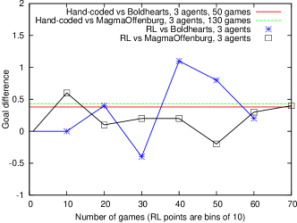
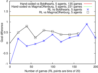
The first experiments were done using a team size of five with the RL agents against Boldhearts. After 140 games our RL agent increased the chance to win from 30% to 50%. This number does not increase more in the next games, but after 260 games the number of lost games (initially  35%) is reduced to 15%. In the further experiments we used the goal difference to compare the performance of the RL agent. Figure (3) shows the average goal differences that the hand-tuned role assignment and the RL agents archive in games against Boldhearts and MagmaOffenburg using different team sizes. With only three agents per team the RL agent only needs 40 games to learn a policy that outperforms the hand-coded role selection (Figure (3(a))). Also with five agents per team, the learning agent is able to increase the goal difference against both opponents (Figure (3(b))). However, it does not reach the performance of the manually tuned role selection. Nevertheless considering the amount of time spent for fine-tuning the hand-coded role selection, these results are promising. Furthermore, the outcome of the games depends a lot on the underlying skills of the agents, such as walking or dribbling. These skills are noisy, thus the results need to be averaged over many games (std. deviations in Figure (3) are between 0.5 and 1.3).

((a)) Three vs three agents.

((b)) Five vs five agents.

((c)) Seven vs seven agents.

Figure 3: Goal difference in games with (a) three; (b) five; and (c) seven agents per team using Greedy-GQ($\lambda$) algorithm.

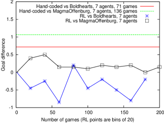
The results in Figure (3(c)) show a bigger gap between RL and the hand-coded agent. However, using seven agents the goal difference is generally decreased, since the defense is easily improved by increasing the number of agents. Also the hand-coded role selection results in a smaller goal difference. Furthermore, considering seven agents in each team the state space is already increased significantly. Only 200 games seem to be not sufficient to learn a good policy. Sometimes the RL agents reach a positive goal difference, but it stays below the hand-coded role selection. In Section 7, we discuss some of the reasons for this inferior performances for the team size seven. Even though the RL agent did not perform well considering only the goal difference, it has learned a moderately satisfactory policy. After 180 games the amount of games won is increased slightly from initially 10% to approximately 20%.

6.2 GVFs with Off-PAC

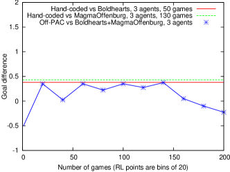
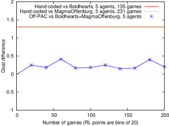
With Off-PAC, we used a similar environment to that of Subsection (6.1), but with a different learning setup. Instead of learning individual policies for teams separately, we learned a single policy for both teams. We ran the opponent teams in a round robin fashion for 200 games and repeated complete runs for multiple times. The first experiments were done using a team size of three with RL agents against both teams. Figure (4(a)) shows the results of bins of 20 games averaged between two trials. After 20 games, the RL agents have learned a stable policy compared to the hand-tuned policy, but the learned policy bounded above the hand-tuned role assignment function. The second experiments were done using a team size of five with the RL agents against opponent teams. Figure (4(b)) shows the results of bins of 20 games averaged among three trials. After 100 games, our RL agent increased the chance of winning to 50%. This number does not increase more in the next games. As Figures (4(a)) and (4(b)) show, the three and five agents per team are able to increase the goal difference against both opponents. However, it does not reach the performance of the manually tuned role selection. Similar to Subsection (6.1), the amount of time spent for fine-tuning the hand-coded role selection, these results are promising, and the outcome of the experiment heavily depends on the underlying skills of the agents.

((a)) Three vs three agents.

((b)) Five vs five agents.

((c)) Seven vs seven agents.

Figure 4: Goal difference in games with (a) three; (b) five; and (c) seven agents per team using Off-PAC algorithm.

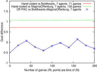
The final experiments were done using a team size of seven with the RL agents against opponent teams. Figure (4(c)) shows the results of bins of 20 games averaged among two trials. Similar to Subsection (6.1), with seven agents per team, the results in Figure (4(c)) show a bigger gap between RL and the hand-tuned agent. However, using seven agents the goal difference is generally decreased, since the defense is easily improved by increasing the number of agents. Also the hand-tuned role selection results in a smaller goal difference. Figure 4(c) shows an increase in the trend of winning games. As mentioned earlier, only 200 games seem to be not sufficient to learn a good policy. Even though the RL agents reach a positive goal difference, but it stays below the hand-tuned role selection method. Within the given setting, the RL agents have learned a moderately satisfactory policy. Whether the learned policy is satisfactory for other teams needs to be further investigated.

The RoboCup 3D soccer simulation is inherently a dynamic, and a stochastic environment. There is an infinitesimal chance that a given situation (state) may occur for many games. Therefore, it is paramount important that the learning algorithms extract as much information as possible from the training examples. We use the algorithms in the on-line incremental setting, and once the experience is consumed it is discarded. Since, we learned from off-policy experiences, we can save the tuples, $(S_{t},A_{t},S_{t+1},r(S_{t+1}),\rho_{t},z(S_{t+1}))$, and learn the policy off-line. The Greedy-GQ($\lambda$) learns a deterministic greedy policy. This may not be suitable for complex and dynamic environments such as the RoboCup 3D soccer simulation environment. The Off-PAC algorithm is designed for stochastic environment. The experiment shows that this algorithm needs careful tuning of learning rates and feature selection, as evident from Figure (4(a)) after 160 games.

7 Conclusions

We have designed and experimented RL agents that learn to assign roles in order to maximize expected future rewards. All the agents in the team ask the question “What is my role in this formation in order to maximize future rewards, while maintaining a completely different role from all teammates in all time steps?”. This is a goal-oriented question. We use Greedy-GQ($\lambda$) and Off-PAC to learn experientially grounded knowledge encoded in GVFs. Dynamic role assignment function is abstracted from all other low-level components such as walking engine, obstacle avoidance, object tracking etc. If the role assignment function selects a passive role and assigns a target location, the lower-layers handle this request. If the lower-layers fail to comply to this request, for example being reactive, this feedback is not provided to the role assignment function. If this information needs to be included; it should become a part of the state representation, and the reward signal should be modified accordingly. The target positions for passive roles are created w.r.t. the absolute ball location and the rules imposed by the 3D soccer simulation league. When the ball moves relatively quickly, the target locations change more quickly. We have given positive rewards only for the forward ball movements. In order to reinforce more agents within an area close to the ball, we need to provide appropriate rewards. These are part of reward shaping [12]. Reward shaping should be handled carefully as the agents may learn sub-optimal policies not contributing to the overall goal.

The experimental evidences show that agents are learning competitive role assignment functions for defending and attacking. We have to emphasize that the behavior policy is $\epsilon$-greedy with a relatively small exploration or slightly perturbed around the target policy. It is not a uniformly distributed policy as used in [22]. The main reason for this decision is that when an adversary is present with the intention of maximizing its objectives, practically the learning agent may have to run for a long period to observe positive samples. Therefore, we have used the off-policy Greedy-GQ($\lambda$) and Off-PAC algorithms for learning goal-oriented GVFs within on-policy control setting. Our hypothesis is that with the improvements of the functionalities of lower-layers, the role assignment function would find better policies for the given question and answer functions. Our next step is to let the RL agent learn policies against other RoboCup 3D soccer simulation league teams. Beside the role assignment, we also contributed with testing off-policy learning in high-dimensional state spaces in a competitive adversarial environment. We have conducted experiments with three, five, and seven agents per team. The full game consists of eleven agents. The next step is to extend learning to consider all agents, and to include methods that select informative state variables and features.

References

- [1] Degris, T., Modayily, J.: Scaling-up Knowledge for a Cognizant Robot. In Notes of the AAAI Spring Symposium on Designing Intelligent Robots: Reintegrating AI (2012)
- [2] Gabel, T., Lange, S., Lauer, M., Riedmiller, M.: Bridging the Gap: Learning in the Robocup Simulation and Midsize League. In: Proceedings of the 7th Portuguese Conference on Automatic Control (Controlo) (2006)
- [3] Gurzoni, Jr., J.A., Tonidandel, F., Bianchi, R.A.C.: Market-Based Dynamic Task Allocation using Heuristically Accelerated Reinforcement Learning. In: Proceedings of the 15th Portugese Conference on Progress in Artificial Intelligence. pp. 365–376. EPIA’11, Springer-Verlag, Berlin, Heidelberg (2011)
- [4] Kober, J., Bagnell, J.A.D., Peters, J.: Reinforcement Learning in Robotics: A Survey. International Journal of Robotics Research (July 2013)
- [5] Köse, H., Tatladede, U., Mericli, C., Kaplan, K., Akan, H.L.: Q-Learning Based Market-Driven Multi-Agent Collaboration in Robot Soccer. In: Proceedings of the Turkish Symposium on Artificial Intelligence and Neural Networks (TAINN). pp. 219–228 (2004)
- [6] MacAlpine, P., Urieli, D., Barrett, S., Kalyanakrishnan, S., Barrera, F., Lopez-Mobilia, A., Ştiurcă, N., Vu, V., Stone, P.: UT Austin Villa 2011: A Champion Agent in the RoboCup 3D Soccer Simulation Competition. In: Proceedings of 11th International Conference on Autonomous Agents and Multiagent Systems (AAMAS 2012) (June 2012)
- [7] Maei, H.R.: Gradient Temporal-Difference Learning Algorithms. PhD Thesis, University of Alberta. (2011), phD Thesis
- [8] Maei, H.R., Sutton, R.S.: GQ(): A General Gradient Algorithm for Temporal-Difference Prediction Learning with Eligibility Traces. Proceedings of the 3rd Conference on Artificial General Intelligence (AGI-10) pp. 1–6 (2010)
- [9] Maei, H.R., Szepesvári, C., Bhatnagar, S., Sutton, R.S.: Toward Off-Policy Learning Control with Function Approximation. In: Proceedings of the 27th International Conference on Machine Learning (ICML 2010). pp. 719–726 (2010)
- [10] Modayil, J., White, A., Pilarski, P.M., Sutton, R.S.: Acquiring a Broad Range of Empirical Knowledge in Real Time by Temporal-Difference Learning. In: Proceedings of the IEEE International Conference on Systems, Man, and Cybernetics (SMC). pp. 1903–1910. IEEE (2012)
- [11] Modayil, J., White, A., Sutton, R.S.: Multi-timescale Nexting in a Reinforcement Learning Robot. In: From Animals to Animats 12 - 12th International Conference on Simulation of Adaptive Behavior (SAB). pp. 299–309 (2012)
- [12] Ng, A.Y., Harada, D., Russell, S.J.: Policy Invariance Under Reward Transformations: Theory and Application to Reward Shaping. In: Proceedings of the Sixteenth International Conference on Machine Learning (ICML). pp. 278–287. Morgan Kaufmann Publishers Inc., San Francisco, CA, USA (1999)
- [13] Pilarski, P., Dawson, M., Degris, T., Carey, J., Sutton, R.: Dynamic Switching and Real-Time Machine Learning for Improved Human Control of Assistive Biomedical Robots. In: 4th IEEE RAS EMBS International Conference on Biomedical Robotics and Biomechatronics (BioRob). pp. 296 –302 (June 2012)
- [14] Riedmiller, M., Gabel, T.: On Experiences in a Complex and Competitive Gaming Domain: Reinforcement Learning Meets RoboCup. In: Third IEEE Symposium on Computational Intelligence and Games. pp. 17–23. IEEE (2007)
- [15] Riedmiller, M., Gabel, T., Hafner, R., Lange, S.: Reinforcement Learning for Robot Soccer. Autonomous Robots 27, 55–73 (July 2009)
- [16] Seekircher, A., Abeyruwan, S., Visser, U.: Accurate Ball Tracking with Extended Kalman Filters as a Prerequisite for a High-Level Behavior with Reinforcement Learning. In: The 6th Workshop on Humanoid Soccer Robots at Humanoid Conference, Bled (Slovenia) (2011)
- [17] Stoecker, J., Visser, U.: Roboviz: Programmable Visualization for Simulated Soccer. In: Röfer, T., Mayer, N.M., Savage, J., Saranli, U. (eds.) RoboCup. pp. 282–293. Lecture Notes in Computer Science, Springer (2011)
- [18] Stone, P., Sutton, R.S., Kuhlmann, G.: Reinforcement Learning for RoboCup-Soccer Keepaway. Adaptive Behavior 13(3), 165–188 (2005)
- [19] Stone, P., Veloso, M.: Layered Learning. In: Proceedings of the Eleventh European Conference on Machine Learning. pp. 369–381. Springer Verlag (1999)
- [20] Stone, P., Veloso, M.: Task Decomposition, Dynamic Role Assignment, and Low-Bandwidth Communication for Real-Time Strategic Teamwork. Artificial Intelligence 110(2), 241–273 (June 1999)
- [21] Sutton, R.S., Barto, A.G.: Reinforcement Learning: An Introduction. MIT Press (1998)
- [22] Sutton, R.S., Modayil, J., Delp, M., Degris, T., Pilarski, P.M., White, A., Precup, D.: Horde: A Scalable Real-Time Architecture for Learning Knowledge from Unsupervised Sensorimotor Interaction. In: The 10th International Conference on Autonomous Agents and Multiagent Systems. pp. 761–768. AAMAS ’11, International Foundation for Autonomous Agents and Multiagent Systems (2011)
- [23] Sutton, R.S., Szepesvári, C., Maei, H.R.: A Convergent O(N) Algorithm for Off-Policy Temporal-Difference Learning with Linear Function Approximation. In: Advances in Neural Information Processing Systems (NIPS). pp. 1609–1616. MIT Press (2008)
- [24] Thomas Degris, Martha White, R.S.S.: Off-Policy Actor-Critic. In: Proceedings of the Twenty-Ninth International Conference on Machine Learning (ICML) (2012)
- [25] White, A., Modayil, J., Sutton, R.: Scaling Life-Long Off-Policy Learning. In: International Conference on Development and Learning and Epigenetic Robotics (ICDL), 2012 IEEE. pp. 1–6 (2012)