Central elements in the universal enveloping algebra and function of matrix elements.

In the paper a construction of central elements in $U(\mathfrak{o}_{N})$ and $U(\mathfrak{g}_{2})$ based on invariant theory is given. New function of matrix elements that appear in description of the center of $U(\mathfrak{g}_{2})$ are defined.

1 Introduction

Let $\mathfrak{g}$ be a simple Lie algebra and let $V$ be it’s standard representation, put $dimV=N$. Central elements in the universal enveloping algebra $U(\mathfrak{g})$ can be expressed as functions of matrix elements of the matrix $L$ that is defined below, for different algebras different functions (determinants, pfaffians, hafnians) are used [1], [2], [6]. However in cited papers the mentioned functions of matrix elements are not derived from some required properties. The corresponding formulas are presented and then it is proved that define central elements.

In the present paper a general construction of central elements is given. In the case of orthogonal algebra it leads to formulas involving pfaffians. Also this scheme is applied to the exceptional algebra $\mathfrak{g}_{2}$, in this case we obtain some new functions of matrix elements.

Let us define the matrix $L$. Let $v_{\alpha}$ be a base in $\mathfrak{g}$, and $V_{\alpha}$ be a matrix that correspond to $v_{\alpha}$ in the standard representation. Put

$$L=V_{\alpha}\otimes v_{\alpha}.$$

Note that $L$ can be considered as an $N\times N$ matrix, whose elements belong to $\mathfrak{g}$. Then the following facts take place

1. In the case when $\mathfrak{g}$ belongs to the series $A$, in $U(\mathfrak{g})$ there are central elements given by the formula

   $$C_{k}=\sum_{|I|=k}DetL_{I},\,\,\,\,k=2,...,N$$ (1)

   where $I\subset\{1,...,N\}$, and $L_{I}$ is a submatrix in $L$, defined as $L_{I}=(L_{ij})_{i,j\in I}$, and $Det$ is a double determinant (see formula (2)). The summation is taken over all subsets $I\subset\{1,...,N\}$ that consist of $k$ elements.

   In particular the element

   $$\begin{split}Det(L)=\frac{1}{N!}\sum_{\sigma,\sigma^{\prime}\in S_{N}}L_{\sigma(1),\sigma^{\prime}(1)}...L_{\sigma(N),\sigma^{\prime}(N)}\end{split}$$ (2)

   is central.

2. In the case when $\mathfrak{g}$ belongs to the series $B$ or $D$, in $U(\mathfrak{g})$ there are the following matrix elements

   $$C_{2}k=\sum_{|I|=k}(PfL_{I})^{2},\,\,\,\,$$ (3)

   where $k=1,...,N/2$ in the case of series $D$ and $k=1,...,(N-1)/2$ in the case of series $B$.

   Also in the case $D$ the element

   $$\begin{split}PfL=\frac{1}{N!2^{N}}\sum_{\sigma\in S_{2N}}L_{\sigma(1),\sigma(2)}...L_{\sigma(2N-1),\sigma(2N)}\end{split}$$ (4)

   is central.

3. In the case when $\mathfrak{g}$ belongs to the series $C$ in the universal enveloping algebra there are central elements that are expressed through the so called hafnians of submatrices of the matrix $L$ [6].

Thus one can say that in the case of the series $A$ the central elements are expressed through determinants, in the case of the series $B$, $D$ the central elements are expressed through pfaffians. But for exceptional Lie algebras a relation between central elements and new functions of matrix elements is not pointed out.

There appears a question. Why in construction of central elements in the case of series $B$, $D$ the pfaffians and not other function of matrix elements appear? Which functions appear in the construction of central elements in the case of the algebra $\mathfrak{g}_{2}$?

2 The content of the paper

In the present paper a construction of central elements in the universal enveloping algebra based on the first main theorem of the invariant theory is given. For the construction of the central elements a notion of an $m$-invariant is introduced. An $m$-invariant is polynomial in variables $m_{i,j}$, $i,j\in\{1,...,N\}$, that is invariant under the action of the Lie algebra $\mathfrak{g}$. The action of the generator $v$ of the Lie algebra, to which in the standard representation there corresponds the matrix $V$, on these variables is given by formula

$$m_{i,j}\mapsto V_{i,c}m_{c,j}+m_{i,d}V_{j,d}.$$

It is proved in the present paper that in the case of series $A$, $B$, $C$, $D$, and also in the case $\mathfrak{g}_{2}$ when one substitute into an $m$-invariant elements $L_{i,j}$ instead of $m_{i,j}$, and $L_{i,j}$ are multiplied using the symmetrized product, one gets a central element in $U(\mathfrak{g})$.

In Section 5 the cases of series $B$ and $D$ are considered. Using the first main theorem of the invariant theory a description of a general $m$-invariant is given. Then we present new relations that appear when one substitutes $L_{i,j}$ instead of $m_{i,j}$. As a corollary one obtains a well known description of the center of $U(\mathfrak{o}_{N})$. Let us stress that in this approach the pfaffians in formulas appear very natural from the first main theorem of the invariant theory.

Secondly in Section 6 the case of the exceptional Lie algebra $\mathfrak{g}_{2}$ is considered. The central elements for $\mathfrak{g}_{2}$ are constructed using the first main theorem of the invariant theory.

In Section 6.4 we define some new functions of matrix elements through which the central elements are expressed. Let us write some of these functions. Let $M=(m_{ij})$ be a $8\times 8$ matrix(or $7\times 7$ matrix), whose rows and columns are indexed by octonions (imaginary octonions). Let $\omega_{i_{1},i_{2},i_{3}}$ be structure constants of octonions. Put

$$\omega_{i_{1},...,i_{k}}:=skew_{i_{1},...,i_{k}}\omega_{i_{1},i_{2},s_{1}}\omega_{s_{1},i_{3},s_{2}}...\omega_{s_{k-1},i_{k},1},$$ (5)

where $skew_{i_{1},...,i_{k}}$ denotes antisymmetrization of the indices $i_{1},...,i_{k}$. This tensor is skewsymmetric. Then the new function of matrix elements are

$$\begin{split}G_{k}^{k}(L)=\omega_{i_{1},...,i_{k}}\omega_{j_{1},...,j_{k}}m_{i_{1},j_{1}}...m_{i_{k},j_{k}}\end{split}$$ (6)

Also in Section 6.4 other functions appear.

However when one substitutes $L_{i,j}$ instead of $m_{i,j}$ into these functions during the construction of central elements it turns out to be possible to express functions (6) through determinants of submatrices of the matrix $L$.

3 Preliminaries

3.1 Invariant polynomials. The first main theorem of the invariant theory. $m$-invariants.

Let us be given a Lie algebra $\mathfrak{g}$, let $V$ be it’s standard representation. Let $x_{1},...,x_{m}$ be vectors from $V$, put $dimV=N$, and denote as $x_{k}^{i}$, $i=1,...,N$ the coordinates of vectors $x_{k}$.

The first main theorem of the invariant theory is a theorem that describes generators in the algebra of polynomials in variables $x_{k}^{i}$, that are invariant under the action of $\mathfrak{g}$.

We call an invariant polynomial in variables $x_{k}^{i}$ an $x$-invariant.

Let us be given an $N\times N$ matrix $M$, whose elements are variables $m_{ij}$ with no relations between them. Define an action on the variables $m_{ij}$ of the element $v$ algebra $\mathfrak{g}$ by formulas

$$M\mapsto VM+MV^{t},\text{ or }m_{ij}\mapsto V_{ik}m_{kj}+m_{jl}V_{il},$$ (7)

where $v\in\mathfrak{g}$, and $V_{i,j}$ is a matrix, corresponding to $v$ in the standard representation.

Definition 1.

A polynomial $m_{ij}$, that is invariant under the action of the algebra is called an $m$-invariant.

There exist an obvious correspondence between homogeneous $x$-invariant of degree $2k$ and homogeneous $m$-invariant of degree $k$. To an $x$-invariant

$$t^{i_{1},j_{1}...,i_{k},j_{k}}x^{1}_{i_{1}}x^{1^{\prime}}_{i^{\prime}_{1}}...x^{k}_{i_{k}}x^{k^{\prime}}_{i^{\prime}_{k}}$$

there corresponds an $m$-invariant

$$t^{i_{1},j_{1}...,i_{k},j_{k}}m_{i_{1},j_{1}}...m_{i_{k}j_{k}}.$$

4 A relation between $m$-invariants and central elements in the universal enveloping algebra

Let us for an algebra $\mathfrak{g}$ construct a matrix $L$ whose elements belong to $\mathfrak{g}$. Let $v_{\alpha}$ be a base in $\mathfrak{g}$ and denote as $V_{\alpha}$ a matrix corresponding to $v_{\alpha}$ in the standard representation. Put

$$L=V_{\alpha}\otimes v_{\alpha}.$$

In the case $\mathfrak{g}=\mathfrak{o}_{N}$ the matrix $L$ up to multiplication by a constant equals to

$$(F_{i,j}),\,\,\,i,j=1,...,N,$$

where generators $F_{i,j}$ are defined by formula $F_{i,j}=E_{i,j}-E_{j,i}.$ Thus the matrix $L$ is skew-symmetric.

In the case $\mathfrak{g}=\mathfrak{g}_{2}$ the matrix $L$ up to multiplication by a constant equals to

$$(G_{i,j}),\,\,\,i,j=1,...,7,$$

where generators $G_{i,j}$ are defined as follows. The Lie algebra $\mathfrak{g}_{2}$ is the algebra of differentiations of octonions. For octonions $x,y$ define a differentiation $G_{x,y}$ that act on an octonion $z$ as follows

$$G_{x,y}(z)=[[x,y],z]-3[x,y,z]\text{ where }[x,y,z]=(xy)z-x(yz).$$

Take a standard base $1,e_{1},...,e_{7}$ in the algebra of octonions, such that $e_{1},...,e_{7}$ are standard imaginary octonions, take $x=e_{i},y=e_{j}$ and put

$$G_{i,j}=G_{e_{i},e_{j}}.$$

In the case of both algebras $\mathfrak{o}_{N}$ and $\mathfrak{g}_{2}$ commutation relations between generators can be written in a similar way. For $g\in\mathfrak{o}_{N}$ define the element $F_{g\{i_{1},i_{2}\}}$ as follows. Identify a pair of indices $\{i_{1},i_{2}\}$ with the wedge-product of vectors of standard representation $e_{i_{1}}\wedge e_{i_{2}}$. Let

$$g(e_{i_{1}}\wedge e_{i_{2}})=c_{\alpha}e_{p_{\alpha}}\wedge e_{q_{\alpha}}.$$

Then put

$$F_{g\{i_{1},i_{2}\}}=c_{\alpha}F_{p_{\alpha},q_{\alpha}}.$$

In [3] it is shown that commutation relations between generators of $\mathfrak{o}_{N}$ can be written as follows

$$[g,F_{i,j}]=F_{g\{i,j\}},\,\,\,g\in\mathfrak{o}_{N}$$ (8)

Analogously in [5] it is shown that in the case $\mathfrak{g}_{2}$ one has

$$[g,G_{i,j}]=G_{g\{i,j\}},\,\,\,g\in\mathfrak{g}_{2}.$$ (9)

Below we denote as $L_{i,j}$ the generators $F_{i,j}$ in the case $\mathfrak{o}_{N}$ and generators $G_{i,j}$ in the case $\mathfrak{g}_{2}$.

Let us prove Proposition.

Proposition 1.

In the case of algebras $\mathfrak{g}=\mathfrak{o}_{N}$, $\mathfrak{g}_{2}$ if

$$T=t^{i_{1},j_{1}...,i_{k},j_{k}}m_{i_{1},j_{1}}...m_{i_{k}j_{k}}$$

is an $m$-invariant, then

$$\overline{T}=t^{i_{1},j_{1}...,i_{k},j_{k}}L_{i_{1},j_{1}}\cdot...\cdot L_{i_{k}j_{k}}$$

is a central element in $U(\mathfrak{g})$. Here $\cdot$ is a symmetrized product.

Proof.

There exist a mapping

$$m_{ij}\mapsto L_{ij}$$ (10)

from the algebra of polynomials in variables $m_{ij}$ into the algebra of polynomials in variables $L_{ij}$ with the symmetrized product. The last algebra is embedded in $U(\mathfrak{g})$.

According to formulas (8), (9) the mapping given by the formula (10), transforms the action of an element $g\in\mathfrak{g}$ on the polynomials $m_{ij}$ into the operation of commutation $[g,.]$. Hence the invariant polynomials are mapped into central elements.

∎

5 Orthogonal algebra

In the Section the first main theorem of the invariant theory is formulated. Using this theorem generators in the algebra of $m$-invariants are written. These generators are encoded by graphs. Relations between these generators are written. These relations allow to define basic $m$-invariants and to express all invariant though basic invariants.

5.1 The first main theorem

Theorem 1.

(see [4]) Let $x_{1},...,x_{m}$be vectors of the standard representation $V$ of the algebra $\mathfrak{o}_{N}$. Then the algebra of polynomials in coordinates of vectors $x_{k}$ that are invariant under the action of $\mathfrak{o}_{N}$ is generated by $(x_{k},x_{l})=\sum_{i}x_{k}^{i}x_{l}^{i}$ for all $k,l$, and also in the case $N=m$, by the polynomial $det(x_{k}^{i})=det[x_{1},...,x_{N}]$, where $[x_{1},...,x_{N}]$ is a matrix that is constructed from the columns of coordinates of vectors $x_{1},...,x_{N}$.

5.2 Examples of $m$-invariants.

Using the correspondence between $x$ and $m$-invariants let us construct examples of $m$-invariants.

5.2.1 The trace

Take as an $x$-invariant the scalar product. That is put $T(x_{1},x_{2})=x_{1}^{i}x_{2}^{i}$. Then the corresponding $m$-invariant is the trace of $M$.

5.2.2 The pfaffian

Take as an $x$-invariant the determinant. That is $T(x_{1},...,x_{k})=det[x^{1},...,x^{k}]$. The components of $T$ are the following

$$t^{i_{1},j_{1}...,i_{k},j_{k}}=0,\text{ if }\{i_{1},j_{1}...,i_{k},j_{k}\}\neq\{1,...,2k\},$$

$$t^{i_{1},j_{1}...,i_{k},j_{k}}=(-1)^{\sigma},\text{ if }(i_{1},j_{1}...,i_{k},j_{k})=(\sigma(1),...,\sigma(2k)).$$

The corresponding $m$-invariant equals

$$k!2^{k}PfM.$$

5.2.3 The determinant

Take the following $x$-invariant

$$T(x_{1},x_{1^{\prime}},...,x_{k},x_{k^{\prime}})=det[x_{1},...,x_{k}]det[x_{1^{\prime}}...x_{k^{\prime}}].$$

In the components one gets

$$t^{i_{1},j_{1}...,i_{k},j_{k}}=0,\text{ if }\{i_{1},...,i_{k},\}\neq\{1,...,k\},\text{ or }\{j_{1},...,j_{k},\}\neq\{1,...,k\}$$

$$t^{i_{1},j_{1}...,i_{k},j_{k}}=(-1)^{\sigma}(-1)^{\sigma^{\prime}},\text{ if }(i_{1},...,i_{k})=(\sigma(1),...,\sigma(2)),\,\,\,\,(j_{1}...,j_{k})=(\sigma^{\prime}(1),...,\sigma^{\prime}(2k))$$

The corresponding $m$-invariant equals

$$k!detM.$$

5.3 The graphical description of $m$-invariants

Let us describe a general $m$-invariant. The general $x$-invariant is a linear combination of traces and determinants. Let us find an $m$-invariant that correspond to such $x$-invariant.

A general $m$-invariant is encoded by an oriented graph with some additional information of the following kind. The vertices are of colored into two colors: white or black. Every black vertex belongs to exactly $n$ edges the number $n$ is the same for all edges. An order on the edges that belong to a black vertex is fixed. A white vertex belongs to two edges. All edges are numerated by numbers from $1$ to $K$.

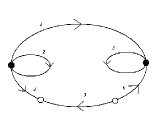
Figure 1: A graph that encodes an $m$-invariant

To construct an $m$-invariant we take the product $m_{i_{1},j_{1}}...m_{i_{K},j_{K}}$.

To every white vertex there corresponds a contraction.

In the case when the edges with numbers $a$, $b$ begin in this vertex one takes the contraction

$$m_{i_{a},c}m_{i_{b},c}.$$

In the case when the edges with numbers $a$, $b$ end in this vertex one takes the contraction

$$m_{c,j_{a}}m_{c,j_{b}}.$$

In the case when the edge $a$ ends in the considered vertex and the edge with the number $b$ begins in the vertex one takes the contraction (see figure 2)

$$m_{i_{a},c}m_{c,j_{b}}.$$

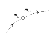
Figure 2: A contraction corresponding to a white vertex

To every black vertex there corresponds an antisymmetrization. Suggest that the black vertex belongs to edges with numbers $a_{1}$,…,$a_{n}$. For every edge with the number $a_{k}$ take the index $i_{a_{k}}$ if the edge begins in the vertex and take the index $b_{k}$ if the edge ends in the vertex. Then an antisymmetrization of the chosen indices is taken. The obtained expression is an $m$-invariant, that corresponds to a graph.

This description of $m$-invariants follows from the description of $x$-invariant and the construction of $m$-invariant from $m$-invariants.

Remark 2.

An $m$-invariant can be written as a linear combination of products of determinants and pfaffians of submatrices of products of $M$ and $M^{t}$. However this description is needed below.

Let us describe graphs that correspond to invariants from the subsection 5.2.

To the trace there corresponds the graph shown in the figure 3.

Figure 3: A graph that encodes a trace

To the pfaffian in the case $k=2$ there corresponds the graph from the figure 4

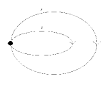
Figure 4: A graph that encodes a pfaffian

To the determinant in the case $k=2$ there corresponds a graph shown in the figure 5

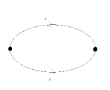
Figure 5: A graph that encodes a determinant

5.4 Relations

If one puts no relation on the matrix $M=(m_{ij})$ then all relations between $m$-invariants are corollaries of relations between $x$-invariant, these relation are well-known (see the second main theorem in the invariant theory in [4]).

For the element of the matrix $L$ there exist the following relation of skew-symmetry

$$L_{i,j}=-L_{j,i}.$$

Let us put onto the elements $M$ relations of skew symmetry $m_{i,j}=-m_{j,i}$. In this case in addition to relations following from the second main theorem of the invariant theory new relations between $m$-invariants appear. These relation allow to define basic invariants and to express other invariant though them.

Let us as formulate these relation.

5.4.1 The first relation

In the case of skew symmetric matrix $M$ of size $2\times 2$ the following obvious relation takes place

$$(PfM)^{2}=DetM.$$

It gives a relation shown in the figure 6. This figure states the following relation. Let us be given a graph where from one black vertex to another one go two similar paths though white vertices (in these paths the same are the numbers of white vertices and orientations of edges). Then the corresponding $m$-invariant equals to an $m$-invariant that is defined by the graph where these paths go not from one black vertex to another but from return to the same black vertex.

Figure 6: The first relation

5.4.2 The second relation

In the case of matrices $M$ and $M^{\prime}$ of size $2\times 2$ one has

$$\begin{split}&Det(M+M^{\prime})-DetM-DetM^{\prime}=\frac{1}{2}(m_{1,1}m^{\prime}_{2,2}-m_{2,1}m^{\prime}_{1,2}-m_{1,2}m^{\prime}_{2,1}+m_{2,2}m^{\prime}_{1,1}+\\ &+m^{\prime}_{2,2}m_{1,1}-m^{\prime}_{1,2}m_{2,1}-m^{\prime}_{2,1}m_{1,2}+m^{\prime}_{1,1}m_{2,2})\end{split}$$ (11)

This equality gives a relation shown on the picture 7. On this picture the first graph on the right side of the equality denotes the following invariant. First one takes a $2\times 2$-matrix that corresponds to the path with $n$ white vertices. Then one takes as analogous product for the path with $m$ white vertices. Then one takes a sum of these matrices and then one takes it’s determinant.

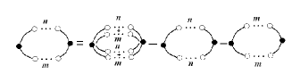
Figure 7: The second relation

5.4.3 The third relation

In the case of skew-symmetric matrices $M$ and $M^{\prime}$ of size $4\times 4$ one has an equality

$$\begin{split}&Pf(M+M^{\prime})-PfM-PfM^{\prime}=\frac{1}{2}(m_{1,2}m^{\prime}_{3,4}-m_{1,3}m^{\prime}_{2,4}+m_{1,4}m^{\prime}_{2,3}+\\ &+m^{\prime}_{3,4}m_{1,2}-m^{\prime}_{2,4}m_{1,3}+m^{\prime}_{2,3}m_{1,4})\end{split}$$ (12)

This equality gives us a relation shown in the figure 8.

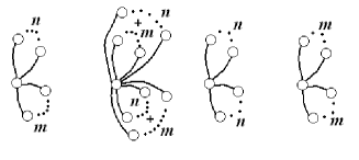
Figure 8: The third relation

5.4.4 The fourth relation

In the case of skew symmetric matrix $M$ one has a relation

$$Pf(M^{k})=(PfM)^{k}.$$

5.4.5 Basic invariants

Using the relations above in the case of skew-symmetric matrix $M$ one can express every relation through the $m$-invariant of type

$$Tr(M^{k})\text{ or }Pf(M^{n_{1}}+...+M^{n_{k}}).$$ (13)

Using standard formulas connecting different symmetric polynomials one can express the invariants (13) through the invariants

$$\sum_{|I|=k}(PfM_{I})^{2},\text{ or }PfM\,\,\,\,I\subset\{1,...,N\},\,\,\,M_{I}=(m_{i,j})_{i,j\in I}.$$ (14)

6 The algebra $\mathfrak{g}_{2}$

Let us formulate the first main theorem of the invariant theory in the case of the algebra $\mathfrak{g}_{2}$. Using this theorem let us describe $m$-invariants and central elements. Some of these central elements are written explicitly.

6.1 The first main theorem of the invariant theory

Theorem 2.

(see [7],[8]) Let $x_{1},...,x_{m}$ be vectors of the standard representation $V$ of the algebra $\mathfrak{g}_{2}$. Then the algebra of invariant polynomials in variables $x_{1},...,x_{m}$ is generated by polynomials

$$str(x_{j_{1}}(x_{j_{2}}(x_{j_{3}}...x_{j_{r}})...))),$$

where vectors are multiplied as octonions and $str$ denotes the symmetrized trace. And the trace denotes the operation of taking the real part.

Let us give another formulation of this theorem. Denote as $\omega_{i_{1},i_{2},i_{3}}$ the structure constants of octonions. Put

$$\omega_{i_{1},...,i_{k}}:=skew\omega_{i_{1},...,i_{k}}\omega_{i_{1},i_{2},s_{1}}\omega_{s_{1},i_{3},s_{2}}...\omega_{s_{k-1},i_{k},1},$$ (15)

where $skew_{i_{1},...,i_{k}}$ denotes antisymmetrization of the indices $i_{1},...,i_{k}$.

One describe this tensor as follows. Identify the index $i_{s}$ with the basic octionon $e_{i_{s}}$, then $\omega_{i_{1},...,i_{k}}$ is a skew-symmetric $k$-tensor, it’s component equals to $0$, if

$$e_{i_{1}}....e_{i_{k}}\neq\pm 1,$$

its component equals to $1$, if

$$e_{i_{1}}....e_{i_{k}}=1.$$

Using this tensor one can reformulate the first main theorem as follows

Theorem 3.

Let $x_{1},...,x_{m}$ be vectors of the standard representation $V$ of the algebra $\mathfrak{g}_{2}$. Then the algebra of polynomials in coordinates of vectors $x_{1},...,x_{m}$ is generated by polynomials

$$\omega_{i_{1},...,i_{k}}x_{j_{1}}^{i_{1}}....x_{j_{k}}^{i_{k}}.$$

6.2 $m$-invariant

Let us give description of $m$-invariants, using the first main theorem of the invariant theory.

Consider a product

$$m_{i_{1},j_{1}}...m_{i_{k},j_{k}}.$$

Let us divide the set of indices $\{i_{1},j_{1},...,i_{k},j_{k}\}$ into $p$ groups $\{a_{1},...,a_{s}\}$,…,$\{b_{1},...,b_{t}\}$. The indices of the first group are contracted with $\omega_{a_{1},...,a_{s}}$,…, the indices in the last group are contracted with $\omega_{b_{1},...,b_{t}}$.

One can give a graphical description of an $m$-invariant. An invariant is described by an oriented graph whose edges are numerated by numbers $1,...,p$. To the edge with the number $l$ there corresponds $m_{i_{l},j_{l}}$. A vertex where the edges with numbers $a_{1},...,a_{s}$ end end the edges with numbers $b_{1},...,b_{t}$ begin there correspond a contraction

$$j_{a_{1}},...,j_{a_{s}},i_{b_{1}},...,i_{b_{t}}\text{ с }\omega_{j_{a_{1}},...,j_{a_{s}},i_{b_{1}},...,i_{b_{t}}}.$$

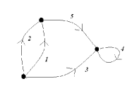
Figure 9: A graph that encodes an $\mathfrak{g}_{2}$-invariant

6.3 Central elements

Let us find, which $m$-invariant give nonzero central elements. In the case of the algebra $\mathfrak{g}_{2}$ the elements $L_{ij}$ satisfy the relation [9]

$$L_{ij}\omega_{i,j,l}=0$$ (16)

Using this relation and the description of $m$-invariants for $\mathfrak{g}_{2}$ from Section 6.2 one finds that the central elements are describes as follows. One takes a product

$$L_{i_{1},j_{1}}...L_{i_{k},j_{k}},$$

then the set of indices $\{i_{1},j_{1}...,i_{k},j_{k}\}$ is divided into subsets $\{a_{1},...,a_{t}\}\sqcup...\sqcup\{b_{1},...,b_{t}\}$, where one set set does not contain $i_{l},j_{l}$ simultaneously. Then every set of indices is contracted with the corresponding tensor $\omega$.

6.4 The functions $G$

Let $M=(m_{ij})$ be a $8\times 8$ (or $7\times 7$) matrix, whose rows and columns are indexed by octonions (imaginary octionos).

Fix an integer $k$, $2\leq k\leq 8$, integers $n_{1},...,n_{p}$, $n_{1}+...+n_{p}=k$ and $m_{1},...,m_{q}$, $m_{1}+...+m_{q}=k$

$$\begin{split}&G_{m_{1},...,m_{q}}^{n_{1},...,n_{p}}(L)=\\ &=\sum_{\{i_{1},...,i_{k}\}=I_{1}\sqcup...\sqcup I_{p},\{j_{1},...,j_{k}\}=J_{1}\sqcup...\sqcup J_{q}}\omega_{i^{1}_{1},...,i^{1}_{n_{1}}}...\omega_{i^{1}_{p},...,i^{p}_{n_{p}}}\omega_{j^{1}_{1},...,j^{1}_{m_{1}}}...\omega_{j^{q}_{1},...,j^{q}_{m_{q}}}L_{i_{1},j_{1}}...L_{i_{k},j_{k}},\end{split}$$ (17)

where the first summation is taken over all partitions of the sets $I=\{i_{1},...,i_{k}\}$ и $J=\{j_{1},...,j_{k}\}$ such that $I_{1}=\{i_{1}^{1},...,i^{1}_{n_{1}}\}$,…,$J_{1}=\{j_{1}^{1},...,j^{1}_{m_{1}}\}$….

As it is proved above the functions $G_{m_{1},...,m_{q}}^{n_{1},...,n_{p}}(L)$ generate the algebra of central elements in $U(\mathfrak{g}_{2})$.

However there exist relations between these generators. Actually when writes the basic central elements the corresponding functions $G_{m_{1},...,m_{q}}^{n_{1},...,n_{p}}(L)$ can be expressed through the determinants and pfaffians.

6.5 Examples

It is known that in $U(\mathfrak{g}_{2})$ the exist primitive central elements of orders $2$ and $6$.

6.5.1 The central element of the order $2$.

Consider the invariant of the order $2$. Is is given by the function $G_{2}^{2}(L)$. To write it let us take the product

$$L_{i_{i},j_{1}}L_{i_{2},j_{2}},$$ (18)

the indices $i_{1},i_{2}$ must be contracted with $\omega_{i_{1},i_{2},1}$, and the indices $j_{1},j_{2}$ must be contracted with $\omega_{j_{1},j_{2},1}$.

Since $\omega_{i_{1},i_{2},i_{3}}$ are structure constants of octonions, and squares of base octonions equal to $-1$, then

$$\omega_{i_{1},i_{2},1}=-1\Leftrightarrow i_{1}=i_{2}.$$

Hence the contraction is actually a sum

$$L_{i_{i},j_{1}}L_{i_{1},j_{1}}.$$ (19)

Thus the central element is the Casimir element.

6.5.2 The central element of higher orders.

Consider the invariant of order $m$ that is defined by the function $G_{m}^{m}(L)$. To write it let us take the product

$$L_{i_{i},j_{1}}...L_{i_{m},j_{m}},$$ (20)

indices $i_{1},...,i_{m}$ are contracted with $\omega_{i_{1},...,i_{m}}$, а indices $j_{1},...,j_{m}$ are contracted with $\omega_{j_{1},...,j_{m}}$.

There exist $7$ imaginary octonions and there product equals $\pm 1$.

the contraction with $\omega_{i_{1},...,i_{6}}$ can be done as follows. Thus one obtains that $\omega_{j_{1},...,j_{m}}=0$ for $m=5,6$, and for $m=7$ the contraction with $\omega_{j_{1},...,j_{7}}$ is just an antisymmetrization over indices $i_{1},...,i_{7}$.

The central elements corresponding to $m=3,4$ can be expressed through the Casimir element (since primitive central elements have orders $2,6$) and the element corresponding to $m=7$ equals to $detL$.

6.6 Conclusion

A construction of central elements in $U(\mathfrak{o}_{N})$ is given. In this construction pfaffians appear in a natural manner.

Also a construction of central elements in $U(\mathfrak{g}_{2})$ is given. In this construction new functions of central elements $G_{m_{1},...,m_{q}}^{n_{1},...,n_{p}}(L)$ given by formula (LABEL:new1) appeared.

References

- [1] R. Howe, T. Umeda, The Capelli identtity, the double commutant theorem and multiplicity-free actions, Math. Ann. 1991, 290, 565-619.
- [2] M. Itoh, T. Umeda. On Central Elements in the Universal Enveloping Algebras of the Orthogonal Lie Algebras, Compositio Mathematica, 2001, 127, 333-359.
- [3] D.V. Artamonov, V.A. Golubeva, Noncommutative Pfaffians associated with the orthogonal algebra, Sbornik Math., 203, 2012, 5-34
- [4] H. Weyl, The classical groups, their invariants and representations, Springer, 1939.
- [5] D.V. Artamonov, V.A. Golubeva, Capelli elements for the Lie algebra , J. Lie Theory, 2013, 23, 589-606
- [6] A. Molev, Yangians and classical Lie algebras, AMS, Mathematical Surveys and Monographs, vol. 143, 2007.
- [7] G. Schwarz, Invariant theory of , Bull. of AMS, v. 8, 1983, 335-388.
- [8] G. Schwarz, Invariant theory of and , Comment. Math. Helvetici, 63, 1988, 624-663.
- [9] L. Frappat, A. Sciarrino, P. Sorba, Dictionary on the Lie algebras and Superalgebras, Academic Press, 2000