11institutetext: Department of Mathematics, University of Geneva, Switzerland. Martin.Gander@unige.ch,Felix.Kwok@unige.ch,Bankim.Mandal@unige.ch

Dirichlet-Neumann and Neumann-Neumann Waveform Relaxation for the Wave Equation

Martin J. Gander 11    Felix Kwok and Bankim C. Mandal 1111

1 Introduction

We present two new types of Waveform Relaxation (WR) methods for hyperbolic problems based on the Dirichlet-Neumann and Neumann-Neumann algorithms, and present convergence results for these methods. The Dirichlet-Neumann algorithm for elliptic problems was first considered by Bjørstad & Widlund BjWid ; the Neumann-Neumann algorithm was introduced by Bourgat et al. BouGT . The performance of these algorithms for elliptic problems is now well understood, see for example the book TosWid .

To solve time-dependent problems in parallel, one can either discretize in time to obtain a sequence of steady problems, and then apply domain decomposition algorithms to solve the steady problems at each time step in parallel, or one can first discretize in space and then apply WR to the large system of ordinary differential equations (ODEs) obtained from the spatial discretization. WR has its roots in the work of Picard and Lindelöf, who studied existence and uniqueness of solutions of ODEs in the late 19th century. Lelarasmee, Ruehli and Sangiovanni-Vincentelli LelRue rediscovered WR as a parallel method for the solution of ODEs. The main computational advantage of WR is parallelization, and the possible use of different discretizations in different space-time subdomains.

Domain decomposition methods for elliptic PDEs can be extended to time-dependent problems by using the same decomposition in space. This leads to WR type methods, see Bjor . The systematic extension of the classical Schwarz method to time-dependent parabolic problems was started independently in GanStu ; GilKel . Like WR algorithms in general, the so-called Schwarz Waveform Relaxation algorithms (SWR) converge relatively slowly, except if the time window size is short. A remedy is to use optimized transmission conditions, which leads to much faster algorithms, see GH1 for parabolic problems, and GHN for hyperbolic problems. More recently, we studied the WR extension of the Dirichlet-Neumann and Neumann-Neumann methods for parabolic problems GKM1 ; Mandal ; Kwok . We proved for the heat equation that on finite time intervals, the Dirichlet-Neumann Waveform Relaxation (DNWR) and the Neumann-Neumann Waveform Relaxation (NNWR) methods converge superlinearly for an optimal choice of the relaxation parameter. DNWR and NNWR also converge faster than classical and optimized SWR in this case.

In this paper, we define DNWR and NNWR for the second order wave equation

$\displaystyle\partial_{tt}u-c^{2}\Delta u$ $\displaystyle=f(\boldsymbol{x},t),$ $\displaystyle\boldsymbol{x}\in\Omega,0<t<T,$
$\displaystyle u(\boldsymbol{x},0)$ $\displaystyle=u_{0}(\boldsymbol{x}),\;u_{t}(\boldsymbol{x},0)=v_{0}(\boldsymbol{x}),$ $\displaystyle\boldsymbol{x}\in\Omega,$ (1)
$\displaystyle u(\boldsymbol{x},t)$ $\displaystyle=g(\boldsymbol{x},t),$ $\displaystyle\boldsymbol{x}\in\partial\Omega,0<t<T,$

where $\Omega\subset\mathbb{R}^{d}$, $d=1,2,3$, is a bounded domain with a smooth boundary, and $c$ denotes the wave speed, and we analyze the convergence of both algorithms for the 1d wave equation.

2 Domain decomposition and algorithms

To explain the new algorithms, we assume for simplicity that the spatial domain $\Omega$ is partitioned into two non-overlapping subdomains $\Omega_{1}$ and $\Omega_{2}$. We denote by $u_{i}$ the restriction of the solution $u$ of (1) to $\Omega_{i}$, $i=1,2$, and by $n_{i}$ the unit outward normal for $\Omega_{i}$ on the interface $\Gamma:=\partial\Omega_{1}\cap\partial\Omega_{2}$.

The Dirichlet-Neumann Waveform Relaxation algorithm (DNWR) consists of the following steps: given an initial guess $h^{0}(x,t)$, $t\in(0,T)$ along the interface $\Gamma\times(0,T)$, compute for $k=1,2,...$ with $u_{1}^{k}=g,$ on $\partial\Omega_{1}\setminus\Gamma$ and $u_{2}^{k}=g,$ on $\partial\Omega_{2}\setminus\Gamma$ the approximations

$$\begin{array}[]{c}\begin{array}[]{rcll}\partial_{tt}u_{1}^{k}-c^{2}\Delta u_{1}^{k}&=&f,&\textrm{in}\;\Omega_{1},\\ u_{1}^{k}(\boldsymbol{x},0)&=&u_{0}(\boldsymbol{x}),&\textrm{in}\;\Omega_{1},\\ \partial_{t}u_{1}^{k}(\boldsymbol{x},0)&=&v_{0}(\boldsymbol{x}),&\textrm{in}\;\Omega_{1},\\ u_{1}^{k}&=&h^{k-1},&\textrm{on}\;\Gamma,\end{array}\;\begin{array}[]{rcll}\partial_{tt}u_{2}^{k}-c^{2}\Delta u_{2}^{k}&=&f,&\textrm{in}\;\Omega_{2},\\ u_{2}^{k}(\boldsymbol{x},0)&=&u_{0}(\boldsymbol{x}),&\textrm{in}\;\Omega_{2},\\ \partial_{t}u_{2}^{k}(\boldsymbol{x},0)&=&v_{0}(\boldsymbol{x}),&\textrm{in}\;\Omega_{2},\\ \partial_{n_{2}}u_{2}^{k}&=&-\partial_{n_{1}}u_{1}^{k},&\textrm{on}\;\Gamma,\\ \end{array}\vskip 6.0pt plus 2.0pt minus 2.0pt\\ h^{k}(x,t)=\theta u_{2}^{k}\left|{}_{\Gamma\times(0,T)}\right.+(1-\theta)h^{k-1}(x,t),\end{array}$$ (2)

where $\theta\in(0,1]$ is a relaxation parameter.

The Neumann-Neumann Waveform Relaxation algorithm (NNWR) starts with an initial guess $w^{0}(x,t)$, $t\in(0,T)$ along the interface $\Gamma\times(0,T)$ and then computes for $\theta\in(0,1]$ simultaneously for $i=1,2$ with $k=1,2,...$

$$\begin{array}[]{c}\begin{array}[]{rcll}\partial_{tt}u_{i}^{k}-c^{2}\Delta u_{i}^{k}&=&f,&\textrm{in}\;\Omega_{i},\\ u_{i}^{k}(\boldsymbol{x},0)&=&u_{0}(\boldsymbol{x}),&\textrm{in}\;\Omega_{i},\\ \partial_{t}u_{i}^{k}(\boldsymbol{x},0)&=&v_{0}(\boldsymbol{x}),&\textrm{in}\;\Omega_{i},\\ u_{i}^{k}&=&g,&\textrm{on}\;\partial\Omega_{i}\setminus\Gamma,\\ u_{i}^{k}&=&w^{k-1},&\textrm{on}\;\Gamma,\end{array}\begin{array}[]{rcll}\partial_{tt}\psi_{i}^{k}-c^{2}\Delta\psi_{i}^{k}&=&0,&\textrm{in}\;\Omega_{i},\\ \psi_{i}^{k}(\boldsymbol{x},0)&=&0,&\textrm{in}\;\Omega_{i},\\ \partial_{t}\psi_{i}^{k}(\boldsymbol{x},0)&=&0,&\textrm{in}\;\Omega_{i},\\ \psi_{i}^{k}&=&0,&\textrm{on}\;\partial\Omega_{i}\setminus\Gamma,\\ \partial_{n_{i}}\psi_{i}^{k}&=&\partial_{n_{1}}u_{1}^{k}+\partial_{n_{2}}u_{2}^{k},&\textrm{on}\;\Gamma,\end{array}\vskip 6.0pt plus 2.0pt minus 2.0pt\\ w^{k}(x,t)=w^{k-1}(x,t)-\theta\left[\psi_{1}^{k}\left|{}_{\Gamma\times(0,T)}\right.+\psi_{2}^{k}\left|{}_{\Gamma\times(0,T)}\right.\right].\end{array}$$ (3)

3 Kernel estimates and convergence analysis

We present the case $d=1$, with $\Omega=(-a,b)$, $\Omega_{1}=(-a,0)$ and $\Omega_{2}=(0,b)$. By linearity, it suffices to study the error equations, $f(\boldsymbol{x},t)=0$, $g(\boldsymbol{x},t)=0$, $u_{0}(\boldsymbol{x})=v_{0}(\boldsymbol{x})=0$ in (2) and (3), and to examine convergence to zero.

Our convergence analysis is based on Laplace transforms. The Laplace transform of a function $u(x,t)$ with respect to time $t$ is defined by $\hat{u}(x,s)=\mathcal{L}\left\{u(x,t)\right\}:=\int_{0}^{\infty}e^{-st}u(x,t)\,dt$, $s\in{\mathbb{C}}$. Applying a Laplace transform to the DNWR algorithm in (2) in 1d, we obtain for the transformed error equations

$$\begin{array}[]{c}\begin{array}[]{rcll}(s^{2}\!-\!c^{2}\partial_{xx})\hat{u}_{1}^{k}(x,s)&=&0&\!\!\!\!\!\textrm{in $(-a,0)$},\\ \hat{u}_{1}^{k}(-a,s)&=&0,\\ \hat{u}_{1}^{k}(0,s)&=&\hat{h}^{k-1}(s),\end{array}\quad\begin{array}[]{rcll}(s^{2}\!-\!c^{2}\partial_{xx})\hat{u}_{2}^{k}(x,s)&=&0&\!\!\!\!\!\textrm{in $(0,b)$},\\ \partial_{x}\hat{u}_{2}^{k}(0,s)&=&\partial_{x}\hat{u}_{1}^{k}(0,s),\\ \hat{u}_{2}^{k}(b,s)&=&0,\end{array}\vskip 6.0pt plus 2.0pt minus 2.0pt\\ \hat{h}^{k}(s)=\theta\hat{u}_{2}^{k}(0,s)+(1-\theta)\hat{h}^{k-1}(s).\end{array}$$ (4)

Solving the two-point boundary value problems in (4), we get

$$\begin{array}[]{rclrcl}\hat{u}_{1}^{k}&=&\frac{\hat{h}^{k-1}(s)}{\sinh\left(as/c\right)}\sinh\left((x+a)\frac{s}{c}\right),&\hat{u}_{2}^{k}&=&\hat{h}^{k-1}(s)\frac{\coth(as/c)}{\cosh(bs/c)}\sinh\left((x-b)\frac{s}{c}\right),\end{array}$$

and inserting them into the updating condition (last line in (4)), we get by induction

$$\hat{h}^{k}(s)=\left[1-\theta-\theta\coth(as/c)\tanh(bs/c)\right]^{k}\hat{h}^{0}(s),\quad k=1,2,\ldots$$ (5)

Similarly, the Laplace transform of the NNWR algorithm in (3) for the error equations yields for the subdomain solutions

$$\begin{array}[]{rclrcl}\hat{u}_{1}^{k}(x,s)&=&\frac{\hat{w}^{k-1}(s)}{\sinh(as/c)}\sinh\left((x+a)\frac{s}{c}\right),&\hat{u}_{2}^{k}(x,s)&=&-\frac{\hat{w}^{k-1}(s)}{\sinh(bs/c)}\sinh\left((x-b)\frac{s}{c}\right),\\ \hat{\psi}_{1}^{k}(x,s)&=&\frac{\hat{w}^{k-1}(s)\Psi(s)}{\cosh(as/c)}\sinh\left((x+a)\frac{s}{c}\right),&\hat{\psi}_{2}^{k}(x,s)&=&\frac{\hat{w}^{k-1}(s)\Psi(s)}{\cosh(bs/c)}\sinh\left((x-b)\frac{s}{c}\right),\end{array}$$

where $\Psi(s)=\left[\coth(as/c)+\coth(bs/c)\right]$. Therefore, in Laplace space the updating condition in (3) becomes

$$\hat{w}^{k}(s)=\left[1-\theta\left(2+\frac{\coth(as/c)}{\coth(bs/c)}+\frac{\coth(bs/c)}{\coth(as/c)}\right)\right]^{k}\hat{w}^{0}(s),\quad k=1,2,\ldots$$ (6)
Theorem 3.1 (Convergence, symmetric decomposition)

For a symmetric decomposition, $a=b$, convergence is linear for the DNWR (2) with $\theta\in(0,1)$, $\theta\neq\frac{1}{2}$, and for the NNWR (3) with $\theta\in(0,1)$, $\theta\neq\frac{1}{4}$. If $\theta=\frac{1}{2}$ for DNWR, or $\theta=\frac{1}{4}$ for NNWR, convergence is achieved in two iterations.

Proof

For $a=b$, equation (5) reduces to $\hat{h}^{k}(s)=(1-2\theta)^{k}\hat{h}^{0}(s),$ which has the simple back transform $h^{k}(t)=(1-2\theta)^{k}h^{0}(t)$. Thus for the DNWR method, the convergence is linear for $0<\theta<1,\theta\neq\frac{1}{2}$. For $\theta=\frac{1}{2}$, we have $h^{1}(t)=0$. Hence, one more iteration produces the desired solution on the whole domain.

For the NNWR algorithm, inserting $a=b$ into equation (6), we obtain similarly $w^{k}(t)=(1-4\theta)^{k}w^{0}(t)$, which leads to the second result. $\hfill\qed$

We next analyze the case of an asymmetric decomposition, $a\neq b$.

Lemma 1

Let $a,b>0$ and $s\in{\mathbb{C}}$, with $\textrm{Re}(s)>0$. Then, we have the identity

$$G_{b}^{a}(s):=\coth(as/c)\tanh(bs/c)-1\\ =2{\displaystyle\sum_{m=1}^{\infty}}e^{-2ams/c}-2{\displaystyle\sum_{n=1}^{\infty}}(-1)^{n-1}e^{-2bns/c}-4{\displaystyle\sum_{n=1}^{\infty}}{\displaystyle\sum_{m=1}^{\infty}}(-1)^{n-1}e^{-2(bn+am)s/c}.$$
Proof

Using that $\left|e^{-2bs/c}\right|<1$ for $\textrm{Re}(s)>0$, we expand $\left(1+e^{-2bs/c}\right)^{-1}$ into an infinite binomial series to obtain

$$\tanh\left(\frac{bs}{c}\right)\!=\frac{e^{\frac{bs}{c}}-e^{-\frac{bs}{c}}}{e^{\frac{bs}{c}}+e^{-\frac{bs}{c}}}=\!\left(1-e^{-\frac{2bs}{c}}\right)\!\left(1+e^{-\frac{2bs}{c}}\right)^{-1}\!\!\!=\!1-2{\displaystyle\sum_{n=1}^{\infty}}(-1)^{n-1}e^{-\frac{2bns}{c}}.$$

Similarly, we get $\textrm{coth}(as/c)=1+2{\displaystyle\sum_{m=1}^{\infty}}e^{-\frac{2ams}{c}}$, and multiplying the two and subtracting $1$, we obtain the expression for $G_{b}^{a}(s)$ in the Lemma.$\hfill\qed$

Using $G_{b}^{a}(s)$ from Lemma 1, we obtain for (5)

$$\hat{h}^{k}(s)=\left\{\left(1-2\theta\right)-\theta G_{b}^{a}(s)\right\}^{k}\hat{h}^{0}(s).$$ (7)

Now if $\theta=\frac{1}{2}$, we see that the linear factor in (7) vanishes, and convergence will be governed by convolutions of $G_{b}^{a}(s)$. We show next that this choice also gives finite step convergence, but the number of steps depends on the length of the time window $T$.

Theorem 3.2 (Convergence of DNWR, asymmetric decomposition)

Let $\theta=\frac{1}{2}$. Then the DNWR algorithm converges in at most $k+1$ iterations for two subdomains of lengths $a\neq b$, if the time window length $T$ satisfies $T/k\leq 2\min\left\{a/c,b/c\right\}$, where $c$ is the wave speed.

Proof

With $\theta=\frac{1}{2}$ we obtain from (7) for $k=1,2,\ldots$

$$\hat{h}^{k}(s)=\left(-\frac{1}{2}\right)^{k}\left\{G_{b}^{a}(s)\right\}^{k}\hat{h}^{0}(s)=\left[-e^{-\frac{2as}{c}}+e^{-\frac{2bs}{c}}+\left({\displaystyle\sum_{n>1}^{\infty}}(-1)^{n-1}e^{-\frac{2bns}{c}}\right.\right.\\ -\left.\left.{\displaystyle\sum_{m>1}^{\infty}}e^{-\frac{2ams}{c}}+2{\displaystyle\sum_{m=1}^{\infty}}{\displaystyle\sum_{n=1}^{\infty}}(-1)^{n-1}e^{-\frac{2(am+bn)s}{c}}\right)\right]^{k}\hat{h}^{0}(s)=(-1)^{k}e^{-\frac{2aks}{c}}\hat{h}^{0}(s)\\ +e^{-\frac{2bks}{c}}\hat{h}^{0}(s)+\!\left(\!{\displaystyle\sum_{l>k}^{\infty}}p_{l}^{(k)}e^{-\frac{2bls}{c}}\!+\!{\displaystyle\sum_{l>k}^{\infty}}q_{l}^{(k)}e^{-\frac{2als}{c}}\!+\!{\displaystyle\sum_{m+n\geq k}}r_{m,n}^{(k)}e^{-\frac{2(am+bn)s}{c}}\right)\hat{h}^{0}(s),$$ (8)

$p_{l}^{(k)},q_{l}^{(k)},r_{m,n}^{(k)}$ being the corresponding coefficients. Using the inverse Laplace transform

$$\mathcal{L}^{-1}\left\{e^{-\alpha s}\hat{g}(s)\right\}=H(t-\alpha)g(t-\alpha),$$ (9)

$H(t)$ being Heaviside step function, we obtain

$$h^{k}(t)=(-1)^{k}h^{0}(t-2ak/c)H(t-2ak/c)+h^{0}(t-2bk/c)H(t-2bk/c)\\ +{\displaystyle\sum_{l>k}^{\infty}}p_{l}^{(k)}h^{0}(t-2bl/c)H(t-2bl/c)+{\displaystyle\sum_{l>k}^{\infty}}q_{l}^{(k)}h^{0}(t-2al/c)H(t-2al/c)\\ +{\displaystyle\sum_{m+n\geq k}}r_{m,n}^{(k)}h^{0}(t-2(am+bn)/c)H(t-2(am+bn)/c).$$

Now if we choose our time window such that $T\leq 2k\min\left\{\frac{a}{c},\frac{b}{c}\right\}$, then $h^{k}(t)=0$, and therefore one more iteration produces the desired solution on the entire domain.$\hfill\qed$

Using $G_{b}^{a}(s)$ from Lemma 1, we can also rewrite (6) in the form

$$\hat{w}^{k}(s)=\left\{\left(1-4\theta\right)-\theta\left(G_{b}^{a}(s)+G_{a}^{b}(s)\right)\right\}^{k}\hat{w}^{0}(s),\quad k=1,2,\ldots,$$ (10)

and we see that for NNWR, the choice $\theta=\frac{1}{4}$ removes the linear factor.

Theorem 3.3 (Convergence of NNWR, asymmetric decomposition)

Let $\theta=\frac{1}{4}$. Then the NNWR algorithm converges in at most $k+1$ iterations for two subdomains of lengths $a\neq b$, if the time window length $T$ satisfies $T/k\leq 4\min\left\{a/c,b/c\right\}$, $c$ being again the wave speed.

Proof

With $\theta=\frac{1}{4}$ we obtain from (10) with a similar calculation as in (8)

$$\hat{w}^{k}(s)=\left(-\frac{1}{4}\right)^{k}\left[G_{b}^{a}(s)+G_{a}^{b}(s)\right]^{k}\hat{w}^{0}(s)=\left[-{\displaystyle\sum_{m=1}^{\infty}}\left(e^{-\frac{4ams}{c}}+e^{-\frac{4bms}{c}}\right)\right.\\ \!+\!\left.{\displaystyle\sum_{m=1}^{\infty}}{\displaystyle\sum_{n=1}^{\infty}}(-1)^{n-1}\left(e^{-\frac{2(am+bn)s}{c}}\!+\!e^{-\frac{2(an+bm)s}{c}}\right)\right]^{k}\!\!\hat{w}^{0}(s)=(-1)^{k}e^{-\frac{4aks}{c}}\!\hat{w}^{0}(s)\\ +\left[\!(-1)^{k}e^{-\frac{4bks}{c}}\!+\!\left(\!{\displaystyle\sum_{l>k}^{\infty}}d_{l}^{(k)}e^{-\frac{4als}{c}}\!\!+\!\!{\displaystyle\sum_{l>k}^{\infty}}z_{l}^{(k)}e^{-\frac{4bls}{c}}\!\!+\!\!\!\!{\displaystyle\sum_{m+n\geq 2k}}\!\!\!j_{m,n}^{(k)}e^{-\frac{2(am+bn)s}{c}}\!\right)\!\right]\!\hat{w}^{0}(s),$$

where $d_{l}^{(k)},z_{l}^{(k)},j_{m,n}^{(k)}$ are the corresponding coefficients. Now we use (9) to back transform and obtain

$$w^{k}(t)=(-1)^{k}w^{0}(t-4ak/c)H(t-4ak/c)+(-1)^{k}w^{0}(t-4bk/c)H(t-4bk/c)\\ +{\displaystyle\sum_{l>k}^{\infty}}d_{l}^{(k)}w^{0}(t-4al/c)H(t-4al/c)+{\displaystyle\sum_{l>k}^{\infty}}z_{l}^{(k)}w^{0}(t-4bl/c)H(t-4bl/c)\\ +{\displaystyle\sum_{m+n\geq 2k}}j_{m,n}^{(k)}w^{0}(t-2(am+bn)/c)H(t-2(am+bn)/c).$$

So for $T\leq 4k\min\left\{\frac{a}{c},\frac{b}{c}\right\}$, we get $w^{k}(t)=0$, and the conclusion follows.$\hfill\qed$

4 Numerical Experiments

We perform now numerical experiments to measure the actual convergence rate of the discretized DNWR and NNWR algorithms for the model problem

$\displaystyle\partial_{tt}u-\partial_{xx}u$ $\displaystyle=0,$ $\displaystyle x\in(-3,2),t>0,$
$\displaystyle u(x,0)$ $\displaystyle=0,\>u_{t}(x,0)=xe^{-x},$ $\displaystyle-3<x<2,$ (11)
$\displaystyle u(-3,t)$ $\displaystyle=-3e^{3}t,\>u(2,t)=2e^{-2}t,$ $\displaystyle t>0,$

with $\Omega_{1}=(-3,0)$ and $\Omega_{2}=(0,2)$, so that $a=3$ and $b=2$ in (4, 5, 6). We discretize the equation using the centered finite difference in both space and time (Leapfrog scheme) on a grid with $\Delta x=\Delta t=2{\times}10^{-2}$. The error is calculated by $\|u-u^{k}\|_{L^{\infty}(0,T;L^{2}(\Omega))}$, where $u$ is the discrete monodomain solution and $u^{k}$ is the discrete solution in $k$-th iteration.

We test the DNWR algorithm by choosing $h^{0}(t)=t^{2},t\in(0,T]$ as an initial guess. In Figure 1,

Refer to caption Refer to caption

Figure 1: Convergence of DNWR for various values of $\theta$ and $T=16$ on the left, and for various lengths $T$ of the time window and $\theta=\frac{1}{2}$ on the right

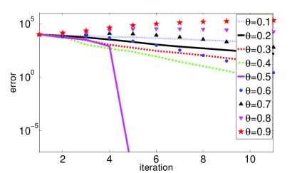
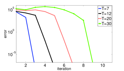
we show the convergence behavior for different values of the parameter $\theta$ for $T=16$ on the left, and on the right for the best parameter $\theta=\frac{1}{2}$ for different time window length $T$. Note that for some values of $\theta$ ($>0.7$) we get divergence. For the NNWR method, with the same initial guess, we show in Figure 2

Refer to caption Refer to caption

Figure 2: Convergence of NNWR with various values of $\theta$ for $T=16$ on the left, and for various lengths $T$ of the time window and $\theta=\frac{1}{4}$ on the right

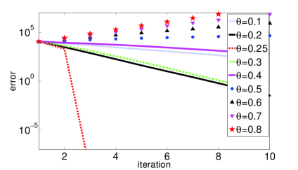
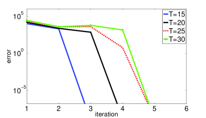
on the left the convergence curves for different values of $\theta$ for $T=16$, and on the right the results for the best parameter $\theta=\frac{1}{4}$ for different time window lengths $T$.

We finally compare in Figure 3 the performance of the DNWR and NNWR algorithms with the Schwarz Waveform Relaxation (SWR) algorithms from GHN with and without overlap.

Refer to caption Refer to caption

Figure 3: Comparison of DNWR, NNWR, and SWR for $T=4$ on the left, and $T=10$ on the right

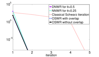
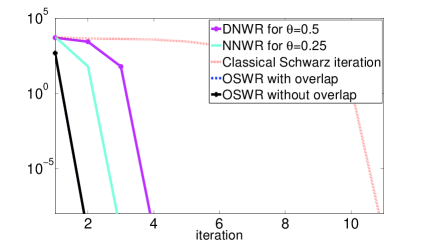
We consider the same model problem (4) with Dirichlet boundary conditions along the physical boundary. We use for the overlapping Schwarz variant an overlap of length $24\Delta x$, where $\Delta x=1/50$. We observe that the DNWR and NNWR algorithms converge as fast as the Schwarz WR algorithms for smaller time windows $T$. Due to the local nature of the Dirichlet-to-Neumann operator in 1d GHN , SWR converges in a finite number of iterations just like DNWR and NNWR. In higher dimensions, however, SWR will no longer converge in a finite number of steps, but DNWR and NNWR will GKM2 .

5 Conclusions

We introduced the DNWR and NNWR algorithms for the second order wave equation, and analyzed their convergence properties for the 1d case and a two subdomain decomposition. We showed that for a particular choice of the relaxation parameter, convergence can be achieved in a finite number of steps. Choosing the time window lengh carefully, these algorithms can be used to solve such problems in two iterations only. For a detailed analysis for the case of multiple subdomains, see GKM2 .

References

  • (1) Bjørhus, M.: A note on the convergence of discretized dynamic iteration. BIT pp. 291–296 (1995)
  • (2) Bjørstad, P.E., Widlund, O.B.: Iterative Methods for the Solution of Elliptic Problems on Regions Partitioned into Substructures. SIAM J. Numer. Anal. (1986)
  • (3) Bourgat, J.F., Glowinski, R., Tallec, P.L., Vidrascu, M.: Variational Formulation and Algorithm for Trace Operator in Domain Decomposition Calculations. In: T.F. Chan, R. Glowinski, J. Périaux, O.B. Widlund (eds.) Domain Decomposition Methods, pp. 3–16. SIAM (1989)
  • (4) Gander, M.J., Halpern, L.: Optimized Schwarz Waveform Relaxation for Advection Reaction Diffusion Problems. SIAM J. Numer. Anal. 45(2), 666–697 (2007)
  • (5) Gander, M.J., Halpern, L., Nataf, F.: Optimal Schwarz Waveform Relaxation for the One Dimensional Wave Equation. SIAM J. Numer. Anal. 41(5), 1643–1681 (2003)
  • (6) Gander, M.J., Kwok, F., Mandal, B.C.: Dirichlet-Neumann and Neumann-Neumann Waveform Relaxation Algorithms for Parabolic Problems. arXiv:1311.2709
  • (7) Gander, M.J., Kwok, F., Mandal, B.C.: Substructuring Waveform Relaxation Methods for the Heat and Wave Equations in Multiple subdomains. in Preparation
  • (8) Gander, M.J., Stuart, A.M.: Space-time continuous analysis of waveform relaxation for the heat equation. SIAM J. Sci. Comput. 19(6), 2014–2031 (1998)
  • (9) Giladi, E., Keller, H.: Space time domain decomposition for parabolic problems. Tech. Rep. 97-4, Center for research on parallel computation CRPC, Caltech (1997)
  • (10) Kwok, F.: Neumann-Neumann Waveform Relaxation for the Time-Dependent Heat Equation. Domain Decomposition in Science and Engineering XXI, Springer-Verlag (2013)
  • (11) Lelarasmee, E., Ruehli, A., Sangiovanni-Vincentelli, A.: The waveform relaxation method for time-domain analysis of large scale integrated circuits. IEEE Trans. Compt.-Aided Design Integr. Circuits Syst. 1(3), 131–145 (1982)
  • (12) Mandal, B.C.: A Time-Dependent Dirichlet-Neumann Method for the Heat Equation. Domain Decomposition in Science and Engineering XXI, Springer-Verlag (2013)
  • (13) Toselli, A., Widlund, O.B.: Domain Decomposition Methods, Algorithms and Theory. Springer (2005)