Bayesian and Maximum Likelihood Estimation for Gaussian Processes on an Incomplete Lattice

Abstract

This paper proposes a new approach for Bayesian and maximum likelihood parameter estimation for stationary Gaussian processes observed on a large lattice with missing values. We propose an MCMC approach for Bayesian inference, and a Monte Carlo EM algorithm for maximum likelihood inference. Our approach uses data augmentation and circulant embedding of the covariance matrix, and provides exact inference for the parameters and the missing data. Using simulated data and an application to satellite sea surface temperatures in the Pacific Ocean, we show that our method provides accurate inference on lattices of sizes up to $512\times 512$, and outperforms two popular methods: composite likelihood and spectral approximations.

Keywords: Circulant embedding; Data augmentation; Markov chain Monte Carlo; EM algorithm; Spatial statistics.

1 Introduction

Spatial lattice data are common in many fields, including environmental science, medical imaging and computer modeling. In these applications, a common approach is to treat the data as a realization of a stationary Gaussian process, and estimate the mean and covariance parameters using maximum likelihood or Bayesian methods. However, in practice the datasets are often extremely large and may have missing values. This makes likelihood inference impracticable, since exact Cholesky decompositions require $O(n^{3})$ operations, where $n$ is the number of observations. When the observations are taken on a two-dimensional lattice and the process is stationary, the exact likelihood cost is reduced to $O(n^{5/2})$ (Zimmerman, 1989). However, when the lattice is incomplete or has irregular boundaries, the computational cost is cubic in the number of observations.

To deal with this problem, many approximate likelihood methods have been proposed for large spatial datasets. Whittle (1954) introduced a spectral approximation for lattice data, which has been widely used. Fuentes (2007) extended the Whittle approximation to lattice data with missing values. Vecchia (1988) developed a composite likelihood method for unequally-spaced data, and Stein, Chi and Welty (2004) extended this approach to restricted maximum likelihood and provided asymptotic standard errors for the parameters. Kaufman, Schervish and Nychka (2008) proposed covariance tapering for likelihood estimation with unequally-spaced data. Other approaches for large datasets include Markov Random fields (Rue and Tjelmeland, 2002), fixed-rank kriging (Cressie and Johannesson, 2008), predictive processes (Banerjee, Gelfand, Finley and Sang, 2008), and predictive processes with tapering (Sang and Huang, 2012). However, all of these methods are approximate, so there remains a need for exact likelihood-based methods for large gridded datasets.

Recently, Stein, Chen and Anitescu (2013) proposed a stochastic method for unbiased estimation of the score function. The estimate converges to the true score function as the Monte Carlo sample size increases. However, at present there is no feasible ‘exact’ Bayesian Markov chain Monte Carlo solution for this problem, i.e., one that converges to samples from the correct posterior distribution as the number of iterations increases.

In this paper, we propose a new maximum likelihood and Bayesian approach for spatial data observed on a large, possibly incomplete, lattice. The key idea is to view the observed data as a partial realization from a Gaussian random field on a periodic lattice. We then treat the values at the unobserved locations on the periodic lattice as missing data, and impute them within a data augmentation procedure. Conditional on the parameters, the missing data are generated using conditional simulation techniques from the geostatistics literature. Conditional on the imputed data, we have a complete realization of a periodic process, and the complete-data likelihood can be computed efficiently using the fast Fourier transform. This iterative procedure is implemented for Bayesian inference using a Markov chain Monte Carlo (MCMC) algorithm, and for maximum likelihood estimation using a Monte Carlo expectation-maximization (EM) approach. Our approach is the first feasible exact MCMC for this setting.

We first use simulated data to show that the methods work well in practice, and compare them to existing methods. Under a range of sampling designs, including complete lattice, missing at random, and missing in blocks, we find that the Bayesian approach provides accurate, full probabilistic inference for the parameters on lattices up to size 512 $\times$ 512 (262,144 observations). Furthermore, our maximum likelihood approach outperforms both composite likelihood and spectral approximations in terms of recovering the true maximum likelihood estimate. Finally, we apply the MCMC method to a satellite image of sea surface temperatures, where observations are unavailable over land locations. The method is shown to provide accurate inference in this real-data application.

The rest of the paper is outlined as follows. In Section 2, we introduce the Gaussian process model for lattice data and describe the circulant embedding approach. Section 3 provides a MCMC method for Bayesian estimation and an EM algorithm for maximum likelihood estimation. The methods are illustrated in Section 4 with an extensive simulation study and an analysis satellite sea surface temperatures. Conclusions are given in Section 5.

2 Likelihood for Gaussian Processes

Let $\{Z(\mathbf{s}),\mathbf{s}\in D\subseteq\mathbb{R}^{d}\}$ be a stationary, isotropic Gaussian process with mean $\mu$ and covariance function $\mbox{cov}(Z(\mathbf{s}),Z(\mathbf{s}^{\prime}))=\sigma^{2}\varphi(|\mathbf{s}-\mathbf{s}^{\prime}|;\mbox{\boldmath$\theta$})$, where $\varphi(\cdot)$ is an isotropic correlation function, $|\cdot|$ is Euclidean distance and $\theta$ is a vector of unknown parameters. The goal is to estimate the parameters $(\mu,\sigma^{2},\mbox{\boldmath$\theta$})$ based on a realization of the process $\mathbf{Z}=(Z(\mathbf{s}_{1}),\ldots,Z(\mathbf{s}_{n}))^{\prime}$ at the locations $\mathbf{s}_{1},\ldots,\mathbf{s}_{n}$. The likelihood function is

$$p(\mathbf{Z}|\mu,\sigma^{2},\mbox{\boldmath$\theta$})\;=\;(2\pi\sigma^{2})^{-\frac{n}{2}}|\mathbf{\Sigma}(\mbox{\boldmath$\theta$})|^{-\frac{1}{2}}\exp\left\{-\frac{1}{2\sigma^{2}}(\mathbf{Z}-\mbox{\boldmath$\mu$})^{\prime}\mathbf{\Sigma}(\mbox{\boldmath$\theta$})^{-1}(\mathbf{Z}-\mbox{\boldmath$\mu$})\right\},$$ (1)

where $\mbox{\boldmath$\mu$}=\mu\mathbf{1}$, $\mathbf{1}=(1,\ldots,1)^{\prime}$ and $\mathbf{\Sigma}(\mbox{\boldmath$\theta$})$ is the $n\times n$ correlation matrix with elements $\mathbf{\Sigma}_{ij}(\mbox{\boldmath$\theta$})=\varphi(|\mathbf{s}_{i}-\mathbf{s}_{j}|;\mbox{\boldmath$\theta$})$. If the sampling locations are unequally spaced, the likelihood becomes computationally infeasible when $n$ is large (say, more than a few thousand), because the determinant requires $O(n^{3})$ operations to compute. If the observations are on a rectangular lattice with no missing data, then $\mathbf{\Sigma}(\mbox{\boldmath$\theta$})$ is block Toeplitz with Toeplitz blocks, which reduces the cost of the likelihood to $O(n^{5/2})$ (Zimmerman, 1989). However, if the observations are on an incomplete lattice (i.e., with missing data or non-rectangular boundaries), then $\mathbf{\Sigma}(\mbox{\boldmath$\theta$})$ has no special form, and the exact likelihood requires $O(n^{3})$ operations.

In this paper, we assume that the data are observed are on a $2-$dimensional lattice of size $n_{1}\times n_{2}$. We allow for missing data or irregular boundaries, so the lattice may be incomplete. To implement our estimation approach, we embed the domain in a larger lattice of size $N_{1}\times N_{2}$, where $N_{1}=2rn_{1}$ and $N_{2}=2rn_{2}$ and $r\geq 1$. We consider the periodic extension of $\varphi(h)$ in two dimensions with period $2r$ in each coordinate. Consider the random vector of length $N=N_{1}N_{2}$ defined over the embedding lattice. The covariance matrix of this random vector is block circulant with circulant blocks, which allows it to be diagonalized in $O(N\log N)$ operations. This leads to a data augmentation approach where we impute the random field at the unobserved locations on the embedding lattice, and then compute the complete data likelihood efficiently in $O(N\log N)$ operations. The approach is detailed below.

2.1 Circulant Embedding

Circulant embedding was proposed by Wood and Chan (1994) and Dietrich and Newsam (1997) as a method for simulating stationary Gaussian random fields on a large lattice. The main idea of this approach is to embed the original $n_{1}\times n_{2}$ grid in $[0,s]^{2}$ in a larger lattice of size $N_{1}\times N_{2}$, in $[0,2rs]^{2}$, where $r\geq 1$, $N_{1}=2rn_{1}$, $N_{2}=2rn_{2}$, and $N_{1}$ and $N_{2}$ are highly composite numbers. We assume throughout the paper that $s=1/\sqrt{2}\approx 0.707$. Following the notation in Stein (2002) and Gneiting, Ševčíková, Percival, Schlather and Jiang (2006), we define $P_{s}\varphi$ as the function on $\mathbb{R}^{2}$ that has period $2s$ in each coordinate, such that $P_{s}\varphi(\mathbf{s})=\varphi(|\mathbf{s}|)$, for $\mathbf{s}\in[-s,s]^{2}$, and let $\mathbf{C}$ denote the $N\times N$ covariance matrix obtained by evaluating $P_{s}\varphi$ over the $N=N_{1}N_{2}$ points on the embedding lattice ordered lexicographically. Since $P_{s}\varphi$ is periodic and the domain is a rectangular grid, $\mathbf{C}$ is block circulant matrix with circulant blocks (BCCB). This allows the matrix to be diagonalized in $O(N\log N)$ operations using the fast Fourier transform (FFT).

To simulate $\mathbf{Z}\sim\mathcal{N}(\mathbf{0},\mathbf{C})$, we first compute the eigenvalues of $\mathbf{C}$, $\mbox{\boldmath$\lambda$}=(\lambda_{1},\ldots,\lambda_{N})$, then generate an independent random vector with variances proportional to the eigenvalues, and then apply an FFT to the random vector to obtain a Gaussian random field over the embedding grid. The issue is how to choose the value of $r$. The standard embedding approach is to choose the smallest value of $r>1$ for which $N_{1}=2rn_{1}$ and $N_{2}=2rn_{2}$ are highly composite numbers. For some values of $r$, however, this may result in a non positive-definite matrix $\mathbf{C}$. To avoid this problem, Wood and Chan (1994) proposed increasing the value of $r$ until $\mathbf{C}$ is positive definite; however, this often requires a very large value of $r$, which makes computation prohibitive.

Stein (2002) proposed an alternative approach to ensure positive definite embeddings. Gneiting, Ševčíková, Percival, Schlather and Jiang (2006) labeled this method cutoff embedding and explored the limits of when the method can be used. For a given isotropic correlation function $\varphi(\cdot)$, Stein (2002) considers the modified correlation function

$$\rho(h)=\left\{\begin{tabular}[]{ll}$\varphi(h)$&if $0\leq h<1$;\\ $\psi(h)$&if $1\leq h<r$;\\ $0$&if $h\geq r$,\end{tabular}\right.$$

where $h$ is Euclidean distance, and $r>1$ is the ‘cutoff radius’ and $\psi(h)$ is a function chosen to make $\rho(h)$ differentiable at $r$. The compact support of $\rho(\cdot)$ ensures that the periodic function $P_{r}\rho$ is positive definite, providing that $\varphi(\cdot)$ satisfies certain conditions (Gneiting et al., 2006). Stein (2002) and Gneiting et al. (2006) chose $\psi(h)$ to be a quadratic or square root function. The circulant embedding approach is then applied using the modified covariance function $P_{r}\rho$, and the resulting covariance matrix $\mathbf{C}$ is guaranteed to be positive definite.

Figure 1 illustrates the minimal embedding and extended embedding schemes for a square lattice with missing observations. Here, the original lattice is $16\times 16$, with data missing in a circle or disk shape. Panel (a) shows the minimal embedding scheme, where the embedding lattice is of size $32\times 32$. Panel (b) illustrates an extended embedding scheme with a ‘cutoff’ radius of $r=1.5s\approx 1.06$ and a embedding grid of size $48\times 48$.

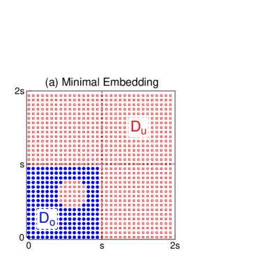
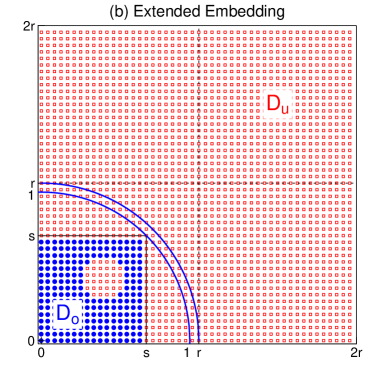
Figure 1: Circulant embedding schemes for a square lattice. Closed circles denote observed locations; open squares denote unobserved locations. The original domain is $16\times 16$ on $[0,s]^{2}$ where $s=1/\sqrt{2}\approx 0.707$, with data missing in a disk shape. (a) Minimal embedding scheme with a $32\times 32$ embedding lattice. (b) Extended embedding scheme with $r=1.5s\approx 1.06$ and a $48\times 48$ embedding lattice.

2.2 BCCB Matrices

If $\mathbf{C}$ is the covariance matrix for a periodic, stationary random field on a $2-$dimensional $N_{1}\times N_{2}$ complete lattice with points ordered lexicographically, then it has a block circulant form with circulant blocks (BCCB). Then, $\mathbf{C}=\mathbf{F}\mathbf{\Lambda}\mathbf{F}^{*}$, where $\mathbf{F}$ is the $2-$dimensional Fourier transform matrix, $\mathbf{F}^{*}$ is the corresponding inverse Fourier transform matrix, and $\mathbf{\Lambda}=\mbox{diag}(\lambda_{1},\ldots,\lambda_{N})$ is the diagonal matrix of eigenvalues. BCCB matrices have a number of computational advantages, namely that eigenvalues, matrix-vector multiplications and quadratic forms can be computed efficiently in $O(N\log N)$ operations by exploiting the FFT, and they have a storage cost of $O(N)$. The properties of BCCB matrices are summarized in Appendix A. Also see Kozintsev (1999) for an excellent summary of BCCB matrices for Gaussian random fields.

2.3 Unconditional Simulation

Exact simulation of periodic, stationary Gaussian random fields on a grid can be performed efficiently using the circulant embedding approach of Wood and Chan (1994), Dietrich and Newsam (1997) and Stein (2002). Because the covariance matrix $\mathbf{C}$ is BCCB, unconditional simulations can be obtained in $O(N\log N)$ operations by exploiting the fast Fourier transform. Specifically, to generate draws $\mathbf{Z}\sim\mathcal{N}(\mathbf{0},\mathbf{C})$, we set $\mathbf{Z}=\mathbf{F}\mathbf{\Lambda}^{1/2}\mbox{\boldmath$\epsilon$}$, where $\mbox{\boldmath$\epsilon$}\sim\mathcal{CN}(\mathbf{0},\mathbf{I})$ is a complex normal random vector, generated as $\mbox{\boldmath$\epsilon$}=\mbox{\boldmath$\epsilon$}_{1}+i\mbox{\boldmath$\epsilon$}_{2}$, with $\mbox{\boldmath$\epsilon$}_{1},\mbox{\boldmath$\epsilon$}_{2}\sim\mathcal{N}(\mathbf{0},\mathbf{I})$. The vector $\mathbf{Z}=\mathbf{Z}_{1}+i\mathbf{Z}_{2}$, yields two independent draws $\mathbf{Z}_{1}$ and $\mathbf{Z}_{2}$ from $\mathcal{N}(\mathbf{0},\mathbf{C})$.

2.4 Likelihood Function

Let $\mathbf{Z}$ be a random vector representing a stationary, periodic random field on a lattice, then it has distribution $\mathbf{Z}\sim\mathcal{N}(\mbox{\boldmath$\mu$},\sigma^{2}\mathbf{C}(\mbox{\boldmath$\theta$}))$, where $\mathbf{C}(\mbox{\boldmath$\theta$})$ is BCCB. Let $\mathbf{\Theta}=(\mu,\sigma^{2},\mbox{\boldmath$\theta$})$ denote the set of unknown mean and covariance parameters. The loglikelihood function for the complete data is (ignoring constants)

$$\log p(\mathbf{Z}|\mathbf{\Theta}) = -\frac{N}{2}\log\sigma^{2}-\frac{1}{2}\log|\mathbf{C}(\mbox{\boldmath$\theta$})|-\frac{1}{2\sigma^{2}}(\mathbf{Z}-\mbox{\boldmath$\mu$})^{\prime}\mathbf{C}(\mbox{\boldmath$\theta$})^{-1}(\mathbf{Z}-\mbox{\boldmath$\mu$}),$$

$$= -\frac{N}{2}\log\sigma^{2}-\frac{1}{2}\sum_{i=1}^{N}\log\lambda_{i}-\frac{1}{2\sigma^{2}}\left(\mathbf{\Lambda}^{-1/2}\mathbf{F}^{*}\mbox{\boldmath$\epsilon$}\right)^{\prime}\left(\mathbf{\Lambda}^{-1/2}\mathbf{F}^{*}\mbox{\boldmath$\epsilon$}\right)$$

where $\mbox{\boldmath$\epsilon$}=\mathbf{Z}-\mbox{\boldmath$\mu$}$. The loglikelihood can be computed efficiently using fast Fourier transforms. We first compute the eigenvalues of $\mathbf{C}(\mbox{\boldmath$\theta$})$ using a 2-dimensional FFT. The determinant is then computed as the product of eigenvalues. The quadratic form is computed using an FFT followed by a vector-vector multiplication. Therefore, the overall cost to compute the complete-data loglikelihood is $O(N\log N)$ operations.

2.5 Conditional Simulation

Our estimation approach requires an efficient method for generating conditional simulations of the missing data given the observed data and the parameters. Let $D_{o}$ and $D_{u}$ denote the observed and unobserved locations on the embedding lattice, and $D=D_{o}\cup D_{u}$ denote all locations on the embedding lattice. Let $\mathbf{Z}_{o}=\{Z(\mathbf{s}):\mathbf{s}\in D_{o}\}$ and $\mathbf{Z}_{u}=\{Z(\mathbf{s}):\mathbf{s}\in D_{u}\}$ denote the observed and unobserved data on the embedding lattice. and let $\mathbf{Z}=\{Z(\mathbf{s}):\mathbf{s}\in D\}$ denote the complete data. Suppose $\mathbf{Z}\sim\mathcal{N}(\mbox{\boldmath$\mu$},\mathbf{C})$ and can be partitioned as

$$\left(\begin{tabular}[]{c}$\mathbf{Z}_{o}$\\ $\mathbf{Z}_{u}$\end{tabular}\right)\sim\mathcal{N}\left(\left(\begin{tabular}[]{c}$\mbox{\boldmath$\mu$}_{o}$\\ $\mbox{\boldmath$\mu$}_{u}$\end{tabular}\right),\left(\begin{tabular}[]{cc}$\mathbf{C}_{oo}$&$\mathbf{C}_{ou}$\\ $\mathbf{C}_{uo}$&$\mathbf{C}_{uu}$\end{tabular}\right)\right)$$ (2)

where $n$ is the number of observed data, $N-n$ the number of unobserved data, and $N$ is the total number of lattice points. The conditional distribution for the missing data given the observed data is

$$\mathbf{Z}_{u}|\mathbf{Z}_{o}\sim\mathcal{N}\left(\mbox{\boldmath$\mu$}_{u}+\mathbf{C}_{uo}\mathbf{C}_{oo}^{-1}(\mathbf{Z}_{o}-\mbox{\boldmath$\mu$}_{o}),\mathbf{C}_{u|o}\right),$$ (3)

where $\mathbf{C}_{u|o}=\mathbf{C}_{uu}-\mathbf{C}_{uo}\mathbf{C}_{oo}^{-1}\mathbf{C}_{ou}$. Direct simulation from this distribution is infeasible when $N$ is large, because of the cost of computing and storing the conditional covariance matrix $\mathbf{C}_{u|o}$, and its Cholesky decomposition, which require $O(N^{3})$ and $O(N^{2})$ operations, respectively.

We generate conditional simulations using the substitution sampling approach of Matheron (1976). This method is more efficient than direct simulation, because it avoids the conditional covariance matrix and its Cholesky decomposition. The method proceeds in two steps. We first simulate the complete random field from its unconditional distribution, $\widetilde{\mathbf{Z}}\sim\mathcal{N}(\mbox{\boldmath$\mu$},\mathbf{C})$, using the approach described in Section 2.3. We then obtain the conditional simulation $\mathbf{Z}^{*}_{u}$ by defining

$$\mathbf{Z}^{*}_{u}=\widetilde{\mathbf{Z}}_{u}+\mathbf{C}_{uo}\mathbf{C}_{oo}^{-1}(\mathbf{Z}_{o}-\widetilde{\mathbf{Z}}_{o}).$$ (4)

It is straightfoward to show that $\mathbf{Z}^{*}_{u}\sim p(\mathbf{Z}_{u}|\mathbf{Z}_{o},\mathbf{\Theta})$; i.e., it has the mean and covariance given in (3). For a proof, see Chilès and Delfiner (2012). Note that $\mathbf{Z}^{*}_{u}$ has the same form as the conditional mean given in (3), but with the simulated field $\widetilde{\mathbf{Z}}$ substituted for $\mu$. To obtain the conditional simulation, we must first solve the system

$$\mathbf{C}_{oo}\mathbf{x}=\mbox{\boldmath$\eta$},\mbox{ where }\mbox{\boldmath$\eta$}=\mathbf{Z}_{o}-\widetilde{\mathbf{Z}}_{o}.$$ (5)

It is infeasible to solve this directly when $n$ is large, as it requires $O(n^{3})$ operations. Instead we use an iterative method to solve the system, which is described below. After solving the system, the conditional simulation is obtained by computing $\mathbf{w}_{u}=\mathbf{C}_{uo}\mathbf{x}$, which can be done efficiently by exploiting the form of $\mathbf{C}$, and then setting $\mathbf{Z}^{*}_{u}=\widetilde{\mathbf{Z}}_{u}+\mathbf{w}_{u}$.

2.6 Preconditioned Conjugate Gradient

We use the preconditioned conjugate gradient (PCG) algorithm (Golub and Van Loan, 1996) to solve the system (5). The PCG is an iterative method that solves the modified system

$$\mathbf{M}^{-1}\mathbf{C}_{oo}\mathbf{x}=\mathbf{M}^{-1}\mbox{\boldmath$\eta$}~{}~{}\mbox{where}~{}~{}\mbox{\boldmath$\eta$}=\mathbf{Z}_{o}-\widetilde{\mathbf{Z}}_{o},$$ (6)

where $\mathbf{M}^{-1}$ is an $n\times n$ preconditioner matrix. The solution to the modified system is the same as the original solution, but the use of the preconditioner speeds up convergence of the algorithm (see Appendix B). Convergence to the exact solution is guaranteed within $n$ iterations; however, a good approximation can usually be obtained in far fewer iterations. The algorithm is stopped at the iteration $k$ when the residual vector $\mathbf{r}_{k}=\mbox{\boldmath$\eta$}-\mathbf{C}_{oo}\mathbf{x}_{k}$, is smaller than a specified tolerance. We use the criterion $|\mathbf{r}_{k}|/|\mathbf{r}_{0}|<\epsilon$, where $\epsilon$ is a specified error tolerance.

The PCG requires only matrix-vector multiplications of the form $\mathbf{C}_{oo}\mathbf{x}$ and $\mathbf{M}^{-1}\mathbf{x}$. The former can be computed efficiently by exploiting the block circulant structure of $\mathbf{C}$. Suppose $\mathbf{C}$ is partitioned as in (2). To compute $\mathbf{C}_{oo}\mathbf{x}$, we pad the vector $\mathbf{x}$ with zeros, i.e., $\mathbf{x}^{*}=(\mathbf{x}^{\prime},\mathbf{0}^{\prime})^{\prime}$, then multiply $\mathbf{w}=\mathbf{C}\mathbf{x}^{*}$, and the result is obtained in the first $n$ elements of $\mathbf{w}$:

$$\mathbf{w}=\mathbf{C}\mathbf{x}^{*}=\left(\begin{tabular}[]{cc}$\mathbf{C}_{oo}$&$\mathbf{C}_{ou}$\\ $\mathbf{C}_{uo}$&$\mathbf{C}_{uu}$\end{tabular}\right)\left(\begin{tabular}[]{c}$\mathbf{x}$\\ $\mathbf{0}$\end{tabular}\right)=\left(\begin{tabular}[]{c}$\mathbf{C}_{oo}\mathbf{x}$\\ $\mathbf{C}_{uo}\mathbf{x}$\end{tabular}\right)$$

This procedure is also used to compute $\mathbf{C}_{uo}\mathbf{x}$, but the result is obtained in the last $N-n$ elements of $\mathbf{w}$. This step is needed in the conditional simulations after solving the system. Each multiplication of the form $\mathbf{C}\mathbf{x}$ requires two fast Fourier transforms, which require $N\log N$ operations. Each PCG iteration requires one $\mathbf{C}\mathbf{x}$ multiplication. Therefore, the total computational cost for one conditional simulation is $O(IN\log N)$, where $I$ is the number of PCG iterations.

2.7 Preconditioners

The performance of the PCG depends critically on the choice of preconditioner. Ideally, the preconditioner should satisfy three criteria: $\mathbf{M}^{-1}\mathbf{C}_{oo}$ should have a small condition number; $\mathbf{M}^{-1}\mathbf{x}$ can be multiplied quickly; and $\mathbf{M}^{-1}$ should have a low storage cost. Common choices for preconditioners include circulant/block circulant matrices, block diagonal matrices, incomplete LU or Cholesky decompositions, and sparse matrices (see Golub and Van Loan, 1996).

In our analysis, we propose a new preconditioner based on the composite likelihood methods of Vecchia (1988) and Stein et al. (2004). For this method, the observed data $\mathbf{Z}$ are partitioned into $q$ blocks and the likelihood is approximated by a product of conditional normal densities $p(\mathbf{A}_{j}\mathbf{Z}|\mathbf{B}_{j}\mathbf{Z})$, $j=1,\ldots,q$, where $\mathbf{A}_{j}$ and $\mathbf{B}_{j}$ are matrices of zeros and ones that define the prediction and conditioning sets for block $j$. The sets are chosen to be small so that the conditional moments can be computed and stored efficiently. Since each conditional density is Gaussian, the likelihood approximation corresponds to a multivariate normal density $\mathcal{N}(\mathbf{Z}|\mathbf{0},\mathbf{V})$, where $\mathbf{V}^{-1}=\mathbf{L}^{\prime}\mathbf{D}\mathbf{L}$, where $\mathbf{L}$ and $\mathbf{D}$ are sparse $n\times n$ matrices containing the regression coefficients and precision matrices for the conditional distributions (see Appendix C). The approximation assumes that $\mathcal{N}(\mathbf{Z}|\mathbf{0},\mathbf{V})\approx\mathcal{N}(\mathbf{Z}|\mathbf{0},\mathbf{C}_{oo})$. Therefore, we choose $\mathbf{V}^{-1}$ as our preconditioner. We then only need to specify the prediction and conditioning sets. In our appplications, we choose prediction sets of size 4 and conditioning sets of size 18, 33 or 52.

We have also developed a number of other preconditioners, including BCCB, block diagonal, and sparse covariance/precision matrices based on Whittle’s approximation, covariance tapering and Markov random fields, respectively. One preconditioner that works quite well is the observed block of the complete-data precision matrix, i.e., $(\mathbf{C}^{-1})_{oo}$. Since the inverse of a BCCB matrix is also BCCB, it has a storage cost of $O(N)$ and matrix-vector multiplications are computed efficiently using FFTs. We found that this preconditioner works well for complete or nearly complete lattices, but less well with large amounts of missing data. However, we found that all of these choices were generally outperformed by the Vecchia preconditioner in terms of convergence rate and run time.

In the next section, we propose two estimation algorithms based on the ideas of circulant embedding and conditional simulation. First, we propose a MCMC algorithm for Bayesian inference. Second, we introduce a Monte Carlo EM algorithm for maximum likelihood estimation. We emphasize that both of the proposed algorithms are exact, up to Monte Carlo error.

3 Parameter Estimation

3.1 Bayesian Estimation

For the Bayesian analysis, we specify a prior distribution for the unknown parameters, $\pi(\mathbf{\Theta})$, and make inference based on the joint posterior distribution

$$\pi(\mathbf{\Theta},\mathbf{Z}_{u}|\mathbf{Z}_{o})\propto p(\mathbf{Z}|\mathbf{\Theta})\,\pi(\mathbf{\Theta}),$$

where $\mathbf{Z}=(\mathbf{Z}_{o},\mathbf{Z}_{u})$ denotes the complete data. This joint posterior distribution is typically unavailable in closed form. Therefore, we propose a Markov chain Monte Carlo (MCMC) algorithm to sample from it. Specifically, we propose a two-block Gibbs sampler that alternates between updating the missing data and the parameters. Given initial parameter values, $\mathbf{\Theta}^{0}$, the MCMC algorithm proceeds as follows for $i=1,\ldots,M$:

1. Generate $\mathbf{Z}_{u}^{i}\sim p(\mathbf{Z}_{u}|\mathbf{Z}_{o},\mathbf{\Theta}^{i-1})$.

2. Generate $\mathbf{\Theta}^{i}\sim\pi(\mathbf{\Theta}|\mathbf{Z}^{i})$.

The missing data are updated using conditional simulation methods described in Section 2.5. The parameters are updated using a block Metropolis-Hastings step, described below.

Given the complete data, the parameters are generated from their conditional distribution $\pi(\mathbf{\Theta}|\mathbf{Z})\propto p(\mathbf{Z}|\mathbf{\Theta})\pi(\mathbf{\Theta})$. This distribution is easy to evaluate, but is generally unavailable in closed form due to the nonlinearity of $\theta$ in the determinant and the quadratic form. Bayesian MCMC approaches to estimate covariance parameters in spatial Gaussian processes include Ecker and Gelfand (1997), who proposed a Metropolis algorithm and Agarwal and Gelfand (2005), who proposed a slice sampling approach. Here, we use a Metropolis-Hastings scheme to update the parameters, which proceeds as follows.

1. Generate $\mathbf{\Theta}^{*}$ from a proposal distribution $q(\mathbf{\Theta}|\mathbf{\Theta}^{i})$.

2. Accept $\mathbf{\Theta}^{*}$ with probability

   $$\min\left\{1,\frac{p(\mathbf{Z}|\mathbf{\Theta}^{*})\,\pi(\mathbf{\Theta}^{*})}{p(\mathbf{Z}|\mathbf{\Theta}^{i})\,\pi(\mathbf{\Theta}^{i})}\frac{q(\mathbf{\Theta}^{i}|\mathbf{\Theta}^{*})}{q(\mathbf{\Theta}^{*}|\mathbf{\Theta}^{i})}\right\}.$$

The computational cost to generate the missing data is $O(IN\log N)$, and the cost to update the parameters is $O(N\log N)$. Hence the cost for each iteration of the Gibbs sampler is $O(IN\log N)$ operations, and the total cost for $M$ iterations of the sampler is $O(MIN\log N)$.

The Bayesian approach also provides inference for the random field at missing locations via the posterior predictive distribution (see Handcock and Stein, 1993). If the missing data lie on the original lattice or the embedding lattice, the MCMC algorithm automatically generates samples from their distribution as part of the imputation step.

3.2 Maximum Likelihood Estimation

For maximum likelihood (ML) estimation, we propose an expectation-maximization (EM) algorithm Dempster, Laird and Rubin (1977) to obtain the maximum likelihood estimate $\widehat{\mathbf{\Theta}}=\arg\max_{\mathbf{\Theta}}p(\mathbf{Z}_{o}|\mathbf{\Theta})$. The algorithm iterates between the E-step and M-step until convergence. In the E-step, we calculate the expected complete-data loglikelihood given the observed data and the current parameter, $\mathbf{\Theta}^{t}$:

$$Q(\mathbf{\Theta}|\mathbf{\Theta}^{t})=\int\log p(\mathbf{Z}|\mathbf{\Theta})p(\mathbf{Z}|\mathbf{Z}_{o},\mathbf{\Theta}^{t})d\mathbf{Z}.$$ (7)

In the M-step, we maximize this function to obtain the next parameter value, $\mathbf{\Theta}^{t+1}$. Under the Gaussian model (2), the distribution for the complete data is $\mathbf{Z}|\mathbf{\Theta}\sim\mathcal{N}(\mbox{\boldmath$\mu$}(\mathbf{\Theta}),\mathbf{C}(\mathbf{\Theta}))$, and the conditional distribution for the complete data is $\mathbf{Z}|\mathbf{Z}_{o},\mathbf{\Theta}^{t}\sim\mathcal{N}(\widetilde{}\mbox{\boldmath$\mu$}(\mathbf{\Theta}^{t}),\widetilde{\mathbf{C}}(\mathbf{\Theta}^{t}))$. Suppressing dependence on parameters, and ignoring constants, the expectation (7) is

$$Q(\mathbf{\Theta}|\mathbf{\Theta}^{t}) = -\frac{1}{2}\log|\mathbf{C}|-\frac{1}{2}E\left\{(\mathbf{Z}-\mbox{\boldmath$\mu$})^{\prime}\mathbf{C}^{-1}(\mathbf{Z}-\mbox{\boldmath$\mu$})|\mathbf{Z}_{o},\mathbf{\Theta}^{t}\right\}$$ (8)

$$= -\frac{1}{2}\log|\mathbf{C}|-\frac{1}{2}\left\{\mathrm{tr}(\mathbf{C}^{-1}\widetilde{\mathbf{C}})+(\widetilde{\mbox{\boldmath$\mu$}}-\mbox{\boldmath$\mu$})^{\prime}\mathbf{C}^{-1}(\widetilde{\mbox{\boldmath$\mu$}}-\mbox{\boldmath$\mu$})\right\}.$$ (9)

Note that the trace term in (9) involves $\widetilde{\mathbf{C}}$, the conditional covariance matrix for the complete data. This matrix consists of $\widetilde{\mathbf{C}}_{u|o}$ in the lower diagonal block, and zeros elsewhere, and does not have a BCCB form. Thus, it is infeasible to compute $\widetilde{\mathbf{C}}$ when $n$ is large and therefore $Q$ cannot be evaluated exactly. Instead, we propose a Monte Carlo approach, where we approximate the expected loglikelihood (8) by

$$\widehat{Q}(\mathbf{\Theta}|\mathbf{\Theta}^{t})=-\frac{1}{2}\log|\mathbf{C}|-\frac{1}{2}\left\{\frac{1}{M}\sum_{i=1}^{M}(\mathbf{Z}^{(i)}-\mbox{\boldmath$\mu$})^{\prime}\mathbf{C}^{-1}(\mathbf{Z}^{(i)}-\mbox{\boldmath$\mu$})\right\},$$ (10)

where $\mathbf{Z}^{(1)},\ldots,\mathbf{Z}^{(M)}\sim p(\mathbf{Z}|\mathbf{Z}_{o},\mathbf{\Theta}^{t})$ are conditional simulations of the complete data generated using the current parameter value $\mathbf{\Theta}^{t}$. We then maximize $\hat{Q}$ to obtain the new parameter value, $\mathbf{\Theta}^{t+1}$. The Monte Carlo expectation avoids computing the conditional covariance matrix, and requires only a determinant and $M$ quadratic forms involving the matrix $\mathbf{C}$. Therefore, $\hat{Q}$ can be computed for large $n$. Given an initial parameter $\mathbf{\Theta}^{0}$, the EM algorithm proceeds as follows for $t=0,1,\ldots,T$.

1. (E-step) Generate $\mathbf{Z}_{u}^{(1)},\ldots,\mathbf{Z}_{u}^{(M)}\sim p(\mathbf{Z}_{u}|\mathbf{Z}_{o},\mathbf{\Theta}^{t}).$

2. (M-step) Update $\mathbf{\Theta}^{t+1}=\arg\underset{\mathbf{\Theta}}{\max}\,\widehat{Q}(\mathbf{\Theta}|\mathbf{\Theta}^{t})$.

In Step 1 of the EM algorithm, we generate $M$ conditional simulations using the current parameter $\mathbf{\Theta}^{t}$ using the approach described in Section 2.5. In Step 2, we maximize the expected complete-data loglikelihood using numerical optimization methods such as Newton-Raphson or the Nelder-Mead simplex algorithm.

4 Examples

4.1 Simulation Study

To study the performance of the estimation algorithms, we first conduct a detailed simulation study using different lattice sizes and missingness patterns. We generate data from a stationary, isotropic Gaussian process, with mean $\mu$ and covariance $\mathrm{Cov}(Z(\mathbf{s}),Z(\mathbf{s}^{\prime}))=\sigma^{2}\varphi(|\mathbf{s}-\mathbf{s}^{\prime}|)$, where $\varphi(\cdot)$ is a powered exponential correlation with microscale noise Cressie (1993):

$$\varphi(h)=\exp\left\{-(h/\lambda)^{\alpha}\right\}+c\mathbbm{1}_{(h=0)}.$$ (11)

Here $\sigma^{2}$ is the partial sill parameter, $\lambda>0$ is the spatial range parameter, $\alpha\in(0,2]$ is the shape parameter, $c\geq 0$ is the ratio between the microscale and macroscale variation, and $\mathbbm{1}_{A}$ is an indicator for the event $A$. The parameter $\tau^{2}=c\sigma^{2}$ represents the variance of the microscale noise. The model contains the exponential ($\alpha=1$) and squared exponential ($\alpha=2$) covariances as special cases. For the simulation study, we fix $c$ at its true value and estimate the parameters $\mu$, $\sigma^{2}$ and $\mbox{\boldmath$\theta$}=(\lambda,\alpha)$, using the methods from Section 3. This is done to make the simulation study feasible while still allowing a nugget effect, which is often present in practice.

For circulant embedding, we use a variant of the cutoff embedding approach described in Section 2, with the modified correlation function

$$\rho(h)=\left\{\begin{tabular}[]{ll}$\exp\{-(h/\lambda)^{\alpha}\}+c\mathbbm{1}_{(h=0)},$&$0\leq h<1$;\\ $a+b(h-r)^{2},$&$1\leq h<r$;\\ $a,$&$h\geq r$,\end{tabular}\right.$$ (12)

where $r>1$, and $a=\exp\{-(1/\lambda)^{\alpha}\}/\{1-(r-1)/2\lambda\}$ and $b=\exp\{-(1/\lambda)^{\alpha}\}/\{2\lambda(r-1)\}$ are chosen to make $\rho(h)$ differentiable at $1$ and $\rho^{\prime}(r)=0$. This approach is similar to cutoff embedding with a quadratic function $\psi(h)$, but here $r$ is selected by the user, and $\rho(h)$ is set to a constant rather than zero for $h\geq r$. While this approach does not guarantee non-negative definite embeddings, it leads to fewer violations than standard embedding, while allowing for a much smaller value of $r$ than required for cutoff embedding.

The value of $r$ required for a non-negative definite embedding depends on the parameters $\lambda,\alpha,c$. If these parameters were known, we could choose $r$ by trial and error. However, in the context of an MCMC or EM algorithm, the parameters are unknown and changing at each iteration. One possible solution is to adaptively update $r$ (and the size of the embedding grid) along with the parameters. However, this implies a variable-dimensional state space, which requires reversible jump or other trans-dimensional MCMC methods, which are difficult to use in high-dimensional settings. To simplify estimation, we hold $r$ fixed throughout the estimation algorithm, and choose its value based on prior information, with subsequent modifications made based on a few trial runs of the algorithm.

For the simulation study, we generate data on a $n_{1}\times n_{1}$ lattice on $[0,s]^{2}$, where $s=1/\sqrt{2}$. The true parameter values are $\sigma^{2}=4$, $\lambda=0.10$, $\alpha=1$, $c=0.01$ and $\mu=10$, which corresponds to an exponential covariance with small microscale variation. We use the modified correlation function (12) with $r=1.5s\approx 1.06$, and an embedding lattice of size $3n_{1}\times 3n_{1}$ on $[0,3s]^{2}$. The ‘cutoff’ radius $r$ is about 10 times larger than the spatial range parameter $\lambda$. We focus on the behavior of the algorithms over a fixed spatial region as the grid becomes increasingly dense. We consider observation lattices of size $n_{1}=$ 32, 64, 128, 256 and 512 with corresponding embedding lattices of size $N_{1}=$ 96, 192, 384, 768, and 1536, and three different missingness patterns: complete lattice, 10% missing at random, and 10% missing disk.

4.1.1 Bayesian Analysis

For the Bayesian analysis, we assume a prior distribution of the form $\pi(\mu,\sigma^{2},\mbox{\boldmath$\theta$})\propto\pi(\mbox{\boldmath$\theta$})/\sigma^{2}$, corresponding to a noninformative Jeffreys’ prior for the mean and variance, $\pi(\mu,\sigma^{2})\propto 1/\sigma^{2}$, and a prior for the correlation parameters, $\pi(\mbox{\boldmath$\theta$})=\pi(\lambda)\pi(\alpha)$, where

$$\pi(\lambda)=\frac{0.5}{(1+0.5\lambda)^{2}}$$

and $\pi(\alpha)=\mathcal{U}(0,2)$. Note that a proper prior for the range parameter is needed to ensure a proper posterior (Berger, De Oliveira and Sansó, 2001). We choose a proper prior for $\lambda$ with a mode of zero, a median of two, and a long right tail, reflecting our belief that large values of the range are less likely than small ones. A similar prior was used by Handcock and Stein (1993) and Handcock and Wallis (1994). This prior is uninformative for $0.5\lambda/(1+0.5\lambda)$ on $[0,1]$. The prior for the shape parameter is proper and uniform over its support $\alpha\in(0,2]$.

Let $\mathbf{Z}$ denote the complete data over the embedding lattice. Then $\mathbf{Z}\sim\mathcal{N}(\mu\mathbf{1},\sigma^{2}\mathbf{C}(\mbox{\boldmath$\theta$}))$, where $\mathbf{C}(\mbox{\boldmath$\theta$})$ is the correlation matrix obtained by evaluating $P_{r}\rho(h)$ over the points on the embedding lattice. Multiplying the prior distribution and the complete-data likelihood, we obain the full conditional posterior for the parameters:

$$\pi(\mu,\sigma^{2},\mbox{\boldmath$\theta$}|\mathbf{Z})~{}\propto~{}(\sigma^{2})^{-\frac{N}{2}-1}|\mathbf{C}(\mbox{\boldmath$\theta$})|^{-\frac{1}{2}}\exp\left\{-\frac{1}{2\sigma^{2}}\left[\frac{(\mu-\hat{\mu})^{2}}{(\mathbf{1}^{\prime}\mathbf{C}(\mbox{\boldmath$\theta$})^{-1}\mathbf{1})^{-1}}+S^{2}(\mbox{\boldmath$\theta$})\right]\right\}\,\pi(\mbox{\boldmath$\theta$}),$$

where $\hat{\mu}=\mathbf{1}^{\prime}\mathbf{C}(\mbox{\boldmath$\theta$})^{-1}\mathbf{Z}/(\mathbf{1}^{\prime}\mathbf{C}(\mbox{\boldmath$\theta$})^{-1}\mathbf{1})=\mathbf{1}^{\prime}\mathbf{Z}/N=\bar{Z}$ and $S^{2}(\mbox{\boldmath$\theta$})=(\mathbf{Z}-\hat{\mu}\mathbf{1})^{\prime}\mathbf{C}(\mbox{\boldmath$\theta$})^{-1}(\mathbf{Z}-\hat{\mu}\mathbf{1})$ are the generalized least squares estimate and sum of squares, respectively. Note that because $\mathbf{C}(\mbox{\boldmath$\theta$})$ is a BCCB matrix, the least squares estimate $\hat{\mu}$ does not depend on $\theta$, and the determinant and sum of squares can be computed efficiently.

We follow the MCMC approach described in Section 3.1, but improve the efficiency of the algorithm by updating all parameters as a block. To do this, we factorize the full conditional posterior for the parameters as $\pi(\mu,\sigma^{2},\mbox{\boldmath$\theta$}\,|\,\mathbf{Z})$ $=\pi(\mu|\sigma^{2},\mbox{\boldmath$\theta$},\mathbf{Z})$ $\pi(\sigma^{2}\,|\,\mbox{\boldmath$\theta$},\mathbf{Z})$ $\pi(\mbox{\boldmath$\theta$}\,|\,\mathbf{Z})$, where

$$\pi(\mu|\sigma^{2},\mbox{\boldmath$\theta$},\mathbf{Z}) = \mathcal{N}(\bar{Z},\sigma^{2}(\mathbf{1}^{\prime}\mathbf{C}(\mbox{\boldmath$\theta$})^{-1}\mathbf{1})^{-1})$$

$$\pi(\sigma^{2}|\mbox{\boldmath$\theta$},\mathbf{Z}) = \mathcal{IG}\left((N-1)/2,S^{2}(\mbox{\boldmath$\theta$})/2\right)$$

$$\pi(\mbox{\boldmath$\theta$}\,|\,\mathbf{Z}) \propto |\mathbf{C}(\mbox{\boldmath$\theta$})|^{-\frac{1}{2}}|\mathbf{1}^{\prime}\mathbf{C}(\mbox{\boldmath$\theta$})^{-1}\mathbf{1}|^{-\frac{1}{2}}\left\{S^{2}(\mbox{\boldmath$\theta$})\right\}^{-\frac{N-1}{2}}\,\pi(\mbox{\boldmath$\theta$}).$$ (13)

The conditional posterior for $(\mu,\sigma^{2})$ has the standard conjugate normal-inverse gamma form. The marginal posterior for $\theta$ in (13) is not of a recognizable form, but can be efficiently evaluated pointwise, since the determinants and sum of squares involve the BCCB matrix $\mathbf{C}(\mbox{\boldmath$\theta$})$. This leads to a Metropolis-Hastings algorithm to generate the parameters as a block from their full conditional distribution $(\mu,\sigma^{2},\mbox{\boldmath$\theta$})\sim\pi(\mu,\sigma^{2},\mbox{\boldmath$\theta$}|\mathbf{Z})$. Given the current values $(\mathbf{Z}^{i},\mbox{\boldmath$\theta$}^{i})$, the parameter update is as follows:

1. Draw a candidate value $\mbox{\boldmath$\theta$}^{*}\sim q(\mbox{\boldmath$\theta$}|\mbox{\boldmath$\theta$}^{i})$.

2. Accept $\mbox{\boldmath$\theta$}^{*}$ with probability

   $$\min\left\{1,\frac{\pi(\mbox{\boldmath$\theta$}^{*}|\mathbf{Z}^{i})}{\pi(\mbox{\boldmath$\theta$}^{i}|\mathbf{Z}^{i})}\frac{q(\mbox{\boldmath$\theta$}^{i}|\mbox{\boldmath$\theta$}^{*})}{q(\mbox{\boldmath$\theta$}^{*}|\mbox{\boldmath$\theta$}^{i})}\right\}.$$ (14)

3. If $\mbox{\boldmath$\theta$}^{*}$ is accepted, draw $\sigma^{2}\,\sim\,\mathcal{IG}((N-1)/2,S^{2}(\mbox{\boldmath$\theta$}^{*})/2)$, and $\mu\sim\mathcal{N}(\bar{\mathbf{Z}^{i}},\sigma^{2}(\mathbf{1}^{\prime}\mathbf{C}(\mbox{\boldmath$\theta$}^{*})^{-1}\mathbf{1})^{-1})$; otherwise, leave $(\mu,\sigma^{2})$ unchanged.

We choose the proposal distribution $q(\mbox{\boldmath$\theta$}|\mbox{\boldmath$\theta$}^{i})$ to be a bivariate lognormal, with covariance matrix chosen to achieve an acceptance probability of around 35%. We note that a similar Metropolis algorithm with block updating was proposed by Huerta, Sansó and Stroud (2004) in the context of spatio-temporal models. They found that blocking provides huge gains in computational efficiency relative to updating each parameter one at a time, particularly for large datasets.

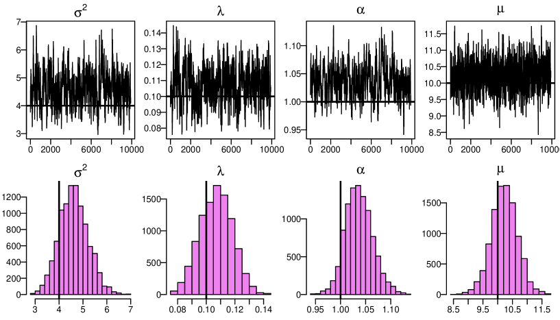
Figure 2: MCMC trace plots and histograms for the parameters. Results are based on simulated data on a $128\times 128$ lattice with 10% missing data in a disk shape. The true parameter values are $\sigma^{2}=4$, $\lambda=0.1$, $\alpha=1$ and $\mu=10$.

The results from the MCMC algorithm are reported in Table 3 and Figures 2–3. All results are based on the Vecchia preconditioner with prediction sets of size 4 and conditioning sets of size 52, with a PCG tolerance of $\epsilon=10^{-5}$. Calculations are implemented in C on an Intel Xeon 2.8 GHz processor with 22 GB of RAM on a Mac OS X operating system. Fast Fourier transforms are implemented with the FFTW package (Frigo and Johnson, 1998).

Figures 2 and 3 show the results from the MCMC analysis of simulated data on a $128\times 128$ lattice with 10% missing values in a disk-shaped region. In total, there are 14,743 observations. The MCMC described above was run for 10,000 iterations after a burn-in period of 1000. Figure 2 shows posterior trace plots and histograms for the parameters. The trace plots are stable, indicating no clear violations of stationarity. The histograms are all unimodal and fairly symmetric. All of the histograms contain the true parameter values, and all of the 95% posterior intervals (not shown) contain the true parameter values. This indicates that the algorithm is providing accurate samples from the posterior distribution.

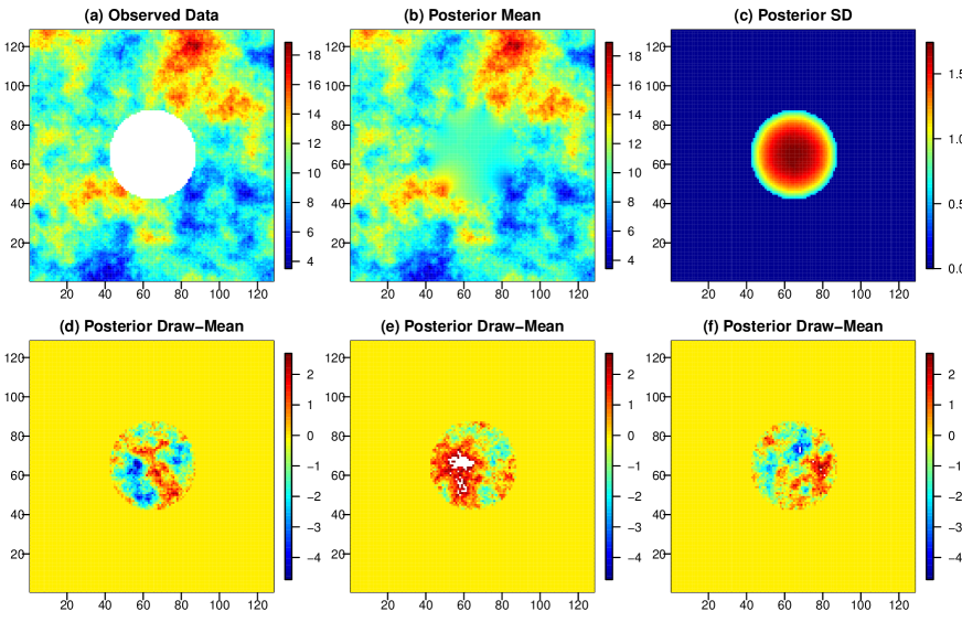
Figure 3: MCMC posterior summaries of the random field for simulated data on a $128\times 128$ lattice with 10% missing data in a disk shape. (a) observed data $Z(\mathbf{s})$. (b)-(c) posterior mean and standard deviation for $Z(\mathbf{s})$. (d)-(f) posterior draws minus the posterior mean for $Z(\mathbf{s})$.

Figure 3 summarizes the posterior distribution of the spatial field. Panels (a) shows the observed data $Z(\mathbf{s})$, (b) and (c) show the posterior mean and standard deviation for the field, and panels (d)-(f) show three posterior draws minus the posterior mean. Note that the posterior mean agrees with the observed data at the observation locations, and converges to the unconditional mean ($\hat{\mu}\approx 10$) near the center of the domain. In addition, there is no posterior uncertainty for $Z(\mathbf{s})$ at the observation locations, and the posterior standard deviation converges to the unconditional SD ($\hat{\sigma}\approx 2$) near the center of the domain. Panels (d)-(f) illustrate the sample-to-sample variation in the posterior field; the plots illustrate the correlation length scales and reiterate that the uncertainty is highest in the center of the domain.

Next, we study the behavior of the MCMC algorithm for different lattice sizes and different missingness patterns. As stated earlier, we consider increasingly dense lattices of size $n_{1}\times n_{1}$ with $n_{1}=$ 32, 64, 128, 256 and 512, with corresponding embedding lattices of size $3n_{1}\times 3n_{1}$. We consider three designs: complete lattice, 10% missing at random, and 10% missing disk. The results described below are based on 2000 MCMC iterations after a burn-in period of 500. The true parameter values, choice of $r$, and proposal distribution, are the same as above.

$n_{1}$	$n$	$\sigma^{2}$	$\lambda$	$\alpha$	$\mu$	Iter	Time
Complete Lattice
32	1024	4.25 (0.92)	0.094 (0.024)	1.057 (0.057)	9.48 (0.40)	5	1
64	4096	3.10 (0.69)	0.090 (0.026)	0.942 (0.027)	9.84 (0.34)	8	3
128	16384	4.38 (0.47)	0.103 (0.010)	1.030 (0.022)	10.35 (0.40)	13	23
256	65536	4.10 (0.27)	0.100 (0.004)	1.012 (0.021)	9.89 (0.36)	22	167
512	262144	4.05 (0.09)	0.098 (0.002)	1.011 (0.010)	9.66 (0.36)	38	1248
Missing at Random (10%)
32	922	3.94 (0.88)	0.084 (0.025)	1.104 (0.074)	9.29 (0.37)	24	1
64	3675	2.97 (0.61)	0.081 (0.019)	0.963 (0.028)	9.87 (0.30)	28	8
128	14707	4.37 (0.51)	0.104 (0.010)	1.024 (0.023)	10.24 (0.41)	46	60
256	58912	4.06 (0.27)	0.101 (0.004)	1.006 (0.021)	9.88 (0.38)	67	429
512	235730	4.02 (0.09)	0.098 (0.002)	1.008 (0.012)	9.61 (0.38)	99	2985
Missing Disk (10%)
32	923	4.29 (0.98)	0.092 (0.025)	1.089 (0.067)	9.32 (0.46)	20	1
64	3675	2.86 (0.55)	0.084 (0.020)	0.937 (0.029)	9.86 (0.33)	40	9
128	14743	4.49 (0.58)	0.105 (0.011)	1.034 (0.028)	10.26 (0.38)	74	87
256	58979	4.04 (0.22)	0.101 (0.004)	1.003 (0.018)	9.85 (0.41)	130	753
512	235923	3.99 (0.09)	0.099 (0.003)	1.005 (0.013)	9.66 (0.42)	257	7470

Table 1: MCMC results, power exponential covariance with nugget, for different lattice sizes and sampling designs. The table shows the lattice size ($n_{1}=n_{2}$), number of observations $n$, posterior means (standard deviations) for the unknown parameters, average number of PCG iterations per conditional simulation, and the computational run time (in minutes) for 2500 MCMC iterations. The true parameter values are $\sigma^{2}=4,\lambda=0.1,\alpha=1$ and $\mu=10$. Each row corresponds to one simulated dataset. The PCG tolerance is $\epsilon=10^{-5}$.

Table 3 reports the parameter estimates, number of PCG iterations, and computational run times for the MCMC results. For each lattice size and missingness pattern, we report the posterior means and standard deviations for the unknown parameters, the average number of PCG iterations per conditional simulation, and total run time in minutes. There are a number of points to note. First, the posterior means are fairly close to the true values, with the 95% posterior intervals (not shown) containing the true values for all parameters in all examples. Second, notice that the posterior standard deviation decreases as $n$ increases for all parameters except $\mu$. The latter is expected under fixed-domain asymptotics (Stein, 1999), since the degree of ‘learning’ about the mean is limited by the size of the domain rather than the lattice size.

Third, the average number of PCG iterations depends on lattice size and missingness pattern. In particular, the number of iterations increases with the lattice size. For example, for complete lattices, the average number of PCG iterations increases from 5 for a $32\times 32$ grid to 38 for a $512\times 512$ grid. Similar increases occur for the other two sampling designs. In addition, complete lattice designs require fewer PCG iterations than incomplete lattices. For example, for $128\times 128$ lattices, the complete design requires 13 iterations, missing at random requires 46 iterations, and missing disk requires 74 iterations. Presumably, this occurs because the Vecchia preconditioner provides a better approximation to the precision matrix for complete lattices than for incomplete lattices. To quantify these relationships, we fit multiple regressions of the number of PCG iterations against grid size and sampling design. Based on the fitted models (not shown), we conclude that the number of PCG iterations increases like the square root of the number of lattice points, i.e., $I(N)=O(N^{1/2})$.

Finally, note that the MCMC run times are roughly proportional to the number of PCG iterations. For the complete lattice design, 2500 iterations of the MCMC algorithm requires about one minute for a $32\times 32$ lattice, three minutes for $64\times 64$ lattice, 23 minutes for a $128\times 128$ lattice, and about 2.8 hours for a $256\times 256$ lattice. The run times for $n_{1}=128$ and $n_{1}=256$ are impressive, considering that no other ‘exact’ Bayesian methods exist for datasets of this size.

4.1.2 Maximum Likelihood Analysis

For maximum likelihood analysis, we use the EM algorithm from Section 3.2 with modifications to improve computational efficiency. In particular, the form of the likelihood allows us to use profile methods in the M-step. Under the model in Section 4.1, the conditional expectation is

$$Q(\mu,\sigma^{2},\mbox{\boldmath$\theta$}|\mathbf{\Theta}^{t})=-\frac{N}{2}\log\sigma^{2}-\frac{1}{2}\log|\mathbf{C}(\mbox{\boldmath$\theta$})|-\frac{1}{2\sigma^{2}}E\left[(\mathbf{Z}-\mu\mathbf{1})^{\prime}\mathbf{C}(\mbox{\boldmath$\theta$})^{-1}(\mathbf{Z}-\mu\mathbf{1})|\mathbf{Z}_{o},\mathbf{\Theta}^{t}\right].$$ (15)

Using equations (8)-(9) with $\mbox{\boldmath$\mu$}=\mu\mathbf{1}$ and $\mathbf{C}=\sigma^{2}\mathbf{C}(\mbox{\boldmath$\theta$})$, and differentiating with respect to $\mu$ and $\sigma^{2}$, we find that (15) is maximized at

$$\hat{\mu}(\mbox{\boldmath$\theta$}) = \frac{\mathbf{1}^{\prime}\mathbf{C}(\mbox{\boldmath$\theta$})^{-1}\widetilde{}\mbox{\boldmath$\mu$}}{\mathbf{1}^{\prime}\mathbf{C}(\mbox{\boldmath$\theta$})^{-1}\mathbf{1}}=\frac{\mathbf{1}^{\prime}\widetilde{}\mbox{\boldmath$\mu$}}{N},$$ (16)

$$\hat{\sigma}^{2}(\mbox{\boldmath$\theta$}) = E\left[S^{2}(\mbox{\boldmath$\theta$})|\mathbf{Z}_{o},\mathbf{\Theta}^{t}\right]/N,$$ (17)

$$\hat{}\mbox{\boldmath$\theta$} = \arg\max_{\mbox{\boldmath$\theta$}}Q_{p}(\mbox{\boldmath$\theta$}|\mathbf{\Theta}^{t}),$$ (18)

where $\widetilde{}\mbox{\boldmath$\mu$}=E(\mathbf{Z}|\mathbf{Z}_{o},\mathbf{\Theta}^{t})$ is the conditional mean, $S^{2}(\mbox{\boldmath$\theta$})=(\mathbf{Z}-\hat{\mu}\mathbf{1})^{\prime}\mathbf{C}(\mbox{\boldmath$\theta$})^{-1}(\mathbf{Z}-\hat{\mu}\mathbf{1})$ is the generalized sum of squares, and $Q_{p}(\mbox{\boldmath$\theta$}|\mathbf{\Theta}^{t})$ is the profile function for $\theta$ obtained by substituting $\hat{\mu}(\mbox{\boldmath$\theta$})$ and $\hat{\sigma}^{2}(\mbox{\boldmath$\theta$})$ into (15). Note that $\hat{\mu}(\mbox{\boldmath$\theta$})$ does not depend on $\theta$ because $\mathbf{C}(\mbox{\boldmath$\theta$})^{-1}$ is BCCB, so $\hat{\mu}$ can be computed independently of the other parameters. The profile function for $\theta$ is

$$Q_{p}(\mbox{\boldmath$\theta$}|\mathbf{\Theta}^{t})=-\frac{N}{2}\log\hat{\sigma}^{2}(\mbox{\boldmath$\theta$})-\frac{1}{2}\log|\mathbf{C}(\mbox{\boldmath$\theta$})|.$$ (19)

This function is maximized to obtain the estimate $\hat{}\mbox{\boldmath$\theta$}$. The estimate for $\sigma^{2}$ is then obtained as $\hat{\sigma}^{2}(\hat{}\mbox{\boldmath$\theta$})$ in (17). However, as noted before, the conditional expectation of $S^{2}(\mbox{\boldmath$\theta$})$ in (17) is computationally intractible for large datasets, so we approximate it using Monte Carlo methods. The Monte Carlo estimate for the expected sum of squares is

$$\hat{S}^{2}(\mbox{\boldmath$\theta$})=\frac{1}{M}\sum_{i=1}^{M}S^{2}_{i}(\mbox{\boldmath$\theta$})$$ (20)

where $S^{2}_{i}(\mbox{\boldmath$\theta$})=(\mathbf{Z}^{(i)}-\hat{\mu}\mathbf{1})^{\prime}\mathbf{C}(\mbox{\boldmath$\theta$})^{-1}(\mathbf{Z}^{(i)}-\hat{\mu}\mathbf{1})$, and $\mathbf{Z}^{(i)}\sim p(\mathbf{Z}\,|\,\mathbf{Z}_{o},\mathbf{\Theta}^{t})$, for $i=1,\ldots,M$ are conditional simulations of the complete data generated using the current parameter value $\mathbf{\Theta}^{t}$. We then substitute $\hat{S}^{2}(\mbox{\boldmath$\theta$})$ for $E\left[S^{2}(\mbox{\boldmath$\theta$})|\mathbf{Z}_{o},\mathbf{\Theta}^{t}\right]$ in (17) and (19) to obtain an approximate profile function, $\widehat{Q}_{p}(\mbox{\boldmath$\theta$}|\mathbf{\Theta}^{t})$. This function is then maximized to obtain the estimates $\hat{}\mbox{\boldmath$\theta$}$ and $\hat{\sigma}^{2}=\hat{\sigma}^{2}(\hat{}\mbox{\boldmath$\theta$})$. Since $\widehat{Q}_{p}(\mbox{\boldmath$\theta$}|\mathbf{\Theta}^{t})$ cannot be maximized analytically, we use numerical methods to obtain $\hat{}\mbox{\boldmath$\theta$}$.

We illustrate the maximum likelihood estimation procedure by generating 50 datasets on a $32\times 32$ square lattice, assuming a complete lattice design and two incomplete designs (missing at random and missing disk) with three missingness probabilities (10%, 25%, 50%). We assume an exponential covariance with no microscale variation by fixing $\alpha=1$ and $c=0$. The true values for the unknown parameters are $\sigma^{2}=2$, $\lambda=0.141$ and $\mu=0$. The exponential model is used in this example because it has a closed-form spectral density, which is needed for the two competing spectral methods described below.

For the EM algorithm, we use the approach described above with a Monte Carlo sample size of $M=400$, using the Vecchia preconditioner and a PCG tolerance of $\epsilon=10^{-5}$ as in Section 4.1.1. For comparison, we also implement two approximate maximum likelihood methods: the composite likelihood approach of Vecchia (1988) and Stein et al. (2004), using prediction sets of size 4 and conditioning sets of size 52; and the spectral approximations of Whittle (1954) and Fuentes (2007) for complete and incomplete lattices, respectively. Note that we also considered other approximate likelihood methods (e.g., covariance tapering), but the composite likelihood and spectral methods were easier to implement and generally gave more accurate results, so the other results are not reported here.

		$\sigma^{2}$					$\lambda$					$\mu$
Design		$R^{*}$	$R_{1}$	$R_{2}$	$R_{3}$		$R^{*}$	$R_{1}$	$R_{2}$	$R_{3}$		$R^{*}$	$R_{1}$	$R_{2}$	$R_{3}$
Complete		450	26	45	387		35	3	4	33		550	2	22	237
Random 10%		446	31	58	596		47	3	6	92		545	2	54	231
Random 25%		450	80	75	626		50	8	8	127		556	3	93	220
Random 50%		457	25	132	552		49	2	13	147		558	3	156	227
Disk 10%		442	26	268	370		47	3	25	40		554	3	393	212
Disk 25%		466	24	207	385		48	2	21	51		557	3	314	174
Disk 50%		491	60	317	351		47	6	31	65		554	4	399	163

Table 2: Maximum likelihood estimation, exponential covariance model, 32 $\times$ 32 lattice, different sampling designs, based on 50 simulated datasets. We report the RMSE ($R^{*}$) and RMSD ($R_{k}$) for three competing methods: $R_{1}=$ EM algorithm; $R_{2}=$ composite likelihood; $R_{3}=$ spectral approximation. Here, $R^{*}=(\frac{1}{50}\sum_{r=1}^{50}(\hat{\theta}_{r}-\theta)^{2})^{1/2}$ and $R_{k}=(\frac{1}{50}\sum_{r=1}^{50}(\hat{\theta}_{k,r}-\hat{\theta}_{r})^{2})^{1/2}$, where $\theta$ is the true parameter value, $\hat{\theta}_{r}$ is the exact MLE, and $\hat{\theta}_{k,r}$ is the approximate MLE for method $k$. True parameter values are $\sigma^{2}=2$, $\lambda=0.141$, $\mu=0$. All values are multiplied by 1000.

Table 2 shows the root mean squared differences (RMSD) for each of the estimation methods: EM algorithm, composite likelihood, and spectral approximation. For each unknown parameter $\theta\in\{\sigma^{2},\lambda,\mu\}$, and each estimation method $k=1,2,3$, we define

$$\mbox{RMSD}_{k}=\left(\frac{1}{50}\sum_{r=1}^{50}(\hat{\theta}_{k,r}-\hat{\theta}_{r})^{2}\right)^{1/2},$$

where $\hat{\theta}_{k,r}$ denotes the approximate ML estimate for method $k$, and $\hat{\theta}_{r}$ denotes the exact ML estimate, for each replicate $r=1,2,\ldots,50$. The exact MLE can be computed due to the small sample size in this example ($n\leq 1024$). Note that our definition of RMSD depends on the difference between the approximate MLE and the true MLE, rather than the true parameter. This allows us to focus on the approximation error of the estimate (i.e., an RMSD of zero corresponds to an estimate with no approximation error.) For comparison, we also compute the root mean squared error for the exact MLE, which is defined as $\mbox{RMSE}=(\frac{1}{50}\sum_{r=1}^{50}(\hat{\theta}_{r}-\theta)^{2})^{1/2}$, where $\theta$ is the true parameter value. For all methods, we use a modified Nelder-Mead simplex algorithm for numerical maximization.

Overall, our method outperforms the other two methods for all spatial designs and parameters, except one. First, note that the spectral methods are highly inaccurate, with RMSDs that are often 100 times larger than our approach. The large RMSD for the spectral approach is largely due to a strong negative bias for the sill and range parameters (not shown). This bias has been well documented (Guyon, 1982), and many improvements have been proposed, including data tapering (Dalhaus and Künsch, 1987). However, we repeated the analysis using data tapering and the results did not improve much. Second, composite likelihood is more accurate than the spectral approximation, but worse than our approach. Its performance degrades as the proportion of missing data increases. It performs especially poorly for the missing-disk design. This indicates that the local approximation for composite likelihood breaks down near the boundaries of large contiguous blocks of missing data. The composite likelihood results could possibly be improved by including some distant neighbors in the conditioning set (Stein et al., 2004); however, it is not obvious how to determine a neighborhood scheme that would work well for all designs.

For the sill and range parameters, $\sigma^{2}$ and $\lambda$ the RMSDs for our approach are about 30% lower for complete lattice, and 50–90% lower for the incomplete lattices. For the mean parameter $\mu$, the results are particularly striking: our estimates are substantially more accurate than the other two approaches, with our RMSDs 90–99% lower than the competing methods.

4.2 Application to Satellite Sea Surface Temperatures

For a real application, we consider a composite TMI satellite image of sea surface temperatures over the Pacific Ocean during the month of March 1998, shown in Figure 4(a). This dataset was also analyzed by Fuentes (2007), who used spectral methods to fit a stationary Gaussian process to the data for maximum likelihood estimation. The observations represent monthly averages of sea surface temperatures in the Pacific Ocean on a 120 $\times$ 80 grid; the process is undefined over land regions in South and Central America and the Galapagos Islands. The process appears to be somewhat nonstationary, but for illustration, we treat it as a stationary process with unknown mean and Matérn covariance function with nugget effect. The percentage of missing data is about 4%, and the total number of observations is $n=9203$.

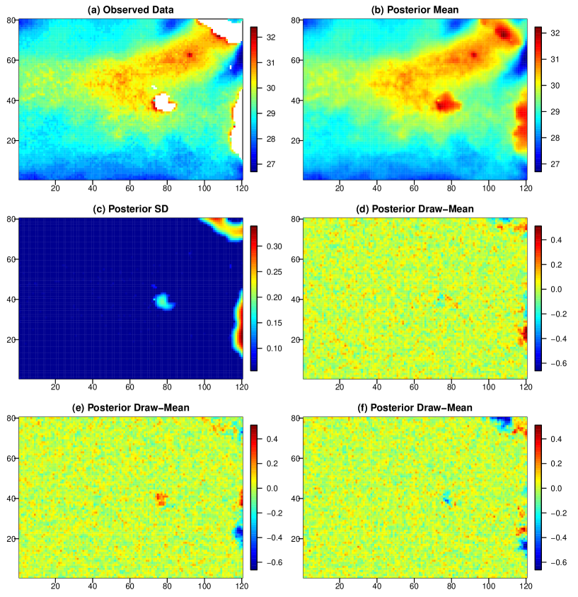
Figure 4: TMI satellite data. (a) Observed data $Y(\mathbf{s})$. (b)-(c) Posterior mean and standard deviation for $Z(\mathbf{s})$. (d)-(f) Posterior draws minus the posterior mean for $Z(\mathbf{s})$.

To compare our results with Fuentes (2007), we assume that the observed data $Y(\mathbf{s})$ can be written as $Y(\mathbf{s})=Z(\mathbf{s})+\varepsilon(\mathbf{s})$, where $\varepsilon(\mathbf{s})$ is a white noise process with mean zero and variance $\tau^{2}$, and $Z(\mathbf{s})$ is a stationary, isotropic process with Matérn covariance function (Stein, 1999), $C(h)=\sigma^{2}\varphi(h)$, where

$$\varphi(h)=\frac{1}{2^{\nu-1}\Gamma(\nu)}\left(\frac{h}{\lambda}\right)^{\nu}\mathcal{K}_{\nu}\left(\frac{h}{\lambda}\right),$$ (21)

where $\sigma^{2}$ and $\lambda$ are the sill and range parameters, $\nu>0$ is the smoothness parameter, $\mathcal{K}_{\nu}$ is a modified Bessel function of the third kind of order $\nu$ (see Abramowitz and Stegun, 1964, sec. 9) and $\tau^{2}$ is the nugget effect. Note that the model in Fuentes (2007) also included two anisotropy parameters; however, both parameters were found to be insignificant, implying that the process is isotropic. We implement the Bayesian MCMC approach described in Sections 3.1 and 4.1.1 to estimate the parameters $\mu,\sigma^{2}$ and $\mbox{\boldmath$\theta$}=(\lambda,\nu,c)$ where $c=\tau^{2}/\sigma^{2}$ is the noise-to-signal ratio. We assume the following independent prior distributions: $\pi(\mu,\sigma^{2})\propto\sigma^{-2}$, $\pi(\lambda)\propto 0.5(1+0.5\lambda)^{-2}$, $\nu\sim\mathcal{U}(0,50)$ and $c\sim\mathcal{U}(0,10)$.

Because of the non-square lattice, our embedding approach requires slight modification. We embed the original $120\times 80$ lattice in a square lattice of size $320\times 320$. We define the maximum distance in the original domain, $\sqrt{120^{2}+80^{2}}\approx 144.2$ pixels, to be 1 distance unit. We then apply the embedding approach as in Section 4.1 with a radius of $r=1.5/\sqrt{2}\approx 1.06$. This implies that the minimum size for the embedding lattice is $2r\cdot 144.2\approx 305.7$, which is then rounded up to the next highly composite integer of 320. Note that this choice of radius and embedding lattice led to a small number of negative eigenvalues in the sampler. We discarded these parameter draws, under the prior assumption that the parameters are constrained to values that yield non-negative definite embeddings. The MCMC algorithm described in Section 4.1.1 was run for 65,000 iterations after a burn-in period of 35,000.

Figure 5: TMI satellite data. Posterior histograms and pairs plots for the Matérn covariance parameters. Note that $\lambda$ are in units of km, which are obtained by multiplying their original distance units by (144.2 pixels/distance unit) $\cdot$ (25 km/pixel) = 3605 km/distance unit.

Figure 4 shows the observed data $Y(\mathbf{s})$, and the posterior mean, standard deviation and three posterior draws of the unobserved spatial field, $Z(\mathbf{s})$. Since the nugget effect is relatively small, the posterior mean for the unobserved field $Z(\mathbf{s})$ closely matches the observed data $Y(\mathbf{s})$ where available, but is much smoother. The posterior standard deviation and draws illustrate the posterior uncertainty for $Z(\mathbf{s})$, which is small except over the land regions. Figure 5 shows the posterior histograms and scatterplots for the parameters. Note that the posterior distributions are all unimodal and fairly symmetric. There are dependencies between the parameters, most notably a strong positive correlation between the smoothness parameter $\nu$ and the nugget effect $\tau^{2}$.

Table 3 compares the posterior means and standard deviations for the parameters from our MCMC approach with the spectral ML estimates and standard errors reported in Fuentes (2007). For comparison we also calculate the exact maximum likelihood estimates and their asymptotic standard errors, which are just barely computable for a sample size of $n=9203$. Note that our results differ substantially from the spectral method: our estimates are $\hat{\sigma}^{2}=1.54$, $\hat{\lambda}=953$ km, $\hat{\nu}=0.72$ and $\hat{\tau}^{2}=0.006$, while those from Fuentes (2007) are $\hat{\sigma}^{2}=0.57$, $\hat{\lambda}=312$ km, $\hat{\nu}=1.00$ and $\hat{\tau}^{2}=0.001$. However, the estimates of $\sigma^{2}/\lambda$, which relates to the fine scale variation of the process, are similar. The standard errors are also quite different for the two approaches, in particular for $\sigma^{2}$ (0.40 vs. 0.02) and $\nu$ (0.04 vs. 1.20). On the other hand, our estimates and standard errors agree closely with the exact ML values for all parameters. This is quite reassuring. As a final comparison, we compute the exact loglikelihood values for the three sets of estimates. The loglikelikehood for the spectral estimates is -2077, while the MCMC estimates and exact MLEs have nearly identical loglikelihoods of 5528, an improvement of 7605 points over the spectral approach.

Method	$\sigma^{2}$	$\lambda$	$\sigma^{2}/\lambda$	$\nu$	$\tau^{2}$	Loglike
Spectral MLE	0.57 (0.02)	312 ( 70)	.0018 (——-)	1.00 (1.20)	.0010 (.0020)	-2077.11
MCMC Bayes	1.54 (0.40)	953 (215)	.0016 (.0003)	0.72 (0.04)	.0066 (.0005)	5528.13
Exact MLE	1.45 (0.52)	911 (312)	.0016 (——-)	0.72 (0.04)	.0066 (.0006)	5528.19

Table 3: TMI satellite data. Comparison of parameter estimates (standard errors) for the spectral MLE results reported in Fuentes (2007), from our Bayesian MCMC approach, and the exact MLEs. No standard errors are available for $\sigma^{2}/\lambda$ for the spectral and exact MLEs. The last column shows the exact log-likelihood values for each set of estimates.

5 Conclusions

In this paper, we have proposed a new approach for Bayesian and maximum likelihood parameter estimation for stationary Gaussian processes observed on a large, possibly incomplete, lattice. We find that the method is feasible for large datasets (lattices of up to size $512\times 512$), it allows for missing data or lattices with non-rectangular boundaries, and it provides accurate inference for the parameters and missing values. We propose an MCMC algorithm for Bayesian inference and a Monte Carlo EM algorithm for maximum likelihood estimation. The method requires the choice of a preconditioner matrix for the PCG algorithm. We have developed a number of new preconditioners, and have found that two work quite well: the observed block of the complete inverse covariance matrix, and an incomplete Cholesky preconditioner based on the composite likelihood methods of Vecchia (1988) and Stein et al. (2004). The latter performs best overall in the examples we considered.

The proposed algorithms are widely applicable and conceptually simple, requiring iteration between updating the missing data and the parameters. The main challenges in using the method are: (1) selection of a periodic covariance function and an embedding lattice that ensures non-negative definiteness of the $\mathbf{C}$ matrix; (2) choosing a fast preconditioner that performs well under different parameter values, lattice sizes, and missingness patterns; and (3) a need for computational code to implement the method. With regards to the latter, we have developed efficient C code for the method, which we plan to make available upon publication of this paper.

Possible extensions of this work include estimation of nonstationary processes, non-Gaussian processes, multivariate spatial processes, and spatio-temporal models. We have implemented the approach for anisotropic processes; however, the results are not reported here for space reasons. We note that another estimation approach using circulant embedding is a Gibbs Sampler as proposed by Kozintsev and Kedem (2000) for clipped Gaussian fields. For this approach, the unobserved values on the embedding lattice are generated one location at a time. This is computationally expensive, requiring $O(N^{2})$ operations, where $N$ is the number of locations, which is infeasible when $N$ is large. Our proposed approach based on conditional simulations uses simultaneous updating, and thus should provide a more efficient approach to these problems. Finally, we also plan to explore the use of parallel methods to further improve efficiency of the algorithm.

Appendix A: BCCB Matrices

Let $\mathbf{C}$ be a $N\times N$ block circulant matrix with circulant blocks (BCCB). Then $\mathbf{C}=\mathbf{F}\mathbf{\Lambda}\mathbf{F}^{*}$, where $\mathbf{F}$ is the $2-$dimensional forward Fourier transform (FFT) matrix, $\mathbf{F}^{*}$ is the inverse FFT matrix, and $\mathbf{\Lambda}=\mbox{diag}(\mbox{\boldmath$\lambda$})$ is the matrix of eigenvalues, where $\mbox{\boldmath$\lambda$}=(\lambda_{1},\ldots,\lambda_{N})$. These matrices have a number of computational advantages, namely that their eigenvalues, matrix-vector multiplications, and quadratic forms can all be computed in $O(N\log N)$ operations using the FFT. We summarize these operations below.

1. Eigenvalues: $\mbox{\boldmath$\lambda$}=\mathbf{F}\mathbf{c}$ (where $\mathbf{c}$ is the first column of $\mathbf{C}$).

2. Matrix inverse: $\mathbf{C}^{-1}=\mathbf{F}\mathbf{\Lambda}^{-1}\mathbf{F}^{*}$.

3. Matrix-vector multiplication: $\mathbf{C}\mathbf{x}=\mathbf{F}\mathbf{\Lambda}\mathbf{F}^{*}\mathbf{x}$.

4. Cholesky-vector multiplication: $\mathbf{L}\mathbf{x}=\mathbf{\Lambda}^{1/2}\mathbf{F}^{*}\mathbf{x}$ (where $\mathbf{C}=\mathbf{L}\mathbf{L}^{\prime}$).

5. Quadratic form: $\mathbf{x}^{\prime}\mathbf{C}\mathbf{x}=(\mathbf{\Lambda}^{1/2}\mathbf{F}^{*}\mathbf{x})^{\prime}(\mathbf{\Lambda}^{1/2}\mathbf{F}^{*}\mathbf{x})=\mathbf{z}^{\prime}\mathbf{z}$.

Multiplications of the form $\mathbf{F}\mathbf{x}$ and $\mathbf{F}^{*}\mathbf{x}$ are computed using the $2-$dimensional forward and backward FFT’s, respectively, which require $O(N\log N)$ operations each. Matrix-vector multiplications involving the diagonal matrix $\mathbf{\Lambda}$ are computed by vector-vector multiplications, requiring $O(N)$ calculations. Thus, all of the above calculations require $O(N\log N)$ operations.

Appendix B: Preconditioned Conjugate Gradient

The preconditioned conjugate gradient (PCG) algorithm is an iterative method to solve the system, $\mathbf{A}\mathbf{x}=\mathbf{b}$, where $\mathbf{A}$ is an $n\times n$ symmetric positive-definite matrix and $\mathbf{b}\in\mathbb{R}^{n}$ is known. The PCG method actually solves the equivalent system $\mathbf{M}^{-1}\mathbf{A}\mathbf{x}=\mathbf{M}^{-1}\mathbf{b}$, where $\mathbf{M}^{-1}$ is an $n\times n$ preconditioner matrix chosen such that $\mathbf{M}^{-1}\mathbf{A}$ is better conditioned than $\mathbf{A}$. The algorithm updates three vectors in $\mathbb{R}^{n}$: the solution $\mathbf{x}$, the residual $\mathbf{r}$, and the search direction $\mathbf{p}$. The initial solution is defined as $\mathbf{x}_{0}=\mathbf{M}^{-1}\mathbf{b}$; the initial residual and direction are defined as $\mathbf{r}_{0}=\mathbf{b}-\mathbf{A}\mathbf{x}_{0}$ and $\mathbf{p}_{0}=\mathbf{M}^{-1}\mathbf{r}_{0}$. The algorithm then proceeds as follows for $k=0,1,2,\ldots$

$$\alpha_{k+1} = (\mathbf{r}_{k}^{\prime}\mathbf{M}^{-1}\mathbf{r}_{k})/(\mathbf{p}_{k}^{\prime}\mathbf{A}\mathbf{p}_{k})$$

$$\mathbf{x}_{k+1} = \mathbf{x}_{k}+\alpha_{k+1}\mathbf{p}_{k}$$

$$\mathbf{r}_{k+1} = \mathbf{r}_{k}-\alpha_{k+1}\mathbf{A}\mathbf{p}_{k}$$

$$\beta_{k+1} = (\mathbf{r}_{k+1}^{\prime}\mathbf{M}^{-1}\mathbf{r}_{k+1})/(\mathbf{r}_{k}^{\prime}\mathbf{M}^{-1}\mathbf{r}_{k})$$

$$\mathbf{p}_{k+1} = \mathbf{M}^{-1}\mathbf{r}_{k+1}+\beta_{k+1}\mathbf{p}_{k}$$

The algorithm is terminated at the iteration $k=I$ when the residual is less than a specified relative error, i.e., when $|\mathbf{r}_{k}|/|\mathbf{r}_{0}|<\epsilon$, where $\epsilon$ is the specified tolerance.

Appendix C: Vecchia Preconditioner

We define the preconditioner $\mathbf{M}^{-1}$ used in the examples. The goal is to solve the system $\mathbf{\Sigma}\mathbf{x}=\mathbf{b}$, where $\mathbf{\Sigma}$ is the $n\times n$ covariance matrix for a stationary process on a lattice, and $\mathbf{b}$ is a known vector. We define $\mathbf{M}^{-1}$ as the inverse covariance matrix implied by the composite likelihood methods of Vecchia (1988) and Stein, Chi and Welty (2004). Let $\mathbf{Z}$ be an $n\times 1$ random vector with distribution $\mathcal{N}(\mathbf{Z}|\mathbf{0},\mathbf{\Sigma})$. For composite likelihood methods (see Varin, Reid and Firth, 2011), the observations are ordered into $q$ blocks, and the likelihood is written as a product of $q$ conditional densities, $p(\mathbf{A}_{j}\mathbf{Z}|\mathbf{B}_{j}\mathbf{Z}),j=1,\ldots,q$, where $\mathbf{A}_{j}$ and $\mathbf{B}_{j}$ are $n_{j}\times n$ and $m_{j}\times n$ matrices of zeros and ones defining the prediction and conditioning sets for block $j$. The conditional distributions have the form $\mathcal{N}(\mathbf{A}_{j}\mathbf{Z}|\mathbf{K}_{j}\mathbf{B}_{j}\mathbf{Z},\mathbf{V}_{j})$, where

$$\mathbf{K}_{j} = \mathbf{A}_{j}\mathbf{\Sigma}\mathbf{B}_{j}^{\prime}(\mathbf{B}_{j}\mathbf{\Sigma}\mathbf{B}_{j}^{\prime})^{-1}$$

$$\mathbf{V}_{j} = \mathbf{A}_{j}\mathbf{\Sigma}\mathbf{A}_{j}^{\prime}-\mathbf{A}_{j}\mathbf{\Sigma}\mathbf{B}_{j}^{\prime}(\mathbf{B}_{j}\mathbf{\Sigma}\mathbf{B}_{j}^{\prime})^{-1}\mathbf{B}_{j}\mathbf{\Sigma}\mathbf{A}_{j}^{\prime}$$

are matrices of size $n_{j}\times m_{j}$ and $n_{j}\times n_{j}$, respectively. Let $\mathbf{L}_{j}=\mathbf{A}_{j}-\mathbf{K}_{j}\mathbf{B}_{j}$ be the $n_{j}\times n$ matrix such that $\mathbf{L}_{j}\mathbf{Z}$ are the errors in the regression of $\mathbf{A}_{j}\mathbf{Z}$ on $\mathbf{B}_{j}\mathbf{Z}$. Then $\mathbf{L}_{j}\mathbf{Z}\sim\mathcal{N}(\mathbf{0},\mathbf{V}_{j})$ independently, and the approximate loglikelihood can be written as (ignoring additive constants)

$$\log p(\mathbf{Z})=\sum_{j=1}^{q}\left(-\frac{1}{2}\log|\mathbf{V}_{j}|-\frac{1}{2}\mathbf{Z}^{\prime}\mathbf{L}_{j}^{\prime}\mathbf{V}_{j}^{-1}\mathbf{L}_{j}\mathbf{Z}\right).$$

This is the loglikelihood for the multivariate normal density $\mathcal{N}(\mathbf{Z}|\mathbf{0},\mathbf{V})$, where

$$\mathbf{V}^{-1}\,=\,\sum_{j=1}^{q}\mathbf{L}_{j}^{\prime}\mathbf{V}_{j}^{-1}\mathbf{L}_{j}.$$

This suggests that $\mathbf{V}^{-1}\approx\mathbf{\Sigma}^{-1}$, and therefore we choose $\mathbf{V}^{-1}$ as the preconditioner. This matrix is sparse, and can be fully represented in terms of the smaller matrices $\mathbf{K}_{j}$ and $\mathbf{V}_{j}$. Many of these matrices are identical due to the stationarity assumption and the lattice domain, so we only need to compute and store the unique $\mathbf{K}_{j}$ and $\mathbf{V}_{j}$. In concise form, we can write $\mathbf{V}^{-1}=\mathbf{L}^{\prime}\mathbf{D}\mathbf{L}$, where $\mathbf{D}=\mbox{block diag}(\mathbf{V}_{1}^{-1},\ldots,\mathbf{V}_{q}^{-1})$ and $\mathbf{L}=[\mathbf{L}_{1}^{\prime}~{}\mathbf{L}_{2}^{\prime}~{}\cdots~{}\mathbf{L}_{q}^{\prime}]^{\prime}$ are sparse $n\times n$ matrices. To perform multiplications $\mathbf{w}=\mathbf{V}^{-1}\mathbf{x}$, we first compute $\mathbf{u}=\mathbf{D}\mathbf{L}\mathbf{x}$, and then $\mathbf{w}=\mathbf{L}^{\prime}\mathbf{u}$, which can be computed efficiently by summing over the blocks as follows:

$$\mathbf{u}=\mathbf{D}\mathbf{L}\mathbf{x}\,=\,\sum_{j=1}^{q}\mathbf{V}_{j}^{-1}\mathbf{L}_{j}\mathbf{x},$$

$$\mathbf{w}=\mathbf{L}^{\prime}\mathbf{u}\,=\,\sum_{j=1}^{q}\mathbf{L}_{j}^{\prime}\mathbf{u}.$$

References

- Abramowitz and Stegun (1964) Abramowitz, M. and Stegun, I. A. (1964) Handbook of Mathematical Functions. New York: Dover.
- Agarwal and Gelfand (2005) Agarwal, D. K. and Gelfand, A. E. (2005) Slice sampling with application to spatial data. Statistics and Computing, 15, 61–69.
- Banerjee et al. (2008) Banerjee, S., Gelfand, A., Finley, A. and Sang, H. (2008) Gaussian predictive process models for large spatial data sets. Journal of the Royal Statistical Society, Series B, 70, 825–848.
- Berger et al. (2001) Berger, J. O., De Oliveira, V. and Sansó, B. (2001) Objective Bayesian analysis of spatially correlated data. Journal of the American Statistical Association, 96, 1361–1374.
- Chilès and Delfiner (2012) Chilès, J.-P. and Delfiner, P. (2012) Geostatistics: Modeling Spatial Uncertainty. New York: John Wiley & Sons, Inc., 2nd edn.
- Cressie (1993) Cressie, N. (1993) Statistics for Spatial Data. New York: Wiley-Interscience, revised edn.
- Cressie and Johannesson (2008) Cressie, N. and Johannesson, G. (2008) Fixed rank kriging for very large spatial data sets. Journal of the Royal Statistical Society, Series B, 70, 209–226.
- Dalhaus and Künsch (1987) Dalhaus, R. and Künsch, H. (1987) Edge effects and efficient parameter estimation for stationary random fields. Biometrika, 74, 877–882.
- Dempster et al. (1977) Dempster, A. P., Laird, N. M. and Rubin, D. B. (1977) Maximum likelihood from incomplete data via the EM algorithm. Journal of the Royal Statistical Society, Series B, 39, 1–38.
- Dietrich and Newsam (1997) Dietrich, C. and Newsam, G. (1997) Fast and exact simulation of stationary Gaussian processes through circulant embedding of the covariance matrix. SIAM Journal of Scientific Computation, 18, 1088–1107.
- Ecker and Gelfand (1997) Ecker, M. D. and Gelfand, A. E. (1997) Bayesian variogram modeling for an isotropic spatial process. Journal of Agricultural, Biological and Environmental Statistics, 2, 347–369.
- Frigo and Johnson (1998) Frigo, M. and Johnson, S. G. (1998) FFTW: An adaptive software architecture for the FFT. In Proceedings of the 1998 IEEE International Conference on Acoustics, Speech and Signal Processing, 1381–1384.
- Fuentes (2007) Fuentes, M. (2007) Approximate likelihood for large irregularly spaced data. Journal of the American Statistical Association, 102, 321–331.
- Gneiting et al. (2006) Gneiting, T., Ševčíková, H., Percival, D. B., Schlather, M. and Jiang, Y. (2006) Fast and exact simulation of large Gaussian lattice systems in : Exploring the limits. Journal of Computational and Graphical Statistics, 15, 483–501.
- Golub and Van Loan (1996) Golub, G. and Van Loan, C. (1996) Matrix Computations. Baltimore: Johns Hopkins Press.
- Guyon (1982) Guyon, X. (1982) Parameter estimation for a stationary process on a -dimensional lattice. Biometrika, 69, 95–105.
- Handcock and Stein (1993) Handcock, M. S. and Stein, M. L. (1993) A Bayesian analysis of kriging. Technometrics, 35, 403–410.
- Handcock and Wallis (1994) Handcock, M. S. and Wallis, J. R. (1994) An approach to statistical spatial-temporal modeling of meteorological fields. Journal of the American Statistical Association, 89, 368–378.
- Huerta et al. (2004) Huerta, G., Sansó, B. and Stroud, J. R. (2004) A spatio-temporal model for Mexico City ozone levels. Journal of the Royal Statistical Society, Series C, 53, 231–248.
- Kaufman et al. (2008) Kaufman, C. G., Schervish, M. J. and Nychka, D. W. (2008) Covariance tapering for likelihood-based estimation in large spatial data sets. Journal of the American Statistical Association, 103, 1545–1555.
- Kozintsev (1999) Kozintsev, B. (1999) Computations with Gaussian Random Fields. Ph.D. thesis, University of Maryland, College Park.
- Kozintsev and Kedem (2000) Kozintsev, B. and Kedem, B. (2000) Generation of “similar” images from a given discrete image. Journal of Computational and Graphical Statistics, 9, 286–302.
- Matheron (1976) Matheron, G. (1976) A simple substitute for conditional expectation: the disjunctive kriging. In Advanced geostatistics in the mining industry (ed. M. Guarascio et al.), 221–236. Dordrecht, Holland: Reidel.
- Rue and Tjelmeland (2002) Rue, H. and Tjelmeland, H. (2002) Fitting Gaussian Markov random fields to Gaussian fields. Scandinavian Journal of Statistics, 29, 31–49.
- Sang and Huang (2012) Sang, H. and Huang, J. Z. (2012) A full-scale approximation of covariance functions for large spatial data sets. Journal of the Royal Statistical Society, Series B, 74, 111–132.
- Stein (1999) Stein, M. L. (1999) Interpolation of Spatial Data. New York, USA: Springer-Verlag.
- Stein (2002) — (2002) Fast and exact simulation of fractional Brownian surfaces. Journal of Computational and Graphical Statistics, 11, 587–599.
- Stein et al. (2013) Stein, M. L., Chen, J. and Anitescu, M. (2013) Stochastic approximation of score functions for Gaussian processes. Annals of Applied Statistics, 7, 1162–1191.
- Stein et al. (2004) Stein, M. L., Chi, Z. and Welty, L. J. (2004) Approximating likelihoods for large spatial datasets. Journal of the Royal Statistical Society, Series B, 66, 275–296.
- Varin et al. (2011) Varin, C., Reid, N. and Firth, D. (2011) An overview of composite likelihood methods. Statistica Sinica, 21, 5–42.
- Vecchia (1988) Vecchia, A. V. (1988) Estimation and model identification for continuous spatial processes. Journal of the Royal Statistical Society, Series B, 50, 297–312.
- Whittle (1954) Whittle, P. (1954) On stationary processes in the plane. Biometrika, 41, 43–49.
- Wood and Chan (1994) Wood, A. T. A. and Chan, G. (1994) Simulation of stationary Gaussian processes in . Journal of Computational and Graphical Statistics, 3, 409–432.
- Zimmerman (1989) Zimmerman, D. (1989) Computationally efficient restricted maximum likelihood estimation of generalized covariance functions. Mathematical Geology, 21, 655–672.