Structure of one-component polymer brushes: Groundstate considerations

Abstract

A coarse-grained model to describe the lateral structure of a one-component polymer brush is presented. In this model, a single polymer chain is described by just two coordinates, namely the position of the grafted monomer, and the monomer on the non-grafted end. Due to its simplicity, the lateral arrangement of large numbers of structural units, each unit containing hundreds of polymers, can be analyzed. We consider here the corresponding low-energy configurations. Provided the grafting density is large enough, the latter all feature hexagonal order, even when the grafted monomers are distributed randomly.

I Introduction

Polymer brushes, i.e. assemblies of polymer chains whereby each chain at one of its endpoints is permanently fixed (grafted) to a substrate, enjoy widespread applications citeulike:12533361 . Consequently, much research is devoted to predict the properties of polymer brushes. A practical goal is to understand how these may be controlled via the grafting density, the stiffness of the polymer chains, or the interactions between the chains. One topic of interest, on which we focus in this paper, concerns the lateral structure of the brush. As is well known, under appropriate conditions, these systems microphase separate forming (inverted) hexagonal or lamellar structures citeulike:12963613 ; citeulike:12963652 ; citeulike:12963591 ; citeulike:12963558 ; citeulike:6561954 ; citeulike:13044991 ; citeulike:2198953 ; citeulike:13045060 ; citeulike:13045005 .

The aim of this paper is to provide additional insights into this phenomenon via computer simulation. One question we address is under which conditions ordered structures arise. The question of order is challenging, as it involves the collective behavior of many polymer chains. To reduce the number of degrees of freedom, we propose an extremely coarse grained model. In this model, determining the structure reduces to an energy minimization problem, for which we use a Monte Carlo scheme.

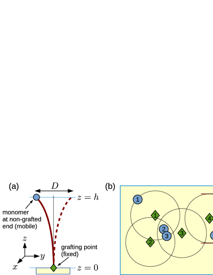
Figure 1: (a) Side-view of a single polymer chain, grafted perpendicularly onto a substrate. The grafted end (diamond) at $z=0$ is fixed; monomers at $z>0$ make thermal excursions about the average perpendicular orientation of the chain. We consider only the monomer at the non-grafted end (circle), whose motion is assumed to be confined to a circular region of diameter $D$ in the plane $z=h$. (b) Top-down view of a polymer brush containing $N=4$ chains. For each chain $i$, only the projected position $\vec{g}_{i}=(X_{i},Y_{i})$ of the grafting point is retained (diamonds), as well as the projected position $\vec{e}_{i}=(x_{i},y_{i})$ of the monomer at the non-grafted end (circles). The positions $\vec{e}_{i}$ are mobile, but their motion is restricted to a circular region of diameter $D$ around $\vec{g}_{i}$.

II Model

The essentials of our coarse grained model are summarized in Fig. 1. We consider polymer chains perpendicularly grafted on a substrate; an example of a single chain is shown in Fig. 1(a). We use Cartesian coordinates $(x,y,z)$, with $z$ the direction perpendicular to the substrate, and $x,y$ the lateral directions. The substrate is at $z=0$. The polymer is assumed to be stiff, i.e. its length is well below the persistence length. The perpendicular orientation imposed at the grafted end is thus maintained, on average, along the entire chain. The monomer at the grafted end (diamond) is fixed, at position $(X,Y,0)$, and hence does not move. Further along the chain, thermal energy allows the monomers to fluctuate about the average perpendicular orientation. The monomer at the free end (circle) has the largest fluctuation; the magnitude of the latter is denoted $D$. We now make the further assumption that the $z$-coordinate of the end monomer varies only very little during the fluctuation. That is, its motion is confined to the plane $z=h$. The coordinate of the end monomer may thus be written as $(x,y,h)$. The key simplification of our model is to consider the motion of the end monomer projected onto the $xy$-plane (i.e. a “top-down” view). That is: only the lateral coordinates of the grafting point $\vec{g}=(X,Y)$ and of the end monomer $\vec{e}=(x,y)$ are retained, making the model strictly two-dimensional. The grafting position $\vec{g}$ is set once at the start of the simulation, and remains fixed thereafter. The position of the end monomer $\vec{e}$ is then allowed to fluctuate, within a circular region of diameter $D$ around the grafting point: $|\vec{e}-\vec{g}|<D/2$.

In our model, the actual polymer brush (i.e. an assembly of many polymer chains) thus resembles the sketch of Fig. 1(b). A set of grafting points $\vec{g}_{i}$ (diamonds) is distributed onto the $xy$-plane following some recipe and fixed there $(i=1,\ldots,N)$. To each grafting point $i$, we assign a single coordinate $\vec{e}_{i}$, denoting the center of mass of the corresponding end monomer (circles). Each $\vec{e}_{i}$ is then allowed to fluctuate within a circle of diameter $D$ around $\vec{g}_{i}$. Pattern formation, i.e. clustering of the end monomers, is expected to occur when the circles around the grafting points overlap, and when the end monomers attract each other.

In what follows, we consider $L_{x}\times L_{y}$ surfaces with periodic boundaries. The model parameters are the (1) typical distance between the grafting points with respect to the circle diameter $D$, which we express in terms of the (dimensionless) quantity $\rho D^{2}$, with $\rho=N/(L_{x}L_{y})$ the grafting density, (2) nature of the interactions between the end monomers, and (3) details of how the grafting points are positioned (here: random versus non-random). In a real system, the diameter $D$ is set by the length of the polymer chains in relation to the persistence length and could, in principle, be calculated from the material properties.

III Method

We specialize to the case where the end monomers are point particles, and that closeby monomers attract (for readability, we drop the prefix “end” and simply speak of “monomers” from now on). The attraction is a short-ranged pair potential: Whenever two monomers $i$ and $j$ are within a distance $a$ of each other, $|\vec{e}_{j}-\vec{e}_{i}|<a$, the energy is lowered by an amount $\epsilon$. Our goal is to find low-energy configurations, and determine if these feature long-ranged order.

To further simplify matters, we consider the limit $a\to 0$, and use a Monte Carlo optimization scheme to find the low-energy configurations. The details of the scheme are as follows: First, the positions of the $N$ grafting points are generated. Next, a random location $\vec{r}_{1}$ is selected in the plane, and the grafting points for which $|\vec{g}-\vec{r}_{1}|<D/2$ are identified (assume there are $n$ such points). The corresponding monomers are then placed at $\vec{r}_{1}$, creating a monomer cluster of size $n$; the latter lowers the energy by an amount $\epsilon n(n-1)/2$. Note that $n=1$ is explicitly allowed; the starting configuration may thus be regarded as a system of $N$ isolated clusters. The process continues with a second random location $\vec{r}_{2}$, leading to the (proposed) creation of a second cluster (of size $n_{2}$), which we accept with the Metropolis probability $P=\min[1,e^{-\Delta E}]$. Here, $\Delta E$ is the energy difference between the initial and proposed configuration. If $|\vec{r}_{2}-\vec{r}_{1}|>D$, then $\Delta E=-\epsilon n_{2}(n_{2}-1)/2$. Otherwise, some of the monomers used to create the second cluster were “stolen” from the first, in which case there will be a second (positive) contribution to $\Delta E$. These steps are repeated many times, where each time $\Delta E$ must be carefully calculated (as the number of clusters increases, the creation of a new cluster generally involves the removal of monomers from other clusters). We also used a second Monte Carlo step, in which a grafting point was randomly selected, and the corresponding monomer “transferred” from its present cluster to a (randomly selected) other cluster in the vicinity, then accepted conform Metropolis; both types of move were attempted with equal a priori probability.

For $\epsilon>0$, one typically observes a rapid decrease of the energy with the number of steps. We emphasize that $\epsilon$ is merely a (dimensionless) parameter to set the convergence rate of the energy minimization. One should not regard $\epsilon$ as the analogue of inverse temperature. Indeed, the Monte Carlo moves are not ergodic, nor do they obey detailed balance, and so the scheme cannot be expected to sample the Boltzmann distribution at finite temperature. The sole purpose of our scheme is to find low-energy configurations: Given a set of grafting points $\vec{g}$, it finds energetically favorable positions for clusters of monomers, as well as the number of monomers each cluster contains. Note that the monomer positions $\vec{e}$ are not used. This presents an additional coarse graining step, which further aids to bridge the gap toward large length scales.

IV Results

Figure 2: Results for regularly placed grafting points at density $\rho D^{2}=64$. Left: Histogram $H(n)$ counting the observed cluster sizes $n$. The histogram is bimodal, allowing for a distinction between small and large clusters. Right: Snapshot showing the largest clusters (containing $n>25$ monomers). A hexagonal lattice, with lattice spacing $D$, is revealed.

We first consider $N=16560$ grafting points placed regularly on the sites of a square lattice, with lattice spacing $d/D=0.125$ (corresponding to grafting density $\rho D^{2}=64$). We start the energy minimization with $\epsilon=0$; every $10^{7}$ Monte Carlo steps, $\epsilon$ is increased by an amount 0.01 (with probability 70%) or decreased by the same amount (in the remaining cases). We thus allow for large structural changes initially (when $\epsilon$ is still small) which are gradually “frozen-out” as $\epsilon$ increases. For the present $N$, a typical minimization run requires $\sim 10^{10}$ steps, after which the energy does not decrease significantly anymore (this takes about 10 hours of CPU time).

In the left panel of Fig. 2, we show the histogram $H(n)$ of the observed cluster sizes $n$ obtained after one such run. The histogram is distinctly bimodal, i.e. there is a clear “cut-off”, at $n\sim 25$, separating small clusters from large ones. The right panel shows the positions of the large clusters, which have strikingly “crystallized” into a hexagonal lattice, with lattice spacing $D$. This result is to be expected: A large cluster can accommodate $\rho\pi(D/2)^{2}\sim 50$ monomers, corresponding to the right peak in the histogram. Under energy minimization, these clusters try to pack as densely as possible, explaining the hexagonal structure. However, not all monomers can participate in the hexagonal structure, as the packing fraction of the latter is only $\eta=\pi\sqrt{3}/6\sim 0.9$. The remaining monomers thus form smaller clusters, explaining the left peak in the histogram.

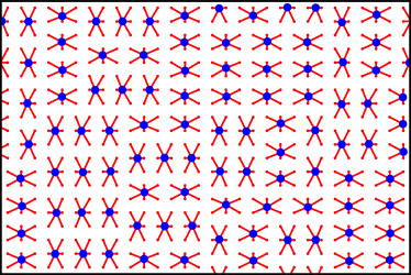
Figure 3: Snapshot corresponding to $N=600$ grafting points, placed on the sites of a square lattice, with lattice spacing $d/D=0.425$. The dots mark the positions of the monomer clusters; the lines show the connection of each grafting point to its corresponding cluster. Each cluster is a rectangular plaquette of $3\times 2$ monomers, which can be oriented horizontally or vertically; lamellar long-ranged order does not occur.

A prerequisite for the hexagonal structure is that the distance between the grafting points is small compared to $D$. Alternatively formulated, the grafting density $\rho D^{2}\gg 1$. If this condition is not met, then the low-energy configuration is largely determined by the lattice onto which the grafting points are placed (presently a square lattice). This we verify in Fig. 3, which shows a low-energy configuration where the spacing between the grafting points $d/D=0.425$ (corresponding to grafting density $\rho D^{2}\sim 5.5$, i.e. more than one order of magnitude lower compared to Fig. 2). We now observe a structure whereby each cluster occupies the center of a rectangular plaquette. The number of monomers per plaquette $n=(v+1)\times(w+1)$, $v={\rm int}(D/d)$, $w={\rm int}(\sqrt{(D/d)^{2}-v})$, where “int” means rounding-down to the nearest integer (for the present parameters, the plaquette size is $3\times 2$). As Fig. 3 shows, the plaquettes orient both horizontally and vertically. Hence, to fulfill the plaquette size constraint, it is not necessary for the plaquettes to arrange into regular lamellae. The resulting structure thus remains disordered. We emphasize that the structure of Fig. 3 likely is of little experimental relevance, as the number of polymer chains within a cluster is ${\cal O}(100)$ in experiments citeulike:6561954 .

Finally, we consider randomly placed grafting points. In this case, identifying the low-energy configurations is more difficult. For a given sample of (randomly placed) grafting points, there are typically many low-energy states. When $\epsilon$ becomes large, our minimization scheme “gets stuck” in one of these, but there is no guarantee that the resulting state is the groundstate (it likely is not). For this reason, it is necessary to perform several minimization runs for each sample of grafting points, and from these keep the configuration with the lowest energy. This still does not guarantee that the groundstate is found, but at least the probability of accidentally selecting a high-energy state is reduced. A single minimization run starts with $\epsilon=0$ to randomize the system; every $10^{6}$ Monte Carlo steps, $\epsilon$ is increased by 0.01, up to a maximum $\epsilon_{\rm max}=1.5$. For each sample of grafting points, we typically performed $\sim 50$ such runs.

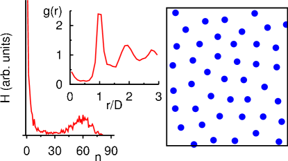
Figure 4: Results for randomly placed grafting points at density $\rho D^{2}=64$. Left: Histogram $H(n)$ of the observed cluster sizes $n$. The histogram is bimodal, but with overlapping peaks. Center: RDF $g(r)$ of the cluster-cluster pair correlations, reflecting the structure of a disordered fluid. Right: Typical snapshot of the largest ($n>25$) clusters, showing the absence of hexagonal order. Note: The histogram and RDF data were averaged over 25 samples of grafting points; the number of grafting points $N=2640$.

In Fig. 4 (left panel), we show the histogram of observed cluster sizes for grafting density $\rho D^{2}=64$, which is the same density of Fig. 2. We again observe a bimodal distribution, but with broader and overlapping peaks. One could still take the minimum between the peaks, at $n\sim 25$, as a “cut-off” separating small clusters from large ones. However, in contrast to regularly placed grafting points, the large clusters do not form a hexagonal lattice (right panel). Further confirmation that long-ranged order is absent follows from the radial distribution function $g(r)$ (RDF) of the cluster-cluster pair correlations (center panel). The RDF was calculated as follows: For all pairs of clusters $ij$, we computed the distance $r_{ij}$ between them; the latter were “binned” in a histogram $H(r)\propto rg(r)$, with each $r_{ij}$ counted $n_{i}n_{j}$ times ($n_{i}$ is the number of monomers in cluster $i$). We observe a RDF characteristic of a disordered fluid, i.e. there is some structure at short $r$, but for large $r$ the RDF tends to a constant. Note the pronounced peak at $r=D$, which reflects the typical distance between large clusters.

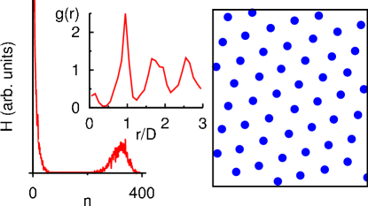
Figure 5: The analogue of Fig. 4, but using a larger grafting density $\rho D^{2}=400$. At this density, hexagonal order appears to be restored. The data correspond to $N=16560$ (randomly placed) grafting points; the snapshot shows the clusters containing $n>150$ monomers.

Next, we repeat the analysis using a larger grafting density $\rho D^{2}=400$, but still placing the grafting points randomly [Fig. 5]. At this density, the peaks in the cluster size histogram are again well separated, suggesting that hexagonal order is restored. Indeed, as the snapshot shows, the largest clusters have formed a hexagonal lattice. The peaks in the RDF have also become sharper, including clearly resolved second and third neighbor peaks.

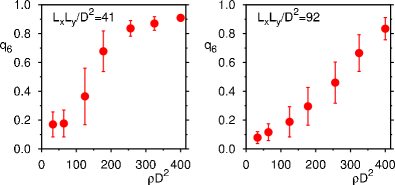
Figure 6: The hexatic order parameter $q_{6}$ of the low-energy configurations versus the grafting density $\rho$ for two values of the system area $L_{x}L_{y}$ as indicated (randomly placed grafting points). The error bars show the root-mean-square variation in the observed $q_{6}$ values between different samples of grafting points. The data indicate that, for $\rho$ large enough, hexatic order is restored.

Upon increasing the grafting density, the corresponding groundstate configurations thus appear to develop hexagonal order. To further quantify this, we measure the hexatic order parameter citeulike:12820541 of the groundstate configurations $q_{6}=|\sum_{[ij]}w_{ij}e^{\imath 6\theta_{ij}}|/\sum_{[ij]}w_{ij}$, $w_{ij}=n_{i}n_{j}$, with the sums over all cluster pairs $ij$ for which $0.5<r_{ij}/D<1.5$ (corresponding to the nearest-neighbor peak in the RDF). In the above, $\theta_{ij}$ is the angle of the vector connecting $i$ and $j$ with respect to an arbitrary reference. As in the RDF computation, we weigh each pair by the product of the number of monomers in each cluster. In Fig. 6, we plot $q_{6}$ versus the grafting density $\rho$, for two values of the system area $L_{x}L_{y}$. In both cases, $q_{6}$ increases with $\rho$, demonstrating that hexagonal order is restored at large grafting densities. There is, however, a strong system size dependence: In the larger system (right panel), the crossover to hexatic order occurs at larger $\rho$. These size effects could imply a geometric phase transition in the thermodynamic limit, at grafting density $\rho^{\star}$, below (above) which the groundstate configurations are disordered (hexagonally ordered). Consistent with a phase transition is the root-mean-square variation in the observed $q_{6}$ values between different samples of grafting points (indicated by the error bars). In the regime where $q_{6}$ rises most steeply, large variations are observed, suggesting a diverging susceptibility. Of course, to determine the precise scenario requires a finite-size scaling analysis, for which the data of Fig. 6 are unfortunately not accurate enough.

V Discussion

In summary, we have presented a highly coarse-grained model to describe lateral domain formation in polymer brushes. In this model, each polymer chain is specified by its grafting location on the substrate, and the position of the monomer at the non-grafted end. We then focus on the collective behavior of the latter monomers, whose positions are projected onto the grafting plane, resulting in a model that is strictly two-dimensional. Due to its simplicity, this model is able to probe pattern formation on the scale of polymer clusters, whereby each cluster may easily comprise several hundreds of polymer chains.

We considered this model in the case where the end monomers are point particles, without possessing any excluded volume of their own, and with an attractive pair potential between them. In the limit where the range of the attraction tends to zero, a further simplification becomes possible, whereby only the positions of the polymer clusters are retained. The latter are two-dimensional coordinates, a single one of which capturing the degree of freedom of many polymer chains. A Monte Carlo scheme was used to identify cluster coordinates that minimize the energy.

Our main finding is that, provided the grafting density is large enough, polymer clusters form hexagonal lattices under energy minimization. This finding holds irrespective of whether the polymer chains are grafted onto the substrate in a regular pattern, or placed randomly. In case of random grafting, the grafting density must exceed a significant threshold, $\rho^{\star}D^{2}\sim 300-400$, before hexagonal order is observed [Fig. 6]. These results make sense assuming that, under energy minimization, clusters aim to maximize their size (expressed in the number of monomers). For regularly placed grafting points, this maximum is a constant $n_{\rm max}\sim\rho\pi(D/2)^{2}$. The groundstate is the one which packs the clusters most efficiently, i.e. a hexagonal lattice [Fig. 2]. For random grafting, the number of grafting points inside a circle of diameter $D$ is a stochastic variable, $n_{\rm max}$ on average, but with Poisson fluctuations $\pm\sqrt{n_{\rm max}}$. This facilitates a second mechanism to minimize the energy, namely to form clusters where the grafting density locally is large (favoring disorder). At low grafting density, where the relative Poisson fluctuation $\sqrt{n_{\rm max}}/n_{\rm max}$ is largest, the latter mechanism dominates, yielding a disordered structure [Fig. 4]. As $\rho$ increases, the fluctuation vanishes; for $\rho>\rho^{\star}$, the first mechanism dominates again, leading to hexagonal order [Fig. 5].

It is interesting to compare our findings with the simulations of Ref. citeulike:6561954, . In the latter, it was concluded that randomly grafted polymers generally prevent the formation of ordered structures. Our conclusion is that order can arise, provided the grafting density exceeds $\rho^{\star}$ (implying that the grafting density of Ref. citeulike:6561954, is below $\rho^{\star}$). Since long-ranged order is also not observed in experiments citeulike:13045005 ; citeulike:12963613 , it may be that $\rho^{\star}$ is actually beyond reach in applications. For $\rho<\rho^{\star}$, large clusters are “pinned” to regions with a local excess in the grafting density citeulike:6561954 . As $\rho$ increases, and hexagonal order in the groundstate develops, we expect the pinning effect to vanish. For regularly placed grafting points, the simulations of Ref. citeulike:6561954, do observe a tendency toward order, consistent with our results. In this case, the requirement for order is that the distance between the grafting points is small compared to $D$, such that the influence of the grafting lattice is “washed out” (avoiding artifact structures of the type shown in Fig. 3).

Irrespective of the distribution of the grafting points, provided $\rho>\rho^{\star}$, we expect a phase transition between the disordered state at high temperature, and the ordered one at low temperature. This transition, presumably first-order, was not actually observed in Ref. citeulike:6561954, , nor ruled out. The theory of Ref. citeulike:12963558, predicts that the disordered state becomes unstable under appropriate conditions, implying that a phase transition must occur, but the nature of the transition could not be determined. Our present algorithm cannot answer this question either, since thermal fluctuations are ignored. However, the mere observation of an ordered groundstate makes it likely that a transition must occur. Of course, when $\rho<\rho^{\star}$, the brush remains disordered at all temperatures, precluding a phase transition.

For the future, two applications come to mind. The first is to replace our approximate Monte Carlo minimization scheme with an exact approach based on graph theory (this would facilitate a precise determination of $\rho^{\star}$). To this end, one regards the grafting points as vertices, with edges between vertices whose separation is less than $D$. One then determines the cliques of the resulting graph; the latter are sub-graphs whereby each vertex is connected to every other vertex. The largest cliques yield the optimal locations for polymer clusters (provided the diameter of the minimal enclosing circle around the clique does not exceed $D$). We have had some initial success with this approach; the remaining problem is how to distribute the clusters over the optimal locations.

The second application is to include thermal fluctuations. In case the range of attraction between monomer pairs $a>0$, a finite-temperature simulation is easily conceived: As Monte Carlo step, one randomly chooses a monomer, proposes a new random location for this monomer around its grafting point, and accepts conform Metropolis. Unfortunately, this scheme is inefficient for strong attractions: Once clusters have formed, they are extremely long-lived, and so equilibration is difficult (for this reason we focused on the groundstates for now). To capture thermal fluctuations, it seems more promising to remain in the limit $a\to 0$, and to modify the Monte Carlo minimization steps of this work such that ergodicity and detailed balance are obeyed. The details of these modifications are, however, not a priori obvious.

- (1) Ayres N, Polymer brushes: Applications in biomaterials and nanotechnology, Polym. Chem. 1, 769 (2010)
- (2) Price AD, Hur SM, Fredrickson GH, Frischknecht AL, and Huber DL, Exploring Lateral Microphase Separation in Mixed Polymer Brushes by Experiment and Self-Consistent Field Theory Simulations, Macromolecules 45, 510 (2011)
- (3) Norizoe Y, Jinnai H, and Takahara A, Molecular simulation of 2-dimensional microphase separation of single-component homopolymers grafted onto a planar substrate, EPL 16006 (2013)
- (4) Hur SM, Frischknecht AL, Huber DL, and Fredrickson GH, Self-assembly in a mixed polymer brush with inhomogeneous grafting density composition, Soft Matter 9, 5341 (2013)
- (5) Benetatos P, Terentjev EM, and Zippelius A, Bundling in brushes of directed and semiflexible polymers, Phys. Rev. E 88, 042601 (2013)
- (6) Wenning L, Müller M, and Binder K, How does the pattern of grafting points influence the structure of one-component and mixed polymer brushes?, EPL 71, 639 (2005)
- (7) Yeung C, Balazs AC, and Jasnow D, Lateral instabilities in a grafted layer in a poor solvent, Macromolecules 26, 1914 (1993)
- (8) Marko JF and Witten TA, Phase separation in a grafted polymer layer, Phys. Rev. Lett. 66, 1541 (1991)
- (9) Brown G, Chakrabarti A, and Marko JF, Microphase Separation of a Dense Two-Component Grafted-Polymer Layer, EPL 25, 239 (1994)
- (10) Zhao W, Krausch G, Rafailovich MH, and Sokolov J, Lateral Structure of a Grafted Polymer Layer in a Poor Solvent, Macromolecules 27, 2933 (1994)
- (11) Nelson D and Halperin B, Dislocation-mediated melting in two dimensions, Phys. Rev. B 19, 2457 (1979)