Prediction of the thermophysical properties of molten salt fast reactor fuel from first-principles

Abstract

Molten fluorides are known to show favorable thermophysical properties which make them good candidate coolants for nuclear fission reactors. Here we investigate the special case of mixtures of lithium fluoride and thorium fluoride, which act both as coolant and fuel in the molten salt fast reactor concept. By using ab initio parameterized polarizable force fields, we show that it is possible to calculate the whole set of properties (density, thermal expansion, heat capacity, viscosity and thermal conductivity) which are necessary for assessing the heat transfer performance of the melt over the whole range of compositions and temperatures. We then deduce from our calculations several figures of merit which are important in helping the optimization of the design of molten salt fast reactors.

I Introduction

The molten salt fast reactor (MSFR) is currently the most advanced concept of nuclear fission reactor involving the use of molten salts both as coolant and as fuel [1]. A great deal of research has recently been devoted to the optimization of its neutronic [2, 3], safety [4], recycling [5, 6, 7, 8, 9] and thermodynamic [10, 11, 12] characteristics. Its advantages are an intrinsic safety of the core, due to very negative feedback coefficients, a high working temperature which ensures a good efficiency, and the possibility to perform online refuelling and on-site treatment. But of particular interest is its high compositional flexibility. In particular, our precognized liquid fuel is a mixture of lithium fluoride and thorium fluoride (LiF-ThF₄). Being able to develop fission reactors based on the thorium cycle ensures a good availability of the resources for many countries. From the point of view of basic research, a consequence of the MSFR compositional flexibility is the need to generate substantial databases providing the variation of the properties of the melt with composition and temperature.

Due to the high temperature and to the corrosive character of molten fluorides, measuring their thermophysical properties is not a straightforward task, and the experimental results are generaly limited to pure salts or binary mixtures at the eutectic composition [13, 14, 15]. An efficient alternative is to use computer simulations. In particular, molecular dynamics (MD) simulations are able to provide all the necessary properties, such as the density, the heat capacity, the viscosity and the thermal conductivity. The necessary ingredients are a good model for the ionic interactions, and its associated parameters. In recent years, we have developed from first-principles, i.e. without involving any empirical information during the parameterization procedure, such interaction potentials for molten fluorides, in the framework of the polarizable ion model [16, 17, 18]. They were tested against many physical properties, as well as on diffraction and spectroscopy experiments. An excellent agreement was obtained for the full set of data [19, 20, 21]. In particular, for LiF-ThF₄ eutectic mixture, which corresponds to a ThF₄ mole fraction $x$ = 0.22, the largest deviation from experimental data observed was 5 % for the density [22]. Such a good predictive power from MD simulations has not been obtained yet for water, for example. It is thus possible to perform simulations under a large variety of thermodynamic conditions in order to feed the databases. In this work, we focus on the LiF-ThF₄ binary system, for which we calculate all the relevant physical properties over the whole range of compositions and temperatures. This allows us to map the variations of the thermophysical figures of merit which are necessary for the engineering of MSFRs.

II Model and methods

The pair additive form of the interionic potential includes charge-charge, charge-dipole, dipole-charge, dipole-dipole, repulsion, and two dispersion interaction terms, as follows :

$$U_{ij}\left({\bf r}_{ij}\right) = \frac{q_{i}q_{j}}{r_{ij}}+\frac{q_{i}{\bf r}_{ij}\cdot{\bm{\mu}}_{j}}{r_{ij}^{3}}f^{ij}_{4}\left(r_{ij}\right)-\frac{{\bm{\mu}}_{i}\cdot{\bf r}_{ij}q_{j}}{r_{ij}^{3}}f^{ji}_{4}\left(r_{ij}\right)$$ (1)

$$+\frac{{\bm{\mu}}_{i}\cdot{\bm{\mu}}_{j}}{r_{ij}^{3}}-\frac{3({\bf r}_{ij}\cdot{\bm{\mu}}_{i})({\bf r}_{ij}\cdot{\bm{\mu}}_{j})}{r_{ij}^{5}}$$

$$+B_{ij}\exp\left(-\alpha_{ij}r_{ij}\right)-\frac{C^{ij}_{6}}{r_{ij}^{6}}f^{ij}_{6}\left(r_{ij}\right)-\frac{C^{ij}_{8}}{r_{ij}^{8}}f^{ij}_{8}\left(r_{ij}\right)$$

where $q_{i}$ and ${\bm{\mu}}_{i}$ are the charge and dipole moment of particle $i$, respectively, and $f_{n}^{ij}$ the damping function for short-range correction of interactions between charge and dipole and dispersion interactions [23]:

$$f^{ij}_{n}(r^{ij})=1-c_{n}^{ij}{\rm e}^{-b_{n}^{ij}\times r^{ij}}\sum_{k=0}^{n}\frac{(b_{n}^{ij}\times r^{ij})^{k}}{k!}.$$ (2)

$\{B_{ij},\alpha_{ij},C^{ij}_{6},C^{ij}_{8},b_{n}^{ij},c_{n}^{ij}\}$ are a set of parameters which were determined from first-principles calculations in our previous works [22]. The dipole moment induced on each ion is a function of the polarizability and electric field on the ion caused by the charges and the dipole moments of all the other ions. The instantaneous dipole moment is determined self-consistently at every time step by minimization of the total energy using the conjugate gradient method. The charge-charge, charge-dipole, and dipole-dipole contributions to the potential energy and forces on each ion are evaluated under periodic boundary conditions by using the Ewald summation technique [24].

A first series of MD simulations was performed in the $NPT$ ensemble, where $N$ is the particle number included in the simulation cell, $P$ is the pressure which was always set to 1 atm and $T$ is the temperature. The barostat and thermostat relaxation times were both set to 10 ps. This allowed us to determine the equilibrium density at a given thermodynamic point. Then a second series of simulations was performed at fixed density, i.e. in the $NVT$ ensemble where $V$ is the volume. The same relaxation time was used for the thermostat. The simulation timestep was 0.5 fs, and the total simulation time was 0.25 ns and 7.5 ns for the $NPT$ and $NVT$ simulations, respectively. All the calculation conditions are summarized in the supplementary information; in total the system was simulated at 62 thermodynamic points with this procedure.

III Results and discussion

FOM	Convection	Régime	$r$	$s$	$t$	$u$	$v$	$w$
1	Forced	Turbulent	1.00	0.2	0.0	2.0	2.8	0.0
2	Natural	Turbulent	0.36	0.2	1.0	2.0	1.8	0.0
3	Natural	Laminar	0.50	1.0	1.0	2.0	1.0	0.0
4	–	–	1.00	0.2	1.0	0.3	0.6	0.6

Table 1: Coefficients for the figures of merit used to evaluate the heat-transfer properties of molten fluorides [25]. FOM4 is used for the heat-exchanger area.

Our ab initio-parameterized interaction potentials have been validated against many experimental data for similar systems. More precisely, they are able to reproduce with very high accuracy the measured EXAFS spectra [20] (LiF-ZrF₄, NaF-ZrF₄ and KF-ZrF₄), the Raman spectra [26] (LiF-BeF₂), the X-ray diffraction [27] (LiF-BeF₂), the electrical conductivity [21] (LiF-NaF-ZrF₄ and LiF-YF₃), the diffusion coefficients [28, 21] (LiF-KF and LiF-YF₃), the heat capacity [14] (CsF) and the viscosity [27] (LiF-BeF₂). For the thermal conductivity, this quantity is very difficult to measure experimentally and our simulations have shown an excellent agreement in the case of molten chlorides [29], for which accurate measurements could be made by using a method based on forced Rayleigh scattering. In the case of LiF-ThF₄, in our previous work [22] we have evaluated the density, the viscosity and the electrical conductivity at the eutectic composition. Our MD results showed a very good agreement with the corresponding experimental data [13]. In the present work, we can therefore consider our simulations to provide us accurate predictions.

In order to compare the performances of a series of coolants, it is useful to define generalized heat-transfer metrics. Several figure of merits (FOM) have been proposed by Bonilla to evaluate the properties of molten fluorides as coolants for nuclear reactors [25]. They take the following general form:

$${\rm FOM}=\left(\frac{\eta^{s}}{\beta^{t}\rho^{u}C_{p,m}^{v}\lambda^{w}}\right)^{r}$$ (3)

where $\eta$ is the viscosity, $\beta$ the thermal expansion, $\rho$ the density, $C_{p,m}$ the massic heat capacity at fixed pressure and $\lambda$ the thermal conductivity of a given melt. The set of exponents $r$, $s$, $t$, $u$, $v$ and $w$ vary depending on the conditions. The corresponding values are summarized in Table 1.

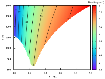
Figure 1: Variation of the density of the LiF-ThF₄ melts with composition and temperature. The white region corresponds to temperatures below the liquidus.

Our objective is to map the variations of all the properties which are necessary for determining the FOMs over the whole range of temperatures and compositions. We have therefore tried to fit all the simulation data with simple analytic functions, by finding the parameters which allow to minimize

$$\chi^{2}(a)=\frac{1}{N_{\rm sim}}\sum_{i=1}^{N_{\rm sim}}\left(\frac{a_{i}(x,T)-a_{i}^{\rm MD}}{a_{i}^{\rm MD}}\right)^{2}$$ (4)

where $a_{i}^{\rm MD}$ is the value extracted from the MD simulation for the property $a$ at a given thermodynamic point ($N_{\rm sim}$ is the total number of simulated points) and $a_{i}(x,T)$ is the corresponding value for the analytical function ($x$ is the mole fraction of ThF₄ in the melt and $T$ the temperature), which contains the parameters which need to be fitted.

First we start with the density. For this quantity, a small temperature dependence has to be included since this quantity usually varies linearly with temperature at fixed composition [13, 22]. An excellent fit of the simulation data was obtained by using the following polynomial expression:

$$\rho(x,T) = 2.2247-0.0004329\times T$$ (5)

$$+(15.412-0.0015748\times T)\times x$$

$$+(-8.1106-0.0088374\times T)\times x^{2}$$

$$+(-11.380+0.020484\times T)\times x^{3}$$

$$+(9.2358-0.010673\times T)\times x^{4}$$

The average error is $\chi(\rho)$ = 1.5 %. The $\rho(x,T)$ map is plotted on Figure 1; unsuprisingly the largest variations are due to the composition changes, and larger densities are obtained for high ThF₄ concentrations due to the large difference of molar weight between the two cations.

The thermal expansion, which corresponds to the material’s volume change as a function of temperature, was derived from the simulation results using the following equation:

$$\beta=-\frac{1}{\rho}\left(\frac{\partial\rho}{\partial T}\right)_{P}$$ (6)

Its variation with temperature at fixed composition is negligible, and the following polynomial relation was fitted for the composition changes:

$$\beta(x,T)=\beta(x)=0.0001\times(3.0829-1.3187\times x-0.43862\times x^{2})$$ (7)

yielding a value of 0.8 % for $\chi(\beta)$.

Similarly, the heat capacity of molten salts is usually constant with respect to temperature variations at fixed composition. This is not the case for the corresponding solid phases [14]. Our simulations, in which the molar heat capacity $C_{p}$ is calculated by differentiation of the molar enthalpy $H$ (extracted from the $NPT$ ensemble simulations) with respect to the temperature,

$$C_{p}=\left(\frac{\partial H}{\partial T}\right)_{P},$$ (8)

confirm this behavior. Unlike other molten fluoride mixtures [30], for which a deviation from ideality was measured, in the LiF-ThF₄ melts $C_{p}$ varies almost linearly with composition. However, a fourth degree polynomial analytic function was fitted,

$$C_{p}(x,T) = C_{p}(x)=63.752+120.85\times x-115.22\times x^{2}$$ (9)

$$+171.86\times x^{3}-68.994\times x^{4}$$

yielding 0.1 % for $\chi(C_{p})$. In order to deduce the massic heat capacity, we need to divide $C_{p}$ by the molar weight $M$, which is given exactly by the relation

$$M(x)=(232.04+18.998\times 4.0)\times x+(6.94+18.998)\times(1-x)$$ (10)

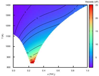
Figure 2: Variation of the viscosity of the LiF-ThF₄ melts with composition and temperature. The white region corresponds to temperatures below the liquidus.

The viscosity $\eta$ was determined by the Green-Kubo method, i.e. by integrating the correlation function of the stress tensor, as follows :

$$\eta=\frac{V}{k_{B}T}\int_{0}^{\infty}\langle\sigma_{\alpha\beta}(0)\sigma_{\alpha\beta}(t)\rangle{\rm d}t$$ (11)

in which $\sigma_{\alpha\beta}$ is one of the components of the stress tensor [31]. In order to improve the statistics, the stress autocorrelation function is averaged over the five independent components ($\sigma_{xy}$, $\sigma_{xz}$, $\sigma_{yz}$, $\sigma_{xx-yy}$ and $\sigma_{2zz-xx-yy}$). Much longer simulation times are needed to compute the viscosity, because enough statistics needs to be accumulated in order to yield a plateau for the integral defined in Equation 11.

In molten salts, the viscosity typically follows an Arrhenius law for the variation with temperature. We have therefore used a more complex analytic form than for the other properties,

$$\eta(x,T) = 0.21412\times\exp{\frac{2383.3}{T}}$$ (12)

$$+(0.022784\times\exp{\frac{7000.1}{T}})\times x$$

$$+(94.189\times\exp{\frac{-4807.0}{T}})\times x^{2}$$

$$+(-3.0284\times\exp{\frac{2281.7}{T}})\times x^{3}$$

$$+(0.76363\times\exp{\frac{4016.4}{T}})\times x^{4}$$

Although a larger overall error is observed, $\chi(\eta)$=9 %, it remains within the error bars of the MD simulation values. The variation of $\eta$ with respect to $x$ and $T$ is shown on Figure 2. Unlike other properties, the composition variation appears to be small. This behavior is different from other melts such as LiF-BeF₂ mixtures, for which viscosities larger by several orders of magnitudes are obtained on the BeF₂-rich side [32]. This is due to the strong network-forming ability of BeF₂, which is not observed for ThF₄. The largest viscosities are thus obtained for the lower temperatures, around the eutectic composition.

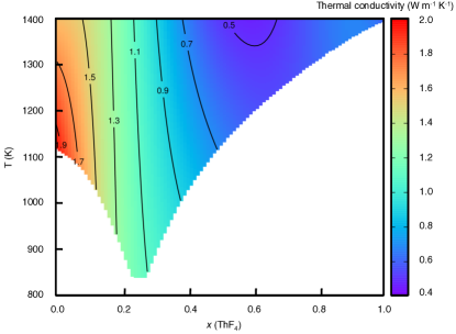
Figure 3: Variation of the thermal conductivity of the LiF-ThF₄ melts with composition and temperature. The white region corresponds to temperatures below the liquidus.

Finally, the thermal conductivity is the most complex quantity to calculate. Like the viscosity, it is obtained using the Green-Kubo method [29], but in that case several phenomelogical coefficients need to be calculated from the integration of the corresponding microscopic fluxes auto-correlation functions. Nevertheless, it was shown by Ohtori et al. that its temperature variation is very small, and is a consequence of the change of the density of the melt only [33]. We used the same analytic function as for the density, and the following expression was obtained.

$$\lambda(x,T) = 3.6014-0.0014497\times T$$ (13)

$$+(-24.140+0.017325\times T)\times x$$

$$+(87.337-0.072664\times T)\times x^{2}$$

$$+(-126.47+0.10924\times T)\times x^{3}$$

$$+(61.298-0.053182\times T)\times x^{4},$$

with $\chi(\lambda)$ = 5.9 %, which is again well within the simulation error bars. The $\lambda(x,T)$ map is plotted on Figure 3, interestingly we observe a minimum for a composition of $x$ = 0.6. Unlike the viscosity, the thermal conductivity of liquids does not show substantial variations when the structure of the melt changes (upon formation of a network, for example). Some efforts are currently made in order to improve our understanding of this quantity from the physical chemistry point of view in molten salts [33] as well as in molecular solvents such as water [34, 35].

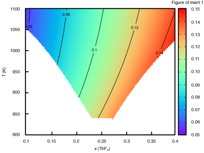
Figure 4: Variation of the FOM1 (forced convection, turbulent régime) of the LiF-ThF₄ melts with composition and temperature in the eutectic region. The white region corresponds to temperatures below the liquidus.

It is then possible to calculate the FOMs as defined by Equation 3 and the sets of exponents given in Table 1 at any thermodynamic point. The example of FOM1 in the eutectic region is shown on Figure 4; similar plots are provided for FOM2, 3 and 4 in the supplementary information. The smaller the FOM is, the better heat-transfer performance. We note that the FOMs of LiF-ThF₄ are relatively similar to those of LiF-NaF-KF and NaF-ZrF₄ eutectic mixtures [36], which are among the candidates for being used in another molten salt-based reactor, the advanced high temperature reactor [37]. The figure reveals that a LiF-rich melt is favorable for the thermal properties. Since the thorium is the fertile material, from which the fissile ²³³U is formed during the reactor operation, a compromise would have to be found for choosing an optimal composition for the reactor performance. Furthermore, one of the most important technological difficulties which needs to be overcome is to have container materials with a very high resistance to corrosion. A consequence of this is that the temperature has to be kept as low as possible, leading to composition choices close to the eutectic. The spatial variation of the temperature may be relatively large inside the reactor core. Here we observe that the FOMs tend to decrease with increasing temperature, which should ensure a good extraction of the heat at all the conditions.

IV Conclusion

The development of reliable interaction potentials, with ab initio accuracy, and the availability of large computer resources now allow us to build reliable thermophysical databases for molten salts. Such an approach is complementary to experimental measurements, yielding a large number of data at a very reasonable cost. In the present work we have illustrated this by calculating the density, the thermal expansion, the heat capacity, the viscosity and the thermal conductivity of LiF-ThF₄ mixtures for a wide range of compositions and temperatures. By fitting the calculated data with analytic functions, we have been able to map the variations of these properties for any thermodynamic point, and to determine the figures of merit which are necessary for designing molten salts reactor.

Although LiF and ThF₄ are the main components of the MSFR, it is sure that small amounts of other fluorides (UF₃, UF₄ and PuF₃, mainly) will also be present. In addition a large number of species will be formed due to the fission and the neutron capture reactions, and it remains impossible to extend the present work for all the elements. Therefore only the most important ones can be considered. However this difficulty can be overcomed by using thermodynamic models, which have up to now been fitted on experimental data only. The improvement of the thermodynamic models by the inclusion of the large amount of data provided by MD simulations should allow for the extension of the range of their applicability in the future.

References

- [1] G. Locatelli, M. Mancini, and N. Todeschini. Generation IV nuclear reactors: Current status and future prospects. Energ. Policy, 61:1503–1520, 2013.
- [2] L. Mathieu, D. Heuer, R. Brissot, C. Garzenne, C. Le Brun, D. Lecarpentier, E. Liatard, J. M. Loiseaux, O. Meplan, E. Merle-Lucotte, A. Nuttin, E. Walle, and J. Wilson. The thorium molten salt reactor: moving on from the MSBR. Prog. Nucl. Energy, 48:664–679, 2006.
- [3] M. Aufiero, M. Brovchenko, A. Cammi, I. Clifford, O. Geoffroy, D. Heuer, A. Laureau, M. Losa, L. Luzzi, E. Merle-Lucotte, M. E. Ricotti, and H. Rouch. Calculating the effective delayed neutron fraction in the molten salt fast reactor: Analytical, deterministic and monte carlo approaches. Ann. Nucl. Energy, 65:78–90, 2014.
- [4] M. Brovchenko, D. Heuer, E. Merle-Lucotte, M. Allibert, V. Ghetta, A. Landreau, and P. Rubiolo. Design-related studies for the preliminary safety assessment of the molten salt fast reactor. Nucl. Sci. Eng., 175:329–339, 2013.
- [5] S. Delpech, E. Merle-Lucotte, D. Heuer, M. Allibert, V. Ghetta, C. Le-Brun, X. Doligez, and G. Picard. Reactor physics and reprocessing scheme for innovative molten salt reactor system. J. Fluorine Chem., 130:11–17, 2009.
- [6] C. Hamel, P. Chamelot, A. Laplace, E. Walle, O. Dugne, and P. Taxil. Reduction process of uranium (IV) and uranium (III) in molten fluorides. Electrochim. Acta, 52:3995–4003, 2007.
- [7] M. Gibilaro, L. Massot, P. Chamelot, L. Cassayre, and P. Taxil. Electrochemical extraction of europium from molten fluoride media. Electrochim. Acta, 55:281–287, 2009.
- [8] P. Taxil, L. Massot, C. Nourry, M. Gibilaro, P. Chamelot, and L. Cassayre. Lanthanides extraction processes in molten fluoride media: Application to nuclear spent fuel reprocessing. J. Fluorine Chem., 130:94–101, 2009.
- [9] M. Gibilaro, L. Cassayre, O. Lemoine, L. Massot, O. Dugne, R. Malmbeck, and P. Chamelot. Direct electrochemical reduction of solid uranium oxide in molten fluoride salts. J. Nucl. Mater., 414:169–173, 2011.
- [10] O. Benes and R. J. M. Konings. Thermodynamic properties and phase diagrams of fluoride salts for nuclear applications. J. Fluorine Chem., 130:22–29, 2009.
- [11] O. Benes and R. J. M. Konings. Thermodynamic assessment of the LiF–CeF3–ThF4 system: Prediction of PuF3 concentration in a molten salt reactor fuel. J. Nucl. Mater., 435:164–171, 2013.
- [12] E. Capelli, O. Benes, M. Beilmann, and R.J.M. Konings. Thermodynamic investigation of the LiF-ThF4 system. J. Chem. Thermodyn., 58:110–116, 2013.
- [13] O. Benes and R.J.M. Konings. Molten salt reactor fuel and coolant. Comprehensive Nuclear Materials, 3:359–389, 2012.
- [14] O. Benes, R. J. M. Konings, D. Sedmidubský, M. Beilmann, O. S. Valu, E. Capelli, M. Salanne, and S. Nichenko. A comprehensive study of the heat capacity of CsF from T = 5 K to T = 1400 K. J. Chem. Thermodyn., 57:92–100, 2012.
- [15] V. Kohklov, I. Korzun, V. Dokutovich, and E. Filatov. Heat capacity and thermalconductivity of molten ternary lithium, sodium, potassium, and zirconium fluorides mixtures. J. Nucl. Mater., 410:32–38, 2011.
- [16] P. A. Madden, R. J. Heaton, A. Aguado, and S. Jahn. From first-principles to material properties. J. Mol. Struct.: THEOCHEM, 771:9–18, 2006.
- [17] M. Salanne and P. A. Madden. Polarization effects in ionic solids and melts. Mol. Phys., 109:2299–2315, 2011.
- [18] M. Salanne, B. Rotenberg, C. Simon, S. Jahn, R. Vuilleumier, and P. A. Madden. Including many-body effects in models for ionic liquids. Theor. Chem. Acc., 131:1143, 2012.
- [19] R. J. Heaton, R. Brookes, P. A. Madden, M. Salanne, C. Simon, and P. Turq A first-principles description of liquid BeF2 and its mixtures with LiF: 1. Potential development and pure BeF2. J. Phys. Chem. B, 110:11454–11460, 2006.
- [20] O. Pauvert, D. Zanghi, M. Salanne, C. Simon, A. Rakhmatullin, H. Matsuura, Y. Okamoto, F. Vivet, and C. Bessada. In situ experimental evidence for a nonmonotonous structural evolution with composition in the molten LiF-ZrF4 system. J. Phys. Chem. B, 114:6472, 2010.
- [21] M. Levesque, V. Sarou-Kanian, M. Salanne, M. Gobet, H. Groult, C. Bessada, and A.-L. Rollet. Structure and dynamics in yttrium-based molten rare earth alkali fluorides. J. Chem. Phys., 138:184503, 2013.
- [22] L. C. Dewan, C. Simon, P. A. Madden, L. W. Hobbs, and M. Salanne. Molecular dynamics simulation of the thermodynamic and transport properties of the molten salt fast reactor fuel LiF–ThF4. J. Nucl. Mater., 434:322–327, 2013.
- [23] K. T. Tang and J. P. Toennies. An improved simple model for the van der Waals potential based on universal damping functions for the dispersion coefficients. J. Chem. Phys., 80:3726–3741, 1984.
- [24] A. Aguado and P. A. Madden. Ewald summation of electrostatic multipole interactions up to the quadrupolar level. J. Chem. Phys., 119:7471–7483, 2003.
- [25] C. F. Bonilla. Nuclear Engineering Handbook, chapter 6.5, pages 9–90. 1958.
- [26] R. J. Heaton and P. A. Madden. Fluctuating ionic polarizabilities in the condensed phase: first-principles calculations of the Raman spectra of ionic melts. Mol. Phys., 106:1703–1719, 2008.
- [27] M. Salanne, C. Simon, P. Turq, R. J. Heaton, and P. A. Madden. A first-principles description of liquid BeF2 and its mixtures with LiF: 2. network formation in LiF-BeF2. J. Phys. Chem. B, 110:11461–11467, 2006.
- [28] V. Sarou-Kanian, A.-L. Rollet, M. Salanne, C. Simon, C. Bessada, and P. A. Madden. Diffusion coefficients and local structure in basic molten fluorides: in situ NMR measurements and molecular dynamics simulations. Phys. Chem. Chem. Phys., 11:11501–11506, 2009.
- [29] N. Ohtori, M. Salanne, and P. A. Madden. Calculations of the thermal conductivities of ionic materials by simulation with polarizable interaction potentials. J. Chem. Phys., 130:104507, 2009.
- [30] M. Beilmann, O. Benes, E. Capelli, V. Reuscher, R. J. M. Konings, and Th. Fanghänel. Excess heat capacity in liquid binary alkali-fluoride mixtures. Inorg. Chem., 52:2404–2411, 2013.
- [31] J.-P. Hansen and I.R. McDonald. Theory of simple liquids. Academic Press, 4th edition, 1986.
- [32] M. Salanne, C. Simon, P. Turq, and P. A. Madden. Simulation of the liquid-vapor interface of molten LiBeF3. C. R. Chim., 10:1131–1136, 2007.
- [33] N. Ohtori, T. Oono, and K. Takase. Thermal conductivity of molten alkali halides: temperature and density dependence. J. Chem. Phys., 130:044505, 2009.
- [34] F. Roemer and F. Bresme. Heat conduction and thermomolecular orientation in diatomic fluids: a non-equilibrium molecular dynamics study. Mol. Simulat., 38:1198–1208, 2012.
- [35] F. Roemer, A. Lervik, and F. Bresme. Nonequilibrium molecular dynamics simulations of the thermal conductivity of water: A systematic investigation of the spc/e and tip4p/2005 models. J. Chem. Phys., 137:074503, 2012.
- [36] M. Salanne, C. Simon, P. Turq, and P. A. Madden. Heat-transport properties of molten fluorides: determination from first-principles. J. Fluorine Chem., 130:38–44, 2009.
- [37] C. Forsberg. The advanced high-temperature reactor: high-temperature fuel, liquid salt coolant, liquid-metal-reactor plant. Progress in Nuclear Energy, 47:32–43, 2005.