Empirical symptoms of catastrophic bifurcation transitions
on financial markets: A phenomenological approach

M. Kozłowska marz.kozlowska@poczta.onet.pl Institute of Experimental Physics, Faculty of Physics
University of Warsaw, Hoża 69, PL-00681 Warsaw, Poland T. Gubiec Tomasz.Gubiec@fuw.edu.pl Institute of Experimental Physics, Faculty of Physics
University of Warsaw, Hoża 69, PL-00681 Warsaw, Poland T. R. Werner Tomasz.Werner@fuw.edu.pl Institute of Theoretical Physics, Faculty of Physics
University of Warsaw, Hoża 69, PL-00681 Warsaw, Poland M. Denys Mateusz.Denys@fuw.edu.pl Institute of Experimental Physics, Faculty of Physics
University of Warsaw, Hoża 69, PL-00681 Warsaw, Poland A. Sienkiewicz asien@okwj.edu.pl Institute of Experimental Physics, Faculty of Physics
University of Warsaw, Hoża 69, PL-00681 Warsaw, Poland R. Kutner Ryszard.Kutner@fuw.edu.pl (for_the_correspondence) Institute of Experimental Physics, Faculty of Physics
University of Warsaw, Hoża 69, PL-00681 Warsaw, Poland Z. Struzik zbigniew.struzik@gmail.com The University of Tokyo, 7-3-1 Hongo,
Bunkyo-ku, Tokyo 113-0033, Japan
and
RIKEN Brain Science Institute,
2-1 Hirosawa, Wako-shi 351-0198, Japan

Abstract

The principal aim of this work is the evidence on empirical way that catastrophic bifurcation breakdowns or transitions, proceeded by flickering phenomenon, are present on notoriously significant and unpredictable financial markets. Overall, in this work we developed various metrics associated with catastrophic bifurcation transitions, in particular, the catastrophic slowing down (analogous to the critical slowing down). All these things were considered on a well-defined example of financial markets of small and middle to large capitalization. The catastrophic bifurcation transition seems to be connected with the question of whether the early-warning signals are present in financial markets. This question continues to fascinate both the research community and the general public. Interestingly, such early-warning signals have recently been identified and explained to be a consequence of a catastrophic bifurcation transition phenomenon observed in multiple physical systems, e.g. in ecosystems, climate dynamics and in medicine (epileptic seizure and asthma attack). In the present work we provide an analogical, positive identification of such phenomenon by examining its several different indicators in the context of a well-defined daily bubble; this bubble was induced by the recent worldwide financial crisis on typical financial markets of small and middle to large capitalization.

pacs:

89.65.Gh, 02.50.Ey, 02.50.Ga, 05.40.Fb, 02.30.Mv

I Introduction

Discontinuous phase transitions in complex systems (much as in liquid-gas systems) together with critical phenomena are topics of canonical importance in statistical thermodynamics DS0 ; SCN ; LB ; BaPo ; DGM ; HH ; LWCBT . During the evolution of the complex systems we observed various catastrophic breakdowns proceeded by flickering phenomenon. This type of evolution is an example of a generic problem how small changes can lead to dramatic consequences. Overall, in this work we developed various metrics associated with catastrophic bifurcation transitions. All these things were considered on a well-defined example of notoriously significant and unpredictable financial markets MS ; BMR ; DiSo ; AJK ; MaSo ; JJH ; JF (and refs. therein).

The significant contribution to explanation of mechanism of financial market evolution, in particular the settlement of whether the early-warning signals are visible there, is a generic challenge of our work. Notably, the problem of whether the early-warning signals in the form of a critical slowing down phenomena (observed in multiple physical systems LB ; SCN ; LWCBT ) are present on financial markets was clearly formulated in ref. SBBB . Nowadays, as well critical as catastrophic slowing downs (the latter systematically considered in this work) seem to be the most refined indicators of whether a system is approaching a critical threshold or a bifurcation catastrophic tipping point, respectively GJ ; MQBR ; CB ; CBCKP ; BCS .

Our contribution can open possibilities for numerous applications, for instance, to forecasting, market risk analysis and financial market management. Econophysics – the physics of financial markets — offers particularly promising approaches to our challenge and therefore it constitutes a principal framework of our work Wiki .

The basic term of our work, i.e., the term ’complex system’ defines a system composed of a large number of interconnected entities – degrees of freedom, often open to its environment, self-organizing its internal structure and dynamics, expressing novel macroscopic or emergent properties. The paramount property of complex system is its indivisibility. For this reason, reductionist approaches fail in the case of complex systems which must be considered holistically.

Complex systems play an increasing role in majority of scientific disciplines. Notable examples can be drawn from biology and biophysics (biological networks, ecology, evolution, origin of life, immunology, neurobiology, molecular biology, etc), geology and geophysics (plate-tectonics, earthquakes and volcanoes, erosion and landscapes, climate and weather changes, environment evolution, etc.). Besides their essential role in the characterization of a range of phenomena in physics and chemistry, complex systems are now indispensable in economy (covering econometrics and financial markets) as well as in social sciences (including cognition, opinion dynamics, distributed learning, interacting agents, etc.).

The cross-disciplinary approach enabled the discovering of several features and stylized facts of financial market’s complexity. For instance, the approach stimulating our present work comes in part from ecology SBBB ; GJ ; DSDS , where sometimes ecosystem undergoes a catastrophic regime shift (in the sense of Réne Thom catastrophe theory GJ ), over relatively short period of time. This regime shift seems to be one of the most sophisticated because of bifurcation existence. This means that the catastrophe or tipping points DSDS ; AJ exist, at which a sudden shift of the system to a contrasting regime may occur¹¹1For instance, the sudden shifts (or jump discontinuities) of magnetization plotted versus magnetic field was already found, at critical fields, in our early physical work KBK , where we studied the influence of lattice ordering on diffusion properties.. Furthermore, before reaching a tipping point, there is also a possibility of the system transition to such a state, where system again continues its evolution gradually. This is a subcatastrophic bifurcation transition. Anyway, both kind of transitions, i.e., the catastrophic and subcatastrophic ones, are discontinuous that is, they are the analog of the first-order phase transitions DS0 .

One of the most important attainment of the catastrophe theory in the context of economics seems to be an introducing the complexity into it. For instance, already elementary catastrophes introduced a nonlinear topological complexity which was utilized within the different economical sectors ECZ -JBR .

There is a well-known controversy, concerning two-state transitions on financial markets, which is the significant inspiration of our work. Namely, Plerou, Gopikrishnan and Stanley PGS1 ; PGS2 observed a two-phase behavior on financial markets by using empirical transactions and quotes within the intra-day data for 116 most actively traded US stocks, for the two-year period 1994-1995. By examining the fluctuation of volume imbalance that is, by using some conditional probability distribution of the volume imbalance, they found the change of this distribution from uni- to bimodal one. That is, the market shifted from equilibrium to out-of-equilibrium state, where these two different states were interpreted as distinct phases.

In contradiction, Potters and Bouchaud PB pointed out that two-phase behavior of the above mentioned conditional distribution is a direct consequence of generic statistical properties of traded volume and not real two-phase phenomena.

Nevertheless, two-phase phenomenon was again examined for financial index DAX by Zheng, Qiu and Ren by using minority games and dynamic herding models ZQR . They found that this phenomenon is a significant characteristics of financial dynamics, independent of volatility clustering.

Moreover, Jiang, Cai, Shou and Zhou observed the bifurcation phenomenon for Hang-Seng index JCZZ as non-universal one, which requires specific conditions.

However, Matia and Yamasaki in his work MY on trading volume indicated that bifurcation phenomenon is an artifact of the distribution of trade sizes which follows a power-law distribution with exponent belonging to the Lévy stable domain.

Very recently, Filimonov and Sornette FS proved that the trend switching phenomena in financial markets considered by Preis et al. TP ; PSS ; PS ; PTS ; SBFHMKPP ; PTSE ; PTSHE has a spurious character. They argued that this character stems from the selection of price peaks that imposes a condition on the studied statistics of price change and of trade volumes that skew their distributions.

In the present work we consider the bifurcation phenomenon from complementary point of view because, we focus our attention on its unconditional catastrophic properties. The main goal of our complementary work is to provide some empirical facts for possible existing of catastrophic bifurcation transitions (CBT) of stock markets of small and middle to large capitalization. If several effects found in this work would be considered separately one could suppose that they have different sources. However, the fact that they appeared together indicates that their origin is in the catastrophic bifurcation transition.

The classification of crises as bifurcation between a stable regime and a novel regime provides a first step towards identifying signatures that could be used for prediction DS0 (and refs. therein). For instance, the problem of the tipping points existence in financial markets is a heavily researched area. This is because the discovery of predictability leads to its elimination according to the one of the fundamental financial market paradigm. This paradigm states that as profit can be made (for instance, from predictability), a financial market gradually annihilates such an arbitrage opportunity.

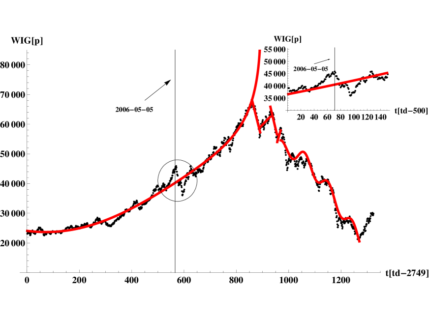
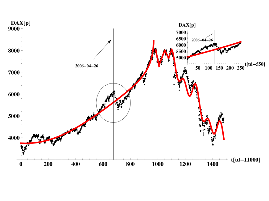
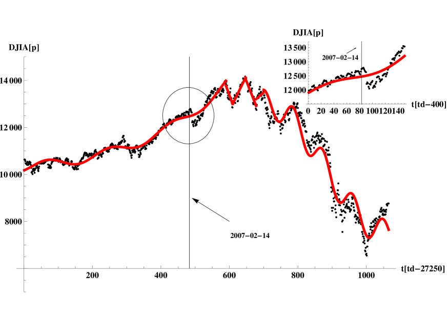
In this article we identify catastrophic bifurcation by verifying a list of its basic indicators, herein for WIG²²2The index WIG (Warszawski Indeks Giełdowy) is the main one of the Warsaw Stock Exchange, which is of a small size., DAX, and DJIA daily speculative bubbles on the Warsaw Stock Exchange, Frankfurter Wertpapierbörse, and New York Stock Exchange, respectively. That is, we mainly consider stock market speculative bubbles of recent worldwide financial crisis of small and middle to large capitalization (cf. Figures 1-3).

Refer to caption — Figure 1: The latest well formed peak of WIG (the erratic curve) beginning at 2004-02-06 (the $2480^{th}$ trading day (td) of the Warsaw Stock Exchange) and ended at 2009-05-18 (the $4075^{th}$ td). The maximum of empirical data is located at 2007-07-06 (the $3340^{th}$ td) while the corresponding theoretical maximum at 2007-08-22 (the $3372^{nd}$ td). The solid curve is our theoretical long-term (multi-year) trend KK fitted to the hossa (left-hand side of the peak). The dashed vertical line denotes the position of the local peak’s maximum placed at 2006-05-05. This is the most pronounced local peak defined relatively to the trend, which was presented separately (in the upper right corner of the figure) by the smaller plot.

In this work we pay our attention to the analysis of daily financial market data by considering them from the interdisciplinary point of view. We suppose that daily data is the most significant as they contain some reminiscences both from the high- as well as from the low-frequency trading. That is, the data have an intermediate character containing some informations both on the intra-day trading as well as on the less frequent longer-term inter-day one. Moreover, the detrending procedure of the daily data is better established than for the intra-day data because for the latter well known intra-day patterns exist. Both bullish and bearish sides of considered peaks are detrended herein by using generalized exponential (or Mittag-Leffler function) decorated by some oscillations (for details see Appendix A) because such a function slightly better fits peaks considered in this work than commonly used log-periodic function.

The content of the paper is as follows. In Section II we consider the structural transformation between graphs (trees), which constitutes environment for bifurcation transitions. The trees were calculated by MST technique and found as quite different before and during the recent worldwide financial crisis. Section III is devoted systematic empirical analysis of daily data originating from three typical stock markets of small, intermediate and large capitalization. In Section IV we explain how linear and nonlinear indicators arise when system approaches the catastrophic bifurcation threshold. Section V contains concluding remarks.

II Structural phase transitions on financial markets

Barely since about two decades, physicists have intensively studied the structural (or topological) properties of complex networks DGM (and refs. therein). They discovered that in the most real graphs small and finite loops are rare and insignificant. Hence, it was possible to assume their architectures as locally treelike; the property which has been extensively exploited. It is also surprise how well this simplification works in the case of numerous loopy and clustered networks. Therefore, we decided for the Minimal Spanning Tree (MST) technique as particularly useful, canonical tool of a graph theory BeBo being a correlation based network without any loop RNM ; BCLMVM ; MS ; BLM ; VBT ; KKK ; TMAM ; TCLMM (and refs. therein).

We consider a simple dynamics of the empirical network. That is, the network consists of the fix number of vertices where only distances between them can vary in time. Obviously, during the network evolution some of its edges can disappear while others can be born. Hence, the number of edges is a non–conserved quantity continuously varying in time likewise, for instance, their mean length and a mean occupation layer RNM ; BLM ; BR ; TSC .

We applied the MST technique to find the transition of complex network during its evolution from the hierarchical tree representing the stock market structure before the recent worldwide financial crash DiSo , to star like tree representing the market structure already comprising the crash. Subsequently, we found the transition from the latter tree to the hierarchical one decorated by several local star like trees (hubs) representing the market structure after the worldwide financial crash. These two types of transitions were found, for instance, on the Warsaw Stock Exchange (WSE), for the network of that 274 companies which are present on WSE all the duration time round SGKS . Analogous results we obtained for the German (Frankfurt) Stock Exchange (FSE) (herein, for the network of that 564 companies which are present on FSE all the duration time round) WSGKS ; WSGKS1 .

We suppose that our results can serve as an empirical foundation for the modeling of the dynamic structural phase transitions and critical phenomena on financial markets WH .

II.1 Initial results and discussion

The initial state (graph or complex network) of Warsaw Stock Exchange is shown in Figure 4 in the form of the hierarchical MST³³3For construction of MST we used here the Prim’s algorithm PA , which is quicker than the Kruskal’s one PA ; JK , particularly for $N\gg 1$ . Both algorithms are most often used in this context..

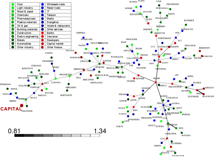
This graph was calculated for sufficiently long duration time, from 2005-01-03 to 2006-03-09, where the worldwide financial crash was still absent DiSo .

We pay our attention mainly for the CAPITAL financial company⁴⁴4The full name of this company is CAPITAL Partners. It is present on the Warsaw Stock Exchange from 20th October 2004. The capital investment in various assets and investment advisement are main purposes of this company activity., which is a suburban company for the most duration time round. However, it becomes a central company for the tree presented in Figure 5 that is, it is a central company for the duration time from 2007-06-01 to 2008-08-12, which already comprises the worldwide financial crash.

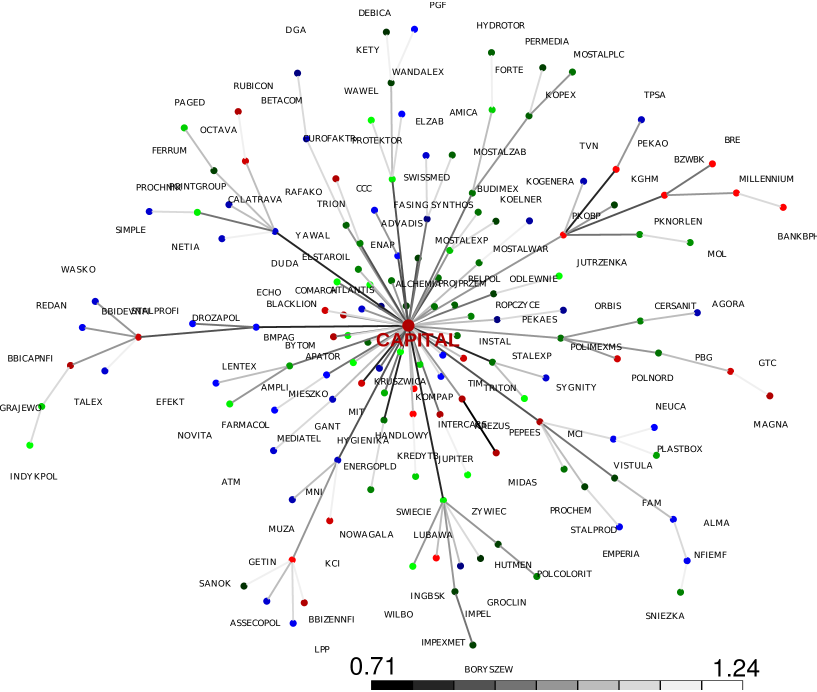
In other words, for the latter duration time the CAPITAL company is represented by the vertex, which has much larger number of edges (or it is of much larger degree) than any other vertex (or company) that is, it becomes a dominated hub (or superhub being a giant component). Notably, the company Salzgitter AG – Stahl und Technologie plays, on the German (Frankfurt) Stock Exchange, the role analogous to the CAPITAL Partners one.

Indeed in the way described above, the transition between two structurally (or topologically) different states of stock exchange is realized. That is, we observed the transition from hierarchical tree (consisting of hierarchy of local stars or hubs) to the superstar like tree (or superhub).

Furthermore, in Figure 6 we compared distributions of vertex degrees for both trees.

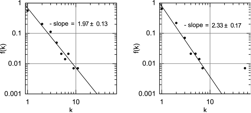
Although these distributions are power–laws, we cannot say that herein we deal with the Albert–Barabási (AB) like complex network with their rule of preferential linking of new vertices AB . This is because for both our trees the power–law exponents are distinctly smaller than 3 (indeed, exponent equals 3 characterizes the AB network), which is a typical observation for many real complex networks DGM . More precisely, the slope (equals $-1.97\mp 0.13$ ) of the lhs plot in Figure 6 also characterizes complex networks of e–mails EMB . The slope (equals $-2.33\mp 0.17$ ) of the rhs plot in this Figure is also characteristic for the complex network of actors (where also superstars are present) WS ; ASBS .

Remarkable that rhs plot in Figure 6 makes possible to consider tree presented in Figure 5 also as a hierarchical MST decorated by a dragon king. Due to our opinion, the appearance of such a dragon king is a signature of a crash.

It seems to be an interesting project to find a proper local dynamics (perhaps nonlinear) for our network. The more so, the single vertex (representing the CAPITAL company) is located far from the straight line (in log-log plot) and can be considered as a temporal outstanding, super-extreme event or a dragon king DSDS ; WGKS ; AJK ; MaSo , which condenses the most amount of edges (or links).

For completeness, the MST was constructed for WSE for the third range of duration time that is, from 2008-07-01 to 2011-02-28, i.e. placed after the worldwide financial crash (cf. Figure 7).

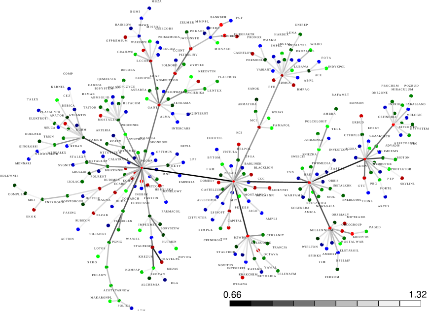
It is interesting that several new hubs appeared while the single superhub (superstar) disappeared (as it became a usual hub). This means that the structure (or topology) of the network is varied during its evolution over the market crash. This is also well confirmed by the plot in Figure 8, where several points (represented large hubs but not superhubs) are placed above the power law. Apparently, this power law is defined by the slope equals $-2.62\mp 0.18$ and also cannot be considered as AB complex network. Rather, it is analogous to the internet, which is characterized by almost the same slope FFF ; CCGJSW .

Above given considerations were confirmed by plots shown in Figures 9 and 10, where well defined absolute minimums at a beginning of 2008 (inside the duration time from 2007-06-01 to 2008-08-12) are clearly shown.

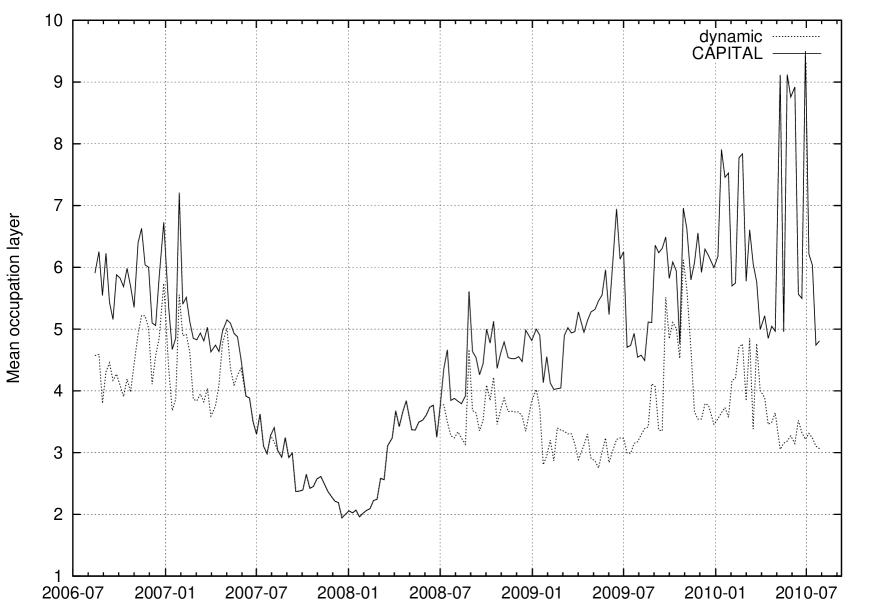
As usual, by the normalized length of the MST tree it is simply understood the average length of the edge (directly) connecting two vertices⁵⁵5Obviously, the edge between two vertices is taken into account if any connection between them exists.. The normalization was chosen so to obtain length equals 1 for pure star like tree. Apparently, this normalized length vs. time has absolute minimum close to 1 at the beginning of 2008 (cf. Figure 9), while for other moments much shallower (local) minimums are observed. Furthermore, by applying the mean occupation layer defined, as usual, by the mean number of subsequent edges connecting a given vertex of a tree with the central vertex (being herein the CAPITAL company), we obtained very similar result (cf. solid line in Figure 10). For comparison, the result based on the other central temporal hubs (having temporary the largest degrees) was also obtained (cf. the dashed curve in Figure 10). This approach is called the dynamic one. Fortunately, all above used approaches give fully consistent results.

The existence of the absolute minimum (shown in Figure 10) for the CAPITAL company and simultaneously, existence of the absolute minimum shown in Figures 9 (to good approximation) at the same moment, confirms the existence of the star like MST structure centered indeed around the CAPITAL company as a superhub.

II.2 Initial conclusions

In this Section we studied the empirical evolving correlated network associated with Warsaw Stock Exchange⁶⁶6We also studied the Franfurt Stock Exchange. Because obtained results are analogous to that found for WSE, we skipped them.. The analytical treatment of such a network is still a challenge.

Our work supplies empirical evidence that there is the dynamic topological (structural) phase transition inside the time range dominated by a crash. Before and after this range superhub disappeared and we observed pure hierarchical MST and hierarchical MST decorated by several hubs (but not superhub), respectively. That is, our results consistently confirm the existence of a dynamic structural phase transitions:

	phase of hierarchical tree $\Rightarrow$ phase of star like tree $\Rightarrow$
	$\displaystyle\mbox{$\Rightarrow$ phase of hierarchical tree decorated by several local star like trees}.$

One of the most significant observation contained in this work comes from plots in Figures 6 and 8. Namely, exponents of all degree distributions are smaller than 3, which means that all variances of vertex degrees diverge⁷⁷7It seems that the degree distribution exponent even smaller than 2 could happened for MST obtained for the duration time from 2005-01-03 to 2006-03-09 (cf. the lhs plot in Figure 4).. This result indicates that herein we deal with criticality that is, the scenario of our network evolution takes place within some scaling region DGM ; DS0 ; BaPo ; HH containing a critical phenomena. Although our situation is more complicated (as power laws here are either decorated by hubs (including the case of a superhub) or governed by exponent slightly smaller than 2), we suppose that phenomenological theory of cooperative phenomena in networks proposed by Goltsev et al. GDM could be a promising first attempt.

Alternative view for our results could consider the superhub phase as a temporal condensate DGM . Hence, we can reformulate above mentioned phase transitions as representing the dynamic transition from excited phase into the condensate and next the transition outside of the condensate again to some excited phase.

We can summarize this work by the conclusion that it seems promising to study in details above considered phase transitions, which yet defines the basis for understanding of a stock market evolution as a whole.

III Systematic analysis of empirical data

III.1 Signals and detrended signals

The systematic analysis of empirical data we perform (as we already indicated in Section I), for the bubbles of WIG, DAX and DJIA indices concerning the recent worldwide financial crisis (cf. Figures 1-3). That is, the bubbles (hossas or booms) represent the left-hand side of the corresponding peaks which seems to be the typical of stock exchanges of small to large capitalization. It is remarkable how awfully similar are shapes of WIG and DAX peaks. This is a generic property of European stock market corresponding peaks.

The bubbles were quite well approximated by our (deterministic) long-term (multi-year) trend (cf. Equation (1.2) in MKRK ). By subtractions this trend from empirical time series (i.e., from the daily time series of indices) we obtained a noisy, at least partially detrended quick-changing signal as a remainder of the bubbles (cf. Figure 11).

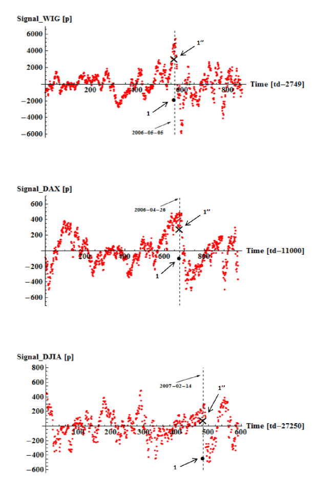
Indeed, this signal is the main subject of our analysis particularly, the most visible downcast ones marked by dashed vertical lines. These objects are located around $566^{th}$ , $676^{th}$ and $483^{rd}$ trading days of the WIG, DAX and DJIA bubbles, respectively. Precisely, these characteristic trading days are the positions of the variance spikes’ centers, well seen in Figure 17. Note that DJIA largest spike appeared only at 2007-02-14 when the subprime market was definitely broken down that is, the latest from these three indices.

III.2 Noise and its distributions

For completeness, besides the signal we analyze its noise (increments), for example, for WIG (cf. Figure 12) from 2004-02-06 to 2007-07-06 that is, for the left side of the peak shown in Figure 1.

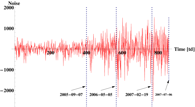
One can observe that before 2005-09-07 the amplitude of the noise is distinctly smaller than that after 2006-05-05 (the region inbetween one can consider as an intermediate one).

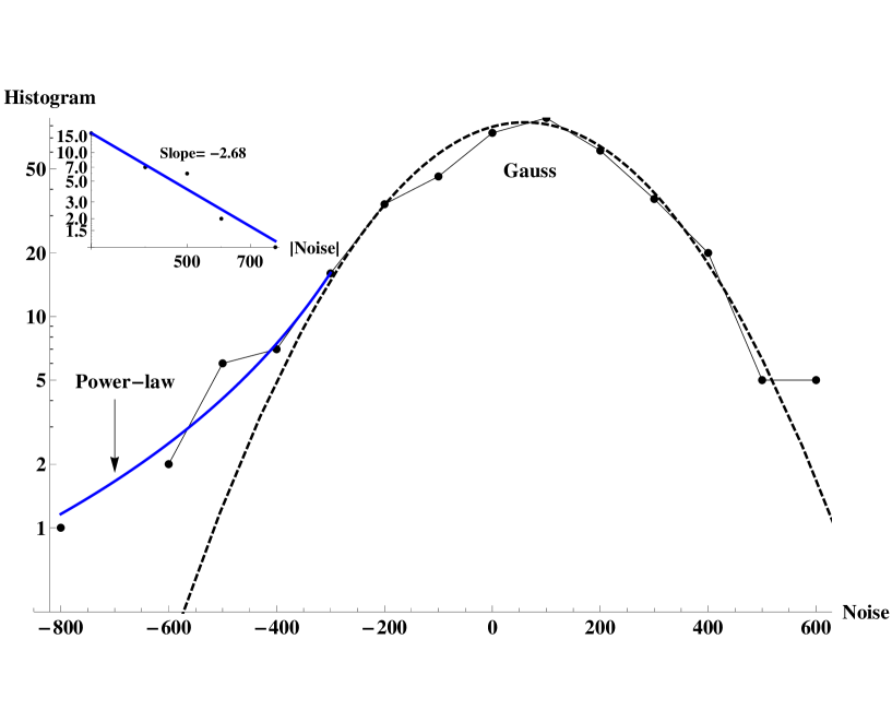
For better insight into the structure of the noise the histograms of the noise were prepared for two above mentioned regions (that is, before and after 2005-09-07). In Figure 13 the semi-logarithmic plot of the histogram for the noise for the first region is presented. As it is seen, it consists of well formed central Gaussian part and poorly formed power-law with slope equals -2.68 for relatively large absolute values of negative increments.

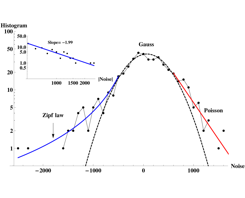
In Figure 14 the analogous histogram was shown for the second region. Again, the central part of the histogram is Gaussian and left part is better formed power-law with slope equals -1.99. However, the right part of the histogram is well fitted by the exponential (Poisson) distribution.

For completeness, in Figure 15 the histogram of the noise of detrended signal for the right part of the peak was shown. As it is seen, the Gaussian distribution satisfactorily fits the empirical data, except few singlets outside the distribution.

To summarize results presented in Figures 13-15 we plotted in Figure 16 the one-sided Lévy exponent $\alpha$ vs. time (counted in months).

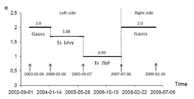
All values of this exponent was obtained by the corresponding fits presented in Figures 13-15. The jump of the exponent $\alpha$ , from the Zipf value before the threshold (marked by the dashed vertical line) to the Gauss one after this threshold, is clearly shown.

Importantly, in Appendix C we proposed a time-dependent distribution of increments in the scaling form (39). That is, we proposed distribution obtained in our earlier work RK (and refs. therein) for the Continuous-time Weierstrass Flights model, where spatio-temporal coupling was used. Hence, we found the searched distribution of increments (independently of any time interval) in the form (43), where $\alpha=-2/\eta$ and $\eta=-2.02$ (as here $\alpha=-0.99$ ). Further in the text we exploit Expression (39) in a way fully consistent with all our empirical data.

III.3 Usual variance of detrended signal

For our three different signals the time dependence of sufficiently sensitive estimators of the usual variance, defined within the moving (or scanning) time window of a one month width (or twenty trading days⁸⁸8Twenty trading days is considered as one trading month keeping Central Bank (riskless) reference return fixed.), is shown in Figure 17. That is, we obtained these estimators by the corresponding separate scannings of empirical time series. These scannings were made by using (mentioned above) time window of the fixed width and also fixed scanning time step (again of one trading month). Indeed, within this window the variance estimator was calculated for each temporal position of the time window.

Notably, the variance estimators of signals suddenly strongly increase in the range of downcasts (marked by circles in Figures 1 - 3), creating local peaks of these estimators in the form of spikes (cf. three plots in Figure 17). The centers of these spikes are indicated in the plots by vertical dashed lines. The existence of the spike is the one of the significant empirical symptom of catastrophic or even critical slowing downs. Further in the text we call these spikes the catastrophic spikes.

Apparently (cf. Figure 17), the catastrophic spikes are preceded by well formed local peaks of variance estimators having much smaller amplitude. This behavior clearly manifests a flickering phenomenon SBBB . This can happen, for instance, if the system enters the intermediate bistable (bifurcation) region placed between two tipping points. Then the system is stochastically moving down and up either between the basins of attraction of two alternative attractors or between attractor and repeller; both possibilities are defined by stable/stable or stable/unstable pairs of equilibrium states. Such a behavior can be also considered as an early-warning indicator. Moreover, the flickering of the variance estimator (although less intensive) together with intermittencies shrinking in time, are observed even for earlier time intervals (cf. the upper plot in Figure 17). This flickering phenomenon is considered in details in Section III.5.

III.4 Accumulative variance of detrended signal

In Figure 18 the accumulative variance (ACV) estimators of our three detrended signals (WIG, DAX, and DJIA) were shown. These variance estimators were presented for the same time ranges as those used in Figure 17. They are much more stable quantities than the usual variance estimators and less sensitive to details of time series, which is a feature useful for study both catastrophic and critical properties.

The ACV estimators show herein that our systems are bimodal ones in the vicinity of the catastrophic spikes. That is, the state characterized by the lower value of the accumulative variance estimator is well separated from the state of the higher value of this estimator. That is, ACV estimator is (almost) constant directly before and after as time $t$ passes the relatively narrow intermediate bistable region where ACV estimator rapidly rises. For instance, for WIG this region extends from about $t_{down}=520$ to $t_{up}=590$ trading days. Indeed, for time earlier than $t=t_{down}$ the system occupies the lower attractor while above $t_{down}$ the ACV estimator sharply increases to the upper attractor. This increase of ACV estimator provides an advance warning that the system approaches a regime shift, being a substantial reorganization of a financial market toward a herden collective or coherent phenomena.

It was shown recently BCS , that the variance estimator increasing near the threshold should be expected in wide range of social and ecological systems with multiple attractors. In this work we empirically prove that also financial markets can obey this feature.

In the subsequent stages we are interested in the time-dependence of the coefficient $AR(1)$ and the lag-1 autocorrelation function, $ACF(1)$ , mainly within the ranges defined by the catastrophic spikes.

III.5 Recovery rate

In Figure 19 was plotted, as a typical behavior, the WIG current signal $x_{t}$ against the preceding signal $x_{t-1}$ .

Two plots of significantly different sets of empirical data were shown there. Each set consists of twenty successive pairs of detrended signal (process) $(x_{t-1},x_{t})$ extended from $t=522$ to $t=541$ trading days (full circles) and from $t=542$ to $t=561$ trading days (inverted triangles), respectively. The slopes of straight lines fitted separately to both data sets give two different values of $AR(1)$ coefficient. That is, these slopes give values of coefficient $AR(1)=1+\lambda$ , where $\lambda$ is a derivative of the nonlinear drift term, $f(x_{t};P)$ (where $P$ is a driving or control parameter), over the signal variable, $x_{t}$ , present in the Langevin Equation (16). This equation is discretized and linearized in the vicinity of the catastrophic bifurcation point (cf. Section B.1). Furthermore, both different values of the shift coefficient $b$ , although relatively small, are well distinguishable in the inset plot.

In Figures 20 and 21 coefficients $AR(1)$ and $-\lambda$ were presented, respectively.

It is remarkable that all our empirical data give $-1<\lambda\leq 0$ . Such a restricted range of $\lambda$ is the crucial result, which is the one of necessary requirement (or signature) of existence the catastrophic bifurcation transition.

Apparently, from fits mentioned above, the larger $AR(1)$ coefficient, almost equals $1.0$ , is present for the latter set of data placed near to the catastrophic bifurcation threshold (marked by the dotted vertical straight line plotted in these figures). For the former set, placed one month earlier, we obtained much lower quantity $AR(1)\approx 0.60$ , as it should be.

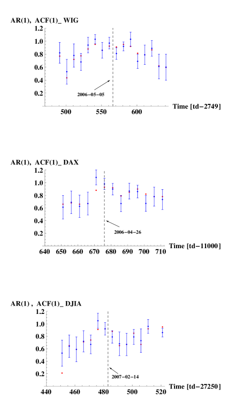
In Section B.2 we proved that both for infinite and finite time series (which in all our cases consists of 20 elements) $ACF(h)$ is expressed by the formula given in the second row in (18). In fact, we study $ACF(1)=AR(1)=1+\lambda$ by the method alternative to that used in Section III.5 to analysis of the coefficient $AR(1)$ . Namely, we applied an usual estimator, $ACF_{EST}(1)$ , of $ACF(1)$ for a given month (which is our time window where $\lambda$ is constant),

\displaystyle ACF_{EST}(1)=\frac{1}{Var(x_{t})}\frac{1}{20}\left[\left(\sum_{t=0}^{19}x_{t}\,x_{t+1}\right)-\frac{1}{20}\left(\sum_{t=0}^{19}x_{t}\right)\left(\sum_{t=0}^{19}x_{t+1}\right)\right].

(1)

Indeed, this estimator is plotted in Figure 20, approaching (to good approximation) its maximal value equals 1.0 in the vicinity of the threshold (marked by the dashed vertical line). This result, together with the corresponding one for coefficient $AR(1)$ , are the basic achievements of our work. The results presented in Figure 21 for recovery rate already follows from them.

Our approach is justified by assuming that $\lambda$ is a piecewise constant function of time, i.e., it is a fixed quantity for each set of twenty data points; the same we assume for the shift coefficient $b$ considered below. Hence, $\lambda$ and $b$ are slowly varying function of time (counted in months) in comparison with process $x_{t}$ (counted in days). They play a crucial role in our considerations.

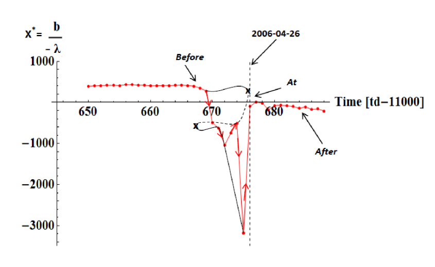
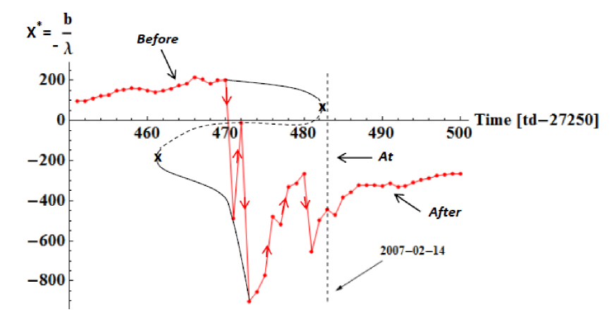
III.6 Empirical catastrophic bifurcation transitions

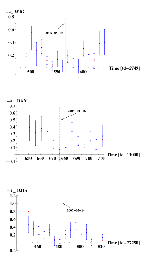
The shift coefficient $b$ relates to recovery rate $\lambda$ and root $x^{*}$ by equality $b=-\lambda x^{*}$ (see the second equation in (16)). Hence, we derived roots $x_{j}^{*},\,j=1^{\prime\prime},1^{\prime},1$ , and successively plotted their dependence on time in Figures 22-24. Sufficiently far from the catastrophic bifurcation threshold the spontaneous (maybe an accidental) reduction of error bars of the curve $x^{*}$ vs. time $t$ is observed together with smoothing out of this curve. The significant jump of this curve is seen only in the nearest vicinity of this threshold. We suppose that both these empirical facts have rather universal character as they are well seen for typical stock markets of small, middle and large capitalization.

The so called, flickering phenomenon (defined already in Section III.3) between stable roots $x_{1^{\prime\prime}}^{*}$ and $x_{1}^{*}$ are well seen on these figures around the negative catastrophic spikes. The flickering phenomenon can mainly appear within the bifurcation region where unstable intermediate state ( $x_{1^{\prime}}^{*}$ ) makes bounce of the system (between the above mentioned stable roots) easier. Indeed, this bounce is able to significantly increase the variance (this effect we discuss in Section B.2). We can consider the flickering phenomenon as a possible precursor of the bifurcation catastrophic transition.

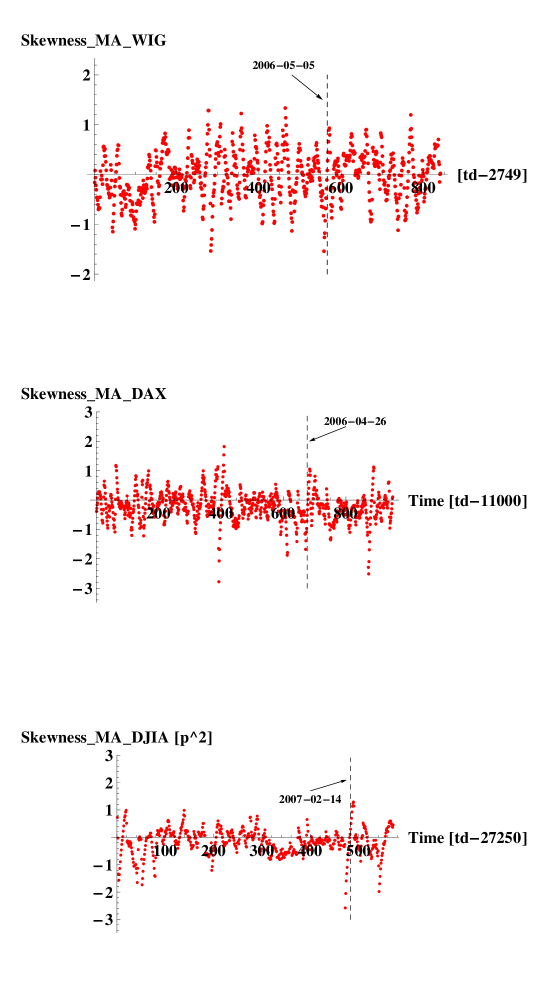
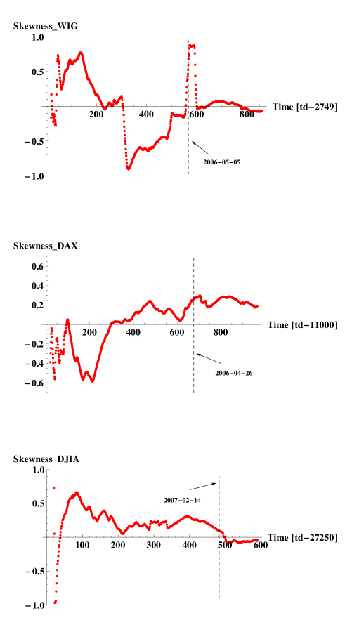
The key results shown in Figures 22-24 constitutes basis for further considerations because they suggest that bistabilities on financial markets can exist.

III.7 Nonlinear indicator: skewness

In Figure 25 the time dependence of the skewness of detrended signal is shown. Relatively large changes in skewness are observed. To verify whether these changes are statistically relevant we calculated a cumulative skewness. This, more stable and less sensitive to unimportant details, quantity was plotted in Figure 26. It presents a strong increase within the range of the spike. This supplies a significant issue that consideration of empirical data within a linearized model, given by the latter equation in (15), is insufficient GJ .

III.8 Periodograms

III.9 Periodograms of signals

It is well known that for the case of finite length time series, the power spectrum ( $PS(\omega)$ , cf. Section B.2) is replaced by its estimator, i.e., by periodogram WAF ; BD ; KS defined as

\displaystyle I(\omega_{j})=T^{-1}\left|\sum_{t=1}^{T}x_{t}\,exp(-i\,t\omega_{j})\right|^{2},\;j=1,2,\ldots,T,

(2)

where $x_{t}$ is a detrended signal, $i$ is an imaginary unit and frequency $\omega_{j}=\frac{2\pi}{T}(j-1)$ (where $j$ we name the frequency number). This enable the observation of a distinct increase of periodogram, $I(\omega_{1}=0)=T^{-1}\mid\sum_{t=1}^{T}x_{t}\mid^{2}$ , that is, its strong increase at $\omega_{1}=0$ in comparison with remained values of the periodogram $I(\omega_{j}),\,j\geq 2$ , (cf. Figure 27; results for DAX and DJIA are analogous).

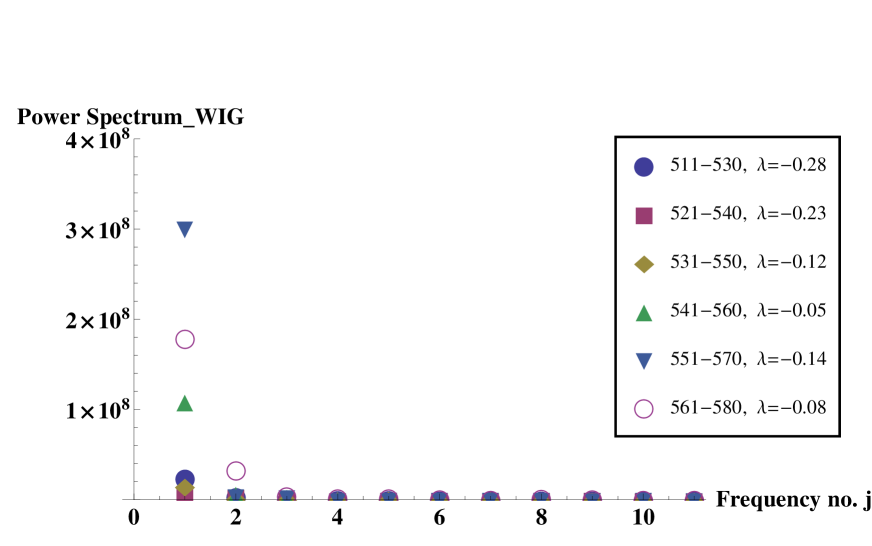
This means that we are able to conclude about reddened of power spectra when discretized time-interval (consisting herein of $T=20$ empirical data points) reach the catastrophic bifurcation transition finally containing it. More precisely, in Figure 27 the last two time intervals (extended from 551 to 570 and 561-580 trading days) contain the catastrophic bifurcation threshold. Therefore, periodograms for these intervals increase at a vanishing frequency $\omega_{1}=0$ , as it was suggested by Formula (4). In fact, the difference between two periodograms at $j=1$ representing inverted triangles and white circles can be considered as some error bar.

Namely, for $\mid\omega\mid\ll 1$ we obtain from Expression (22) that

\displaystyle PS(\omega)\approx-\frac{\lambda\,(2+\lambda)}{\lambda^{2}-(1+\lambda)\,\omega^{2}}\approx-\,\frac{2\lambda}{\lambda^{2}-\omega^{2}},

(3)

where the latter Expression in (3) was obtained at additional condition $\mid\lambda\mid\ll 1$ .

By assuming that $\lambda$ vanishes slower than $\omega$ (at least in the nearest vicinity of the catastrophic bifurcation threshold), we obtain from Equation (3) that

\displaystyle PS(\omega)\approx-\frac{2}{\lambda}.

(4)

Expression (4) says that as system approaches catastrophic bifurcation transition the singularity (which for empirical data manifests by a distinct but finite spike) shifts systematically to lower frequencies as then $\lambda$ vanishes. Indeed, this is well known reddened of the power spectrum. In other words, the significant increase of the peridogram shown by inverted triangle in Figure 27 at $\omega=0$ (or $j=1$ ), is found as time-interval was shifted toward the catastrophic bifurcation transition. This increase is a "finger print" of the catastrophic bifurcation transition.

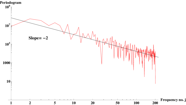
It should be admitted that both empirical periodograms for detrended signals that is, the first one for time series ranging from 1 to 400 (see Figure 28 for details) and the second one from 401 to 859 (see Figure 29 for further details) give (in log-log plot) slopes consistent with distributions shown in plots in Figures 13 and 14 (cf. Appendix C), respectively. These results are also consistent with corresponding ones considered in Section III.10 below.

III.10 Periodograms of noises

The periodogram of the noise (increments) $\Delta x_{t}=x_{t+1}-x_{t}$ has the form analogous to (2), where $x_{t}$ is replaced by $\Delta x_{t}$ and $T$ by $T-1$ . Two characteristic plots of periodograms of noises are presented in Figures 30 and 31.

The result presented in Figure 31 makes possible to estimate the Hurst exponent $H$ by using the Geweke and Porter-Hudak (GPH) method GPH ; RW . According to this method a simple linear regression

\displaystyle\ln I(\omega_{k})=const-(H-0.5)\ln\left(4\sin^{2}(\omega_{k}/2)\right)

(5)

should be valid at low frequencies $\omega_{k},\;k=1,\ldots,K\leq T/2$ .

Several authors suggested that the length $K$ of part of periodogram covered by power law obeys the following inequalities $Int\left[L^{0.2}\right]\leq K\leq Int\left[L^{0.5}\right]$ . In our case (where the length of time series $L=400$ and $K=14$ ) we obtain $K=Int[L^{0.44}]$ in accordance with these inequalities.

Furthermore, from fit of Relation (5) into the empirical data within the range not larger than $K$ we obtain $-2(H-0.5)=-3.02\Longleftrightarrow H=-1.01$ . Recalling that stationary increment-increment correlation function decays in time-lag according to power-law driven by exponent $2(1-H)$ RK , we obtain as a result that the value of this exponent equals 4.02.

On the other side, already simplified approach⁹⁹9The approach is simplified because more refined on-sided Zipf-law should be considered here. gives the consistence between this value of $H$ and exponents supplied by power-laws shown in Figures 14 and 31. This approach is based on the scaling law given by Equations (26) - (28) in RK . Hence, we have

\displaystyle\mbox{Histogram}(\Delta x)\propto\frac{1}{\Delta x^{1-2/\eta}}=\frac{1}{\Delta x^{1.99}},

(6)

where $\eta/2=H=-1/0.99=-1.01$ . This histogram was already applied in Sect. III.2.

As is apparent, few independent approaches (considered in this Section and Section III.2) give the same value of estimator of the Hurst exponent (burdened by statistical errors no greater than $5\%$ ).

IV Qualitative explanation

In this section, we explain how linear and nonlinear indicators (or early warnings) arise when system approaches the regime shift or catastrophic bifurcation transition (threshold). The linear early warnings such as variance, recovery time, reddened power spectra and related quantities can be derived in the frame of linearized time series defined by the latter equation in (15). In contrast, nonlinear indicators (such as a non-vanishing skewness) require an approach based on the nonlinear and asymmetric part of force $f(x;P)$ (present in Equation (9) in Section B) and on its asymmetric potential $U(x;P)$ (defined by Equation (14)), both in the nearest vicinity of the regime shift (cf. plots in Figure 34 concerning the case at the catastrophic bifurcation threshold). This is one of the simplest viewpoint considered, for instance, in article GJ . Following this article it is possible to give herein at least a qualitative explanation based on the mechanical like picture of the ball moving in the potential landscape.

For instance, we consider a schematic snapshot pictorial views of four different modes (states) of the system on the pathway to regime shift (cf. a sequence of the corresponding Figures 32-36). This pathway is defined by dependence $x^{*}=x^{*}(P)$ where driving (hidden) parameter $P$ is, by definition, a monotonically increasing function of time. The point $x^{*}(P)$ is a root of function $f(x;P)$ , see point $1^{\prime\prime}(=x_{1^{\prime\prime}})$ shown in the upper plot in Figure 32, points $1(=x_{1}),\,1^{\prime}(=x_{1^{\prime}}),\,1^{\prime\prime}$ in the upper plot in Figure 33, points $1,\,1^{\prime\prime}$ shown in Figure 34 and point $1$ in Figure 35 as well as a sequence of points $1,\ 1^{\prime}$ and $1^{\prime\prime}$ present in the summary Figure 36. Indeed, any equilibrium state (stable or unstable) of the system originates from Equation (9) as a root of function $f(x;P)$ .

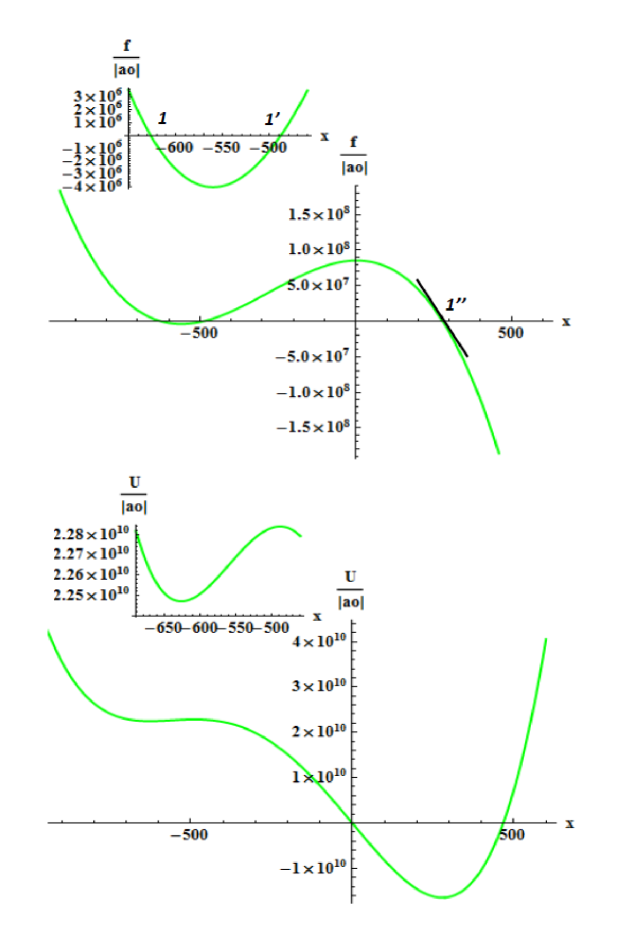
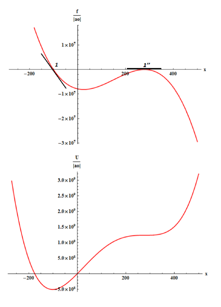
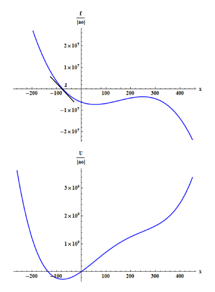
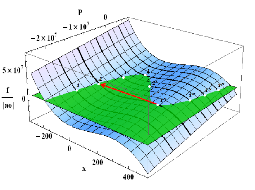
The increase of driving parameter $P$ leads to the shifting of curve $f$ vs. $x$ in the downward direction. This is well seen in the sequence of upper plots. The change of the shape of this curve is also observed although the change is better seen in the corresponding swings of the curve $U$ vs. $x$ shown in lower plots. As a consequence, roots representing stable equilibrium states that is, point $1^{\prime\prime}$ in Figure 32, points $1,\,1^{\prime\prime}$ present in Figures 33 and point $1$ well seen in Figure 35, shift to the left while other, representing unstable equilibrium state that is, point $1^{\prime}$ shown in Figure 33, shifts to the right until disappear. Moreover, point $1^{\prime\prime}$ present in Figure 34 also disappear (cf. next Figure 35). Furthermore, other roots (concerning other catastrophic bifurcation transition) can appear during the system evolution and above given scenario can (at some time) repeats (cf. Figure 38).

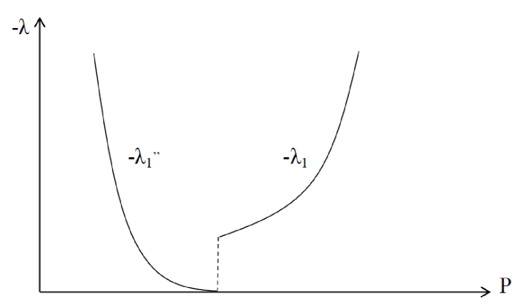
Notably, two segments of the folded backward curve $x^{*}(P)$ containing points $1$ and $1^{\prime\prime}$ (schematically shown in Figure 36), represent stable equilibria, while the third backward segment, containing points $1^{\prime}$ , the unstable one. If the system is driven slightly away from the stable equilibrium it will return to this state with relaxation time $\tau(P)$ (cf. considerations in Section B.1). Otherwise, the system driven from unstable equilibrium will move away (to one of a stable equilibrium). In fact, the backward part of the curve $x^{*}(P)$ represent border or repelling threshold between the corresponding basins of attraction of two alternative stable states (on the lower and upper branches of folded backward curve, marked by solid lines).

In this work we focus mainly on the analysis of stable equilibria. Some of them are tipping points at which a tiny perturbation (spontaneous or systematic) can produce a large sudden transition (marked, e.g. for the second tipping point, by long arrow in Figure 36). It should be noted that only in the vicinity of stable equilibria that is, for points placed on the lower or upper branches of the folded curve, the variance of detrended signal diverges according to power-law (cf. Expression (19) in Section B.2). This is a direct consequence of the critical slowing down, which can be detected well before a critical transition occurring. This divergence can be intuitively understood as follows: as the return time diverges (cf. Sections B.1 and B.4) the impact of a shock does not decay and its accumulating effect increases the variance. Hence, CSD reduces the ability of the system to follow the fluctuations SBBB .

It should be emphasized that observed increase of the skewness within the range of the spike of the variance cannot be explained in the frame of linearized theory. Instead, the nonlinear asymmetric potential in the vicinity of point 1 is needed to have deal with asymmetric distribution (cf. Equation (13)).

V Conclusions

Following the Thomas Lux supposition concerning the possibility of existence of the catastrophic bifurcation transitions on financial markets ThL , we studied several linear and non-linear indicators of such transitions on the stock exchanges of small and middle to large capitalization. All these indicators show self-consistently that thresholds presented in Figures 1 - 18, 20-24, and 26 should be identified as catastrophic bifurcation ones. There is a remarkable surprise that the catastrophic bifurcation threshold itself is so distinct for daily empirical data received from various stock exchanges. As it is seen, such a threshold (related to the kink-antikink pair) was noticed for several months before the global crash. Notably that directly before and after the appearing of the kink-antikink pair the variance of the signal is much less violent.

The basic results of this work was the well established observation that: (i) $\lambda$ is a negative quantity and (ii) recovery rate $\mid\lambda\mid$ vanishes when system approaches the catastrophic bifurcation threshold (cf. Figure 21). This vanishing (together with result mentioned below) permit us to formulate the hypothesis that we deal herein with a catastrophic (but not critical) slowing down. This result is significant the more so as $\lambda$ is a fundamental quantity which constitutes all other linear indicators and partially participates in the non-linear ones.

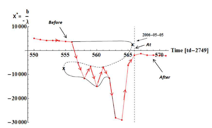
Besides $\lambda$ we found also the shift parameter $b$ (cf. Fig. 19 and, in particular, the inside figure present there). Hence, we were able to plot the empirical trajectory consisting of fixed points $x^{*}$ plotted vs. trading time $t$ and directly observed the catastrophic bifurcation transition preceded by flickering phenomenon (cf. Figures 22-24). This means that the Maxwell construction can be broken here. This is the research highlight of our work. Furthermore, we found that each catastrophic bifurcation transition is directly preceded by singularity, which seems to be a superextreme event.

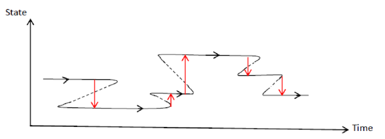
Finally, our study makes possible to formulate two kinds of hypothetical scenarios of financial market evolution shown schematically in Figures 38 and 39. Plot in Figure 38 shows that from time to time evolution of financial market can change abruptly according to subcatastrophic or catastrophic bifurcation transition of different spread between stable regions. However, sometimes the sequence of bifurcated curves presented in Figure 39 can lead (in our case) to ’pitchfork bifurcation’ JJH which arms and stem are stable. Maybe that some of them are so significant that become crashes.

We can conclude that linear and nonlinear indicators used in conjunction in this work provide reliable prediction of regime shift on financial market. However, more systematic verification of relation between the global crash (i.e. the time when hossa is changing to bessa) and preceding it the corresponding catastrophic bifurcation transitions still leave a challenge.

Acknowledgements.

We are grateful Piotr Suffczyński for stimulating discussions. Three of us (T. G., T. R. W., and R. K.) acknowledge partial financial support from the Polish Grant No. 119 awarded within the First Competition of the Committee of Economic Institute, organized by the National Bank of Poland.

Appendix A Detrending procedure

We decided to use herein as a trend the following (deterministic) function of time $t$ :

	$\displaystyle X(\mid t-t_{c}\mid)$	$\displaystyle=$	$\displaystyle(X_{0}-X_{1})E_{\alpha}\left(-\left(\frac{\mid t-t_{c}\mid}{\tau}\right)^{\alpha}\right)$		(7)
		$\displaystyle-$	$\displaystyle X_{1}\cos(\omega\mid t-t_{c}\mid)\cos(\Delta\omega\mid t-t_{c}\mid),\;X_{0},\alpha,\tau,t_{c}>0,$		(7)

valid separately both for the bullish and bearish sides of a given well formed peak. In this work we have $\omega,\,\Delta\omega\ll 1$ (as its is required). If additionally $\Delta\omega\ll\omega$ we deal with a beat. The Mittag-Leffler function $E_{\alpha}(\ldots)$ is defined as follows MK :

\displaystyle E_{\alpha}\left(-\left(\frac{\mid t-t_{c}\mid}{\tau}\right)^{\alpha}\right)=\sum_{n=0}^{\infty}\frac{(-1)^{n}}{\Gamma(1+\alpha n)}\left(\frac{\mid t-t_{c}\mid}{\tau}\right)^{\alpha n},

(8)

where $t_{c}$ is the localization of the turning point (which change market state from bullish to bearish one), $\alpha$ is the shape exponent and $\tau$ plays the role of the relaxation time. The trend function (7) was already derived in our earlier work KK . The parameters and coefficients describing this function for indexes WIG, DAX, and DJIA hossas and bessas were presented in the corresponding tables placed below. The trend function obtained on this way exhibits (as it is required) an unsustainable super-exponential (stretched exponential) growth preceding the speculation-induced crash.

Remarkable that the trend function was derived in the frame of our Rheological Model of Fractional Dynamics of Financial Markets. This model introduces the hypothesis that stock markets response like visco-elastic biopolimer. That is, they are elastic (i.e., immediately response) if an external force impact on a stock market is sufficiently impetuous and they are more like a liquid (plastic) material in the opposite case (of a weak external force). That is, the financial markets can behave as a non-Newtonian liquid.

Notably, among fit parameters and coefficients for a given index (see tables 1 - 12) there exists always at least one which is burdened by large standard deviation. Indeed, this way the system is protected against an arbitrage. Other protection is that time $t_{c}$ (the location of turning point from hossa to bessa) is (to some extend) random.

Table 1: Values of fit parameters of the trend for WIG hossa (

R^{2}=0.9986

)

Parameter	Value	Standard deviation
$t_{c}$	$892\;[td]$	$73\;[td]$
$\tau$	$105\;[td]$	$420\;[td]$
$\alpha$	$0.57$	$0.23$
$\omega$	$0.0041\;[td^{-1}]$	$0.0005\;[td^{-1}]$
$\Delta\omega$	$0.0$	$0.0$

Table 2: Values of fit coefficients of the trend for WIG hossa (

R^{2}=0.9986

)

Parameter	Value [p]	Standard deviation [p]
$X_{0}+X_{1}$	$60081$	$85273$
$X_{1}$	$-8659$	$2352$

Table 3: Values of fit parameters of the trend for WIG bessa (

R^{2}=0.9985

)

Parameter	Value	Standard deviation
$t_{c}$	$810\;[td]$	$0\;[td]$
$\tau$	$272\;[td]$	$20\;[td]$
$\alpha$	$1.562$	$0.025$
$\omega$	$0.0431\;[td^{-1}]$	$0.0005\;[td^{-1}]$
$\Delta\omega$	$0.0065$	$0.0004$

Table 4: Values of fit coefficients of the trend for WIG bessa (

R^{2}=0.9985

)

Parameter	Value [p]	Standard deviation [p]
$X_{0}+X_{1}$	$41963$	$334$
$X_{1}$	$-2528$	$269$

Table 5: Values of fit parameters of the trend for DAX hossa (

R^{2}=0.9985

)

Parameter	Value	Standard deviation
$t_{c}$	$969\;[td]$	$1\;[td]$
$\tau$	$426\;[td]$	$391\;[td]$
$\alpha$	$0.52$	$0.03$
$\omega$	$0.00362\;[td^{-1}]$	$0.00004;[td^{-1}]$
$\Delta\omega$	$0.0065$	$0.0004$

Table 6: Values of fit coefficients of the trend for DAX hossa (

R^{2}=0.9985

)

Parameter	Value [p]	Standard deviation [p]
$X_{0}+X_{1}$	$4698$	$82$
$X_{1}$	$-763$	$35$

Table 7: Values of fit parameters of the trend for DAX bessa (

R^{2}=0.9977

)

Parameter	Value	Standard deviation
$t_{c}$	$968\;[td]$	$0\;[td]$
$\tau$	$426\;[td]$	$72\;[td]$
$\alpha$	$1.12$	$0.03$
$\omega$	$0.0089\;[td^{-1}]$	$0.0001;[td^{-1}]$
$\Delta\omega$	$0.0246$	$0.0001$

Table 8: Values of fit coefficients of the trend for DAX bessa (

R^{2}=0.9977

)

Parameter	Value [p]	Standard deviation [p]
$X_{0}+X_{1}$	$5464$	$70$
$X_{1}$	$-847$	$36$

Table 9: Values of fit parameters of the trend for DJIA hossa (

R^{2}=0.9996

)

Parameter	Value	Standard deviation
$t_{c}$	$627\;[td]$	$3\;[td]$
$\tau$	$333\;[td]$	$38\;[td]$
$\alpha$	$1.29$	$0.02$
$\omega$	$0.0107\;[td^{-1}]$	$0.0002;[td^{-1}]$
$\Delta\omega$	$0.0220$	$0.0002$

Table 10: Values of fit coefficients of the trend for DJIA hossa (

R^{2}=0.9996

)

Parameter	Value [p]	Standard deviation [p]
$X_{0}+X_{1}$	$3486$	$40$
$X_{1}$	$-332$	$28$

Table 11: Values of fit parameters of the trend for DJIA bessa (

R^{2}=0.9971

)

Parameter	Value	Standard deviation
$t_{c}$	$640\;[td]$	$0\;[td]$
$\tau$	$165\;[td]$	$191\;[td]$
$\alpha$	$1.938$	$0.575$
$\omega$	$0.030\;[td^{-1}]$	$0.070;[td^{-1}]$
$\Delta\omega$	$0.040$	$0.070$

Table 12: Values of fit coefficients of the trend for DJIA bessa (

R^{2}=0.9971

)

Parameter	Value [p]	Standard deviation [p]
$X_{0}+X_{1}$	$4010$	$110$
$X_{1}$	$-866$	$81$

Appendix B Linear indicators of a critical slowing down from bifurcation point of view

In this section we consider linear indicators of the critical slowing down or regime shift such as a variance, recovery time and rate as well as reddened power spectra. The nonlinear indicator is defined by an asymmetric skewness.

Let us suppose that detrended time-dependent signal, $x_{t}\stackrel{{\scriptstyle\rm def.}}{{=}}X(t)-\mbox{Trend}(t)$ , obeys the first order difference equation of the stochastic dynamics

\displaystyle x_{t+1}-x_{t}=f(x_{t};P)+\eta_{\,t}

(9)

where $P$ is a driving (control, in general vector) parameter and the additive noise $\eta_{\,t},\;t=0,1,2,\ldots,$ is a $\delta$ -correlated¹⁰¹⁰10Herein, the notation $\delta$ means the Kronecker delta while $t$ numbers, in our case, trading days within a given trading month (which consists of 20 trading days). The trading month is our time window where $\lambda$ is constant. $(0,\sigma^{2})$ random variable. In the upper plots in Figures 33-35 the schematic behaviors of function $f$ vs. variable $x$ were shown for different values of parameter $P$ . In the comprehensive Figure 36 these dependences are collected in the form of the three-dimensional plot. It is seen that function $f$ could be, for instance, a third-order polynomial having $P$ -dependent coefficients (cf. Section B.5).

B.0.1 Continuous-time formulation

Simultaneously, we consider the differential formulation of Equation (9), which basic ingredient is the Langevin dynamics DS0 , NGvK . This differential formulation takes the form of the massless stochastic dynamic equation

\displaystyle\frac{\partial x_{t}}{\partial t}=-\frac{\partial U(x_{t};P)}{\partial x_{t}}+\eta_{t},

(10)

where $U$ plays the role of a mechanic potential while $\eta_{t}$ of a stochastic force. This equation is equivalent to the quasi-linear (according to van Kampen terminology NGvK ) Fokker-Planck equation

\displaystyle\frac{\partial{\cal P}(x,t)}{\partial t}=-\frac{\partial j(x,t)}{\partial x}

(11)

which has the form of continuity equation (a conservation law) for probability density ${\cal P}(x,t)$ , where the current density is given by constitutive equation

\displaystyle j(x,t)=f(x;P)\,{\cal P}(x,t)-\frac{\sigma^{2}}{2}\frac{\partial{\cal P}(x,t)}{\partial x}.

(12)

The equilbrium solution of Equation (11) (obtained directly from requirement that no current is present in the system, i.e. by assuming that $j(x,t)=0$ in Equation (12)) is given by

\displaystyle{\cal P}^{eq}(x)\sim\frac{2}{\sigma^{2}}\exp\left(-\frac{2}{\sigma^{2}}\,U(x;P)\right),

(13)

where potential $U(x;P)$ already appeared in Equation (10), while

\displaystyle f(x;P)=-\frac{\partial U(x;P)}{\partial x}

(14)

is (in this terminology) a mechanical force. Both Formulas (13) and (14) play an important role in our explanations. That is, a positive asymmetry of the potential $U$ in the vicinity of fixed point $1^{\prime\prime}$ at the bifurcation threshold (cf. the middle plot in Figure 34) could be a cause of large positive cumulative skewness in this vicinity.

Taking into account the spirit of the Time Dependent Ginzburg-Landau theory of phase transition DS0 , we can assume that potential $U(x;P)$ is a polynomial of the fourth order (hence, force $f$ is a polynomial of the third order, cf. Section B.5). It is a technical task to establish required relations between coefficients of the polynomial when system tends to the critical bifurcation.

In this Section our considerations consist of few stages: (i) the analysis of the linear stability, (ii) the analysis of the non-equilibrium critical dynamics next to a catastrophic bifurcation, (iii) consideration, for instance, the case of polynomial form of $f$ , and (iv) derivation of the useful properties of the first order autoregressive time series.

B.1 Analysis of the linear stability

In this stage we study, in fact, the linear stability of an equilibrium that is, we consider the relaxation of the system which was slightly knocked out from its equilibrium CW . The equilibrium of the system is defined by the root (or fixed point) of function $f$ at corresponding value of the driving parameter. This definition does not exclude some fluctuations supplied by noise $\eta$ . For instance, in Figure 33 the third root is placed at $x=x_{1^{\prime\prime}}^{*}(P_{1^{\prime\prime}})$ . Indeed, our expansion is made in this root and extended, herein, only to the nearest (linear) surroundings. Moreover, we assume that this root is located next to the catastrophic bifurcation point (cf. Figures 33 and 34).

The linear expansion of $f$ , e.g. at fixed point $1^{\prime\prime}$ , gives

	$\displaystyle y_{t+1}-y_{t}$	$\displaystyle=$	$\displaystyle f(x_{1^{\prime\prime}}^{*}(P_{1^{\prime\prime}});P_{1^{\prime\prime}})+\lambda\,y_{t}+\eta_{\,t}=\lambda\,y_{t}+\eta_{\,t}$		(15)
		$\displaystyle\Leftrightarrow$	$\displaystyle y_{t+1}=(1+\lambda)\,y_{t}+\eta_{\,t}$		(15)

as, by definition of a root, $f(x_{1^{\prime\prime}}^{*}(P_{1^{\prime\prime}});P_{1^{\prime\prime}})$ vanishes Herein, we used the notation: (i) for the displacement from an equilibrium¹¹¹¹11The set of variables $y_{t},\;t=0,1,2,\ldots,$ is also called the first order autoregressive time series. or the (unnormalized) order parameter $y_{t}=x_{t}-x_{1^{\prime\prime}}^{*}(P_{1^{\prime\prime}})\,,\;\;t=0,1,2,\ldots,$ and (ii) for rate $\lambda(P)=\frac{\partial f(x;P)}{\partial x}\mid_{x=x^{*}(P)}$ .

The latter equation in (15), rewritten in the form

\displaystyle x_{t+1}=(1+\lambda)\,x_{t}+b+\eta_{\,t},\;b=-\lambda\,x_{1^{\prime\prime}}^{*}

(16)

makes possible to obtain $\lambda$ and $x_{1^{\prime\prime}}^{*}$ from the fit to empirical data, such as shown in Figure 19. The related quantities were presented in Figures 20-24. However, to make such a fit we assume that coefficients $\lambda$ and $b$ are utmost a slowly varying function of time. Moreover, we assume that they are piecewise functions of time.

The solution of Equation (15) is

\displaystyle y_{t}=(1+\lambda)^{t}y_{0}+(1+\lambda)^{t-1}\sum_{\tau=0}^{t-1}\eta_{\tau}(1+\lambda)^{-\tau}\approx\exp(\lambda t)\left[y_{0}+\int_{0}^{t}\eta_{\tau}\exp(-\lambda\tau)d\tau\right],

(17)

where the first equality is valid for $t\geq 1$ . The second equality in (17) has an exponential form because we confined our considerations only to the case $\mid\lambda\mid\ll 1$ and $t\gg 1$ that is, to the nearest vicinity of the threshold for sufficiently long time. However, in all our calculations we did not include the flickering phenomenon, considering only the nearest vicinity of an equilibrium point (stable or unstable). We suppose that by taking into account this phenomenon we could obtain the significant increase of the variance within the bifurcation region.

>From Equation (17) follows that given equilibrium state is stable if¹²¹²12We observed that for our empirical data always inequality $-1<\lambda<0$ is obeyed. $-2<\lambda<0$ otherwise, it is unstable. Hence, e.g. points $1$ and $1^{\prime\prime}$ in Figure 33 define stable equilibria. In general, stable equilibrium points (or fixed points) are placed on the solid segments of the folded backward curves, while unstable ones are placed on the dashed-dotted segment (cf. all bottom plots in Figures 33-35 and plot in Figure 36).

For the stable equilibrium the relaxation (recovery or return) time $\tau(P)=1/\mid\lambda(P)\mid$ is well defined that is it is a positive quantity. Particularly interesting are stable equilibrium points $x_{1}^{*}$ and $x_{1^{\prime\prime}}^{*}$ shown in Figure 34 as they are border points of two corresponding bifurcation regions (attraction basins) therefore called the catastrophic bifurcation points (or tipping points). They are the most significant states of the system considered in this work.

B.2 Generic properties of the first order autoregressive time series

It is well known WAF ; BD that particularly useful quantities, i.e. variance, covariance and autocorrelation function as well as power spectrum, are related. We calculate them by exploiting an exact solution given by the first equality in (17).

Firstly, we calculate the covariance,

$\displaystyle Cov(y_{t}\,y_{t+h})$	$\displaystyle=$	$\displaystyle\left<y_{t}\,y_{t+h}\right>-\left<y_{t}\right>\left<y_{t+h}\right>=(1+\lambda)^{\mid h\mid}\,Var(y_{t})=$
$\displaystyle Cov(x_{t}\,x_{t+h})$	$\displaystyle=$	$\displaystyle(1+\lambda)^{\mid h\mid}\,Var(x_{t})$	(18)
	$\displaystyle\Leftrightarrow$	$\displaystyle ACF(h)=\frac{Cov(y_{t}\,y_{t+h})}{Var(y_{\,t})}=\frac{Cov(x_{t}\,x_{t+h})}{Var(x_{\,t})}=(1+\lambda)^{\mid h\mid}$
	$\displaystyle\Rightarrow$	$\displaystyle ACF(h)\approx\exp(\lambda\mid h\mid),\;h=0,\pm 1,\pm 2,\ldots,$

where $\lambda$ is expressed by Equation (25) and the variance $Var(y_{t})$ is given (after straightforward calculations) by the significant formula

\displaystyle Var(y_{\,t})=\left<y_{t}^{2}\right>-\left<y_{t}\right>^{2}=Var(x_{\,t})=Var(y_{0})(1+\lambda)^{2t}-\frac{1}{\lambda(2+\lambda)}\left[1-(1+\lambda)^{2t}\right]\sigma^{2},

(19)

where $Var(y_{t})=Var(x_{t})$ and notation $\left<\ldots\right>$ denotes an average over the noise and the initial condition (within the statistical ensemble of solutions $y_{t}$ ). The latter equality in (18) is obeyed for $\mid\lambda\mid\ll 1$ . Therefore, it further simplifies into the form

\displaystyle Var(y_{\,t})\approx Var(y_{0})(1+2\lambda t)+t\sigma^{2}\approx Var(y_{0})+\sigma^{2}t,

(20)

where the latter approximate equality was obtained for $2t\ll\mid\lambda\mid^{-1}$ . We suppose that by taking into account the flickering phenomenon we could obtain the significant increase of the variance within the bifurcation region. However, the analytical calculation of such a variance requires the solution of nonlinear Equation (9) for $f$ given by the polynomial (27), which is still a challenge.

The coefficient $1+\lambda$ (present in (18)) is the lag-1 autocorrelation function, which can be find directly from empirical data (cf. Fig. 20). Apparently, it does not depend on the variance.

Now, as we have an exact simple formula for the stationary autocorrelation function, $ACF(h)$ , we can obtain power spectrum $PS(\omega)$ in an exact analytical form. Namely, from the Wiener-Khinchine theorem KTH we have

	$\displaystyle PS(\omega)$	$\displaystyle=$	$\displaystyle\lim_{H\rightarrow\infty}\sum_{h=-H}^{H}ACF(h)\,\exp(-i\,h\,\omega)=\lim_{H\rightarrow\infty}\sum_{h=-H}^{H}(1+\lambda)^{\mid h\mid}\,\exp(-i\,h\,\omega)$		(21)
		$\displaystyle=$	$\displaystyle-\lim_{H\rightarrow\infty}\frac{\lambda(2+\lambda)-2(1+\lambda)^{H}(1+\lambda-\cos(\omega))}{2+\lambda(2+\lambda)-2(1+\lambda)\cos(\omega)}.$		(21)

Obviously, for $-1<\lambda<0$ (which is our case) the term containing factor $(1+\lambda)^{H}$ in the numerator vanishes. Hence, we obtain a useful formula

\displaystyle PS(\omega)=-\frac{\lambda(2+\lambda)}{2+\lambda(2+\lambda)-2(1+\lambda)\cos(\omega)}.

(22)

For vanishing $p_{j}$ the variance and covariance diverge according to power-law while autocorrelation function tends then to $1$ . Besides, all odd moments of variable $y_{t}$ vanish. Hence and from Equation (19) we find that in the frame of linear theory the skewness also vanishes.

Furthermore, it can be easily verified (again by using solution (17)) that the excess kurtosis vanishes if variables $y_{0}$ and $\eta_{\,t}$ are drawn from some Gaussian distributions. That is, in the frame of the linear theory (i.e. in the vicinity of the threshold) the distribution of variable $y_{t}$ is the Gaussian, which has the variance given by Expression (19) and centered around the mean value $\left<y_{t}\right>=y_{0}(1+\lambda)^{t}$ .

The above given considerations clearly show that indeed $ACF(1)$ or $AR(1)$ coefficient is a basic quantity to study the catastrophic bifurcation, possible for direct determination from empirical data.

B.3 Nonlinear time series analysis

As linear term in the linear time series can be relatively easy masked by the noise term, we expanded $f$ in Expression (9) one step further up to the quadratic term (see also Equation (15)). Hence, we deal with the nonlinear time series. For time series of this type several methods were developed to determine the level of the noise and to make the noise reduced. KS .

B.4 Catastrophic dynamics next to catastrophic bifurcation transition

In the second stage, we more subtle consider the non-equilibrium dynamics in the vicinity of particular equilibrium (fixed) points CW . That is, the dynamics next to catastrophic bifurcation point is considered herein.

Let us make the Taylor expansion at point $x_{j}^{*}(P_{j})$ :

\displaystyle f(x;P)=f(x_{j}^{*}(P_{j})+y_{j};P_{j}+p_{j})=\beta\,p_{j}+\alpha\,y_{j}^{2}+\ldots,

(23)

herein $j=1^{\prime\prime}$ means the only catastrophic bifurcation point, i.e., the catastrophic point placed on the catastrophic bifurcation curve (cf. Figure 36). For sufficiently small $\mid p_{j}\mid$ and $\mid y_{j}\mid$ only first two terms in (23) play an essential role. We used the following notation: for the displacement from catastrophic bifurcation point $y_{j}=x-x_{j}^{*}(P_{j})$ , negative parameter’s deviation $p_{j}=P-P_{j}$ , negative coefficient $\beta=\frac{\partial f(x;P)}{\partial P}\mid_{x=x_{j}^{*}(P_{j}),\,P=P_{j}}$ and for negative coefficient $\alpha=\frac{1}{2}\frac{\partial^{2}f(x;P)}{\partial x^{2}}\mid_{x=x_{j}^{*}(P_{j}),\,P=P_{j}}$ . Note that the sign of each quantity can be easily recognized by comparing curves $f(x)$ vs. $x$ plotted in Figure 36. We used also helpful properties: $f(x_{j}^{*}(P_{j});P_{j})=0$ and $\lambda(P_{j})=0$ (cf. Figure 34 and the catastrophic curve in Figure 36), where the former defines a fixed point while the latter the local maximum at the catastrophic bifurcation point. Due to these properties we get below the searched scaling relations.

By substituting in Equation (23) variable $x=x^{*}(P)$ , we get the scaling relation (as the left-hand side of (23) vanishes then)

\displaystyle y_{j}^{*}=\pm\left[-\left(\frac{\beta\,p_{j}}{\alpha}\right)\right]^{\mu},

(24)

where displacement $y_{j}^{*}=x^{*}(P)-x_{j}^{*}(P_{j})$ is, in this case, a positive quantity (therefore, sign ’+’ standig outside the square brackets should be taken into account) while exponent $\mu=1/2$ plays the role of the critical index (or citical exponent).

The relation (24) shows that the displacement vanishes according to the power-law, when system reaches a catastrophic bifurcation point. This is a signature of phase transition; in our case the discontinuous one that is, the first-order phase transition.

Moreover, from Equations (23), (24) and definition of $\lambda$ we also obtain¹³¹³13Formula (25) was derived from (23) by making the derivative over $x$ variable of its both sides at $x=x^{*}(P)$ . a significant scaling relation

\displaystyle\lambda=2\alpha\,y_{j}^{*}=\pm 2\alpha\left[-\left(\frac{\beta\,p_{j}}{\alpha}\right)\right]^{\mu}.

(25)

The plus sign in the second equality in above equation (outside square brackets) defines the stable equilibrium (as then $\lambda$ is negative), which is our case ( $j=1^{\prime\prime}$ ). The relation (25) shows that rate $\lambda$ also vanishes according to power-law when system reaches a catastrophic bifurcation point, which is a succeeding signature of phase transition. Nevertheless, there is a challenge how $\lambda$ scales with time when it is closed to the transition instant.

B.5 Simplest example: approximation of force $f$ by the third-order polynomial

Let us assume that potential $U$ , present in Eq. (14), is defined by the fourth-order polynomial

\displaystyle U(x;P)=A_{0}x^{4}+A_{1}x^{3}+A_{2}x^{2}+A_{3}x+A_{4},

(26)

where $A_{j},\,j=0,1,\ldots,4$ , are its real coefficients somehow related to (combined) parameter $P$ ; this relation is considered further in this section. According to Eq. (14), force $f$ is a polynomial of one order of magnitude lower

\displaystyle f(x;P)=a_{0}x^{3}+a_{1}x^{2}+a_{2}x+a_{3},

(27)

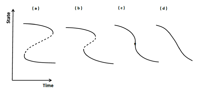
where coefficients $a_{4-j}=-j\,A_{4-j},\,j=1,\ldots,4$ and herein we assume $a_{0}<0$ as it is indicated by empirical data. Below, we consider three characteristic cases: (a) the catastrophic bifurcation transition, (b) the transition before the catastrophic bifurcation transition, and (c) the transition after it. For instance, we consider situations (common for all three cases), where smallest root of polynomial (27) is negative. That is, we consider situations presented in Figures 22 (and placed on the left-hand side of the threshold marked by the straight vertical dashed line) and also 23, where the latter is our working example.

The generic aim of this section is to express coefficients of polynomial (27) in terms of roots of this polynomial.

B.5.1 Case of the catastrophic bifurcation transition

Let us focus on the case (a) (presented in Figure 34) concerning the catastrophic bifurcation transition. This means that coefficients $a_{j},\,j=0,\ldots,3$ , make such a parametrisation, which gives curve $f(x;P)$ vs. $x$ indeed in the form shown in Figure 34 (we relate these coefficients to parameter $P$ at the end of this section).

Now, we can define the goals of this case. There are as follows:

(i)

the derivation of the roots $x_{1}^{*}$ and $x_{1^{\prime\prime}}^{*}$ of polynomial (27) and hence calculation, for instance, the catastrophic bifurcation jump, $\Delta x_{1^{\prime\prime},1}^{*}=x_{1}^{*}-x_{1^{\prime\prime}}^{*}$ , as a function of polynomial coefficients and
(ii)

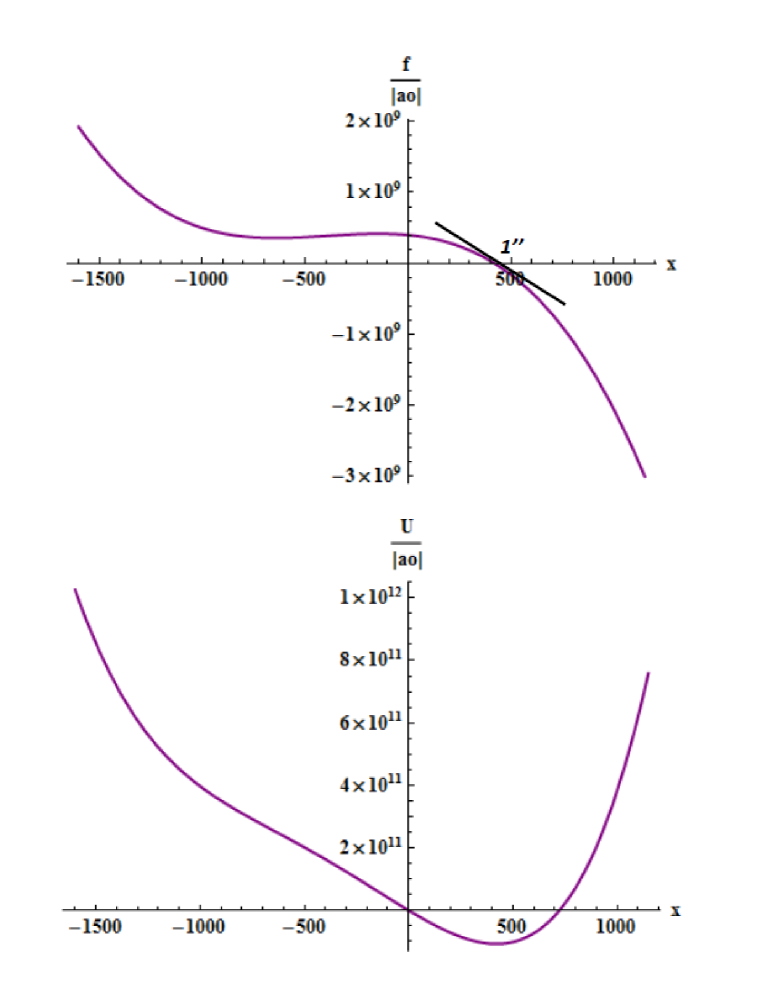
the solution of the inverse problem that is, the derivation of relative parameters $a_{1}/a_{0},\,a_{2}/a_{0}$ and $a_{3}/a_{0}$ by means of roots $x_{1}^{*}$ and $x_{1^{\prime\prime}}^{*}$ , which can be found from empirical data (cf. Figures 22-24 in Section III.5).

Notably, the catastrophic bifurcation transition $1^{\prime\prime}\Rightarrow 1$ (cf. the upper plot in Figure 34) begins at point $1^{\prime\prime}$ , which is not only the largest twofold root of polynomial $f$ but also it is its local maximum that is, it is an inflection point on curve $U$ vs. $x$ (cf. both plots in Figure 34). Hence,

\displaystyle\frac{\partial f(x;P)}{\partial x}\mid_{x=x_{0},\,x_{1^{\prime\prime}}^{*}}\,=0\Leftrightarrow 3\,x_{0,1^{\prime\prime}}^{*\,2}+2\,\frac{a_{1}}{a_{0}}\,x_{0,1^{\prime\prime}}^{*}+\frac{a_{2}}{a_{0}}=0,

(28)

where $0(=x_{0})$ is the first inflection point on curve $U$ vs. $x$ (see again the lower plot in Figure 34) and it is the local minimum of curve $f$ vs. $x$ (see again the upper plot in Figure 34).

>From Equation (28) we obtain

\displaystyle x_{0,1^{\prime\prime}}^{*}=x_{ip}\mp\frac{1}{3}\,\sqrt{D},\,\,D\stackrel{{\scriptstyle\rm def.}}{{=}}\left(\frac{a_{1}}{a_{0}}\right)^{2}-3\,\frac{a_{2}}{a_{0}},

(29)

where sign $-$ concerns minimum $x_{0}^{*}$ , sign $+$ concerns root $x_{1^{\prime\prime}}^{*}$ , while

\displaystyle x_{ip}=-\frac{1}{3}\frac{a_{1}}{a_{0}},

(30)

and we assumed $D>0$ as two real roots of Eq. (28) should exist.

We can easily derive (from vanishing of the second derivative $f$ over $x$ ) that $x_{ip}$ , given by Eq. (30), is the inflection point (cf. the upper plot in Figure 34),

\displaystyle\frac{\partial^{2}f(x;P)}{\partial x^{2}}\mid_{x=x_{ip}}\,=0\Rightarrow x_{ip}=-\frac{1}{3}\frac{a_{1}}{a_{0}}.

(31)

As it follows from Equation (29), both extremes $x_{0}^{*}$ and $x_{1^{\prime\prime}}^{*}$ are located symmetrically on either sides of the inflection point $x_{ip}$ that is, minimum $x_{0}^{*}$ is placed on the left-hand side and $x_{1^{\prime\prime}}^{*}$ on the right-hand side.

By the way, from Equation (28) and definition of coefficient $\alpha$ (given in Section B.4) follow that

\displaystyle\alpha=\frac{1}{2}\left(6x_{1^{\prime\prime}}+2\,\frac{a_{1}}{a_{0}}\right)=-\sqrt{D}.

(32)

We can postulate the complementary properties of coefficients and roots suggested by the empirical data points and corresponding backward folded hypothetical curve shown, for instance, in Figure 23, that is

(i)

we assume inequalities for the roots $x_{1}^{*}<0$ and $x_{1^{\prime\prime}}^{*}>0$ ,
(ii)

the root $x_{1^{\prime\prime}}^{*}$ is a twofold one of polynomial (27), where local maximum of this polynomial is located.

>From item (ii) and by looking for such values of variable $x$ and parameter $P$ for which $f(x;P)$ vanishes in Equation (27), we easily obtain (with help of Eq. (29)) the third root

\displaystyle x_{1}^{*}=x_{ip}-\frac{2}{3}\,\sqrt{D}.

(33)

>From Equations (29), (32) and (33) we get the catastrophic bifurcation jump

\displaystyle\Delta x_{1^{\prime\prime},1}^{*}=-\sqrt{D}=\alpha,

(34)

being function of only two relative parameters $a_{1}/a_{0}$ and $a_{2}/a_{0}$ . This equation gives significant interpretation of parameter $\alpha$ making possible to easily detect it from empirical plots presented in Figures 22 - 24.

>From Egs. (29), (31) and (33) we easily find the solution of the inverse problem in the form,

	$\displaystyle\frac{a_{1}}{a_{0}}=-(2x_{1^{\prime\prime}}^{}+x_{1}^{})\leq 0,$
	$\displaystyle\frac{a_{2}}{a_{0}}=x_{1^{\prime\prime}}^{}\left(x_{1^{\prime\prime}}^{}+2x_{1}^{*}\right)\geq 0,$		(35)

together with the constraint for the relative free parameter

\displaystyle\frac{a_{3}}{a_{0}}=-x_{1}^{*}\,(x_{1^{\prime\prime}}^{*})^{2}\geq 0;

(36)

the latter relation makes the above procedure self-consistent. The above given three inequalities were suggested by empirical data. Following for the data we can assume helpful inequalities: $a_{1}>0,\,a_{2}\leq 0,\,a_{3}<0$ .

Apparently, having tipping points $x_{1}^{*}$ and $x_{1^{\prime\prime}}^{*}$ , taken from empirical data, we can obtain searched relative parameters $a_{1}/a_{0},\,a_{2}/a_{0}$ and $a_{3}/a_{0}$ . Here, we have $x_{1}^{*}=-101.17$ and $x_{1^{\prime\prime}}^{*}=278.92$ which gives $a_{1}/a_{0}=-456.67,\,a_{2}/a_{0}=21359.70$ and $a_{3}/a_{0}=7.87066\times 10^{6}$ .

Notably, the combined parameter $P$ consists of only two independent components, e.g., $a_{1}/a_{0}$ and $a_{2}/a_{0}$ . The first component could be, for example, the volume averaged over month while the second component could be the basic rate of the central bank (which is, obviously, a piecewise function of time counted in month scale). We can say that two components of combined parameter $P$ are already sufficient to perform some simulations at catastrophic transition.

Furthermore, the schematic bottom plots shown in Figures 33-36 tacitly assumed that combined parameter $P$ monotonically depends on time (counted in month time scale) at least in the vicinity of BCT.

B.5.2 Case before the catastrophic bifurcation transition

The case considered here (i.e., the case represented by Figure 33) is a generalization of the one discussed in Section B.5.1. That is, we consider variable $x$ placed inside the bifurcation region, where three different real roots exist (cf. backward folded curves shown in Figures 22 - 24 and schematically shown in Figure 36).

The goal of this section is analogous to that considered in Section B.5.1, i.e., to find coefficients of polynomial (27) by using its roots found from empirical data (shown in the above mentioned figures). By assuming that polynomial (27) has three real different roots we obtain, by comparing Eq. (27) with its multiplicative form $f(x;P)=\left(x-x_{1}^{*}\right)\left(x-x_{1^{\prime}}^{*}\right)\left(x-x_{1^{\prime\prime}}^{*}\right)$ , the searched relations for coefficients of the polynomial

	$\displaystyle\frac{a_{1}}{a_{0}}=-(x_{1^{\prime\prime}}^{}+x_{1^{\prime}}^{}+x_{1}^{*}),$
	$\displaystyle\frac{a_{2}}{a_{0}}=x_{1^{\prime}}^{}x_{1^{\prime\prime}}^{}+x_{1}^{}x_{1^{\prime\prime}}^{}+x_{1}^{}x_{1^{\prime}}^{},$
	$\displaystyle\frac{a_{3}}{a_{0}}=-x_{1}^{}\,x_{1^{\prime}}^{}\,x_{1^{\prime\prime}}^{*}.$		(37)

Apparently, above equations are generalization of the corresponding Eqs. (35) and (36), as we obtain the latter equations by setting in Eqs. (37) $x_{1^{\prime}}^{*}=x_{1^{\prime\prime}}^{*}$ .

Notably, Figure 33 was constructed by using coefficients obtained from Eqs. (37) by introducing into their right-hand sides the following empirical values of roots: $x_{1}^{*}=278.92,\,x_{1^{\prime}}^{*}=-488.308,\,x_{1^{\prime\prime}}^{*}=-626.473$ , taken, for instance, from the backward folded curve shown in Figure 23. According to (37), this leads to $a_{1}/a_{0}=835.861,\,a_{2}/a_{0}=-5022.94,\,a_{3}/a_{0}=-8.53249\times 10^{8}$ .

B.5.3 Case after the catastrophic bifurcation transition

For this case (represented by Figure 35) we have insufficient empirical data for unique solution as only single real root $x_{1}^{*}$ we can find from them (roots $x_{1^{\prime}}^{*}$ and $x_{1^{\prime\prime}}^{*}$ are the complex conjugated). Hence, we deal only with a single relation between coefficients of polynomial

\displaystyle f(x_{1}^{*};P)=-\left(x_{1}^{*}\right)^{3}-\frac{a_{1}}{a_{0}}\left(x_{1}^{*}\right)^{2}-x_{1}^{*}\frac{a_{2}}{a_{0}}-\frac{a_{3}}{a_{0}}=0,

(38)

which makes the ratio of parameters (e.g., $a_{1}/a_{0}$ ) dependent on other two ratios (herein, on $a_{2}/a_{0}$ and $a_{3}/a_{0}$ ). For instance, in Figure 35 we show plots for root $x_{1}^{*}=-75.3875$ as well as ratios of parameters $a_{3}/a_{0}=6.1682\times 10^{6},\,a_{2}/a_{0}=41709.50$ and $a_{1}/a_{0}=-456.67$ .

With analogous situation we deal if $x$ is placed before CBT and outside of the bifurcation region. Then, we deal again with a single real root, here $x_{1^{\prime\prime}}^{*}=421.009$ , while roots $x_{1}$ and $x_{1^{\prime}}^{*}$ are complex conjugated. In Figure 33 we show plots for ratios of parameters $a_{3}/a_{0}=-4.00948\times 10^{8},\,a_{2}/a_{0}=278390$ and $a_{1}/a_{0}=1179.81$ .

Finally one can state, that the approach developed in Sections B.5.1 - B.5.3 is sufficiently flexible that is, can be reformulated for the situation where the smallest root of Eq. (27), $x_{1}^{*}$ , become positive. Then, obviously, signs and values of coefficients $a_{0},\,a_{1},\,a_{2},\,a_{3}$ should correspondingly changed.

Appendix C Scaling relations

Following Equations (26)-(28) in RK (and reference [28] therein), we can propose an approximate expression of the noise (increments) distribution in the form

\displaystyle P(\Delta x,\Delta t)={\cal B}\Delta t^{-\eta/2}{\cal F}(\xi)

(39)

for large values of the scaling variable $\xi=\mid\Delta x\mid/\Delta t^{\eta/2}$ , where the scaling function

\displaystyle{\cal F}(\xi)=\xi^{\bar{\nu}}\exp\left(-\frac{1}{4{\bar{\cal D}}}\,\xi^{\nu}\right).

(40)

The coefficients are defined as

\displaystyle{\cal B}=\frac{1}{2}\frac{1}{\sqrt{\pi(2-\eta)}}\left(\frac{\eta}{2\sqrt{{\cal D}}}\right)^{\bar{\nu}},\;\;{\bar{\cal D}}=\frac{1}{4}\left(\frac{2\sqrt{{\cal D}}}{\eta}\right)^{\nu}\left(\frac{\eta}{2-\eta}\right)

(41)

and the auxiliary exponents

\displaystyle\nu=\frac{2}{2-\eta},\;\;{\bar{\nu}}=\frac{\eta-1}{\eta-2},

(42)

all for basic scaling exponent $\eta<2$ . The normalization of distribution (39) can be easily verified.

Note that only for $\eta=1$ distribution (39) reduces into the Gaussian form. Besides, the fractional Brownian motion (fBm) is never kept by distribution (39).

The distribution (39) has properties which are helpful for our considerations in Section III.10. The first one, concerning the border distribution,

\displaystyle P(\Delta x)=\int_{0}^{\infty}P(\Delta x,\Delta t)\,d(\Delta t)=\frac{const}{\mid\Delta x\mid^{1-2/\eta}},

(43)

where

\displaystyle const=\frac{2{\cal B}}{\eta}\int_{0}^{\infty}\frac{1}{\xi^{2/\eta}}F(\xi)\,d\xi.

(44)

The direct, left-sided empirical representation of this distribution is shown in Figure 14 for the power-law (here Zipf-law) decay driven by Lévy exponent equals $-2/\eta=0.99$ . This leads to negative exponent $\eta=-2.02$ .

Another, very helpful property concerns the second moment

\displaystyle\left<[\Delta x(\Delta t)]^{2}\right>={\cal B}\int_{-\infty}^{\infty}\Delta t^{-\eta/2}F(\xi)\Delta x^{2}d(\Delta x)=const\,\Delta t^{\eta},

(45)

where

\displaystyle const=2{\cal B}\int_{0}^{\infty}\xi^{2}F(\xi)d\xi.

(46)

Here, the second moment given above is the monotonically decreasing function of $\Delta t$ , which is a consequence of a scaling form of distribution (39). Relation (46) is a basis for our derivation of the autocorrelation function and hence power-spectra in subsection below.

C.1 Autocorrelation and power spectrum

Provided that one observes the signal at times $t_{1}$ and $t_{2}$ such that the observation time $t=t_{2}-t_{1}$ is short compared with the time elapsed since the process began (i.e., $t\ll t_{1}$ ), one can evaluate the unnormalized autocorrelation function (or autocovariance in econometric terminology) as a stationary one. For this evaluation we use Equation (45) in a more generic notation

$\displaystyle\left<[\Delta x(t)]^{2}\right>=\left<[x_{t_{2}}-x_{t_{1}}]^{2}\right>$	$\displaystyle\propto$	$\displaystyle\|t_{2}-t_{1}\|^{\eta}\Rightarrow$
$\displaystyle\left<x_{t_{1}}\,x_{t_{1}+t}\right>$	$\displaystyle\propto$	$\displaystyle\|t_{1}\|^{\eta}+\|t\|^{\eta}-\|t_{1}+t\|^{\eta}\Rightarrow$
$\displaystyle\left<x_{t_{1}}\,x_{t_{1}+t}\right>$	$\displaystyle\propto$	$\displaystyle-(\eta-1)\|t\|^{\eta},$
$\displaystyle\left<\Delta x(t_{1})\Delta x(t_{1}+t)\right>$	$\displaystyle\propto$	$\displaystyle\eta(\eta-1)\frac{1}{\mid t\mid^{2-\eta}},$	(47)

where $t\stackrel{{\scriptstyle\rm def.}}{{=}}t_{2}-t_{1}$ and we assumed $\left<x_{0}^{2}\right>=0$ . Note that above given results are valid for arbitrary (real) value of $\eta$ (and not only $\eta<2$ ). Furthermore, only for $\eta>1$ the signal is negatively correlated (cf. the third equation in (47)).

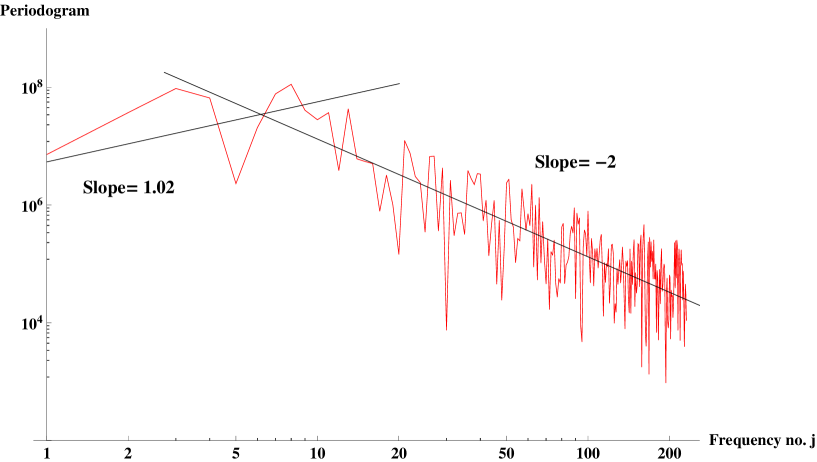
However, as in our case $\eta=-2.02$ (cf. considerations in Sections III.2, III.10 and C.1) the question arises whether the power spectrum, $S_{x}(f)$ , of detrended (time-dependent) signal $x_{t}$ (related to above given unnormalized signal autocorrelation function) properly reproduces the empirical frequency ( $f$ ) dependence of the corresponding periodogram (shown in Figure 29) for small $f$ (i.e., for $1\leq j\leq 14$ ).

By making the Laplace transformation, ${\cal L}(s)$ , of both sides of the third equation in (47) and by using the definition of power spectrum, we obtain for detrended signal

\displaystyle S_{x}(f)\stackrel{{\scriptstyle\rm def.}}{{=}}2Re\,{\cal L}(s)|_{s=2\pi fi}\;\propto\frac{1}{|f|^{\eta+1}}

(48)

where $i$ is an imaginary unit. Notably, this result is well confirmed by plot shown in Figure 29. That is, the slope of the periodogram for small frequencies is directed there by increasing power law with positive slope equals $-(1+\eta)=1.02$ .

By using the fourth equation in (47) and performing an analogous calculation as for $S_{x}(f)$ , we obtain for related power spectrum of the noise

\displaystyle S_{\Delta x}(f)\;\propto\frac{1}{|f|^{\eta-1}},

(49)

which is confirmed by the plot in Figure 31. That is, the slope of the periodogram for small frequencies is directed there by increasing power law with positive slope almost equals $-\eta+1=3.02$ .

Below, we outline the derivation of Expression (48) and hence (49).

Let us assume that function $C(t)\propto(t+t_{0})^{\eta}$ , where $t_{0}$ is a small (insignificant from a physical point of view) positive quantity calculated below. We can derive its Laplace transform in the form GHW ; AE

\displaystyle{\cal L}(s)=\int_{0}^{\infty}C(t)\exp(-st)dt\propto\frac{1}{s^{1+\eta}}\int_{y_{0}}^{\infty}y^{\eta}\exp(-y)dy=\frac{\exp(y_{0})\Gamma_{up}(1+\eta,y_{0})}{s^{1+\eta}},

(50)

where $|y_{0}|=|st_{0}|\ll 1$ and $\Gamma_{up}(1+\eta,y_{o})$ is an upper incomplete gamma function of variable $1+\eta$ . Indeed, Expression (48) was directly obtained from (50) by simply putting there $s=2\pi fi$ and next taking a real part of (50).

The derivation of Expression (49) is analogous to the derivation of Expression (48) if exponent $\eta$ in (50) is formally replaced by exponent $\eta-2$ .

References

(1) D. Sornette, Critical Phenomena in Natural Sciences. Chaos, Fractals, Selforganization and Disorder: Concepts and Tools, Second Eddition, Springer Series in Synergetics, Springer-Verlag, Heidelberg 2004.
(2) A. Schadschneider, D. Chowdhury, K. Nishinari, Stochastic Transport in Complex Systems. From Molecules to Vehicles, Elsevier, Amsterdam 2011.
(3) D. Landau and K. Binder, A Guide to Monte Carlo Simulations in Statistical Physics, Cambridge Univ. Press, Cambridge 2000.
(4) R. Badii, A. Politi, Complexity. Hierarchical structures and scaling in physics, Cambridge Univ. Press, Cambridge 1997.
(5) S. N. Dorogovtsev, A. V. Goltsev, and J. F. F. Mendes, Critical phenomena in complex networks, Rev. Mod. Phys. 80, 1275 (2008).
(6) P. Hohenberg and B. Halperin, Theory of Dynamic Critical Phenomena, Rev. Mod. Phys. 59, 435-479 (1977).
(7) I.A. van de Leemputa, M. Wichersb, A.O.J. Cramerc, D. Borsboomc, F. Tuerlinckxd, P. Kuppensd, E.H. van Nesa, W. Viechtbauerb, E.J. Giltayf, S.H. Aggeng, C. Deromh, N. Jacobsb, K.S. Kendlerg, H.L.J. van der Maasc, M.C. Nealeg, F. Peetersb, E. Thieryl, P. Zacharm, and M. Scheffera: Critical slowing down as early warning for the onset and termination of depression, PNAS, January 7, 2014, 111, No. 1, 87-92.
(8) R. N. Mantegna and H. E. Stanley, An Introduction to Econophysics. Correlations and Complexity in Finance, Cambridge Univ. Press, Cambridge 2000.
(9) B. M. Roehner: Patterns of Speculation. A Study Observational Econophysics, Cambridge Univ. Press, Cambridge 2002.
(10) D. Sornette, Why Stock Markets Crash, Princeton Univ. Press, Princeton and Oxford 2003.
(11) S. Albeverio, V. Jentsch and H. Kantz (Eds.) Extreme Events in Nature and Society, Springer-Verlag, Berlin 2006.
(12) Y. Malevergne and D. Sornette, Extreme Financial Risks. From Dependence to Risk Management, Springer-Verlag, Berlin 2006.
(13) N. F. Johnson, P. Jefferies, P. M. Hui, Financial Market Complexity, Oxford Univ. Press, Oxford 2007.
(14) J. Frey, Exogenous and endogenous market crashes as phase transitions in complex financial systems, EPJ B (2012), in print.
(15) M. Scheffer, J. Bascompte, W. A. Brock, V. Brovkin, S. R. Carpenter, V. Dakos, H. Held, E. H. van Nes, M. Rietkerk, and G. Sugihara, Early-warning signals for critical transitions, Nature 461, 53-59 (2009).
(16) V. Guttal and C. Jayaprakash, Changing skewness: an early warning signal of regime shifts in ecosystems, Ecology Lett., 11, 450-460 (2008).
(17) P. E. McSharry, L. A. Smith, L. Tarassenko, J. Martinerie, M. Le Van Quyen, M. Baulc & B. Ranault, Prediction of epileptic seizures: are nonlinear methods relevant?, Nature Medicine, Lett. Editor 9 (3), 241-242 (2003).
(18) S. R. Carpenter and W. A. Brock, Rising variance: a leading indicator of ecological transitions, Ecology Lett. 9, 308-315 (2006).
(19) S. R. Carpenter, W. A. Brock, J.J. Cole, J.F. Kitchell and M. L. Pace, Leading indicators of trophic cascaders, Ecology Lett. 11, 128-138 (2008).
(20) W. A. Brock, S. R. Carpenter, M. Scheffer, Regime shifts, environmental signals, uncertainty and policy choice in: A Theoretical Framework for Analyzing Social-Ecological Systems, Eds. J. Norberg & G. Cumming, Columbia Univ. Press, New York 2006, pp.
(21) http://en.wikipedia/org/wiki/Econophysics.
(22) D. Sornette: Dragon-Kings, Black Swans and the Prediction of Crises, Int. J. Terraspace and Engineering 2(1), 1-17 (2009).
(23) A. Jakimowicz: Catastrophes and Chaos in Business Cycle Theory, Acta Phys. Pol. A 117(4), 640-646 (2010).
(24) R. Kutner, K. Binder, K.W. Kehr: Diffusion in concentrated lattice gases. V. Particles with repulsive nearest-neighbor interaction on the face-centered-cubic lattice, Phys. Rev. B 28, 1846-1858 (1983).
(25) E. C. Zeeman: Catastrophe Theory: Selected papers, 1972-77, Bull. Amer. Math. Soc. (N. S. ), Volume 84, Number 6, 1360-1368 (1978) & Errata: Bull. Amer. Math. Soc. (N. S. ), Volume 1, Number 4, 681-681 (1979).
(26) J. B. Rosser, Jr.: Implications for Teaching Macroeconomics of Complex Dynamics, Dept. Economics, James Madison Univ., Harrisonburg, 2004.
(27) V. Plerou, P. Gopikrishnan and H. E. Stanley, Two phase behaviour of financial markets, Nature 421(9) 130 (2003).
(28) V. Plerou, P. Gopikrishnan and H. E. Stanley, Two phase behaviour and the distribution of volume, Quantitative Finance 5(6) 519-521 (2005).
(29) M. Potters and J.-P. Bouchaud, Comment on "Two-phase behavior of financial markets", arXiv.cond-mat/0304514v1 23 Apr 2003.
(30) B. Zheng, T. Qiu, and F. Ren, Two-phase phenomena, minority games, and herding, Phys. Rev. E 69 046115/1-6 (2004).
(31) S.M. Jiang, S.M. Cai, T. Shou, and P.L. Zhou, Note on Two-Phase Phenomena in Financial Markets, Chin. Phys. Lett. 25(6) 2319-2322 (2008).
(32) K. Matia, K. Yamasaki, Statistical properties of demand fluctuation in the financial market, Quantitative Finance 5(6) 513-517 (2005).
(33) V. Filimonov and D. Sornette, Spurious trend switching phenomena in financial markets, EPJB (2012), in print.
(34) T. Preis, Econophysics: complex correlations and trend switchings in financial time series, EPJ ST 194(1), 5-86 (2011).
(35) T. Preis, J. J. Schneider, and H. E. Stanley, Switching Phenomena in a System with No Switches, PNAS 108(19, 7674-7678 (2011).
(36) T. Preis and H. E. Stanley, Bubble trouble, Physics World (24), 29-32 (2011).
(37) T. Preis and H. E. Stanley, Switching Phenomena in a System with No Switches, J. Stat. Phys. 138 (1-3), 431-446 (2010).
(38) H. E. Stanley, S. V. Buldyrev, G. Franzese, S. havlin, F. Mallamace, P. Kumar, V. Plerou, and T. Preis, Correlated randomness and switching phenomena, Physica A 389 (15), 2880-2893.
(39) T. Preis and H. E. Stanley, Trend Switching Processes in Financial Markets in Econophysics Approaches to Large-Scale Business Data and Financial Crisis, Eds. M. Takayasu, T. Watanabe, and H. Takayasu, pp. 3-26, Springer-Verlag, Tokyo 2010.
(40) T. Preis and H. E. Stanley, How to Characterize Trend Switching Processes in Financial Markets, Bulletin of the Asia Pacific Center for Theoretical Physics 23, 18-23 (2009).
(41) M. Kozłowska, A. Kasprzak, and R. Kutner: Fractional Market Model and Its Verification on the Warsaw Stock Exchange, Int. J. Modern Phys. C 19(3), 453-469 (2008).
(42) B. Bollobás, Modern Graph Theory, Springer, Berlin 1998.
(43) R. N. Mantegna, Hierarchical structure in financial market, Eur. Phys. J. B 11, 193-197 (1999).
(44) G. Bonanno, G. Calderelli, F. Lillo, S. Micciche, N. Vandewalle, R. N. Mantegna, Networks of equities in financial markets, Eur. Phys. J. B 38, 363-371 (1999).
(45) G. Bonanno, F. Lillo, R. N. Mantegna, High-frequency cross-correlation in a set of stocks, Quant. Fin 1, 96-104 (2001).
(46) N. Vandewalle, F. Brisbois, X. Tordoir, Non-random topology of stock markets, Quant. Fin. 1, 372-374 (2001).
(47) L. Kullmann, J. Kertész, K. Kaski, Time dependent cross correlations between different stock returns: A directed network of influence, Phys. Rev. E 66, 026125 (2002).
(48) M. Tumminello, T. Di. Matteo, T. Aste, and R.N. Mantegna: Correlation based networks of equity returns sampled at different time horizons, EPJ B 55(22), 209-217 (2007).
(49) M. Tumminello, C. Coronello, F. Lillo, S. Micciche, R. N. Mantegna, Spanning Rrees And Bootstrap Reliability Estimation In Correlation-Based Networks, Int. J. Bifurc. and Chaos 17, 2319-2329 (2007).
(50) J. G. Brida, W. A. Risso: Hierarchical structure of the German stock market, Expert Systems with Applications 37, 3846–3852 (2010).
(51) B. M. Tabak, T. R. Serra, D. O. Cajueiro: Topological properties of commodities networks, Eur. Phys. J. B 74, 243–249 (2010).
(52) A. Sienkiewicz, T. Gubiec, R. Kutner, Z. Struzik: Dynamic structural and topological phase transitions on the Warsaw Stock Exchange, Acta Phys. Pol. A 123 (2013), 615-620.
(53) M. Wiliński, A. Sienkiewicz, T. Gubiec, R. Kutner, Z. Struzik: Structural and topological phase transitions on the German Stock Exchange, Physica A 392 (2013), 5963-5973.
(54) M. Wiliński, A. Sienkiewicz, T. Gubiec, R. Kutner, Z. Struzik: Nucleation, condensation and $\lambda$ -transition on a real-life stock market, arXiv:1311.5753 [q-fin.ST].
(55) W. Weidlich, G. Haag: Concepts and Models of a Quantitative Sociology. The Dynamics of Interacting Populations, Springer-Verlag, Berlin 1983.
(56) D. B. West: Introduction to Graph Theory, Prentice–Hall, Englewood Cliffs, New York 1996.
(57) J. B. Kruskal: On the shortest spanning subtree of a graph and the travelling salesman problem, Proc. Am. Math. Soc. 7, 48–50 (1956).
(58) T. R. Werner, T. Gubiec, R. Kutner, D. Sornette: Modeling of super-extreme events: An application to the hierarchical Weierstrass-Mandelbrot Continuous-Time Random Walk, Eur. Phys. J. Special Topics, 2005, 27-52 (2012).
(59) R. Albert, A. -L. Barabási: Statistical Mechanics of Complex Networks, Review of Modern Physics 74, 47-97 (2001).
(60) H. Ebel, L. I. Mielsch, S. Bornholdt: Scale–free topology of e-mail networks, Phys. Rev. E 66 035103–… (2002).
(61) D. J. Watts, S. H. Strogatz: Collective-dynamics of "small–world" networks, Princeton University Press, Princeton, New York 1999.
(62) L. A. N. Amaral, A. Scala, M. Barthelemy, H. E. Stanley: Classes of small-worlds networks, Proceed. of NAS USA 97 (21), 11149-11152 (2000).
(63) M. Faloutsos, P. Faloutsos, Ch. Faloutsos: On power-law relationships of the Internet topology, in SIGCOMM’99, Proceed. of the conf. on applications, technologies, architectures, and protocols for computer communications, 29, 251-262, Harvard University, Science Center, Cambridge, Massachusetts 1999.
(64) Q. Chen, H. Chang, R. Govindan, S. Jamin, S. J. Shenker, W. Willinger: The origin of power laws in Internet topologies revisited, in Proceed. of the $21^{st}$ Annual Joint Conference of the IEEE Computer and Communications Societies 2002, IEEE Computer Society.
(65) A. V. Goltsev, S. N. Dorogovtsev, and J. F. F. Mendes, , Phys. Rev. E 67, 026123–… (2003).
(66) K. Kozłowska and R. Kutner, Singular dynamics of various macroeconomic sectors, Acta Phys. Pol. 117, 630-636 (2010).
(67) R. Kutner, Hierarchical spatio-temporal coupling in fractional wanderings. (I) Continuous-time Weierstrass flights, Physica A 264, 84-106 (1999).
(68) W.A. Fuller, Introduction to statistical time series, J. Wiley & Sons, Inc., Canada 1976.
(69) P. J. Brockwell and R. A. Davis, Time series: Theory and Methods, Springer-Verlag, Berlin 1991.
(70) H. Kantz, Th. Schreiber, Nonlinear time series analysis, Cambridge, Univ. Press, Cambridge 2000.
(71) J. Geweke, S. Porter-Hudak, The Estimation and Application of Long-Memory Time Series Models, J. Time Ser. Anal. 4, 221-237 (1983).
(72) R. Weron, Estimating long-range dependence: finite sample properties and confidence intervals, Physica A 312, 285-299 (2002).
(73) Th. Lux: Network theory is sorely required, Nature Vol. 469, 303-303 (2011).
(74) R. Metzler, J. Klafter, The Random Walk’s Guide to Anomalous Diffusion: A fractional dynamics approach, Phys. Rep. 339, 1-77 (2000).
(75) N. G. van Kampen, Stochastic processes in physics and chemistry, North-Holland, Amsterdam 1987.
(76) C. Wissel, A universal law of the characteristic return time near thresholds, Oecologia (Berlin) 65, 101-107 (1984).
(77) R. Kubo, M. Toda, N. Hascitsume, Statistical Physics II. Nonequilibrium Statistical Mechanics, Springer-Verlag, Berlin 1985.
(78) G. H. Weiss, A Primer of Random Walkology in Frcatals in Science, Eds. A. Bunde amd Sh. Havlin, Springer-Verlag, Berlin 1995.
(79) Tables on Integral Transforms, Vol. I, Based in part, on notes left by H. Bateman and compiled by the staff of the Bateman Manuscript Project, Director A. Erdélyi, McGraw-Hill Book Comp. Inc., New York 1954.

References

[1] D. Sornette, Critical Phenomena in Natural Sciences. Chaos, Fractals, Selforganization and Disorder: Concepts and Tools, Second Eddition, Springer Series in Synergetics, Springer-Verlag, Heidelberg 2004.
[2] A. Schadschneider, D. Chowdhury, K. Nishinari, Stochastic Transport in Complex Systems. From Molecules to Vehicles, Elsevier, Amsterdam 2011.
[3] D. Landau and K. Binder, A Guide to Monte Carlo Simulations in Statistical Physics, Cambridge Univ. Press, Cambridge 2000.
[4] R. Badii, A. Politi, Complexity. Hierarchical structures and scaling in physics, Cambridge Univ. Press, Cambridge 1997.
[5] S. N. Dorogovtsev, A. V. Goltsev, and J. F. F. Mendes, Critical phenomena in complex networks, Rev. Mod. Phys. 80, 1275 (2008).
[6] P. Hohenberg and B. Halperin, Theory of Dynamic Critical Phenomena, Rev. Mod. Phys. 59, 435-479 (1977).
[7] I.A. van de Leemputa, M. Wichersb, A.O.J. Cramerc, D. Borsboomc, F. Tuerlinckxd, P. Kuppensd, E.H. van Nesa, W. Viechtbauerb, E.J. Giltayf, S.H. Aggeng, C. Deromh, N. Jacobsb, K.S. Kendlerg, H.L.J. van der Maasc, M.C. Nealeg, F. Peetersb, E. Thieryl, P. Zacharm, and M. Scheffera: Critical slowing down as early warning for the onset and termination of depression, PNAS, January 7, 2014, 111, No. 1, 87-92.
[8] R. N. Mantegna and H. E. Stanley, An Introduction to Econophysics. Correlations and Complexity in Finance, Cambridge Univ. Press, Cambridge 2000.
[9] B. M. Roehner: Patterns of Speculation. A Study Observational Econophysics, Cambridge Univ. Press, Cambridge 2002.
[10] D. Sornette, Why Stock Markets Crash, Princeton Univ. Press, Princeton and Oxford 2003.
[11] S. Albeverio, V. Jentsch and H. Kantz (Eds.) Extreme Events in Nature and Society, Springer-Verlag, Berlin 2006.
[12] Y. Malevergne and D. Sornette, Extreme Financial Risks. From Dependence to Risk Management, Springer-Verlag, Berlin 2006.
[13] N. F. Johnson, P. Jefferies, P. M. Hui, Financial Market Complexity, Oxford Univ. Press, Oxford 2007.
[14] J. Frey, Exogenous and endogenous market crashes as phase transitions in complex financial systems, EPJ B (2012), in print.
[15] M. Scheffer, J. Bascompte, W. A. Brock, V. Brovkin, S. R. Carpenter, V. Dakos, H. Held, E. H. van Nes, M. Rietkerk, and G. Sugihara, Early-warning signals for critical transitions, Nature 461, 53-59 (2009).
[16] V. Guttal and C. Jayaprakash, Changing skewness: an early warning signal of regime shifts in ecosystems, Ecology Lett., 11, 450-460 (2008).
[17] P. E. McSharry, L. A. Smith, L. Tarassenko, J. Martinerie, M. Le Van Quyen, M. Baulc & B. Ranault, Prediction of epileptic seizures: are nonlinear methods relevant?, Nature Medicine, Lett. Editor 9 (3), 241-242 (2003).
[18] S. R. Carpenter and W. A. Brock, Rising variance: a leading indicator of ecological transitions, Ecology Lett. 9, 308-315 (2006).
[19] S. R. Carpenter, W. A. Brock, J.J. Cole, J.F. Kitchell and M. L. Pace, Leading indicators of trophic cascaders, Ecology Lett. 11, 128-138 (2008).
[20] W. A. Brock, S. R. Carpenter, M. Scheffer, Regime shifts, environmental signals, uncertainty and policy choice in: A Theoretical Framework for Analyzing Social-Ecological Systems, Eds. J. Norberg & G. Cumming, Columbia Univ. Press, New York 2006, pp.
[21] http://en.wikipedia/org/wiki/Econophysics.
[22] D. Sornette: Dragon-Kings, Black Swans and the Prediction of Crises, Int. J. Terraspace and Engineering 2(1), 1-17 (2009).
[23] A. Jakimowicz: Catastrophes and Chaos in Business Cycle Theory, Acta Phys. Pol. A 117(4), 640-646 (2010).
[24] R. Kutner, K. Binder, K.W. Kehr: Diffusion in concentrated lattice gases. V. Particles with repulsive nearest-neighbor interaction on the face-centered-cubic lattice, Phys. Rev. B 28, 1846-1858 (1983).
[25] E. C. Zeeman: Catastrophe Theory: Selected papers, 1972-77, Bull. Amer. Math. Soc. (N. S. ), Volume 84, Number 6, 1360-1368 (1978) & Errata: Bull. Amer. Math. Soc. (N. S. ), Volume 1, Number 4, 681-681 (1979).
[26] J. B. Rosser, Jr.: Implications for Teaching Macroeconomics of Complex Dynamics, Dept. Economics, James Madison Univ., Harrisonburg, 2004.
[27] V. Plerou, P. Gopikrishnan and H. E. Stanley, Two phase behaviour of financial markets, Nature 421(9) 130 (2003).
[28] V. Plerou, P. Gopikrishnan and H. E. Stanley, Two phase behaviour and the distribution of volume, Quantitative Finance 5(6) 519-521 (2005).
[29] M. Potters and J.-P. Bouchaud, Comment on "Two-phase behavior of financial markets", arXiv.cond-mat/0304514v1 23 Apr 2003.
[30] B. Zheng, T. Qiu, and F. Ren, Two-phase phenomena, minority games, and herding, Phys. Rev. E 69 046115/1-6 (2004).
[31] S.M. Jiang, S.M. Cai, T. Shou, and P.L. Zhou, Note on Two-Phase Phenomena in Financial Markets, Chin. Phys. Lett. 25(6) 2319-2322 (2008).
[32] K. Matia, K. Yamasaki, Statistical properties of demand fluctuation in the financial market, Quantitative Finance 5(6) 513-517 (2005).
[33] V. Filimonov and D. Sornette, Spurious trend switching phenomena in financial markets, EPJB (2012), in print.
[34] T. Preis, Econophysics: complex correlations and trend switchings in financial time series, EPJ ST 194(1), 5-86 (2011).
[35] T. Preis, J. J. Schneider, and H. E. Stanley, Switching Phenomena in a System with No Switches, PNAS 108(19, 7674-7678 (2011).
[36] T. Preis and H. E. Stanley, Bubble trouble, Physics World (24), 29-32 (2011).
[37] T. Preis and H. E. Stanley, Switching Phenomena in a System with No Switches, J. Stat. Phys. 138 (1-3), 431-446 (2010).
[38] H. E. Stanley, S. V. Buldyrev, G. Franzese, S. havlin, F. Mallamace, P. Kumar, V. Plerou, and T. Preis, Correlated randomness and switching phenomena, Physica A 389 (15), 2880-2893.
[39] T. Preis and H. E. Stanley, Trend Switching Processes in Financial Markets in Econophysics Approaches to Large-Scale Business Data and Financial Crisis, Eds. M. Takayasu, T. Watanabe, and H. Takayasu, pp. 3-26, Springer-Verlag, Tokyo 2010.
[40] T. Preis and H. E. Stanley, How to Characterize Trend Switching Processes in Financial Markets, Bulletin of the Asia Pacific Center for Theoretical Physics 23, 18-23 (2009).
[41] M. Kozłowska, A. Kasprzak, and R. Kutner: Fractional Market Model and Its Verification on the Warsaw Stock Exchange, Int. J. Modern Phys. C 19(3), 453-469 (2008).
[42] B. Bollobás, Modern Graph Theory, Springer, Berlin 1998.
[43] R. N. Mantegna, Hierarchical structure in financial market, Eur. Phys. J. B 11, 193-197 (1999).
[44] G. Bonanno, G. Calderelli, F. Lillo, S. Micciche, N. Vandewalle, R. N. Mantegna, Networks of equities in financial markets, Eur. Phys. J. B 38, 363-371 (1999).
[45] G. Bonanno, F. Lillo, R. N. Mantegna, High-frequency cross-correlation in a set of stocks, Quant. Fin 1, 96-104 (2001).
[46] N. Vandewalle, F. Brisbois, X. Tordoir, Non-random topology of stock markets, Quant. Fin. 1, 372-374 (2001).
[47] L. Kullmann, J. Kertész, K. Kaski, Time dependent cross correlations between different stock returns: A directed network of influence, Phys. Rev. E 66, 026125 (2002).
[48] M. Tumminello, T. Di. Matteo, T. Aste, and R.N. Mantegna: Correlation based networks of equity returns sampled at different time horizons, EPJ B 55(22), 209-217 (2007).
[49] M. Tumminello, C. Coronello, F. Lillo, S. Micciche, R. N. Mantegna, Spanning Rrees And Bootstrap Reliability Estimation In Correlation-Based Networks, Int. J. Bifurc. and Chaos 17, 2319-2329 (2007).
[50] J. G. Brida, W. A. Risso: Hierarchical structure of the German stock market, Expert Systems with Applications 37, 3846–3852 (2010).
[51] B. M. Tabak, T. R. Serra, D. O. Cajueiro: Topological properties of commodities networks, Eur. Phys. J. B 74, 243–249 (2010).
[52] A. Sienkiewicz, T. Gubiec, R. Kutner, Z. Struzik: Dynamic structural and topological phase transitions on the Warsaw Stock Exchange, Acta Phys. Pol. A 123 (2013), 615-620.
[53] M. Wiliński, A. Sienkiewicz, T. Gubiec, R. Kutner, Z. Struzik: Structural and topological phase transitions on the German Stock Exchange, Physica A 392 (2013), 5963-5973.
[54] M. Wiliński, A. Sienkiewicz, T. Gubiec, R. Kutner, Z. Struzik: Nucleation, condensation and $\lambda$ -transition on a real-life stock market, arXiv:1311.5753 [q-fin.ST].
[55] W. Weidlich, G. Haag: Concepts and Models of a Quantitative Sociology. The Dynamics of Interacting Populations, Springer-Verlag, Berlin 1983.
[56] D. B. West: Introduction to Graph Theory, Prentice–Hall, Englewood Cliffs, New York 1996.
[57] J. B. Kruskal: On the shortest spanning subtree of a graph and the travelling salesman problem, Proc. Am. Math. Soc. 7, 48–50 (1956).
[58] T. R. Werner, T. Gubiec, R. Kutner, D. Sornette: Modeling of super-extreme events: An application to the hierarchical Weierstrass-Mandelbrot Continuous-Time Random Walk, Eur. Phys. J. Special Topics, 2005, 27-52 (2012).
[59] R. Albert, A. -L. Barabási: Statistical Mechanics of Complex Networks, Review of Modern Physics 74, 47-97 (2001).
[60] H. Ebel, L. I. Mielsch, S. Bornholdt: Scale–free topology of e-mail networks, Phys. Rev. E 66 035103–… (2002).
[61] D. J. Watts, S. H. Strogatz: Collective-dynamics of "small–world" networks, Princeton University Press, Princeton, New York 1999.
[62] L. A. N. Amaral, A. Scala, M. Barthelemy, H. E. Stanley: Classes of small-worlds networks, Proceed. of NAS USA 97 (21), 11149-11152 (2000).
[63] M. Faloutsos, P. Faloutsos, Ch. Faloutsos: On power-law relationships of the Internet topology, in SIGCOMM’99, Proceed. of the conf. on applications, technologies, architectures, and protocols for computer communications, 29, 251-262, Harvard University, Science Center, Cambridge, Massachusetts 1999.
[64] Q. Chen, H. Chang, R. Govindan, S. Jamin, S. J. Shenker, W. Willinger: The origin of power laws in Internet topologies revisited, in Proceed. of the $21^{st}$ Annual Joint Conference of the IEEE Computer and Communications Societies 2002, IEEE Computer Society.
[65] A. V. Goltsev, S. N. Dorogovtsev, and J. F. F. Mendes, , Phys. Rev. E 67, 026123–… (2003).
[66] K. Kozłowska and R. Kutner, Singular dynamics of various macroeconomic sectors, Acta Phys. Pol. 117, 630-636 (2010).
[67] R. Kutner, Hierarchical spatio-temporal coupling in fractional wanderings. (I) Continuous-time Weierstrass flights, Physica A 264, 84-106 (1999).
[68] W.A. Fuller, Introduction to statistical time series, J. Wiley & Sons, Inc., Canada 1976.
[69] P. J. Brockwell and R. A. Davis, Time series: Theory and Methods, Springer-Verlag, Berlin 1991.
[70] H. Kantz, Th. Schreiber, Nonlinear time series analysis, Cambridge, Univ. Press, Cambridge 2000.
[71] J. Geweke, S. Porter-Hudak, The Estimation and Application of Long-Memory Time Series Models, J. Time Ser. Anal. 4, 221-237 (1983).
[72] R. Weron, Estimating long-range dependence: finite sample properties and confidence intervals, Physica A 312, 285-299 (2002).
[73] Th. Lux: Network theory is sorely required, Nature Vol. 469, 303-303 (2011).
[74] R. Metzler, J. Klafter, The Random Walk’s Guide to Anomalous Diffusion: A fractional dynamics approach, Phys. Rep. 339, 1-77 (2000).
[75] N. G. van Kampen, Stochastic processes in physics and chemistry, North-Holland, Amsterdam 1987.
[76] C. Wissel, A universal law of the characteristic return time near thresholds, Oecologia (Berlin) 65, 101-107 (1984).
[77] R. Kubo, M. Toda, N. Hascitsume, Statistical Physics II. Nonequilibrium Statistical Mechanics, Springer-Verlag, Berlin 1985.
[78] G. H. Weiss, A Primer of Random Walkology in Frcatals in Science, Eds. A. Bunde amd Sh. Havlin, Springer-Verlag, Berlin 1995.
[79] Tables on Integral Transforms, Vol. I, Based in part, on notes left by H. Bateman and compiled by the staff of the Bateman Manuscript Project, Director A. Erdélyi, McGraw-Hill Book Comp. Inc., New York 1954.

	$\displaystyle\frac{a_{1}}{a_{0}}=-(x_{1^{\prime\prime}}^{}+x_{1^{\prime}}^{}+x_{1}^{*}),$
	$\displaystyle\frac{a_{2}}{a_{0}}=x_{1^{\prime}}^{}x_{1^{\prime\prime}}^{}+x_{1}^{}x_{1^{\prime\prime}}^{}+x_{1}^{}x_{1^{\prime}}^{},$
	$\displaystyle\frac{a_{3}}{a_{0}}=-x_{1}^{}\,x_{1^{\prime}}^{}\,x_{1^{\prime\prime}}^{*}.$		(37)

Empirical symptoms of catastrophic bifurcation transitions on financial markets: A phenomenological approach

Abstract

pacs:

I Introduction

II Structural phase transitions on financial markets

II.1 Initial results and discussion

II.2 Initial conclusions

III Systematic analysis of empirical data

III.1 Signals and detrended signals

III.2 Noise and its distributions

III.3 Usual variance of detrended signal

III.4 Accumulative variance of detrended signal

III.5 Recovery rate

III.6 Empirical catastrophic bifurcation transitions

III.7 Nonlinear indicator: skewness

III.8 Periodograms

III.9 Periodograms of signals

III.10 Periodograms of noises

IV Qualitative explanation

V Conclusions

Acknowledgements.

Appendix A Detrending procedure

Appendix B Linear indicators of a critical slowing down from bifurcation point of view

B.0.1 Continuous-time formulation

B.1 Analysis of the linear stability

B.2 Generic properties of the first order autoregressive time series

B.3 Nonlinear time series analysis

B.4 Catastrophic dynamics next to catastrophic bifurcation transition

B.5 Simplest example: approximation of force f𝑓f by the third-order polynomial

B.5.1 Case of the catastrophic bifurcation transition

B.5.2 Case before the catastrophic bifurcation transition

B.5.3 Case after the catastrophic bifurcation transition

Appendix C Scaling relations

C.1 Autocorrelation and power spectrum

References

References

Empirical symptoms of catastrophic bifurcation transitions
on financial markets: A phenomenological approach

B.5 Simplest example: approximation of force $f$ by the third-order polynomial