1 Introduction

Scalar field models have played a vital role in cosmological theoretical studies in nearly half a century. Those assumed scalar fields appeared in different cosmological research aspects to settle different cosmological problems [1], such as to drive inflation, to explain a time variable cosmological ^′constant^′ and so on. After the discovery of the accelerating expansion of universe, scalar fields have played another important essential role as a candidate of dark energy . There are so many phenomenological dark energy models of scalar fields, such as quintessence, phantom, quintom and the scalar fields with non-canonical kinetic energy term (for a review, see[2, 3]).

Phase-plane analysis is a very useful and common method(see Ref[21] and recent papers, e.g. [5, 6, 7, 8]) to study the dynamical evolution of those scalar fields models and their cosmological implications. However, most of those works only focus on the quintessence models(including phantom quintessence and quintom) with unique exponential potential and tachyon models(including phantom tachyon) with inverse square potential, and correspondingly, the dynamical systems are two dimensional autonomous system(see the references cited in [11, 27]). Using a method which considers the potential related variable $\Gamma$ as a function of another potential related variable $\lambda$ (see Eq.(10) for the definition of $\Gamma$ and $\lambda$)[46, 11, 27], we are able to analyze the phase-plane of the dynamical systems of the quintessence and tachyon models with many different potentials. When the potentials are beyond the special type such as exponential or inverse square potentials, the dynamical systems consequently become a three-dimensional autonomous systems. This method is quite effective and powerful, it therefore has been generalized to several other cosmological contexts[12, 13, 14, 15, 16, 17, 18, 19, 45, 20]. However, there is very few work focusing on the dynamical behavior of the scalar field with a general modified kinetic term, such as k-essence ($L=V(\phi)F(X)$) and general non-canonical scalar field ($L=F(X)-V(\phi)$). Recently, Josue De-Santiago et. al analyzed the dynamical system of general non-canonical scalar field with the lagrangian $L=F(X)-V(\phi)$ and studied the phase plane after a suitable choice of variables[40]. They obtained the three-dimensional autonomous system of this non-canonical scalar field after specifying the kinetic term as $F(X)=AX^{\eta}$ and choosing the potential as $V(\phi)=V_{0}(\phi-\phi_{0})^{1/(1-\Gamma)}$(i.e., a special case that $\Gamma=const$) and studied the critical points as well as their stability.

Motivated by the work[40], we try to extend our works[11, 27] in this paper to give the three-dimensional autonomous dynamical systems for most of the popular scalar field dark energy models including (phantom) quintessence, (phantom) tachyon, k-essence and general non-canonical scalar field models in current work. We will show that the three-dimensional autonomous systems of general non-canonical scalar field and k-essence will reduce to the quintessence and tachyon scalar field respectively. Not like most of the previous works, here we express the three dimensional autonomous systems from variables $(x,y,\lambda)$ to the observable related variables $(w_{\phi},\Omega_{\phi},\lambda)$. It will be very convenient to investigate the dynamical properties of the autonomous system based on the observable related variables $w_{\phi}$ and $\Omega_{\phi}$(see [21, 22, 23, 24, 25, 26, 27, 28] and a recent paper about the general property of dynamical quintessence field[30]). Since the definition of the variables $x$ and $y$ could vary with different scalar field models, while the meaning of $w_{\phi}$ and $\Omega_{\phi}$ are the same for different dark energy models and therefore the differential equations of $w_{\phi}$ and $\Omega_{\phi}$ are model independent. The paper is organized as follows. We firstly present the basic theoretical framework for (phantom) quintessence, (phantom) tachyon, k-essence and general non-canonical scalar field models in section 2, and try to give the relationships between those different scalar fields in this section. We then give the three dimensional autonomous dynamical systems for those scalar fields and switch the dynamical variables from $(x,y)$ to $(w_{\phi},\Omega_{\phi})$ in each subsection of section 3. Additionally, using the dynamical systems, we give the exact solution of $w_{\phi}$ and $\Omega_{\phi}$ for a special case of tachyon model when the potential is chosen to be a constant in subsection 3.2. We show that the dynamical autonomous system of k-essence can reduce to tachyon model, and investigate another special case called kinetically driven quintessence with the lagrangian $p(X,\phi)=f(\phi)(-X+X^{2})$ detailedly in subsection 3.3. In subsection 3.4, we show that the dynamical autonomous system of general non-canonical scalar field can reduce to quintessence and tachyon model respectively for some special cases. We also studied two special cases of purely kinetic united model $L=F(X)$ in detailed in this subsection. We try to give the cosmological implications of the three-dimensional dynamical autonomous system and present the conclusion in section 4. We also raise a question about the possibility of the chaotic behavior in the spatially flat single scalar field FRW cosmological models in the presence of the ordinary matter.

2 Basic Framework for various Scalar Fields

Let us restrict ourselves to a flat universe described by the FRW metric, and consider a spatially homogeneous real scalar field $\phi$ with non-canonical kinetic energy term. The lagrangian density is given as

$$L=L(X,V)$$ (1)

where $L$ is a function of $X$ and potential $V(\phi)$, $X=\frac{1}{2}\nabla_{\mu}\phi\nabla^{\mu}\phi=\frac{1}{2}{\dot{\phi}}^{2}$ for a spatially homogeneous scalar field. The pressure, energy density and the Friedmann equations of the scalar field could be easily obtained as following:

$$p_{\phi}=L(X,V)$$ (2)

$$\rho_{\phi}=2XL_{X}-L$$ (3)

$$H^{2}=(\frac{\dot{a}}{a})^{2}=\frac{1}{3M^{2}_{pl}}[\rho_{\phi}+\rho_{b}]$$ (4)

$$\dot{H}=-\frac{1}{2M^{2}_{pl}}[2XL_{X}+\gamma_{b}\rho_{b}]$$ (5)

where $8\pi G=\kappa^{2}=1/M^{2}_{pl}$, $\rho_{b}$ is the density of a barotropic fluid component with the equation of state $p_{b}=w_{b}\rho_{b}=(\gamma_{b}-1)\rho_{b}$. $\gamma_{b}=1$ for matter and $\gamma_{b}=4/3$ for radiation. $L_{X}$ is the derivative of $L(X,\phi)$ with respect to $X$.

For quintessence, general non-canonical scalar field, tachyon and K-essence model, the pressure $p$ and energy density $\rho$ are respectively:

$$p_{q}=\varsigma\frac{1}{2}\dot{\phi}^{2}-V(\phi),\rho_{q}=\varsigma\frac{1}{2}\dot{\phi}^{2}+V(\phi)$$ (6)

$$p_{g}=F(X)-V(\phi),\rho_{g}=2XF_{X}-F(X)+V(\phi)$$ (7)

$$p_{t}=-V(\phi)\sqrt{1-\varsigma\dot{\phi}^{2}},\rho_{t}=\frac{V(\phi)}{\sqrt{1-\varsigma\dot{\phi}^{2}}}$$ (8)

$$p_{K}=-V(\phi)F(X),\rho_{K}=2L_{X}X-L(X,\phi)=V(\phi)(F-2XF_{X})$$ (9)

If $\varsigma=1$, Eq.(6) and Eq.(8) correspond to the quintessence and tachyon scalar field. If $\varsigma=-1$, Eq.(6) and Eq.(8) correspond to the phantom quintessence and phantom tachyon scalar field. General non-canonical scalar field Eq.(7) can recover to (phantom) quintessence Eq.(6) if $F(X)=\varsigma{\dot{\phi}}^{2}=2\varsigma X$. K-essence model Eq.(9) can recover to (phantom) tachyon Eq.(8) if $F(X)=\sqrt{1-\varsigma\dot{\phi}^{2}}=\sqrt{1-2\varsigma X}$. Moreover, if the scalar field is redefined, it is demonstrated that K-essence model described by Eq.(9) with a linear kinetic function $F(X)=X+1$ can reduce to any quintessence model described by Eq.(6). It means that any quintessence can be contained into K-essence frame, so each quintessence model is kinematically equivalent to a k-essence model. The authors also give the relationship between the potentials of the two models[9]. For example, the exponential potential $V(\phi)=V_{0}e^{-\lambda\phi}$ in quintessence model plays the similar role as the inverse square potential $V(\phi)=(\frac{1}{2}\kappa\lambda\phi-c_{1})^{-2}$. We will also show that the role of inverse square potential in k-essence model is very similar with exponential potential in quintessence in the next section.

3 Dynamical System of various Scalar Fields

In this section, we will give the dynamical system for all the quintessence, tachyon, K-essence and general non-canonical scalar field model. We will summarize the dynamical system analysis and give our comments.

3.1 Dynamical System for Quintessence and Phantom Quintessence Scalar Field

For the (phantom) quintessence scalar field with lagrangian $L=\varsigma\frac{1}{2}\dot{\phi}^{2}-V(\phi)$, we can define the following dimensionless variables:

$$x=\frac{\kappa\dot{\phi}}{\sqrt{6}H},y=\frac{\kappa\sqrt{V}}{\sqrt{3}H},~{}\lambda(\phi)=-\frac{V^{\prime}}{V},\Gamma(\phi)=\frac{VV^{\prime\prime}}{V^{\prime 2}}$$ (10)

Where $V^{\prime}=dV(\phi)/d\phi,V^{\prime\prime}=d^{2}V(\phi)/d\phi^{2}$. The parameters $\Gamma(\phi)$ and $\lambda(\phi)$ of the potentials can be related with the famous slow roll parameters $\epsilon_{V}$ and $\eta_{V}$(e.g., see [10]):

$$\epsilon_{V}(\phi)=\frac{M^{2}_{pl}}{2}(\frac{V^{\prime}}{V})^{2}=\frac{M^{2}_{pl}}{2}\lambda^{2}(\phi)$$ (11)

$$\eta_{V}(\phi)=M^{2}_{pl}\frac{V^{\prime\prime}}{V}=M^{2}_{pl}\frac{V}{V^{\prime 2}}\frac{V^{\prime\prime}}{V}\frac{V^{\prime 2}}{V}=M^{2}_{pl}\Gamma(\phi)\lambda^{2}(\phi)$$ (12)

Using Eq.(4), Eq.(5),Eq.(6)and Eq.(7), We can write down the following equations for the evolution of the (phantom) quintessence:

$$\frac{dx}{dN}=-3x+\frac{\sqrt{6}}{2}\varsigma\lambda y^{2}+\frac{3}{2}x[\varsigma(1-w_{b})x^{2}+(1+w_{b})(1-y^{2})]$$ (13)

$$\frac{dy}{dN}=-\frac{\sqrt{6}}{2}\lambda xy+\frac{3}{2}y[\varsigma(1-w_{b})x^{2}+(1+w_{b})(1-y^{2})]$$ (14)

$$\frac{d\lambda}{dN}=-\sqrt{6}\lambda^{2}(\Gamma-1)x$$ (15)

where $N=ln(a)$, $a$ is the scale factor. $\varsigma=1$ or $-1$ for quintessence and phantom quintessence model. Here we should emphasize that Eqs.(13-15) is not a dynamical autonomous system since the parameter $\Gamma(\phi)$ is unknown. The energy density fraction of dark energy scalar field is

$$\Omega_{\phi}=\frac{\rho_{\phi}}{3M^{2}_{pl}H^{2}}=\varsigma x^{2}+y^{2}$$ (16)

while the equation of state of the dark energy scalar field is

$$\gamma_{\phi}=1+w_{\phi}=1+\frac{\varsigma x^{2}-y^{2}}{\varsigma x^{2}+y^{2}}=\frac{2\varsigma x^{2}}{\varsigma x^{2}+y^{2}}=\frac{2\varsigma x^{2}}{\Omega_{\phi}}$$ (17)

In the other hand, it is more convenient to rewrite the dynamical system Eqs.(13-14) from the dependent variables $(x,y,\lambda)$ directly to the observable quantities $(\Omega_{\phi},\gamma_{\phi},\lambda)$[24]:

$$\frac{d\Omega_{\phi}}{dN}=3(\gamma_{b}-\gamma_{\phi})\Omega_{\phi}(1-\Omega_{\phi})$$ (18)

$$\frac{d\gamma_{\phi}}{dN}=(2-\gamma_{\phi})(\lambda\sqrt{3\varsigma\gamma_{\phi}\Omega_{\phi}}-3\gamma_{\phi})$$ (19)

$$\frac{d\lambda}{dN}=-\sqrt{3}\lambda^{2}(\Gamma-1)\sqrt{\varsigma\gamma_{\phi}\Omega_{\phi}}$$ (20)

Eqs.(18-20) can reduce to quintessence when $\varsigma=1$ (Eqs(3-5) in paper [25] or Eqs.(17-18) in paper [24]) and reduce to phantom quintessence when $\varsigma=-1$ [23]. Eqs.(18-20) are very useful to study the cosmological implication of the evolutional behavior of the dynamical system because the dynamical variables $\Omega_{\phi}$ and $\gamma_{\phi}$ are the observable quantities. For example, $d\gamma_{\phi}/dN>0$ corresponds to the thawing model and $d\gamma_{\phi}/dN<0$ corresponds to the freezing model of the evolution of equation of state of dark energy [26, 25].

If $\Gamma=1$, Eq.(15)(or Eqs.(20)) will disappear, Eqs.(13-14)(or Eqs.(18-19)) will become a two-dimensional dynamical autonomous system. $\Gamma=1$ corresponds to the exponential potential $V_{0}e^{-\lambda\phi}$, which has been studied in many literatures(e.g., see the references of paper [11]). However, the system described by Eqs.(13-15)(or Eqs.(18-20)) are not a dynamical autonomous system for other potentials because the potential related parameter $\Gamma$ is unknown. Since $\lambda$ is a function of quintessence scalar field $\phi$ and $\Gamma$ is also a function of $\phi$, then $\Gamma$ can generally be expressed as a function of $\lambda$. So if we consider $\Gamma$ as a function of $\lambda$, namely $\Gamma=\Gamma(\lambda)$, then Eqs.(13-15)(or Eqs.(18-20)) are definitely a dynamical autonomous system, we therefore can study its properties and dynamical evolution using the phase plane and critical points analysis. Moreover, considering $\Gamma$ as a function of $\lambda$ can cover many potentials beyond the exponential potential[11].

3.2 Dynamical System for tachyon and Phantom tachyon Scalar Field

For the tachyon and phantom tachyon scalar field with lagrangian $L=-V(\phi)\sqrt{1-\varsigma\dot{\phi}^{2}}$, we can define the dimensionless variables as follows:

$$x=\dot{\phi},y=\frac{\kappa\sqrt{V}}{\sqrt{3}H},\lambda=\frac{V^{\prime}}{\kappa V^{3/2}},\Gamma=\frac{VV^{\prime\prime}}{V^{\prime 2}}$$ (21)

Where $V^{\prime}=dV(\phi)/d\phi,V^{\prime\prime}=d^{2}V(\phi)/d\phi^{2}$. Using Eq.(4), Eq.(5),Eq.(6)and Eq.(21), the evolution of (phantom) tachyon can be discribed in the following dynamical form [27]:

$$\frac{dx}{dN}=-\sqrt{3}(1-\varsigma x^{2})(\sqrt{3}x+\varsigma\lambda y)$$ (22)

$$\frac{dy}{dN}=\frac{\sqrt{3}}{2}y(\lambda xy+\frac{\sqrt{3}y^{2}(\varsigma x^{2}-\gamma_{b})}{\sqrt{1-\varsigma x^{2}}}+\sqrt{3}\gamma_{b})$$ (23)

$$\frac{d\lambda}{dN}=\sqrt{3}xy\lambda^{2}(\Gamma-\frac{3}{2})$$ (24)

The density parameter of tachyon field $\Omega_{\phi}$, the equation of state $w_{\phi}$ are:

$$\Omega_{\phi}=\frac{y^{2}}{\sqrt{1-\varsigma x^{2}}}$$ (25)

$$\gamma_{\phi}=1+w_{\phi}=\varsigma x^{2}$$ (26)

We can also rewrite the the dynamical system Eqs.(22-24) from the dependent variables $(x,y,\lambda)$ directly to the observable quantities $(\Omega_{\phi},\gamma_{\phi},\lambda)$:

$$\frac{d\Omega_{\phi}}{dN}=3(\gamma_{b}-\gamma_{\phi})\Omega_{\phi}(1-\Omega_{\phi})$$ (27)

$$\frac{d\gamma_{\phi}}{dN}=-2(1-\gamma_{\phi})[3\gamma_{\phi}+\lambda\sqrt{3\varsigma\gamma_{\phi}\Omega_{\phi}}(1-\gamma_{\phi})^{\frac{1}{4}}]$$ (28)

$$\frac{d\lambda}{dN}=\sqrt{3\varsigma\gamma_{\phi}\Omega_{\phi}}(1-\gamma_{\phi})^{\frac{1}{4}}\lambda^{2}(\Gamma-\frac{3}{2})$$ (29)

The above equations Eqs.(27-29) are also obtained in [28, 29]. The critical points and the dynamical evolution of this system describing by Eqs.(22-24) or Eqs.(27-29) had been studied in [27].

If $\Gamma=3/2$, Eq.(24)(or Eqs.(29)) will disappear, Eqs.(22-23)(or Eqs.(27-28)) will become a two-dimensional dynamical autonomous system. For (phantom) tachyon scalar field, $\Gamma=3/2$ corresponds to the case that the form of potential is inverse square potential. But for other potentials, the system described by Eqs.(22-24)(or Eqs.(27-29)) will not be a dynamical autonomous system any more since the potential related parameter $\Gamma$ is unknown, and we can not exactly analyze the evolution of universe like the inverse square potential any more. However, since $\lambda$ is the function of tachyon field $\phi$ and $\Gamma$ is also the function of $\phi$, $\Gamma$ can be generally expressed as a function of $\lambda$. So as the method used in[11], we can consider $\Gamma$ as a function of $\lambda$, $\Gamma=\Gamma(\lambda)$, then Eqs.(22-24)(or Eqs.(27-29)) will become a dynamical autonomous system, we therefore can study its properties and dynamical evolution using the phase plane and critical points analysis. For each form of function $\Gamma(\lambda)$, we can figure out the detailed form of potential, so this method can cover many potentials beyond the inverse square potential[27].

For the most simple case of potential $V(\phi)=V_{0}$, $\lambda=0$, Eqs.(27-29) become a very simple differential equation:

$$\frac{d\Omega_{\phi}}{dN}=3(\gamma_{b}-\gamma_{\phi})\Omega_{\phi}(1-\Omega_{\phi}),~{}\frac{d\gamma_{\phi}}{dN}=-6\gamma_{\phi}(1-\gamma_{\phi})$$ (30)

We can get the exact solution for the above equations:

$$\gamma_{\phi}=\frac{1}{1+c_{1}e^{6N}},~{}\Omega_{\phi}=\frac{\sqrt{1+c_{1}e^{6N}}}{\sqrt{1+c_{1}e^{6N}}+c_{2}(e^{6N})^{(1-\gamma_{b})/2}}$$ (31)

Tachyon scalar field with this constant potential had been studied in[34]. According to the best-fit values of the parameters they obtained, we can obtain the value of the integral constant $c_{1}=0.0082$ and $c_{2}=0.59$ here. We know from Eq.(31), when $N\rightarrow+\infty$, we have $\gamma_{\phi}\rightarrow 0$ and $\Omega_{\phi}\rightarrow 1$, the universe will be a de Sitter like universe filled with the tachyon scalar field.

3.3 Dynamical System for K-essence Scalar Field

For the k-essence scalar field with lagrangian $L=-V(\phi)F(X)$, we define the following dimensionless variables as the same as Eq.(21):

$$x=\dot{\phi},\ \ y=\frac{\kappa\sqrt{V}}{\sqrt{3}H},\ \lambda=\frac{V^{\prime}}{\kappa V^{3/2}},\ \Gamma=\frac{VV^{\prime\prime}}{V^{\prime 2}}$$ (32)

Using Eq.(4), Eq.(5),Eq.(6)and Eq.(32), we can get following dynamical system:

$$\frac{dx}{dN}=\frac{-\sqrt{3}}{F_{X}+2XF_{XX}}[\sqrt{3}xF_{X}-y\lambda(F-2XF_{X})]$$ (33)

$$\frac{dy}{dN}=\frac{y}{2}[\sqrt{3}\lambda xy+6XF_{X}(\gamma_{b}-1)y^{2}-3\gamma_{b}Fy^{2}+3\gamma_{b}]$$ (34)

$$\frac{d\lambda}{dN}=\sqrt{3}xy\lambda^{2}(\Gamma-\frac{3}{2})$$ (35)

The density parameter of tachyon scalar field $\Omega_{\phi}$, the equation of state $w_{\phi}$ are:

$$\Omega_{\phi}=(F-2XF_{X})y^{2}=(F-xF^{\prime})y^{2}$$ (36)

$$\gamma_{\phi}=\frac{xF^{\prime}}{xF^{\prime}-F}=-\frac{xy^{2}F^{\prime}}{\Omega_{\phi}}$$ (37)

Where $F^{\prime}=dF(X)/dx$ and $F^{\prime\prime}=d^{2}F(X)/dx^{2}$, they both are the functions of $x$. Using Eq.(36) and Eq.(37), we can also rewrite the dynamical system Eq.(33), Eq.(34) and Eq.(35) from the dependent variables $(x,y,\lambda)$ directly to the observable quantities $(\Omega_{\phi},\gamma_{\phi},\lambda)$:

$$\frac{d\Omega_{\phi}}{dN}=3(\gamma_{b}-\gamma_{\phi})\Omega_{\phi}(1-\Omega_{\phi})$$ (38)

$$\frac{d\gamma_{\phi}}{dN}=-\frac{\sqrt{3}(\lambda xy+\sqrt{3}\gamma_{\phi})[xF^{\prime\prime}(1-\gamma_{\phi})+F^{\prime}]}{xF^{\prime\prime}}=\sqrt{3}(\lambda xy+\sqrt{3}\gamma_{\phi})(\gamma_{\phi}-1-\frac{1}{2\Xi+1})$$ (39)

$$\frac{d\lambda}{dN}=\sqrt{3}xy\lambda^{2}(\Gamma-\frac{3}{2})$$ (40)

where $\Xi=XF_{XX}/F_{X}=(xF^{\prime\prime}-F^{\prime})/2F^{\prime}$. We have pointed out the relationship between quintessence and K-essence in previous section. k-essence model described by Eq.(9) with a linear kinetic function $F(X)=X+1$ can reduce to any quintessence model described by Eq.(6)[9]. So all quintessence model with any potentials can be considered as the special cases of k-essence model. Moreover, it proved that the correspondence of the exponential potential $V(\phi)=V_{0}e^{-\lambda\phi}$ in quintessence model is exactly the inverse square potential $V(\phi)=(\frac{1}{2}\kappa\lambda\phi-c_{1})^{-2}$ in k-essence model. This can explain why the dynamical system Eqs.(13-15)(or Eqs.(18-20)) of quintessence reduces to two-dimensional autonomous system for exponential potential($\Gamma=1$) while the same situation happens for inverse square potential ($\Gamma=3/2$) in tachyon and k-essence model. Author had considered another non-canonical scalar field lagrangian defined as $L_{\phi}=Vf(B)$ with $B=X/V$[35]. It also includes the canonical quintessence if we chose $f(B)=B-1$.

Let us discuss whether Eqs.(38-40) could be considered as an autonomous system. Firstly, we realized that the variables $x$ and $y$ still appear in Eq.(39) because we do not know the detailed form of function $F(X)$ and can not figure out the solution of $x$ and $y$. However, from Eqs.(36-37), we are sure that variables $x$ and $y$ are the functions of variables $\Omega_{\phi}$ and $\gamma_{\phi}$. Since $\Xi(=XF_{XX}/F_{X}=(xF^{\prime\prime}-F^{\prime})/2F^{\prime})$ is a function of $x$, it is also a function of $\Omega_{\phi}$ and $\gamma_{\phi}$. Secondly for the potential related parameter $\Gamma$, if we consider $\Gamma$ as a function of $\lambda$ just similar with tachyon scalar field in subsection 3.2, Eqs.(38-40) can eventually become a three-dimensional dynamical autonomous system for any k-essence models, and then we can easily study the critical points and the dynamical evolution beyond the inverse square potential.

We can take tachyon model as a very simple example of k-essence model. For (phantom) tachyon scalar field described in subsection 3.2, the function $F(X)$ should take the form of $\sqrt{1-2\varsigma X}=\sqrt{1-\varsigma x^{2}}$, and then Eqs.(36-37) will become Eqs.(25-26). We can obtain the relationship as follows:

$$x=\sqrt{\varsigma\gamma_{\phi}},~{}y=\sqrt{\Omega_{\phi}}(1-\gamma_{\phi})^{\frac{1}{4}},1+\frac{1}{2\Xi+1}=2-\gamma_{\phi}$$ (41)

Putting Eq.(41) into Eqs.(38-40), these equations will reduce to Eqs.(27-29). That means the dynamical system Eqs.(38-40) we derived for k-essence model are correct.

Another example is lagrangian $p(\phi,X)=f(\phi)(-X+X^{2})$ which is proposed as a kinetically driven quintessence[36]. The pressure and energy density are given by

$$p(\phi,X)=f(\phi)(-X+X^{2});~{}~{}\rho=2X\frac{\partial p}{\partial X}-p=f(\phi)(-X+3X^{2})$$ (42)

Using Eqs.(36-37) and Eq.(42), we can get following equation from Eqs.(38-40) :

$$\frac{d\Omega_{\phi}}{dN}=3(\gamma_{b}-\gamma_{\phi})\Omega_{\phi}(1-\Omega_{\phi})$$ (43)

$$\frac{d\gamma_{\phi}}{dN}=\frac{(\lambda\sqrt{3(4-3\gamma_{\phi})\Omega_{\phi}}+3\gamma_{\phi})(\gamma_{\phi}-2)(3\gamma_{\phi}-4)}{3\gamma_{\phi}-8}$$ (44)

$$\frac{d\lambda}{dN}=\lambda^{2}\sqrt{3(4-3\gamma_{\phi})\Omega_{\phi}}(\Gamma-\frac{3}{2})$$ (45)

Above Eqs.(43-45) completely describe the dynamical evolution of the kinetically driven quintessence. Eq.(45) will vanish when $\Gamma=3/2$, then Eqs.(43-44) is a two-dimensional autonomous system which describes the dynamical evolution of the kinetically driven quintessence with the lagrangian $p(\phi,X)=f(\phi)(-X+X^{2})$ and potential $f(\phi)=(\frac{1}{2}\kappa\lambda\phi-c_{1})^{-2}$. In[37], authors obtained the two-dimensional dynamical autonomous system with the dimensionless variables $(x,y)$ for this type of k-essence model. They studied the phase-space properties and the cosmological implications of the critical points in detail. However, here we give the two-dimensional autonomous system Eqs.(43-44) with the observational quantities $(\Omega_{\phi},\gamma_{\phi})$ instead of the variables $(x,y)$. We can obtain the critical points of the observational quantities $(\Omega_{\phi},\gamma_{\phi})$ directly, so it will be more convenient to study the properties of the critical points and their cosmological implication with these observational quantities. Furthermore, If we consider $\Gamma$ as a function of $\lambda$, we can study the critical points and the evolution of the universe beyond the inverse square potential, just like the method used in[27].

The equation of state $w_{\phi}$$(=\gamma_{\phi}-1)$ and the effective sound speed of perturbation $c_{s}^{2}$ can be obtained from Eq.(42):

$$w_{\phi}=\frac{X-1}{3X-1},~{}~{}~{}c_{s}^{2}=\frac{p_{,X}}{\rho_{,X}}=\frac{2X-1}{6X-1}=\frac{-(w_{\phi}+1)}{3(w_{\phi}+1)-8}=\frac{-\gamma_{\phi}}{3\gamma_{\phi}-8}$$ (46)

It is interesting that $w_{\phi}$ could be larger or less than $-1$ for this kind of k-essence model(Fig.2). $w_{\phi}$ is larger than $-1$ when $X<1/3$ (Noted $X\geq 0$ since $X=\dot{\phi}^{2}/2$) or $X>1/2$, and less than $-1$ when $1/2>X>1/3$. So it is possible for the equation of state $w_{\phi}$ crossing the Phantom Line. We have solved numerically Eqs.(43-45) for several different potentials and plot the evolution of $w_{\phi}$ crossing the Phantom Line in Fig.2. However, when the equation of state $w_{\phi}$ crosses the Phantom Line, the effective sound speed of perturbations $c_{s}^{2}$ will change its sign from positive to negative simultaneously(Fig.2). For the stability with respect to the general metric and matter perturbation, the condition $c_{s}^{2}\geq 0$ is necessary, so the background models with $c_{s}^{2}<0$ are violently unstable and do not have any physical significance. Therefore this model of transition is not realistic [38, 39]. However, we show point out that, not all the kinetically driven quintessence we discussed here will cross the phantom divide in the future(see the Fig.4 and Fig.4, and the discussion about them). It is determined by the potentials and initial conditions. Here we just show the possibility that the kinetically driven quintessence can cross the phantom divide.

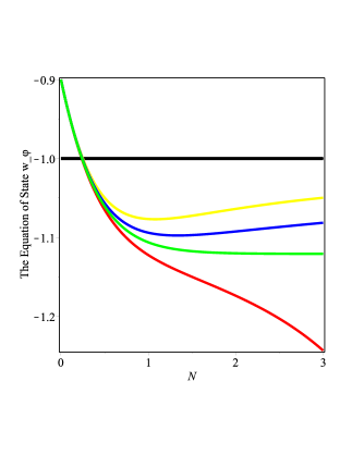
Figure 1: The evolution of the equation of state $w_{\phi}$ with respect to $N$ when $w_{\phi}$ cross the Phantom Line. Fig.2 and Fig.2 are plotted using differential equations (43-45).

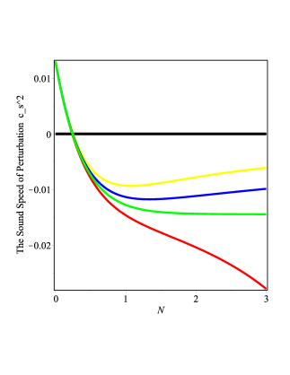
Figure 2: The evolution of $c_{s}^{2}$ with respect to $N$. All the initial conditions are the same as Fig.2. Fig.2 and Fig.2 are plotted under the model of kinetically driven quintessence^♠.

If the equation of state $w_{\phi}$ is near $-1$(so $\gamma_{\phi}\sim 0$) for the kinetically driven quintessence model, we can drop terms of higher order in $\gamma_{\phi}$, and further get a simple differential equation for $\gamma_{\phi}$ with the dependent variable from $N$ to $\Omega_{\phi}$ from Eqs.(43-44):

$$\frac{d\gamma_{\phi}}{d\Omega_{\phi}}=-\frac{2\lambda}{\sqrt{3\Omega_{\phi}}(1-\Omega_{\phi})}-\frac{\gamma_{\phi}}{\Omega_{\phi}(1-\Omega_{\phi})}$$ (47)

We assume that $\lambda$ is approximately constant($=\lambda_{0}$) when $\gamma_{\phi}$ is near $0$, so that the above equation can be solved exactly:

$$\gamma_{\phi}=1+w_{\phi}=-\frac{\sqrt{3}}{3}\lambda_{0}\frac{1-\Omega_{\phi}}{\Omega_{\phi}}\left(ln\left[\frac{1-\sqrt{\Omega_{\phi}}}{1+\sqrt{\Omega_{\phi}}}\right]+\frac{2\sqrt{\Omega_{\phi}}}{1-\Omega_{\phi}}\right)$$ (48)

we have chosen the boundary condition that $\gamma_{\phi}=0$ at $\Omega_{\phi}=0$. Eq.(48) gives the general behaviors of all the kinetic driven quintessence model for all sufficiently flat potentials.

Fig.4 and Fig.4 show how accurate the analytic result(Eq.(48)) is and the tiny differences among different potentials. solid black and red curves are plotted using Eq.(48) directly, and all other curves are numerically plotted from Eqs.(43-45).

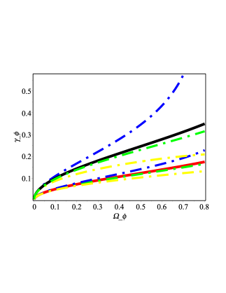
Figure 3: The evolutional behavior of $\gamma_{\phi}$ with respect to $\Omega_{\phi}$. $\lambda_{0}=-0.2,-0.4$ for red and black solid curve respectively. The initial condition when $\Omega_{\phi}=0$ is ($\gamma_{\phi}=0$, $\lambda=-0.2$) and ($\gamma_{\phi}=0$, $\lambda=-0.4$) for the three dashed blue, green and yellow curves around the red and black solid line respectively.

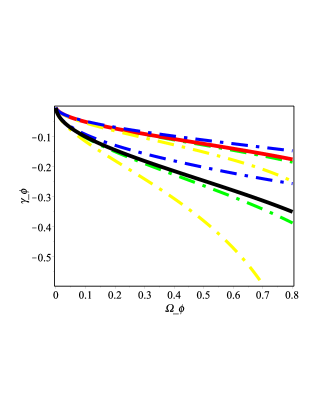
Figure 4: The evolutional behavior of $\gamma_{\phi}$ with respect to $\Omega_{\phi}$. All the initial conditions are the same as Fig.4 except $\lambda_{0}=0.2,0.4$. Solid curve in Fig.4 and Fig.4 are plotted using Eq.(48), all other curves plotted using differential equations (43-45) with different potentials(namely, $\Gamma=1,3/2,2$).

The solid curves(red and black) in Fig.4 and Fig.4 show the general relationship(Eq.(48)) of $\gamma_{\phi}$, $\Omega_{\phi}$ and $\lambda_{0}$. Around each solid curve are the dashed color curves(blue, green and yellow), which are the numerical results of Eqs.(43-45) with different values of $\Gamma$ since different values of $\Gamma$ corresponds to different form of potentials: dashed blue curve for $\Gamma=1$($~{}V_{0}e^{c\phi}$), dashed green curve for $\Gamma=3/2$($~{}V_{0}(\phi+c)^{-2}$) and dashed yellow curve for $\Gamma=2$($V_{0}(\phi+c)^{-1}$). For the dashed green curve, $\Gamma=3/2$ and then $\lambda$ is a constant, so it is easily understood that why the difference between dashed green curve and red(black) solid curve is so small. It also demonstrated that Eq.(48) is valid when the value of $\gamma_{\phi}$ is small. The only difference between Fig.4 and Fig.4 is the opposite values of $\lambda_{0}$. The initial values of $\lambda$ when $\Omega_{\phi}=0$ are $-0.2$(red) and $-0.4$(black) in Fig.4 while $0.2$(red) and $0.4$(black) in Fig.4. We find that the red solid curve and the dashed color curves around it in both Fig.4 and Fig.4 are more close to the Phantom Line($w_{\phi}=-1$). So the smaller the initial value of $|\lambda|$ is(i.e., the more flat the potential is), the less deviation the equation of state $w_{\phi}$ is from $-1$. It is interesting that, for different potentials $~{}V_{0}e^{c\phi}$, $V_{0}(\phi+c)^{-2}$ and $V_{0}(\phi+c)^{-1}$, the state of equation $w_{\phi}$ can larger or less than $-1$, and also can increase or decrease with respect to $\Omega_{\phi}$, only depending on the initial value of $\lambda$(determined by the initial value of $\phi$). Unlike the evolution in Fig.2 and Fig.2, $w_{\phi}$ plotted in Fig.4 and Fig.4 does not cross Phantom Line due to the different choice of the initial conditions.

3.4 Dynamical System for general non-canonical scalar field

In the last subsection of section 3, we consider the general non- canonical scalar field with a lagrangian $L=F(X)-V(\phi)$ filled in a spatially flat Fridmann-Lemaitre-Robertson-Walker(FLRW) cosmology. The motion of this scalar field and the evolution of the universe are described by Eqs.(4-5) and Eq.(7).

In order to obtain the autonomous system we define the variables as follows[40]^†:

$$x=\frac{\sqrt{(2XF_{X}-F)\varsigma}}{\sqrt{3}M_{pl}H},y=\frac{\sqrt{V}}{\sqrt{3}M_{pl}H},\sigma=-\frac{M_{pl}V_{\phi}}{V}\sqrt{\frac{2X}{3(2XF_{X}-F)\varsigma}}sign(\dot{\phi})$$ (49)

Using Eq.(7)and Eq.(49), Eq.(4-5) can be expressed as following dynamical system:

$$\frac{dx}{dN}=\frac{3}{2}[\sigma\varsigma y^{2}-x(w_{k}+1)]+\frac{3}{2}x[(1+w_{b})(1-y^{2})+(w_{k}-w_{b})\varsigma x^{2}]$$ (50)

$$\frac{dy}{dN}=-\frac{3}{2}\sigma xy+\frac{3}{2}y[(1+w_{b})(1-y^{2})+(w_{k}-w_{b})\varsigma x^{2}]$$ (51)

$$\frac{d\sigma}{dN}=-3\sigma^{2}x(\Gamma-1)+\frac{3\sigma[2\Xi(w_{k}+1)+w_{k}-1]}{2(2\Xi+1)(w_{k}+1)}(w_{k}+1-\frac{\sigma y^{2}}{\varsigma x})$$ (52)

where

$$w_{k}=\gamma_{k}-1=\frac{F}{2XF_{X}-F},~{}w_{\phi}=\frac{p_{\phi}}{\rho_{\phi}}=\frac{w_{k}\varsigma x^{2}-y^{2}}{\varsigma x^{2}+y^{2}},~{}\Omega_{\phi}=\varsigma x^{2}+y^{2},~{}\Xi=XF_{XX}/F_{X}$$ (53)

From Eq.(53), we can get following relationships:

$$x^{2}=\frac{\gamma_{\phi}\varsigma}{\gamma_{k}}\Omega_{\phi},~{}~{}~{}~{}y^{2}=\frac{\gamma_{k}-\gamma_{\phi}}{\gamma_{k}}\Omega_{\phi}$$ (54)

Using Eqs.(53-54), the dynamical system Eqs.(50-52) can be rewritten with the variables $(\Omega_{\phi},\gamma_{\phi},\sigma)$ related with observable quantities:

$$\frac{d\Omega_{\phi}}{dN}=3(\gamma_{b}-\gamma_{\phi})\Omega_{\phi}(1-\Omega_{\phi})$$ (55)

$$\frac{d\gamma_{\phi}}{dN}=3\left[\varsigma\gamma_{\phi}(\gamma_{\phi}-1-\frac{1}{2\Xi+1})+2\sigma\sqrt{\frac{\varsigma\Omega_{\phi}\gamma_{\phi}}{\gamma_{k}}}\frac{(\gamma_{k}-\gamma_{\phi})(\Xi+1)}{(2\Xi+1)\gamma_{k}}\right]$$ (56)

$$\frac{d\sigma}{dN}=-3\sigma\left(\sigma(\Gamma-1)\sqrt{\frac{\varsigma\Omega_{\phi}\gamma_{\phi}}{\gamma_{k}}}+(\frac{1}{2\Xi+1}-\frac{\gamma_{k}}{2})\left[\sigma\sqrt{\frac{\varsigma\Omega_{\phi}\gamma_{\phi}}{\gamma_{k}}}(\frac{1}{\gamma_{k}}-\frac{1}{\gamma_{\phi}})+1\right]\right)$$ (57)

Beside the three variables $(\Omega_{\phi},\gamma_{\phi},\sigma)$, there are other quantities in Eqs.(56-57) which are not constant: $\Xi,\gamma_{k}$ and $\Gamma$. We know that $\gamma_{\phi}=p_{\phi}/\rho_{\phi}+1=\gamma_{\phi}(X,\phi)=\gamma_{\phi}(\dot{\phi},\phi)$ and $\sigma=\sigma(\dot{\phi},\phi)$. So generally speaking, we can obtain the expressions of $\phi=\phi(\gamma_{\phi},\sigma)$ and $\dot{\phi}=\dot{\phi}(\gamma_{\phi},\sigma)$. For the parameters $\Xi,\gamma_{k}$ and $\Gamma$, we know $\Xi=\Xi(\dot{\phi}),\gamma_{k}=\gamma_{k}(\dot{\phi})$ and $\Gamma=\Gamma(\phi)$, so they can be expressed as $\Xi(\gamma_{\phi},\sigma),\gamma_{k}(\gamma_{\phi},\sigma)$ and $\Gamma(\gamma_{\phi},\sigma)$. Therefore, Eqs.(55-57) could in principal be a dynamical autonomous system though it is actually quite complicated.

We take two simple examples to check the correctness of Eqs.(55-57) and study its properties. First example is, we know that general non-canonical scalar field with lagrangian $F(X)-V(\phi)$ will reduce to (phantom) quintessence if $F(X)=\varsigma X$, and Eqs.(56-57) should reduce to Eqs.(19-20)(Eq.(55) has the same form with Eq.(18)). $F(X)=\varsigma X$ makes $\Xi=0$, $\gamma_{k}=2$ and $\sigma=\sqrt{\frac{2}{3}}\lambda$, then we found Eqs.(56-57) have the same form with Eqs.(19-20).

Another example is that, if the potential $V(\phi)=-1$ in K-essence and the Potential $V(\phi)=0$ in general non-canonical scalar field, these two scalar field models will have the same form of lagrangian $L=F(X)$, then both will reduce to the so-called purely kinetic united model[41, 42]. In this case, $d\lambda/dN=0$ and $d\sigma/dN=0$, then both Eqs.(38-40) and Eqs.(55-57) will reduce to a two-dimensional dynamical system as follows:

$$\frac{d\Omega_{\phi}}{dN}=3(\gamma_{b}-\gamma_{\phi})\Omega_{\phi}(1-\Omega_{\phi})$$ (58)

$$\frac{d\gamma_{\phi}}{dN}=3\gamma_{\phi}(\gamma_{\phi}-1-\frac{1}{2\Xi+1})$$ (59)

For the case of purely kinetic united model $L=F(X)$, we know from Eq.(49) and Eq.(53) that $\gamma_{\phi}$ is a function of $X$, $\gamma_{\phi}=\gamma_{k}=\frac{F}{2XF_{X}-F}$. In the meantime, $\Xi$ is also a function of $X$ because $\Xi=XF_{XX}/F_{X}=(xF^{\prime\prime}-F^{\prime})/2F^{\prime}$. So generally speaking, $\Xi$ can be expressed as a function of $\gamma_{\phi}$. Then the system of Eqs.(58-59) could be a two-dimensional autonomous dynamical system. For some special cases of $F(X)$, we can even get the exact solution for $\Omega_{\phi}$ and $\gamma_{\phi}$. We take two examples to illustrate our viewpoints.

The most simple is the case that $\Xi$ is a constant. We know that $\Xi=\frac{2-\alpha}{2(\alpha-1)}=\frac{XF_{XX}}{F_{X}}$, we can integrate and get the form for $F(X)$:

$$F(X)=CX^{\frac{\alpha}{2(\alpha-1)}}+X_{0}$$ (60)

We can also get the exact solution for $\Omega_{\phi}$ and $\gamma_{\phi}$ from Eqs.(58-59):

$$\gamma_{\phi}(N)=\frac{1}{c_{3}e^{3\alpha N}+1/\alpha},~{}~{}\Omega_{\phi}(N)=\frac{1}{c_{4}(c_{3}\alpha e^{3\alpha N}+1)^{-1}e^{3(\alpha-\gamma_{b})N}+1}$$ (61)

where $\alpha=1+\frac{1}{2\Xi+1}$, $C$, $X_{0}$, $c_{3}$ and $c_{4}$ are the integral constants. If we set the equation of state of dark energy $\gamma_{\phi}(0)=\gamma_{0}$ and energy density of dark energy $\Omega_{\phi}(0)=\Omega_{0}$ at present $N=0$, we then get $c_{3}=\frac{\alpha-\gamma_{0}}{\alpha\gamma_{0}}$ and $c_{4}=\frac{\alpha(1-\Omega_{0})}{\Omega_{0}\gamma_{0}}$.

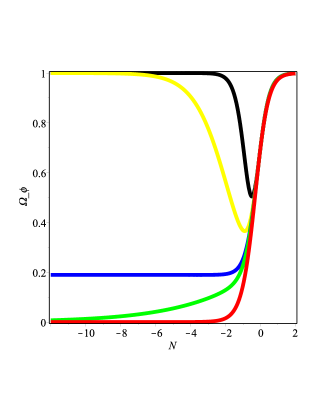
Figure 5: The evolution of $\Omega_{\phi}$ with respect to $N$ when $F(X)=CX^{\frac{\alpha}{2(\alpha-1)}}+X_{0}$ and $\gamma_{b}=1$, initial condition is chosen as $\gamma_{\phi}=0.1$ and $\Omega_{\phi}=0.7$ at present($N=0$). The color lines from the top to the bottom are plotted with $\alpha=0.3,~{}0.9,~{}1.0,~{}4/3,~{}2.0$.

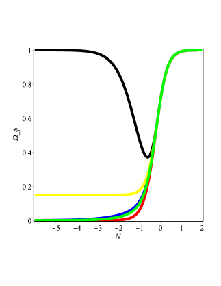
Figure 6: The evolution of $\Omega_{\phi}$ with respect to $N$ when $F(X)=CX^{\frac{\alpha}{2(\alpha-1)}}+X_{0}$. The initial condition and the values of the parameter $\alpha$ are the same as Fig.6 except $\gamma_{b}=4/3$. Fig.6 and Fig.6 are plotted using Eq.(61).

For the cosmic evolution in very early time, $N$ is negative and $|N|$ is very large, we get $\gamma_{\phi}\approx\alpha$ from Eq.(61), and then energy density of scalar field will behave as $\rho_{\phi}\sim a^{-3\alpha}$.

For the cosmic evolution in late time, $N$ is positive and very large, $\gamma_{\phi}\approx 0$ and $\Omega_{\phi}\approx 1$, scalar field behaves as the cosmological constant.

Noted that there is only kinetic term in the lagrangian which gives the cosmological constant solution. Moreover,

From Eq.(61) that $\Omega_{\phi}$ might not be 0 in the very early time. Its value depends on the value of $\alpha$ comparing with the value of $\gamma_{b}$($\gamma_{b}=1$ for matter and $\gamma_{b}=4/3$ for radiation).

We have plotted the evolution of $\Omega_{\phi}$ with respect to $N$ for different $\alpha$ and different $\gamma_{b}$ in Fig.6 and Fig.6, and

Fig.6 and Fig.6 show that the value of $\Omega_{\phi}$ in the very early time could be 1, 0 or a positive constant which is less then 1.

When $N\rightarrow-\infty$, we can get $\Omega_{\phi}(N)\approx 1/(c_{4}e^{3(\alpha-\gamma_{b})N}+1)$ from Eq.(61).

Then $\Omega_{\phi}\rightarrow 1$ for $\alpha>\gamma_{b}$, $\Omega_{\phi}\rightarrow 1/(c_{4}+1)$ for $\alpha=\gamma_{b}$ and $\Omega_{\phi}\rightarrow 0$ for $\alpha<\gamma_{b}$.

If $\Omega_{\phi}>0$ in very early time, it would be very interesting to investigate its impact on the evolutional history of early universe.

The second case is the lagrangian as follows:

$$F(X)=A_{1}\sqrt{X}-A_{2}X^{\beta}$$ (62)

where $A_{1}$, $A_{2}$, and $\beta$ are constants. This form of $F(X)$ was proposed in [41, 43]. From Eq.(53), we can get that $\Xi=(2\beta-\gamma_{\phi})/2\gamma_{\phi}$, then dynamical system Eqs.(58-59) becomes the following equations:

$$\frac{d\Omega_{\phi}}{dN}=3(\gamma_{b}-\gamma_{\phi})\Omega_{\phi}(1-\Omega_{\phi})$$ (63)

$$\frac{d\gamma_{\phi}}{dN}=3\gamma_{\phi}(\frac{2\beta-1}{2\beta}\gamma_{\phi}-1)$$ (64)

Solving above differential equations, we obtain the following exact solution for $\gamma_{\phi}$ and $\Omega_{\phi}$:

$$\gamma_{\phi}(N)=\frac{1}{c_{5}e^{3N}+1/\eta},~{}~{}\Omega_{\phi}(N)=\frac{1}{c_{6}(c_{5}\eta e^{3N}+1)^{-\eta}e^{3(\eta-\gamma_{b})N}+1}$$ (65)

where $c_{5}$ and $c_{6}$ are the integral constants, $\eta=\frac{2\beta}{2\beta-1}$, is also a constant. Eq.(65) is very similar but a little different with the evolution described in Eq.(61):

$$\gamma_{\phi}(N)=\frac{1}{c_{3}e^{3\alpha N}+1/\alpha},~{}~{}\Omega_{\phi}(N)=\frac{1}{c_{4}(c_{3}\alpha e^{3\alpha N}+1)^{-1}e^{3(\alpha-\gamma_{b})N}+1}$$

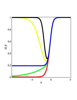
Figure 7: The evolution of $\Omega_{\phi}$ with respect to $N$ when $F(X)=A_{1}\sqrt{X}-A_{2}X^{\beta}$ and $\gamma_{b}=1$, initial condition is chosen as $\gamma_{\phi}=0.1$ and $\Omega_{\phi}=0.7$ at present($N=0$). The color lines from the top to the bottom are plotted with $\eta=0.3,~{}0.9,~{}1.0,~{}4/3,~{}2.0$.

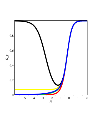
Figure 8: The evolution of $\Omega_{\phi}$ with respect to $N$ when $F(X)=A_{1}\sqrt{X}-A_{2}X^{\beta}$. The initial condition and the values of the parameter $\eta$ are the same as Fig.8 except $\gamma_{b}=4/3$. Fig.8 and Fig.8 are plotted using Eq.(65).

For the cosmic evolution in very early time, $N$ is negative and $|N|$ is very large, we get $\gamma_{\phi}\approx\eta=2\beta/(2\beta-1)$ from Eq.(65). The scalar field will mimic the evolution of matter with zero pressure $\rho\sim a^{-3}$ in the limit of $\beta\rightarrow\infty$. For the cosmic evolution in late time, $N$ is very large, $\gamma_{\phi}\approx 0$ and $\Omega_{\phi}\approx 1$, scalar field behaves as the cosmological constant. So it is the second case that a lagrangian without a potential term gives the cosmological constant solution. Moreover, we know from Eq.(65) that $\Omega_{\phi}$ might not be 0 in the very early time. It depends on the value of $\eta$ comparing with the value of $\gamma_{b}$($\gamma_{b}=1$ for matter and $\gamma_{b}=4/3$ for radiation). When $N\rightarrow-\infty$, we can get $\Omega_{\phi}(N)\approx 1/(c_{6}e^{3(\eta-\gamma_{b})N}+1)$ from Eq.(65). Then $\Omega_{\phi}\rightarrow 1$ for $\eta>\gamma_{b}$, $\Omega_{\phi}\rightarrow 1/(c_{6}+1)$ for $\eta=\gamma_{b}$ and $\Omega_{\phi}\rightarrow 0$ for $\eta<\gamma_{b}$. In this case, it will be interesting to investigate the impact of the scalar field on the evolutional history of the early universe. We have plotted the evolution of $\Omega_{\phi}$ with respect to $N$ for different $\eta$ and different $\gamma_{b}$ in Fig.8 and Fig.8, and it is shown that the value of $\Omega_{\phi}$ in the very early time can actually be 1, 0 or an arbitrary positive constant which is less than 1.

4 Cosmological Implications and Conclusion

The main purpose of the paper is not to analyze the dynamical behavior about different scalar fields in detail, so we will not investigate the detailed critical points and their stable properties for each dynamical system. What we want to focus on is about the dynamical system itself.

4.1 Variables $(x,y)$ vs observable quantities $(\gamma_{\phi},\Omega_{\phi})$

Dynamical variables ($x,y$) in the previous papers are about the scalar field and its first derivative. Though for some scalar field models(quintessence or phantom quintessence), the combination of variables ($x,y$) has certain meaning, namely , $y^{2}\pm x^{2}=\Omega_{\phi}$, but generally speaking, these dynamical variables have no direct cosmological meaning, and the autonomous system for $dx/dN$ and $dy/dN$ also varies from different models. Authors studied dynamical properties of scalar field based on quantities $(\gamma_{\phi},\Omega_{\phi})$ instead of variables $(x,y)$[21, 22, 23, 24, 25, 26, 27, 28, 30]. It is more convenient if we change the variables from $(x,y)$ to observable quantities $(\gamma_{\phi},\Omega_{\phi})$. Firstly, $(\gamma_{\phi},\Omega_{\phi})$ are directly related to the observable quantities and also about the properties of dark energy. Analyzing the system based on $(\gamma_{\phi},\Omega_{\phi})$, we can figure out how the equation of state of dark energy $w_{\phi}$ and the density parameter $\Omega_{\phi}$ evolve. Secondly, though the form of autonomous system for $dx/dN$ and $dy/dN$ are completely different for different models, but it is quite interesting that the function for $d\Omega_{\phi}/dN$ has the same expression in quintessence, tachyon, k-essence and general non-canonical scalar field model(i.e., Eq.(18),Eq.(27),Eq.(38),Eq.(55)) as follows:

$$\frac{d\Omega_{\phi}}{dN}=3(\gamma_{b}-\gamma_{\phi})\Omega_{\phi}(1-\Omega_{\phi})$$ (66)

The only difference is the form of function $d\gamma_{\phi}/dN$. In fact, it is a well-known fact that Eq.(66) holds for all non-coupled dark energy models as long as they satisfy the following equations:

$$H^{2}=\frac{1}{3M^{2}_{pl}}(\rho_{b}+\rho_{de}),~{}\dot{\rho}_{i}+3H(p_{i}+\rho_{i})=0$$ (67)

where subscript $i$ denotes each energy component such as dark energy, matter or radiation. If we set $\gamma_{de}=w_{de}+1=p_{de}/\rho_{de}+1$ and $\Omega_{de}=\rho_{de}/3M^{2}_{pl}H^{2}$, Eq.(66) can be derived from Eq.(67). So the dark energy density parameter $\Omega_{\phi}$ obeys the same differential equation( namely Eq.(66)) independent on the scalar field models considered whenever the dark energy is uncoupled in GR frame. For example, the authors got the same equation even for the purely kinetic coupled gravity model which modified the standard general relativity action through the addition of a coupling between functions of the metric and kinetic terms of a free scalar field[44](Eq.(28) in this paper and $\gamma_{b}$ is taken as 1).

We can conclude from Eq.(66) that there are only three possible destinies(three types of critical points) for $\Omega_{de}$ to be in these models, namely $\Omega_{de}=0$, $\Omega_{de}=1$ and the case $\gamma_{de}=\gamma_{b}$ where the value of $\Omega_{\phi}$ is determined by other equation in the dynamical system. The cases of $\Omega_{de}=0$ or $\Omega_{de}=1$ are completely opposite destinies, corresponding to the universe completely dominated only by the scalar field or by the barotropic fluid. Generally speaking, we can obtain $0<\Omega_{de}<1$ for the case of $\gamma_{de}=\gamma_{b}$. However, for this scaling solution, the equation of state of dark energy $w_{de}$ is the same as the equation of state of barotropic fluid $w_{b}$, so there is no accelerating expansion. Since the observation suggested that we are living in an accelerated expanding universe with $\Omega_{de}\sim 0.7$, none of these three destinies correspond to the present universe we observed. This could be considered as a clue for the possibility of the interaction between dark energy and other barotropic fluids(see [45] for such model) if we want to solve or at least alleviate the cosmological coincidence problem without fine-tunings. This result is valid for not only all the non- coupled dark energy models, but also for many modified gravity models as long as the energy density and the pressure of dark energy or effective dark energy satisfy the continuity equation Eq.(67). However, we should emphasize that our result is not new, there are many works on the study of interacting model of dark energy model[21, 22, 31, 32, 33].

4.2 Two-Dimensional vs Three-Dimensional dynamical autonomous system

Another important thing we want to emphasize is that, it is more reasonable and more scientific to investigate the dynamical behaviors of a dark energy model under the three-dimensional autonomous system rather than the two-dimensional system. Firstly, the two-dimensional dynamical autonomous system is just a specific case when the potential takes a special form. if we want to completely study the general dynamical properties of a dark energy model, we need to study the system beyond a special potential. Then we can find more critical points than the ones found in a two-dimensional system. We therefore are able to analyze which critical points are possessed by a class of dark energy models and which ones exist only due to the concrete potentials. The method studying the three-dimensional dynamical autonomous system beyond one special potential is originated for the quintessence [11, 46] and then developed to other dark energy models [12, 13, 14, 15, 16, 17, 18, 19, 45, 20]. Here we extend this method to the more general scalar field models in Section 3. Secondly, more stable attractors can be found in terms of three dimensional autonomous system. For example, a new critical point is found only in three dimensional dynamical system of power-law kinetic quintessence, which corresponds to the dark energy dominated universe($\Omega_{\phi}=1$) where power-law kinetic quintessence behaves as an cosmological constant with the sound speed $c_{s}^{2}$ being 0[65]. Thirdly, from the viewpoint of chaos theory, the dynamical properties of three-dimensional autonomous system is more fruitful than the two-dimensional system. According to the Poincar$\acute{e}$ -Bendixson theorem, chaos does not exist in any two-dimensional autonomous dynamical system[47, 48] but could be possible in three-dimensional autonomous dynamical system. For a number of three-dimensional systems, such as the famous three-dimensional Lorenz equations which is a model describing the atmospheric convection [49], there exist chaos for certain values of the parameters.

4.3 Stable attractors vs chaotic behaviors

The studies of chaotic dynamics in cosmological models has a long story. Chaotic properties had reported in spatially closed scalar field FRW cosmological models [50, 51, 52, 53, 54, 55], spatially flat FRW cosmological model with two or more scalar fields [56, 57], Bianchi IX universe [58, 59], Bianchi I universe[60] and the mixmaster universe[61]. It would be very interesting and also a big challenge for the theoretical study of dark energy if the dynamical systems we consider here(i.e., Eqs.(18-20),Eqs.(27-29),Eqs.(38-40) and Eqs.(55-57) ) exist the chaotic properties. Then the evolution of $\Omega_{\phi}$ and $\gamma_{\phi}$ will be very sensitive to the initial condition, and therefore predicting their evolution in future becomes totally impossible. However, it is proved that there is no chaotic behavior in spatially flat single scalar field FRW cosmological models[62, 63]. Since for the spatially flat case with $k=0$, the dynamical system can be described by a three-dimensional autonomous system with a set of variables $(H,\phi,\dot{\phi})$ under a Hamiltonian constraint, so the dynamical system is actually a two-dimensional autonomous system($a$ and $\dot{a}$ appear only in the combination $H=\dot{a}/a$)[64]. We know that for the two-dimensional autonomous systems, there are no enough degrees of freedom to exist chaos, so this proved no-chaotic dynamics in the spatially flat scalar field FRW cosmological model. However, we noted that this result is obtained in the absence of matter and radiation. This may be the case in the very early time when our universe is undergoing an inflation era and completely dominated by the scalar field. However, for the study of dark energy of late-time cosmic acceleration, the component of matter is comparable with the density of dark energy and should not be ignored when we investigate the dynamical behavior of scalar field. In the presence of matter, scale factor $a$ will reappear in the dynamical system beside the variables $(H,\phi,\dot{\phi})$, and then the system can not be reduced to two-dimensional autonomous dynamical system any more. So here we argue that, beside the ordinary attractors(such as dark energy dominated solution, de-Sitter like solution and scaling solution), it is still possible for the chaotic behavior in spatially flat single scalar field FRW cosmological models in the presence of matter. It is very like the case of spatially non-flat($k\neq 0$) single scalar field FRW cosmological models where the dynamical system can not be reduced to two-dimensional autonomous dynamical system too. What we argued here is also supported by the equations in section 3( i.e., Eqs.(18-20), Eqs.(27-29), Eqs.(38-40) and Eqs.(55-57)), which described three-dimensional autonomous dynamical systems. However, we are not sure whether there truly exist the chaotic behavior in spatially flat scalar field FRW cosmological models now, to find the chaotic behavior is beyond the scope of this paper, it should be investigated in future.

5 Acknowledgement

We owes the great improvement of this paper to the anonymous referees. This work is partly supported by Chinese National Nature Science Foundation under Grant No.11333001, No.11433003, 973 Program No.2014CB845704 and Shanghai Science Foundations 13JC1404400. This work is also supported by Shanghai Normal University.

References

- [1] B. Ratra and P. J. E. Peebles, Phys. Rev. D37, 3406 (1988)
- [2] E. J. Copeland, M. Sami and S. Tsujikawa, Int. J. Mod. Phys. D15, 1753 (2006)
- [3] M. Li, X. D. Li, S. Wang and Y. Wang, Commun. Theor. Phys56, 525-604 (2011)
- [4] A. A. Coley,
- [5] C. Xu, E. N. Saridakis and G. Leon, JCAP 0904, 001 (2009)
- [6] G. Leon and E. N. Saridakis, JCAP1303, 025 (2013)
- [7] G. Leon, J. Saavedra and E. N. Saridakis, Class.Quant.Grav.30, 135001 (2013)
- [8] C. R. Fadragas, G. Leon and E. N. Saridakis, Class. Quantum Grav.31, 075018 (2014)
- [9] J. M. Aguirregabiria, L. P. Chimento and R. Lazkoz, Phys. Lett. B631, 93-99 (2005)
- [10] A. R. Liddle, Paul Parsons and J. D. Barrow, Phys. Rev. D50, 7222-7232 (1994)
- [11] W. Fang, Y. Li, K. Zhang and H. Q. Lu, Class. Quantum Grav.26, 155005 (2009)
- [12] I. Quiros, T. Gonzalez, D. Gonzalez, Y. Napoles, R. Garcia-Salcedo and C. Moreno, Class. Quant. Grav.27, 215021(2010)
- [13] Y. Leyva, D. Gonzalez, T.Gonzalez, T. Matos and I. Quiros, Phys. Rev. D80, 044026 (2009)
- [14] T. Matos, J. R. Luevano, I. Quiros, L. A. Urena-Lopez and J. A. Vazquez, Phys. Rev. D80, 123521 (2009)
- [15] K. Xiao and J. Y. Zhu, Phys. Rev. D83, 083501 (2011)
- [16] D. Escobar, C. R. Fadragas, G. Leon and Y. Leyva, Class. Quantum Grav.29, 175005 (2012)
- [17] D. Escobar, C. R. Fadragas, G. Leon and Y. Leyva, Class. Quantum Grav.29, 175006 (2012)
- [18] G. Leon, Y. Leyva and J. Socorro, arXiv:1208.0061
- [19] S. del Campo, C. R. Fadragas, R. Herrera, C. Leiva, G. Leon and J. Saavedra, Phys. Rev. D88, 023532 (2013)
- [20] G. Otalora, Phys. Rev. D88, 063505 (2013)
- [21] L. P. Chimento, A. S. Jakubi and D. Pavon, Phys. Rev. D67, 087302 (2003)
- [22] L. P. Chimento, A. S. Jakubi, D. Pavon and W. Zimdahl, Phys. Rev. D67, 083513 (2003)
- [23] J. G. Hao and X. Z. Li, Phys. Rev. D70, 043529 (2004)
- [24] R. J. Scherrer and A. A. Sen, Phys. Rev. D77, 083515 (2008)
- [25] G. Gupta, S. Majumdar and A. A. Sen, MNRAS420, 1309 (2012)
- [26] S. Dutta and R. J. Scherrer, Phys. Lett.B704, 265-269 (2011)
- [27] W. Fang and H. Q. Lu, Eur. Phys. J. C68, 567-572 (2010)
- [28] N. C. Devi, T. R. Choudhury and A. A. Sen, MNRAS432, 1513-1524 (2013)
- [29] X. M. Chen and Y. G. Gong, arXiv:1309.2044
- [30] Y. G. Gong, arXiv:1401.1959
- [31] L. Amendola, Phys. Rev. D62, 043511 (2000)
- [32] R. Curbelo, T. Gonzalez, Genly Leon and I. Quiros, Class. Quant. Grav. 23, 1587 (2006)
- [33] T. Gonzalez, G. Leon and I. Quiros, Class. Quant. Grav. 23, 3165 (2006)
- [34] R. J. Yang and X. T. Gao, Chin. Phys. Lett.26, 089501 (2009)
- [35] N. Tamanini, arXiv:1401.6339
- [36] T. Chiba, T. Okabe and M. Yamaguchi, Phys. Rev. D62, 023511 (2000)
- [37] R. J. Yang and X. T. Gao, Class. Quant. Grav.28, 065012 (2011)
- [38] J. Garriga and V.F. Mukhanov, Phys. Lett. B458, 219-225 (1999)
- [39] A. Vikman, Phys. Rev. D71, 023515 (2005)
- [40] J. De-Santiago, J. L. Cervantes-Cota and D. Wands, Phys. Rev. D87, 023502(2013)
- [41] R. J. Scherrer, Phys. Rev. Lett.93, 011301 (2004)
- [42] J. L. Cervantes-Cota, A. Aviles and J. De-Santiago, AIP Conf. Proc.1548, 299-313 (2013)
- [43] L. P. Chimento, Phys. Rev. D69, 123517 (2004)
- [44] G. Gubitosia and E. V.Linder, Phy. Lett. B703, 113-118 (2011)
- [45] G. Otalora, JCAP07, 044 (2013)
- [46] S. Y. Zhou, Phys. Lett. B660, 7-12(2008)
- [47] S. Wiggins, (New York: Springer, 1990)
- [48] F. Zhang and J. Heidelz, Nonlinearity10, 1289-1303(1997)
- [49] E. N. Lorenz, Journal of Atmospheric Sciences20, 130(1963)
- [50] S. Blanco, G. Domenech, C. El Hasi, and O. A. Rosso, Gen.Rel.Grav.26, 1131-1143 (1994)
- [51] E. Calzetta and C. El Hasi, Class. Quant. Grav.10, 1825 (1993)
- [52] E. Calzetta and C. El Hasi, Phys. Rev. D51, 2713(1995)
- [53] A. V. Toporensky, Int.J.Mod.Phys. D8, 739-750 (1999)
- [54] S. E. Jors and T. J. Stuchi, Phys.Rev. D68, 123525 (2003)
- [55] G. Lukes-Gerakopoulos, S. Basilakos and G. Contopoulos, Phys. Rev. D77, 043521 (2008)
- [56] N. J.Cornish and J. J. Levin, Phys. Rev. D53, 3022-3032 (1996)
- [57] R. Easther and Kei-ichi Maeda, Class. Quant. Grav.16, 1637-1652 (1999)
- [58] S. Fay and T. Lehner, Gen.Rel.Grav.37, 1097-1117 (2005);
- [59] E. J. Kim and S. Kawai,Phys. Rev. D87, 083517 (2013)
- [60] J. H. Chen and Y. J. Wang, Chinese Phys.14, 1282 (2005)
- [61] N. J. Cornish and J. J. Levin, Phys. Rev. Lett.78, 998-1001 (1997)
- [62] E. Gunzig, L. Brenig, A. Figueiredo and T.M. Rocha Filho, Mod. Phys. Lett. A15, 1363-1368 (2000)
- [63] V. Faraoni, M. N. Jensen and S. A. Theuerkauf, Class.Quant.Grav.23, 4215-4230 (2006)
- [64] O. Hrycyna, , doctoral dissertation (2011)
- [65] W. Fang, H. Tu, Y. Li, J. S. Huang and C. G. Shu, Phy. Rev. D89, 123514 (2014)