Sequential Quasi-Monte Carlo

Abstract

We derive and study SQMC (Sequential Quasi-Monte Carlo), a class of algorithms obtained by introducing QMC point sets in particle filtering. SQMC is related to, and may be seen as an extension of, the array-RQMC algorithm of L’Ecuyer et al., (2006). The complexity of SQMC is $\mathcal{O}(N\log N)$, where $N$ is the number of simulations at each iteration, and its error rate is smaller than the Monte Carlo rate $\mathcal{O}_{P}(N^{-1/2})$. The only requirement to implement SQMC is the ability to write the simulation of particle $\mathbf{x}_{t}^{n}$ given $\mathbf{x}_{t-1}^{n}$ as a deterministic function of $\mathbf{x}_{t-1}^{n}$ and a fixed number of uniform variates. We show that SQMC is amenable to the same extensions as standard SMC, such as forward smoothing, backward smoothing, unbiased likelihood evaluation, and so on. In particular, SQMC may replace SMC within a PMCMC (particle Markov chain Monte Carlo) algorithm. We establish several convergence results. We provide numerical evidence that SQMC may significantly outperform SMC in practical scenarios.

Key-words: Array-RQMC; Low discrepancy; Particle filtering; Quasi-Monte Carlo; Randomized Quasi-Monte Carlo; Sequential Monte Carlo

1 Introduction

Sequential Monte Carlo (SMC, also known as particle filtering) is a class of algorithms for computing recursively Monte Carlo approximations of a sequence of distributions $\pi_{t}(\mathrm{d}\mathbf{x}_{t})$, $t\in 0{:}T$, $0{:}T=\{0,\ldots,T\}$. The initial motivation of SMC was the filtering of state-space models (also known as hidden Markov models); that is, given a latent Markov process $(\mathbf{x}_{t})$, observed imperfectly as e.g. $\mathbf{y}_{t}=f(\mathbf{x}_{t})+\mathbf{\epsilon}_{t}$, recover at every time $t$ the distribution of $\mathbf{x}_{t}$ given the data $\mathbf{y}_{0:t}=(\mathbf{y}_{0},\ldots,\mathbf{y}_{t})$. SMC’s popularity stems from the fact it is the only realistic approach for filtering and related problems outside very specific cases (such as the linear Gaussian model). Recent research has further increased interest in SMC, especially in Statistics, in at least two directions. First, several papers (Neal,, 2001; Chopin,, 2002; Del Moral et al.,, 2006) have extended SMC to non-sequential problems; that is, to sample from distribution $\pi$, one applies SMC to some artificial sequence $\pi_{t}$ that ends up at $\pi_{T}=\pi$. In certain cases, such an approach outperforms MCMC (Markov chain Monte Carlo) significantly. Second, the seminal paper of Andrieu et al., (2010) established that SMC may be used as a proposal mechanism within MCMC, leading to so called PMCMC (particle MCMC) algorithms. While not restricted to such problems, PMCMC is the only possible approach for inference in state-space models such that the transition kernel of $(\mathbf{x}_{t})$ may be sampled from, but does not admit a tractable density. Excitement about PMCMC is evidenced by the 30 papers or so that have appeared in the last two years on possible applications and extensions.

Informally, the error rate of SMC at iteration $t$ is $C_{t}N^{-1/2}$, where $C_{t}$ is some function of $t$. There has been a lot of work on SMC error rates (e.g. Del Moral,, 2004), but it seems fair to say that most of it has focussed on the first factor $C_{t}$; that is, whether to establish that the error rate is bounded uniformly in time, $C_{t}\leq C$, or to reduce $C_{t}$ through more efficient algorithmic designs, such as better proposal kernels or resampling schemes.

In this work, we focus on the second factor $N^{-1/2}$, i.e. we want the error rate to converge quicker relative to $N$ than the standard Monte Carlo rate $N^{-1/2}$. To do so, we adapt to the SMC context ideas borrowed from QMC (Quasi-Monte Carlo); that is, the idea of replacing random numbers by low discrepancy point sets.

The following subsections contain very brief introductions to SMC and QMC, with an exclusive focus on the concepts that are essential to follow this work. For a more extensive presentation of SMC, the reader is referred to the books of Doucet et al., (2001), Del Moral, (2004) and Cappé et al., (2005), while for QMC and RQMC, see Chapter 5 of Glasserman, (2004), Chapters 5 and 6 of Lemieux, (2009), and Dick and Pillichshammer, (2010).

1.1 Introduction to SMC

As already mentioned, the initial motivation of SMC is the sequential analysis of state-space models; that, is models for a Markov chain $(\mathbf{x}_{t})$ in $\mathcal{X}\subseteq\mathbb{R}^{d}$,

$$\mathbf{x}_{0}\sim f^{X}_{0}(\mathbf{x}_{0}),\quad\mathbf{x}_{t}|\mathbf{x}_{t-1}\sim f^{X}(\mathbf{x}_{t}|\mathbf{x}_{t-1}),$$

which is observed only indirectly through some $\mathbf{y}_{t}$, with density $\mathbf{y}_{t}|\mathbf{x}_{t}\sim f^{Y}(\mathbf{y}_{t}|\mathbf{x}_{t})$.

This kind of model arises in many areas of science: in tracking for instance, $\mathbf{x}_{t}$ may be the position of a ship (in two dimensions) or a plane (in three dimensions), and $\mathbf{y}_{t}$ may be a noisy angular observation (radar). In Ecology, $\mathbf{x}_{t}$ would be the size of a population of bats in a cave, and $\mathbf{y}_{t}$ would be $\mathbf{x}_{t}$ plus noise. And so on.

The most standard inferential task for such models is that of filtering; that is, to recover iteratively in time $t$, $p(\mathbf{x}_{t}|\mathbf{y}_{0:t})$, the distribution of $\mathbf{x}_{t}$, given the data collected up time $t$, $\mathbf{y}_{0:t}=(\mathbf{y}_{0},\ldots,\mathbf{y}_{t})$. One may also be interested in smoothing, $p(\mathbf{x}_{0:t}|\mathbf{y}_{0:t})$, or likelihood evaluation, $p(\mathbf{y}_{0:t})$, notably when the model depends on a fixed parameter $\theta$ which should be learnt from the data.

A simple Monte Carlo approach to filtering is sequential importance sampling: choose an initial distribution $m_{0}(\mathrm{d}\mathbf{x}_{0})$, a sequence of Markov kernels $m_{t}(\mathbf{x}_{t-1},\mathrm{d}\mathbf{x}_{t})$, $t\geq 1$, then simulate $N$ times iteratively from these $m_{t}$’s, $\mathbf{x}_{0}^{n}\sim m_{0}(\mathrm{d}\mathbf{x}_{0})$, $\mathbf{x}_{t}^{n}|\mathbf{x}_{t-1}^{n}\sim m_{t}(\mathbf{x}_{t-1}^{n},\mathrm{d}\mathbf{x}_{t})$, and reweight ‘particle’ (simulation) $\mathbf{x}_{t}^{n}$ as follows: $w_{0}^{n}=G_{0}(\mathbf{x}_{0}^{n})$, $w_{t}^{n}=w_{t-1}^{n}\times G_{t}(\mathbf{x}_{t-1}^{n},\mathbf{x}_{t}^{n})$, where the weight functions $G_{t}$ are defined as

$$G_{0}(\mathbf{x}_{0})=\frac{f^{Y}(\mathbf{y}_{0}|\mathbf{x}_{0})f^{X}_{0}(\mathbf{x}_{0})}{m_{0}(\mathbf{x}_{0})},\quad G_{t}(\mathbf{x}_{t-1},\mathbf{x}_{t})=\frac{f^{Y}(\mathbf{y}_{t}|\mathbf{x}_{t})f^{X}(\mathbf{x}_{t}|\mathbf{x}_{t-1})}{m_{t}(\mathbf{x}_{t}|\mathbf{x}_{t-1})},$$ (1)

and $m_{t}(\mathbf{x}_{t}|\mathbf{x}_{t-1})$ in the denominator denotes the conditional probability density associated to kernel $m_{t}(\mathbf{x}_{t-1},\mathrm{d}\mathbf{x}_{t})$. Then it is easy to check that the weighted average $\sum_{n=1}^{N}w_{t}^{n}\varphi(\mathbf{x}_{t}^{n})/\sum_{n=1}^{N}w_{t}^{n}$ is a consistent estimate of the filtering expectation $\mathbb{E}[\varphi(\mathbf{x}_{t})|\mathbf{y}_{0:t}]$, as $N\rightarrow+\infty$. However, it is well known that, even for carefully chosen proposal densities $m_{t}$, sequential importance sampling quickly degenerates: as time progresses, more and more particles get a negligible weight.

Surprisingly, there is a simple solution to this degeneracy problem: one may resample the particles; that is, draw $N$ times with replacement from the set of particles, with probabilities proportional to the weights $w_{t}^{n}$. In this way, particles with low weight gets quickly discarded, while particles with large weight may get many children at the following iteration. Empirically, the impact of resampling is dramatic: the variance of filtering estimates typically remains stable over time, while without resampling it diverges exponentially fast.

The idea of using resampling may be traced back to Gordon et al., (1993), and has initiated the whole field of particle filtering. See Algorithm 1 for a summary of a basic PF (particle filter). The price to pay for introducing resampling is that it creates non-trivial dependencies between the particles, which complicates the formal study of such algorithms. In particular, establishing convergence (as $N\rightarrow+\infty$) is non-trivial, although the error rate of SMC is known to be $\mathcal{O}_{P}(N^{-1/2})$; see e.g. the central limit theorems of Del Moral and Guionnet, (1999), Chopin, (2004) and Künsch, (2005). We shall see that it is also the resampling step that makes the introduction of Quasi-Monte Carlo into SMC non-trivial.

At time $t=0$,

(a)

Generate $\mathbf{x}_{0}^{n}\sim m_{0}(\mathrm{d}\mathbf{x}_{0})$ for all $n\in 1{:}N$.

(b)

Compute $w_{0}^{n}=G_{0}(\mathbf{x}_{0}^{n})$ and $W_{0}^{n}=w_{0}^{n}/\sum_{m=1}^{N}w_{0}^{m}$ for all $n\in 1{:}N$.

From time $t=1$ to time $T$,

(a)

Generate $a_{t-1}^{n}\sim\mathcal{M}(W_{t-1}^{1:N})$ for all $n\in 1{:}N$, the multinomial distribution that produces outcome $m$ with probability $W_{t-1}^{m}$. See Algorithm 2.

(b)

Generate $\mathbf{x}_{t}^{n}\sim m_{t}(\mathbf{x}_{t-1}^{a_{t-1}^{n}},\mathrm{d}\mathbf{x}_{t})$ for all $n\in 1{:}N$.

(c)

Compute $w_{t}^{n}=G_{t}(\mathbf{x}_{t-1}^{a_{t-1}^{n}},\mathbf{x}_{t}^{n})$, and $W_{t}^{n}=w_{t}^{n}/\sum_{m=1}^{N}w_{t}^{m}$ for all $n\in 1{:}N$.

Algorithm 1 Basic particle filter

The complexity of SMC is $\mathcal{O}(N)$. In particular, to implement the resampling step in $\mathcal{O}(N)$ time (Step (a) at times $t\geq 1$ in Algorithm 1), one proceeds as follows: (a) generate $u^{1:N}=\mathrm{sort}(v^{1:N})$, where the $v^{n}$ are independent uniform variates (see p.214 of Devroye,, 1986, for a well-known algorithm to generate $u^{1:N}$ directly in $\mathcal{O}(N)$ time, without any sorting); and (b) use the inverse transform method for discrete distributions, recalled in Algorithm 2. We will re-use Algorithm 2 in SQMC.

$u^{1:N}$ (such that $0\leq u^{1}\leq\ldots\leq u^{N}\leq 1$), $W^{1:N}$ (normalised weights)

$a^{1:N}$ (labels in $1:N$)

$s\leftarrow W^{1}$, $m\leftarrow 1$

for $n=1\to N$ do

     while $s<u^{n}$ do

         $m\leftarrow m+1$

         $s\leftarrow s+W^{m}$

     end while

     $a^{n}\leftarrow m$

end for

Algorithm 2 Resampling Algorithm (inverse transform method)

1.2 Introduction to QMC

QMC (Quasi-Monte Carlo) is generally presented as a way to perform integration with respect to the (semi-closed) hypercube of dimension $d$:

$$\frac{1}{N}\sum_{n=1}^{N}\varphi(\mathbf{u}^{n})\approx\int_{[0,1)^{d}}\varphi(\mathbf{u})\,\mathrm{d}\mathbf{u}$$

where the $N$ vectors $\mathbf{u}^{n}\in[0,1)^{d}$ must be chosen so as to have “low discrepancy”, that is, informally, to be spread evenly over $[0,1)^{d}$. (We respect the standard convention in the QMC literature to work with space $[0,1)^{d}$, rather than $[0,1]^{d}$, as it turns out to be technically more convenient.)

Formally, the general notion of discrepancy is defined as

$$D(\mathbf{u}^{1:N};\mathcal{A})=\sup_{A\in\mathcal{A}}\left|\frac{1}{N}\sum_{n=1}^{N}\mathds{1}\left(\mathbf{u}^{n}\in A\right)-\lambda_{d}(A)\right|$$

where $\lambda_{d}(A)$ is the volume (Lebesgue measure on $\mathbb{R}^{d}$) of $A$, and $\mathcal{A}$ is a set of measurable sets. Two discrepancies are particularly useful in this work: the extreme discrepancy,

$$D(\mathbf{u}^{1:N})=\sup_{[\bm{a},\bm{b}]}\left|\frac{1}{N}\sum_{n=1}^{N}\mathds{1}\left(\mathbf{u}^{n}\in[\bm{a},\bm{b}]\right)-\prod_{i=1}^{d}(b_{i}-a_{i})\right|$$

which is the discrepancy relative to the set $\mathcal{A}$ of $d-$dimensional intervals $[\bm{a},\bm{b}]:=\prod_{i=1}^{d}[a_{i},b_{i}]$, $0\leq a_{i}<b_{i}<1$; and the star discrepancy:

$$D^{\star}(\mathbf{u}^{1:N})=\sup_{[\bm{0},\bm{b}]}\left|\frac{1}{N}\sum_{n=1}^{N}\mathds{1}\left(\mathbf{u}^{n}\in[\bm{0},\bm{b}]\right)-\prod_{i=1}^{d}b_{i}\right|,$$

where again $[\bm{0},\bm{b}]=\prod_{i=1}^{d}[0,b_{i}]$, $0<b_{i}<1$. When $d=1$, the star discrepancy is the Kolmogorov-Smirnov statistic for an uniformity test of the points $\mathbf{u}^{n}$.

These two discrepancies are related as follows (Niederreiter,, 1992, Proposition 2.4):

$$D^{\star}(\mathbf{u}^{1:N})\leq D(\mathbf{u}^{1:N})\leq 2^{d}D^{\star}(\mathbf{u}^{1:N}).$$

The importance of the concept of discrepancy, and in particular of the star discrepancy, is highlighted by the Koksma–Hlawka inequality (see e.g. Kuipers and Niederreiter,, 1974, Theorem 5.1):

$$\left|\frac{1}{N}\sum_{n=1}^{N}\varphi(\mathbf{u}^{n})-\int_{[0,1)^{d}}\varphi(\mathbf{u})\,\mathrm{d}\mathbf{u}\right|\leq V(\varphi)D^{\star}(\mathbf{u}^{1:N})$$

which conveniently separates the effect of the smoothness of $\varphi$ (as measured by $V(\varphi)$, the total variation in the sense of Hardy and Krause, see Chapter 2 of Niederreiter,, 1992 for a definition), and the effect of the discrepancy of the points $\mathbf{u}^{1:N}$. The quantity $V(\varphi)$ is generally too difficult to compute in practice, and the Koksma–Hlawka inequality is used mainly to determine the asymptotic error rate (as $N\rightarrow+\infty$), through the quantity $D^{\star}(\mathbf{u}^{1:N})$.

There are several methods to construct $\mathbf{u}^{1:N}$ so that $D^{\star}(\mathbf{u}^{1:N})=\mathcal{O}(N^{-1+\epsilon})$ for any $\epsilon>0$; which is of course better than the Monte Carlo rate $\mathcal{O}_{P}(N^{-1/2})$. The best known rates are $\mathcal{O}(N^{-1}(\log N)^{d-1})$ for QMC point sets $\mathbf{u}^{N,1:N}$ that are allowed to depend on $N$ (i.e. $\mathbf{u}^{N,1:N}$ are not necessarily the $N$ first elements of $\mathbf{u}^{N+1,1:N+1}$) and $\mathcal{O}(N^{-1}(\log N)^{d})$ for QMC sequences (that is $\mathbf{u}^{1:N}$ are the $N$ first elements of a sequence $(\mathbf{u}^{n})$ which may be generated iteratively). For simplicity, we will not distinguish further QMC point sets and QMC sequences, and will use the same notation $\mathbf{u}^{1:N}$ in both cases (although our results will apply to both types of construction).

These asymptotic rates seem to indicate that the comparative performance of QMC over Monte Carlo should deteriorate with $d$: for $d=10$, $N^{-1}(\log N)^{d}\leq N^{-1/2}$ only for $N\geq 1.3\times 10^{39}$. But since these rates correspond to an upper bound for the error size, it is hard to determine beforehand if and when QMC “breaks” with the dimension. For instance, Glasserman, (2004, p.327) exhibits a a numerical example where QMC remains competitive relative to Monte Carlo for $d\geq 150$ and $N\leq 10^{5}$.

Describing the different strategies to construct low-discrepancy point sets is beyond the scope of this paper; see again the aforementioned books on QMC. Figure 1 illustrates the greater regularity of a QMC point set over a set of random points.

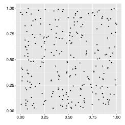
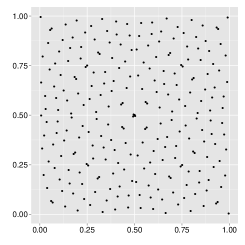
Figure 1: QMC versus Monte Carlo: $N=256$ points sampled independently and uniformly in $[0,1)^{2}$ (left); QMC sequence (Sobol’) in $[0,1)^{2}$ of the same length (right).

1.3 Introduction to RQMC

RQMC (randomized QMC) amounts to randomize the points $\mathbf{u}^{1:N}$ in such a way that (a) they still have low discrepancy (with probability one); and (b) each $\mathbf{u}^{n}\sim\mathcal{U}([0,1)^{d})$ marginally. The simplest construction of such RQMC point sets is the random shift method proposed by Cranley and Patterson, (1976) in which we take $\mathbf{u}^{n}=\mathbf{v}^{n}+\mathbf{w}\pmod{1}$, where $\mathbf{w}\sim\mathcal{U}([0,1)^{d})$ and $\mathbf{v}^{1:N}$ is a low-discrepancy point set.

RQMC has two advantages over QMC. First, one then obtains an unbiased estimator of the integral of interest:

$$\mathbb{E}\left\{\frac{1}{N}\sum_{n=1}^{N}\varphi(\mathbf{u}^{n})\right\}=\int_{[0,1)^{d}}\varphi(\mathbf{u})\,\mathrm{d}\mathbf{u},$$

which makes it possible to evaluate the approximation error through independent replications. We will see that, in our context, this unbiasedness property will also be very convenient for another reason: namely to provide an unbiased estimate of the likelihood of the considered state-space model.

Second, Owen, 1997a ; Owen, 1997b ; Owen, (1998) established that randomization may lead to better rates, in the following sense: under appropriate conditions, and for a certain type of randomization scheme known as nested scrambling, the mean square error of a RQMC estimator is $\mathcal{O}(N^{-3+\epsilon})$. The intuition behind this rather striking result is that randomization may lead to cancellation of certain error terms.

1.4 A note on array-RQMC

Consider the following problem: we have a Markov chain in $\mathcal{X}$, whose evolution may be formulated as

$$\mathbf{x}_{t}=\Gamma_{t}(\mathbf{x}_{t-1},\mathbf{u}_{t}),\quad\mathbf{u}_{t}\sim\mathcal{U}\left([0,1)^{d}\right),\quad t\geq 1,\quad\mathbf{x}_{0}\mbox{ is fixed},$$

and we wish to compute the expectation of $\sum_{t=1}^{T}\varphi_{t}(\mathbf{x}_{t})$, for certain functions $\varphi_{t}$.

From the two previous sections, we see that a simple approach to this problem would be to generate a QMC (or RQMC) point set $\mathbf{u}^{1:N}$ in $[0,1)^{dT}$, $\mathbf{u}^{n}=(\mathbf{u}_{1}^{n},\ldots,\mathbf{u}_{T}^{n})$, to transform $\mathbf{u}_{t}^{n}$ into $\mathbf{x}_{t}^{n}=\Gamma_{t}(\mathbf{x}_{t-1}^{n},\mathbf{u}_{t}^{n})$, and finally to return the corresponding empirical average, $N^{-1}\sum_{t=1}^{T}\varphi_{t}(\mathbf{x}_{t}^{n})$. The problem with this direct approach is that the dimension $dT$ of $\mathbf{u}^{1:N}$ may be very large, and, as we have seen, equidistribution properties of QMC point sets (as measured by the star discrepancy) deteriorate with the dimension.

An elegant alternative to this approach is the array-RQMC algorithm of L’Ecuyer et al., (2006), see also Lécot and Ogawa, (2002), Lécot and Tuffin, (2004), and L’Ecuyer et al., (2009). The main idea of this method is to replace the QMC point set in $[0,1)^{dT}$ by $T$ QMC points sets $\mathbf{u}_{t}^{1:N}$ in $[0,1)^{d}$. Then, $\mathbf{x}_{t}^{n}$ is obtained as $\mathbf{x}_{t}^{n}=\Gamma_{t}(\mathbf{x}_{t-1}^{a_{t-1}^{n}},\mathbf{u}_{t}^{n})$, where the ancestor $\mathbf{x}_{t-1}^{a_{t-1}^{n}}$ of $\mathbf{x}_{t}^{n}$ is chosen so as to be the $n$-th “smallest” point among the $\mathbf{x}_{t-1}^{n}$’s. Note that array-RQMC therefore requires to specify a total order for the state space $\mathcal{X}$; for instance one may define a certain $\omega:\mathcal{X}\rightarrow\mathbb{R}$ so that $\omega(\mathbf{x})\leq\omega(\mathbf{x}^{\prime})$ means that $\mathbf{x}$ is “smaller” than $\mathbf{x}^{\prime}$.

Array-RQMC is shown to have excellent empirical performance in the aforementioned papers. On the other hand, it is currently lacking in terms of supporting theory (see however l2008randomized, for $d=1$); in particular, it is not clear how to choose the order $\omega$, beside the obvious case where $\mathcal{X}\subset\mathbb{R}$. The SQMC algorithm we develop in this paper may be seen as an extension of array-RQMC to particle filtering. In particular, it re-uses the essential idea to generate one QMC point set at each step of the simulation process. As an added benefit, the convergence results we obtain for SQMC also apply to array-RQMC, provided the state space is ordered through the Hilbert curve, as explained later.

1.5 Background, plan and notations

QMC is already very popular in Finance for e.g. derivative pricing (Glasserman,, 2004), and one may wonder why it has not received more attention in Statistics so far. The main reason seems to be the perceived difficulty to adapt QMC to non-independent simulation such as MCMC (Markov chain Monte Carlo); see however Chen et al., (2011) and references therein, in particular Tribble, (2007), for exciting numerical and theoretical results in this direction which ought to change this perception.

Regarding SMC, we are aware of two previous attempts to develop QMC versions of these algorithms: Lemieux et al., (2001) and Fearnhead, (2005); see also Guo and Wang, (2006) who essentially proposed the same algorithm as Fearnhead, (2005). The first paper casts SMC as a Monte Carlo algorithm in $d(T+1)$ dimensions, where $d=\mathrm{dim}(\mathcal{X})$, and therefore requires to generate a low-discrepancy point set in $[0,1)^{d(T+1)}$. But, as we have already explained, such an approach may not work well when $d(T+1)$ is too large.

Our approach is closer to, and partly inspired by, the RPF (regularized particle filter) of Fearnhead, (2005), who, in the same spirit as array-RQMC, casts SMC as a sequence of $T+1$ successive importance sampling steps of dimension $d$. (The paper focus on the $d=1$ case.) The main limitation of the RPF is that it has complexity $\mathcal{O}(N^{2})$. This is because the importance sampling steps are defined with respect to a target which is a mixture of $N$ components, hence the evaluation of a single importance weight costs $\mathcal{O}(N)$.

The SQMC algorithm we develop in this paper has complexity $\mathcal{O}(N\log(N))$ per time step. It is also based on a sequence of $T+1$ importance sampling steps, but of dimension $d+1$; the first component is used to determine which ancestor $\mathbf{x}_{t-1}^{m}$ should be assigned to particle $\mathbf{x}_{t}^{n}$. For $d>1$, this requires us to “project” the set of ancestors $\mathbf{x}_{t-1}^{1:N}\in\mathcal{X}^{N}$ into $[0,1)^{N}$, by means of a space-filling curve known as the Hilbert curve. The choice of this particular space-filling curve is not only for computational convenience, but also because of its nice properties regarding conversion of discrepancy, as we will explain in the paper. (One referee pointed out to us that the use of Hilbert curve in the context of array-RQMC has been suggested by Wächter and Keller, (2008), but not implemented.)

The paper is organised as follows. Section 2 derives the general SQMC algorithm, first for $d=1$, then for any $d$ through the use of the Hilbert curve. Section 3 presents several convergence results; proofs of these results are in the Appendix. Section 4 shows how several standard extensions of SMC, such as forward smoothing, backward smoothing, and PMCMC, may be adapted to SQMC. Section 5 compares numerically SQMC with SMC. Section 6 concludes.

Most random variables in this work will be vectors in $\mathbb{R}^{d}$, and will be denoted in bold face, $\mathbf{u}$ or $\mathbf{x}$. In particular, $\mathcal{X}$ will be an open set of $\mathbb{R}^{d}$. The Lebesgue measure in dimension $d$ is denoted by $\lambda_{d}$. Let $\mathcal{P}(\mathcal{X})$ be the set of probability measures defined on $\mathcal{X}$ dominated by $\lambda_{d}$ (restricted to $\mathcal{X}$), and $\pi(\varphi)$ be the expectation of function $\varphi$ relative to $\pi\in\mathcal{P}(\mathcal{X})$. Let $a:b$ be the set of integers $\{a,\ldots,b\}$ for $a\leq b$. We also use this notation for collections of random variables, e.g. $\mathbf{x}_{t}^{1:N}=(\mathbf{x}_{t}^{1},\ldots,\mathbf{x}_{t}^{N})$, $\mathbf{x}_{0:t}=(\mathbf{x}_{0},\ldots,\mathbf{x}_{t})$ and so on.

2 SQMC

The objective of this section is to construct the SQMC algorithm. To this aim, we discuss how to rewrite SMC as a deterministic function of independent uniform variates $\mathbf{u}_{t}^{1:N}$, $t\in 0{:}T$, which then may be replaced by low-discrepancy point sets.

2.1 SMC formalisation

A closer inspection of our basic particle filter, Algorithm 1, reveals that this algorithm is entirely determined by (a) the sequence of proposal kernels $(m_{t})_{t\geq 0}$ (which determine how particles are simulated) and (b) the sequence of weight functions $(G_{t})_{t\geq 0}$ (which determine how particles are weighted). Our introduction to particle filtering focussed on the specific expression (1) for $G_{t}$, but useful SMC algorithms may be obtained by considering other weight functions; see e.g. the auxiliary particle filter of Pitt and Shephard, (1999), as explained in Johansen and Doucet, (2008), or the SMC algorithms for non-sequential problems mentioned in the introduction.

The exact expression and meaning of $m_{t}$ and $G_{t}$ will not play a particular role in the rest of the paper, so it is best to think of SMC from now on as a generic algorithm, again based on a certain sequence $(m_{t})$, $m_{0}(\mathrm{d}\mathbf{x}_{0})$ being an initial distribution, and $m_{t}(\mathbf{x}_{t-1},\mathrm{d}\mathbf{x}_{t})$ being a Markov kernel for $t\geq 1$, and a certain sequence of functions, $G_{0}:\mathcal{X}\rightarrow\mathbb{R}^{+}$, $G_{t}:\mathcal{X}\times\mathcal{X}\rightarrow\mathbb{R}^{+}$, which produces the following consistent (as $N\rightarrow+\infty$) estimators:

$$\frac{1}{N}\sum_{n=1}^{N}\varphi(\mathbf{x}_{t}^{n})\rightarrow\overline{\mathbb{Q}}_{t}(\varphi),\qquad\sum_{n=1}^{N}W_{t}^{n}\varphi(\mathbf{x}_{t}^{n})\rightarrow\mathbb{Q}_{t}(\varphi),$$

where $\varphi:\mathcal{X}\rightarrow\mathbb{R}$, and $\overline{\mathbb{Q}}_{t}$ and $\mathbb{Q}_{t}$ are defined as follows:

$$Z_{t} = \mathbb{E}\left[G_{0}(\mathbf{x}_{0})\prod_{s=1}^{t}G_{s}(\mathbf{x}_{s-1},\mathbf{x}_{s})\right],$$ (2)

$$\overline{\mathbb{Q}}_{t}(\varphi) = \frac{1}{Z_{t-1}}\mathbb{E}\left[\varphi(\mathbf{x}_{t})G_{0}(\mathbf{x}_{0})\prod_{s=1}^{t-1}G_{s}(\mathbf{x}_{s-1},\mathbf{x}_{s})\right],$$ (3)

$$\mathbb{Q}_{t}(\varphi) = \frac{1}{Z_{t}}\mathbb{E}\left[\varphi(\mathbf{x}_{t})G_{0}(\mathbf{x}_{0})\prod_{s=1}^{t}G_{s}(\mathbf{x}_{s-1},\mathbf{x}_{s})\right],$$ (4)

with expectations taken with respect to the law of the non-homogeneous Markov chain $(\mathbf{x}_{t})$, e.g.

$$Z_{t}=\int_{\mathcal{X}^{t+1}}\left\{G_{0}(\mathbf{x}_{0})\prod_{s=1}^{t}G_{s}(\mathbf{x}_{s-1},\mathbf{x}_{s})\right\}\,m_{0}(\mathrm{d}\mathbf{x}_{0})\prod_{s=1}^{t}m_{s}(\mathbf{x}_{s-1},\mathrm{d}\mathbf{x}_{s}),$$

and with the conventions that $Z_{-1}=1$ and empty products equal one; e.g. $\overline{\mathbb{Q}}_{0}(\varphi)=m_{0}(\varphi)$.

For instance, for the standard filtering problem covered in our introduction, where $G_{t}$ is set to (1), $\mathbb{Q}_{t}(\varphi)$ is the filtering expectation of $\varphi$, i.e. $\mathbb{E}[\varphi(\mathbf{x}_{t})|\mathbf{y}_{0:t}]$, and $\overline{\mathbb{Q}}_{t}(\varphi)$ is the predictive distribution of $\varphi$, i.e. $\mathbb{E}[\varphi(\mathbf{x}_{t})|\mathbf{y}_{0:t-1}]$.

2.2 Towards SQMC: SMC as a sequence of importance sampling steps

QMC requires to write any simulation as an explicit function of uniform variates. We therefore make the following assumption for our generic SMC sampler: to generate $\mathbf{x}_{0}^{n}\sim m_{0}(\mathrm{d}\mathbf{x}_{0})$, one computes $\mathbf{x}_{0}^{n}=\Gamma_{0}(\mathbf{u}_{0}^{n})$, and to generate $\mathbf{x}_{t}^{n}|\mathbf{x}_{t-1}^{n}\sim m_{t}(\mathbf{x}_{t-1},\mathrm{d}\mathbf{x}_{t})$, one computes $\mathbf{x}_{t}^{n}=\Gamma_{t}(\mathbf{x}_{t-1}^{n},\mathbf{u}_{t}^{n})$, where $\mathbf{u}_{t}^{n}\sim\mathcal{U}([0,1)^{d})$, and the functions $\Gamma_{t}$ are easy to evaluate.

Iteration $0$ of Algorithm 1 amounts to an importance sampling step, from $m_{0}(\mathrm{d}\mathbf{x}_{0})$ to $\mathbb{Q}_{0}(\mathrm{d}\mathbf{x}_{0})=m_{0}(\mathrm{d}\mathbf{x}_{0})G_{0}(\mathbf{x}_{0})/Z_{0}$, which produces the following estimator

$$\sum_{n=1}^{N}W_{0}^{n}\varphi(\mathbf{x}_{0}^{n})=\frac{\sum_{n=1}^{N}G_{0}(\mathbf{x}_{0}^{n})\varphi(\mathbf{x}_{0}^{n})}{\sum_{m=1}^{N}G_{0}(\mathbf{x}_{0}^{m})}$$

of $\mathbb{Q}_{0}(\varphi$). To introduce QMC at this stage, we take $\mathbf{x}_{0}^{n}=\Gamma_{0}(\mathbf{u}_{0}^{n})$ where $\mathbf{u}_{0}^{1:N}$ is a low-discrepancy point set in $[0,1)^{d}$.

The key remark that underpins SQMC is that iteration $t\geq 1$ of Algorithm 1 also amounts to an importance sampling step, but this time from

$$\overline{\mathbb{Q}}_{t}^{N}(\mathrm{d}(\widetilde{\mathbf{x}}_{t-1},\mathbf{x}_{t}))=\sum_{n=1}^{N}W_{t-1}^{n}\delta_{\mathbf{x}_{t-1}^{n}}(\mathrm{d}\widetilde{\mathbf{x}}_{t-1})m_{t}(\mathbf{x}_{t-1}^{n},\mathrm{d}\mathbf{x}_{t})$$ (5)

to

$$\mathbb{Q}_{t}^{N}(\mathrm{d}(\widetilde{\mathbf{x}}_{t-1},\mathbf{x}_{t}))=\frac{1}{\overline{\mathbb{Q}}_{t}^{N}(G_{t})}\overline{\mathbb{Q}}_{t}^{N}(\mathrm{d}(\widetilde{\mathbf{x}}_{t-1},\mathbf{x}_{t}))G_{t}(\widetilde{\mathbf{x}}_{t-1},\mathbf{x}_{t})$$

where $\mathbb{Q}_{t}^{N}$ and $\overline{\mathbb{Q}}_{t}^{N}$ are two random probability measures defined over $\mathcal{X}\times\mathcal{X}$, a set of dimension $2d$. In particular, the generation of random variables $a_{t-1}^{1:N}$ and $\mathbf{x}_{t}^{1:N}$ in Steps (a) and (b) of Algorithm 1 is equivalent to sampling $N$ times independently random variables $(\tilde{\mathbf{x}}_{t-1}^{n},\mathbf{x}_{t}^{n})$ from $\overline{\mathbb{Q}}_{t}^{N}(\mathrm{d}(\widetilde{\mathbf{x}}_{t-1},\mathbf{x}_{t}))$: i.e. $\tilde{\mathbf{x}}_{t-1}^{n}=\mathbf{x}_{t-1}^{a_{t-1}^{n}}$ (not to be mistaken with $\mathbf{x}_{t-1}^{n}$), and $\mathbf{x}_{t}^{n}\sim m_{t}(\tilde{\mathbf{x}}_{t-1}^{n},\mathrm{d}\mathbf{x}_{t})$.

Based on these remarks, the general idea behind SQMC is to replace at iteration $t$ the $N$ IID random numbers sampled from $\overline{\mathbb{Q}}_{t}^{N}(\mathrm{d}(\widetilde{\mathbf{x}}_{t-1},\mathbf{x}_{t}))$ by a low-discrepancy point set relative to the same distribution.

When $d=1$, this idea may be implemented as follows: generate a low-discrepancy point set $\mathbf{u}_{t}^{1:N}$ in $[0,1)^{2}$, let $\mathbf{u}_{t}^{n}=(u_{t}^{n},v_{t}^{n})$, then set $\tilde{\mathbf{x}}_{t-1}^{n}=\hat{F}_{N}^{-1}(u_{t}^{n})$, $\mathbf{x}_{t}^{n}=\Gamma_{t}(\tilde{\mathbf{x}}_{t-1}^{n},v_{t}^{n})$, where $\hat{F}_{N}^{-1}$ is the generalised inverse of the empirical CDF

$$\hat{F}_{N}(x)=\sum_{n=1}^{N}W_{t-1}^{n}\mathds{1}\left\{\mathbf{x}_{t-1}^{n}\leq x\right\},\quad x\in\mathcal{X}\subset\mathbb{R}.$$

It is easy to see that the most efficient way to compute $\tilde{\mathbf{x}}_{t-1}^{n}=\hat{F}_{N}^{-1}(u_{t}^{n})$ for all $n\in 1{:}N$ is (a) to sort the $\mathbf{x}_{t-1}^{n}$’s, i.e. to find permutation $\sigma$ such that $\mathbf{x}_{t-1}^{\sigma(1)}\leq\ldots\leq\mathbf{x}_{t-1}^{\sigma(N)}$, (b) to sort the $u_{t}^{1:N}$, call $\mathrm{sort}(u_{t}^{1:N})$ the corresponding result; (c) to obtain $a_{t-1}^{1:N}$ as the output of Algorithm 2, with inputs $\mathrm{sort}(u_{t}^{1:N})$ and $W_{t}^{\sigma(1:N)}$; and finally (d) set $\tilde{\mathbf{x}}_{t-1}^{n}=\mathbf{x}_{t-1}^{a_{t-1}^{n}}$.

Algorithm 3 gives a pseudo-code version of SQMC for any $d$, but note how Step (b) at times $t\geq 1$ simplifies to what we have just described for $d=1$.

When $d>1$, the inverse transform method cannot be used to sample from the marginal distribution of $\widetilde{\mathbf{x}}_{t-1}$ relative to $\overline{\mathbb{Q}}_{t}^{N}(\mathrm{d}(\widetilde{\mathbf{x}}_{t-1},\mathbf{x}_{t}))$, at least unless the $\mathbf{x}_{t-1}^{n}$ are “projected” to the real line in some sense. This is the point of the Hilbert curve presented in the next section.

2.3 The Hilbert space-filling curve

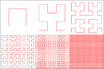
Figure 2: $H_{m}$ curve for $d=2$ and $m=1$ to $m=6$ (Source: Wikipedia)

The Hilbert curve is a continuous fractal map $H:[0,1]\rightarrow[0,1]^{d},$ which “fills” entirely $[0,1]^{d}$. $H$ is obtained as the limit of a sequence $(H_{m})$, $m\rightarrow+\infty$, the first terms of which are depicted in Figure 2.

The function $H$ admits a pseudo-inverse $h:[0,1]^{d}\rightarrow[0,1]$, i.e. $H\circ h(\mathbf{x})=\mathbf{x}$ for all $\mathbf{x}\in[0,1]^{d}$. $H$ is not a bijection because certain points $\mathbf{x}\in[0,1]^{d}$ have more than one pre-image through $H$; however the set of such points is of Lebesgue measure 0.

Informally, $H$ transforms $[0,1]$ into $[0,1]^{d}$, while preserving “locality”: if $x$, $x^{\prime}\in[0,1]$ are close, then $H(x)$ and $H(x^{\prime})$ are close as well. We will establish that $h$ also preserves discrepancy: a low-discrepancy point set in $[0,1)^{d}$ remains a low-discrepancy point set in $[0,1)$ when transformed through $h$. It is these properties that give to the Hilbert curve its appeal in the SQMC context (as opposed to other space filling curves, such as Z-ordering). We refer to Sagan, (1994), Butz, (1969) and Hamilton and Rau-Chaplin, (2008) for how to compute $h$ in practice for any $d\geq 2$. For $d=1$, we simply set $H(x)=h(x)=x$ for $x\in[0,1]$.

The following technical properties of $H$ and $H_{m}$ will be useful later (but may be skipped on first reading). For $m\geq 0$, let $\mathcal{I}_{m}^{d}=\left\{I_{m}^{d}(k)\right\}_{k=0}^{2^{md}-1}$ be the collection of consecutive closed intervals in $[0,1]$ of equal size $2^{-md}$ and such that $\cup\mathcal{I}_{m}^{d}=[0,1]$. For $k\geq 0$, $S_{m}^{d}(k)=H_{m}(I_{m}^{d}(k))$ belongs to $\mathcal{S}_{m}^{d}$, the set of the $2^{md}$ closed hypercubes of volume $2^{-md}$ that covers $[0,1]^{d}$, $\cup\mathcal{S}_{m}^{d}=[0,1]^{d}$; $S_{m}^{d}(k)$ and $S_{m}^{d}(k+1)$ are adjacent, i.e. have at least one edge in common (adjacency property). If we split $I_{m}^{d}(k)$ into the $2^{d}$ successive closed intervals $I_{m+1}^{d}(k_{i})$, $k_{i}=2^{d}k+i$ and $i\in 0:2^{d}-1$, then the $S_{m+1}^{d}(k_{i})$’s are simply the splitting of $S_{m}^{d}(k)$ into $2^{d}$ closed hypercubes of volume $2^{-d(m+1)}$ (nesting property). Finally, the limit $H$ of $H_{m}$ has the bi-measure property: $\lambda_{1}(A)=\lambda_{d}(H(A))$ for any measurable set $A\subset[0,1]$, and satisfies the Hölder condition $\|H(x_{1})-H(x_{2})\|_{\infty}\leq C_{H}|x_{1}-x_{2}|^{1/d}$ for any $x_{1},\,x_{2}\in[0,1]$.

2.4 SQMC for $d\geq 2$

Assume now $d\geq 2$, and consider the following change of variables at iteration $t\geq 1$:

$$h_{t-1}^{n}=h\circ\psi(\mathbf{x}_{t-1}^{n})\in[0,1]$$

where $h:[0,1]^{d}\rightarrow[0,1]$ is the inverse of the Hilbert curve defined in the previous section, and $\psi:\mathcal{X}\rightarrow[0,1]^{d}$ is some user-chosen bijection between $\mathcal{X}$ and $\psi(\mathcal{X})\subset[0,1]^{d}$. To preserve the low discrepancy property of $\mathbf{x}_{t-1}^{1:N}$ it is important to choose for $\psi$ a mapping which is discrepancy preserving. This requires to select $\psi$ such that $\psi(\mathbf{x})=\left(\psi_{1}(x_{1}),...,\psi_{d}(x_{d})\right)$ where the $\psi_{i}$’s are continuous and strictly monotone. But choosing such a $\psi$ is trivial in most applications; e.g. apply the logistic transformation component-wise when $\mathcal{X}=\mathbb{R}^{d}$ (see Section 5 for more details).

With this change of variables, we obtain particles $h_{t-1}^{1:N}$ that lie in $[0,1]$, and (5) becomes

$$\overline{\mathbb{Q}}_{t,h}^{N}\left(\mathrm{d}(\tilde{h}_{t-1},\mathbf{x}_{t})\right)=\sum_{n=1}^{N}W_{t-1}^{n}\delta_{h_{t-1}^{n}}(\mathrm{d}\tilde{h}_{t-1})m_{t}(\mathbf{x}_{t-1}^{n},\mathrm{d}\mathbf{x}_{t}).$$

Sampling a low-discrepancy sequence from $\overline{\mathbb{Q}}_{t,h}^{N}(\mathrm{d}\tilde{h}_{t-1},\mathrm{d}\mathbf{x}_{t})$ may then proceed exactly as for $d=1$; that is: use the inverse transform method to sample $N$ points $\tilde{h}_{t-1}^{1:N}$ from the marginal distribution $\overline{\mathbb{Q}}_{t,h}^{N}(\mathrm{d}\tilde{h}_{t-1})$, then sample $\mathbf{x}_{t}^{1:N}$ conditionally on $\tilde{\mathbf{x}}_{t-1}^{1:N}$, with $\tilde{\mathbf{x}}^{n}_{t-1}=\psi^{-1}\circ H(\tilde{h}_{t-1}^{n})$. The exact details of the corresponding operations are the same as for $d=1$. We therefore obtain the general SQMC algorithm as described in Algorithm 3.

At time $t=0$,

(a)

Generate a QMC or a RQMC point set $\mathbf{u}_{0}^{1:N}$ in $[0,1)^{d}$, and compute $\mathbf{x}_{0}^{n}=\Gamma_{0}(\mathbf{u}_{0}^{n})$ for each $n\in 1{:}N$.

(b)

Compute $w_{0}^{n}=G_{0}(\mathbf{x}_{0}^{n})$ and $W_{0}^{n}=w_{0}^{n}/\sum_{m=1}^{N}w_{0}^{m}$ for each $n\in 1{:}N$.

Iteratively, from time $t=1$ to time $t=T$,

(a)

Generate a QMC or a RQMC point set $\mathbf{u}_{t}^{1:N}$ in $[0,1)^{d+1}$; let $\mathbf{u}_{t}^{n}=(u_{t}^{n},\mathbf{v}_{t}^{n})\in[0,1)\times[0,1)^{d}$.

(b)

Hilbert sort: find permutation $\sigma_{t-1}$ such that $h\circ\psi(\mathbf{x}_{t-1}^{\sigma_{t-1}(1)})\leq\ldots\leq h\circ\psi(\mathbf{x}_{t-1}^{\sigma_{t-1}(N)})$ if $d\geq 2$, or $\mathbf{x}_{t-1}^{\sigma_{t-1}(1)}\leq\ldots\leq\mathbf{x}_{t-1}^{\sigma_{t-1}(N)}$ if $d=1$.

(c)

Find permutation $\tau$ such that $u_{t}^{\tau(1)}\leq...\leq u_{t}^{\tau(N)}$, generate $a_{t-1}^{1:N}$ using Algorithm 2, with inputs $u_{t}^{\tau(1:N)}$ and $W_{t-1}^{\sigma_{t-1}(1:N)}$, and compute $\mathbf{x}_{t}^{n}=\Gamma_{t}(\mathbf{x}_{t-1}^{\sigma_{t-1}(a_{t-1}^{n})},\mathbf{v}_{t}^{\tau(n)})$ for each $n\in 1{:}N$.

(e)

Compute $w_{t}^{n}=G_{t}(\mathbf{x}_{t-1}^{\sigma_{t-1}(a_{t-1}^{n})},\mathbf{x}_{t}^{n})$, and $W_{t}^{n}=w_{t}^{n}/\sum_{m=1}^{N}w_{t}^{m}$ for each $n\in 1{:}N$.

Algorithm 3 SQMC algorithm

To fully define SQMC, one must choose a particular method to generate point sets $\mathbf{u}_{t}^{1:N}$ at each iteration. If QMC point sets are generated, one obtains a deterministic algorithm, while if RQMC point sets are generated, one obtains a stochastic algorithm.

2.5 Complexity of SQMC

The complexity of both Steps (b) and (c) (for $t\geq 1$) of the SQMC algorithm is $\mathcal{O}(N\log N)$, because they include a sort operation. The complexity of Step (a) depends on the chosen method for generating the point sets $\mathbf{u}_{t}^{1:N}$. For instance, Hong and Hickernell, (2003) propose a $\mathcal{O}(N\log N)$ method that applies to most constructions of $(t,s)$-sequences (such as the Faure, the Sobol’, the Niederreiter or the Niederreiter-Xing sequences). The cost to randomize a QMC point set is only $\mathcal{O}(N)$ if one chooses the simple random shift approach, while nested scrambling methods for $(t,s)$-sequences, which are such that all the results below hold, may be implemented at cost $\mathcal{O}(N\log N)$ (Owen,, 1995; Hong and Hickernell,, 2003).

To summarise, the overall complexity of SQMC is $\mathcal{O}(N\log N)$, provided the method to generate the point sets $\mathbf{u}_{t}^{1:N}$ is chosen appropriately.

3 Convergence study

We concentrate on two types of asymptotic results (as $N\rightarrow+\infty$): consistency, and stochastic bounds, that is bounds on the mean square error for the randomized SQMC algorithm (i.e. SQMC based on randomized QMC point sets). We leave deterministic bounds of the error (for when deterministic QMC point sets are used) to future work. We find stochastic bounds more interesting, because (a) results from (Owen, 1997a, ; Owen, 1997b, ; Owen,, 1998) suggest one might obtain better convergence rates than for deterministic bounds; and (b) the randomized version of SQMC has more applications, as discussed in Section 4.

These results are specialised to the case where the simulation of $\mathbf{x}_{t}^{n}$ at time $t$ is based on the inverse transform method, as explained in Section 3.1. Certain of our results require $\mathcal{X}$ to be bounded, so for simplicity we take $\mathcal{X}=[0,1)^{d}$, and $\psi$ is set to the identity function. (Recall that, to deal with certain QMC technicalities, we follow the standard practice of taking $\mathcal{X}=[0,1)^{d}$ rather than $\mathcal{X}=[0,1]^{d}$.) The fact that $\mathcal{X}$ is bounded may not be such a strong restriction, as our results allow for unbounded test functions $\varphi$; thus, one may accommodate for an unbounded state space (and expectations with respect to that space) through appropriate variable transforms.

We introduce the following extreme norm. For any signed measure $\mu$ over $\mathcal{X}=[0,1)^{d}$,

$$\|\mu\|_{\mathrm{E}}=\sup_{B\in\mathcal{B}_{[0,1)^{d}}}\left|\mu(B)\right|,\quad\mathcal{B}_{[0,1)^{d}}=\left\{B:\>B=\prod_{i=1}^{d}[a_{i},b_{i}]\subset[0,1)^{d},\>a_{i}<b_{i}\right\}$$

which generalises the extreme discrepancy in the following sense:

$$\|\mathcal{S}(\mathbf{x}^{1:N})-\lambda_{d}\|_{\mathrm{E}}=D(\mathbf{x}^{1:N})$$

for any point set $\mathbf{x}^{1:N}$ in $\mathcal{X}$, where $\mathcal{S}$ is the operator that associates to $\mathbf{x}^{1:N}$ its empirical distribution:

$$\mathbf{x}^{1:N}\in\mathcal{X}^{N}\mapsto\mathcal{S}(\mathbf{x}^{1:N})=\frac{1}{N}\sum_{n=1}^{N}\delta_{\mathbf{x}^{n}}.$$

Our consistency results will be stated with this norm. Note that $\|\pi^{N}-\pi\|_{\mathrm{E}}\rightarrow 0$ implies $\left|\pi^{N}(\varphi)-\pi(\varphi)\right|\rightarrow 0$ for any continuous, bounded function $\varphi$, by portmanteau lemma (Van der Vaart,, 2007, Lemma 2.2).

The next subsection explains how the inverse method may be used to generate $\mathbf{x}_{t}^{n}$ given $\mathbf{x}_{t-1}^{n}$. The two following subsections state preliminary results that should provide insights on the main ideas that underpin the proofs of our convergence results. Readers interested mostly in the main results may skip these subsections and go directly to Section 3.4 (consistency) and Section 3.5 (stochastic bounds).

This section will use the following standard notations: $\|\varphi\|_{\infty}$ for the supremum norm for functions $\varphi$, $L_{2}(\mathcal{X},\mu)$ for the set of square integrable functions $\varphi:\mathcal{X}\rightarrow\mathbb{R}$ and $\mathcal{C}_{b}(\mathcal{X})$ for the set of continuous, bounded functions $\varphi:\mathcal{X}\rightarrow\mathbb{R}$.

3.1 Inverse transform method

We discuss here how to write the simulation of $\mathbf{x}_{t}^{n}$ as $\mathbf{x}_{t}^{n}=\Gamma_{t}(\mathbf{x}_{t-1}^{n},\mathbf{u}_{t}^{n})$, using the inverse transform method. Our convergence results are specialised to this particular $\Gamma_{t}$.

For a generic distribution $\pi\in\mathcal{P}(\mathcal{X})$, $\mathcal{X}\subset\mathbb{R}^{d}$, let $F_{\pi}$ be the Rosenblatt transformation (Rosenblatt,, 1952) of $\pi$ defined through the following chain rule decomposition:

$$F_{\pi}(\mathbf{x})=\left(u_{1},\ldots,u_{d}\right)^{T},\quad\mathbf{x}=(x_{1},\ldots,x_{d})^{T}\in\mathcal{X},$$

where, recursively, $u_{1}=F_{\pi,1}(x_{1}),$ $F_{\pi,1}$ being the CDF of the marginal distribution of the first component (relative to $\pi$), and for $i\geq 2$, $u_{i}=F_{\pi,i}(x_{i}|x_{1:i-1})$, $F_{\pi,i}(\cdot|x_{1:i-1})$ being the CDF of component $x_{i}$, conditional on $(x_{1},\ldots,x_{i-1}$), again relative to $\pi$. Similarly, we define the multivariate GICDF (generalised inverse CDF) $F_{\pi}^{-1}$ through the following chain rule decomposition:

$$F_{\pi}^{-1}(\mathbf{u})=\left(x_{1},\ldots,x_{d}\right)^{T},\quad\mathbf{u}=(u_{1},\ldots,u_{d})^{T}\in[0,1)^{d},$$

where, recursively, $x_{1}=F_{\pi,1}^{-1}(u_{1}),$ $F_{\pi,1}^{-1}$ being the GICDF of the marginal distribution of the first component (relative to $\pi$), and for $i\geq 2$, $x_{i}=F_{\pi,i}^{-1}(u_{i}|x_{1:i-1})$, $F_{\pi,i}^{-1}(\cdot|x_{1:i-1})$ being the GICDF of component $x_{i}$, conditional on $(x_{1},\ldots,x_{i-1}$), again relative to $\pi$. Note that this function depends on the particular order of the components of $\pi$. For some probability kernel $K:\mathcal{X}\rightarrow\mathcal{P}(\mathcal{X})$, define similarly $F_{K}(\mathbf{x},\cdot)$ and $F_{K}^{-1}(\mathbf{x},\cdot)$ as, respectively, the Rosenblatt transformation and the multivariate GICDF of distribution $K(\mathbf{x},\mathrm{d}\mathbf{x}^{\prime})$ for a fixed $\mathbf{x}$.

It is well known that taking $\Gamma_{0}=F_{m_{0}}^{-1}$, and $\Gamma_{t}=F_{m_{t}}^{-1}$ lead to valid simulations algorithms, i.e. if $\mathbf{x}_{0}^{n}=F_{m_{0}}^{-1}(\mathbf{u}_{0}^{n})$, resp. $\mathbf{x}_{t}^{n}=F_{m_{t}}^{-1}(\mathbf{x}_{t-1},\mathbf{u}_{t}^{n})$, then $\mathbf{x}_{0}^{n}\sim m_{0}(\mathrm{d}\mathbf{x}_{0})$, resp. $\mathbf{x}_{t}^{n}|\mathbf{x}_{t-1}^{n}\sim m_{t}(\mathbf{x}_{t-1}^{n},\mathrm{d}\mathbf{x}_{t})$.

3.2 Preliminary results: importance sampling

Since SQMC is based on importance sampling (e.g. Iteration $0$ of Algorithm 3), we need to establish the validity of importance sampling based on low-discrepancy point sets; see Götz, (2002); Aistleitner and Dick, (2014) for other results on QMC-based importance sampling.

Theorem 1.

Let $\pi$ and $q$ be two probability measures on $[0,1)^{d}$ such that the Radon-Nikodym derivative $w(\mathbf{x})=\pi(\mathrm{d}\mathbf{x})/q(\mathrm{d}\mathbf{x})$ is continuous and bounded. Let $(\mathbf{x}^{1:N})$ be a sequence of point sets in $[0,1)^{d}$ such that $\|\mathcal{S}(\mathbf{x}^{1:N})-q\|_{\mathrm{E}}\rightarrow 0$ as $N\rightarrow+\infty$, and define

$$\pi^{N}=\sum_{n=1}^{N}W^{n}\delta_{\mathbf{x}^{n}},\quad W^{n}=\frac{w(\mathbf{x}^{n})}{\sum_{m=1}^{N}w(\mathbf{x}^{m})}.$$

Then, $\|\pi^{N}-\pi\|_{\mathrm{E}}\rightarrow 0$ as $N\rightarrow+\infty$.

See Section A.1.2 of the Appendix for a proof.

Recall that in our notations we drop the dependence of point sets on $N$, i.e. we write $(\mathbf{x}^{1:N})$ rather than $(\mathbf{x}^{N,1:N})$, although in full generality $\mathbf{x}^{1:N}$ may not necessarily be the $N$ first points of a fixed sequence.

The next theorem gives the stochastic error rate when a RQMC point set is used.

Theorem 2.

Consider the set-up of Theorem 1. Let $(\mathbf{u}^{1:N})$ be a sequence of random point sets in $[0,1)^{d}$ such that $\mathbf{u}^{n}\sim\mathcal{U}([0,1)^{d})$ marginally and, $\forall\varphi\in L_{2}([0,1)^{d},\lambda_{d})$,

$$\mathrm{Var}\left(\frac{1}{N}\sum_{n=1}^{N}\varphi(\mathbf{u}^{n})\right)={\scriptscriptstyle\mathcal{O}}\Big{(}r(N)\Big{)},$$

where $r(N)\rightarrow 0$ as $N\rightarrow+\infty$. Let $\mathbf{x}^{1:N}=F_{q}^{-1}(\mathbf{u}^{1:N})$ and assume that either one of the following two conditions is verified:

1. $F_{q}^{-1}$ is continuous and, for any $\epsilon>0$, there exists a $N_{\epsilon}\in\mathbb{N}$ such that, almost surely, $D^{\star}(\mathbf{u}^{1:N})\leq\epsilon$, $\forall N\geq N_{\epsilon}$;

2. for any $\epsilon>0$ there exists a $N_{\epsilon}\in\mathbb{N}$ such that, almost surely,

   $$\|\mathcal{S}(\mathbf{x}^{1:N})-q\|_{\mathrm{E}}\leq\epsilon,\quad\forall N\geq N_{\epsilon}.$$

Then, for all $\varphi\in L_{2}(\mathcal{X},\pi)$,

$$\mathbb{E}\left|\pi^{N}(\varphi)-\pi(\varphi)\right|={\scriptscriptstyle\mathcal{O}}\Big{(}r(N)^{1/2}\Big{)},\quad\mathrm{Var}\left(\pi^{N}(\varphi)\right)={\scriptscriptstyle\mathcal{O}}\Big{(}r(N)\Big{)}.$$

See Section A.1.2 of the Appendix for a proof.

To fix ideas, note that several RQMC strategies reach the Monte Carlo error rate and therefore fulfil the assumptions above with $r(N)=N^{-1+\epsilon}$ for any $\epsilon>0$ (see e.g. Owen, 1997a, ; Owen,, 1998). In addition, nested scrambling methods for $(t,s)$-sequences in base $b$ (Owen,, 1995; Matoǔsek,, 1998; Hong and Hickernell,, 2003) are such that $r(N)=N^{-1}$. This result is established for $N=\lambda b^{m}$ in Owen, 1997a ; Owen, (1998) and extended for an arbitrary $N$ in Gerber, (2014).

3.3 Preliminary results: Hilbert curve and discrepancy

We motivated the use of the Hilbert curve as a way to transform back and forth between $[0,1]^{d}$ and $[0,1]$ while preserving low discrepancy in some sense. This section formalises this idea.

For a probability measure $\pi$ on $[0,1)^{d}$, we write $\pi_{h}$ the image by $h$ of $\pi$. For a kernel $K:[0,1)^{d}\rightarrow\mathcal{P}(\mathcal{X})$, we write $\pi_{h}\otimes K_{h}\left(\mathrm{d}(h_{1},\mathbf{x}_{2})\right)$ the image of $\pi\otimes K$ by the mapping $(\mathbf{x}_{1},\mathbf{x}_{2})\in[0,1)^{d}\times\mathcal{X}\mapsto(h(\mathbf{x}_{1}),\mathbf{x}_{2})$, where $\pi\otimes K$ denotes the joint probability measure $\pi(\mathrm{d}\mathbf{x}_{1})K(\mathbf{x}_{1},\mathrm{d}\mathbf{x}_{2})$.

The following theorem is a technical result on the conversion of discrepancy through $h$.

Theorem 3.

Let $(\pi^{N})$ be a sequence of probability measure on $[0,1)^{d}$ such that, $\|\pi^{N}-\pi\|_{\mathrm{E}}\rightarrow 0$, where $\pi(\mathrm{d}\mathbf{x})=\pi(\mathbf{x})\lambda_{d}(\mathrm{d}\mathbf{x})$ admits a bounded probability density $\pi(\mathbf{x})$. Then

$$\|\pi_{h}^{N}-\pi_{h}\|_{\mathrm{E}}\rightarrow 0,\quad\mbox{as }N\rightarrow+\infty.$$

See Section A.2.1 of the Appendix for a proof.

The following theorem is an extension of Hlawka and Mück, (1972, “Satz 2”), which establishes the validity, in the context of QMC, of the multivariate GICDF approach described in Section 3.1. More precisely, for a probability measure $\pi$ on $[0,1)^{d}$, Hlawka and Mück, (1972, “Satz 2”) show that $\|\mathcal{S}\left(F^{-1}_{\pi}(\mathbf{u}^{1:N})\right)-\pi\|_{\mathrm{E}}\leq cD^{\star}(\mathbf{u}^{1:N})^{1/d}$ (under some conditions on $F_{\pi}$, see below).

Theorem 4.

Let $K:[0,1)^{d_{1}}\rightarrow\mathcal{P}\left([0,1)^{d_{2}}\right)$ be a Markov kernel and assume that:

1. For a fixed $\mathbf{x}_{1}\in[0,1)^{d_{1}}$, the $i$-th coordinate of $F_{K}\left(\mathbf{x}_{1},\mathbf{x}_{2}\right)$ is strictly increasing in $x_{2i}\in[0,1)$, $i\in 1:d_{2}$, and, viewed as a function of $\mathbf{x}_{1}$ and $\mathbf{x}_{2}$, $F_{K}\left(\mathbf{x}_{1},\mathbf{x}_{2}\right)$ is Lipschitz;

2. $\pi^{N}(\mathrm{d}\mathbf{x})=\sum_{n=1}^{N}W_{N}^{n}\delta_{\mathbf{x}_{1}^{n}}(\mathrm{d}\mathbf{x})$, $\mathbf{x}_{1}^{n}\neq\mathbf{x}_{1}^{m}$ $\forall n\neq m\in 1:N$, and $\max_{n\in 1:N}W_{N}^{n}\rightarrow 0$.

3. The sequence $(\pi^{N})$ is such that $\|\pi^{N}-\pi\|_{\mathrm{E}}\rightarrow 0$ as $N\rightarrow+\infty$, where $\pi(\mathrm{d}\mathbf{x})=\pi(\mathbf{x})\lambda_{d_{1}}(\mathrm{d}\mathbf{x})$ admits a strictly positive bounded density $\pi$.

Let $(\mathbf{u}^{1:N})$, $\mathbf{u}^{n}=(u^{n},\mathbf{v}^{n})\in[0,1)^{1+d_{2}}$, be a sequence of point sets in $[0,1)^{1+d_{2}}$ such that $D^{\star}(\mathbf{u}^{1:N})\rightarrow 0$ as $N\rightarrow+\infty$, and define $P_{h}^{N}=\left(h^{1:N},\mathbf{x}_{2}^{1:N}\right)$ where

$$h^{n}=F_{\pi_{h}^{N}}^{-1}(u^{n}),\quad\tilde{\mathbf{x}}_{1}^{n}=H(h^{n}),\quad\mathbf{x}_{2}^{n}=F_{K}^{-1}\left(\tilde{\mathbf{x}}_{1}^{n},\mathbf{v}^{n}\right).$$

Then

$$\|\mathcal{S}(P_{h}^{N})-\pi_{h}^{N}\otimes K_{h}\|_{\mathrm{E}}\rightarrow 0,\quad\mbox{as }N\rightarrow+\infty.$$

See Section A.2.2 of the Appendix for a proof.

Assumption 1 regarding the regularity of the vector-valued function $F_{K}$ is the main assumption of the above theorem and comes from Hlawka and Mück, (1972, “Satz 2”). It is verified as soon as kernel $K$ admits a density that is continuously differentiable on $[0,1)^{d}$ (Hlawka and Mück,, 1972, p.232). Assumption 2 is a technical condition, which will always hold under the assumptions of our main results.

3.4 Consistency

We are now able to establish the consistency of SQMC; see Appendix A.3 for a proof of the following theorem. For convenience, let $F_{m_{t}}(\mathbf{x}_{t-1},\mathbf{x}_{t})=F_{m_{0}}(\mathbf{x}_{0})$ when $t=0$.

Theorem 5.

Consider the set-up of Algorithm 3 where, for all $t\in 0:T$, $(\mathbf{u}_{t}^{1:N})$ is a (non random) sequence of point sets in $[0,1)^{d_{t}}$, with $d_{0}=d$ and $d_{t}=d+1$ for $t>0$, such that $D^{\star}(\mathbf{u}_{t}^{1:N})\rightarrow 0$ as $N\rightarrow+\infty$. Assume the following holds for all $t\in 0{:}T$:

1. The components of $\mathbf{x}_{t}^{1:N}$ are pairwise distinct, $\mathbf{x}_{t}^{n}\neq\mathbf{x}_{t}^{m}$ for $n\neq m$.

2. $G_{t}$ is continuous and bounded;

3. $F_{m_{t}}(\mathbf{x}_{t-1},\mathbf{x}_{t})$ verifies Assumption 1 of Theorem 4 ;

4. $\mathbb{Q}_{t}(\mathrm{d}\mathbf{x}_{t})=p_{t}(\mathbf{x}_{t})\lambda_{d}(\mathrm{d}\mathbf{x}_{t})$ where $p_{t}(\mathbf{x}_{t})$ is a strictly positive bounded density.

Let $\widehat{\mathbb{Q}}_{t}^{N}(\mathrm{d}\mathbf{x}_{t})=\sum_{n=1}^{N}W_{t}^{n}\delta_{\mathbf{x}_{t}^{n}}(\mathrm{d}\mathbf{x}_{t})$. Then, under Assumptions 1-4, as $N\rightarrow+\infty$,

$$\|\widehat{\mathbb{Q}}_{t}^{N}-\mathbb{Q}_{t}\|_{\mathrm{E}}\rightarrow 0,\quad\forall t\in 0{:}T.$$

Assumption 1 is stronger than necessary because for the result to hold it is enough that the number of identical particles does not grow too quickly as $N\rightarrow+\infty$. Note that this is a very weak restriction since Assumption 1 holds almost surely when RQMC point sets are used, since then the particles are generated from a continuous GICDF. The assumption that the weight functions $(G_{t})$ are bounded is standard in SMC literature (see e.g. Del Moral,, 2004).

3.5 Stochastic bounds

Our second main result concerns stochastic bounds for the randomized version of SQMC, i.e. SQMC based on randomized point sets $(\mathbf{u}_{t}^{n})$. See Section A.4 of the Appendix for a proof of the next result.

Theorem 6.

Consider the set-up of Algorithm 3 where $(\mathbf{u}_{t}^{1:N})$, $t\in 0:T$, are independent sequences of random point sets in $[0,1)^{d_{t}}$, with $d_{0}=d$ and $d_{t}=d+1$ for $t>0$, such that, for all $t\in 0:T$, $\mathbf{u}_{t}^{n}\sim\mathcal{U}([0,1)^{d_{t}})$ marginally and

1. For any $\epsilon>0$, there exists a $N_{\epsilon,t}>0$ such that, almost surely, $D^{\star}(\mathbf{u}_{t}^{1:N})\leq\epsilon$, $\forall N\geq N_{\epsilon,t}$.

2. For any function $\varphi\in L_{2}\left([0,1)^{d_{t}},\lambda_{d_{t}}\right)$, $\mathrm{Var}\left(\frac{1}{N}\sum_{n=1}^{N}\varphi(\mathbf{u}_{t}^{n})\right)\leq C^{*}\,\sigma_{\varphi}^{2}r(N)$ where $\sigma_{\varphi}^{2}=\int\left\{\varphi(\mathbf{u})-\int\varphi(\mathbf{v})\mathrm{d}\mathbf{v}\right\}^{2}\mathrm{d}\mathbf{u}$, and where both $C^{*}$ and $r(N)$ do not depend on $\varphi$.

In addition, assume that the Assumptions of Theorem 5 are verified and that $F_{m_{0}}^{-1}$ is continuous. Let $\varphi\in L_{2}([0,1)^{d},\mathbb{Q}_{t})$ for all $t\in 0{:}T$. Then, $\forall t\in 0{:}T$,

$$\mathbb{E}\left|\widehat{\mathbb{Q}}_{t}^{N}(\varphi)-\mathbb{Q}_{t}(\varphi)\right|=\mathcal{O}\Big{(}r(N)^{1/2}\Big{)},\quad\mathrm{Var}\Big{(}\widehat{\mathbb{Q}}_{t}^{N}(\varphi)\Big{)}=\mathcal{O}\Big{(}r(N)\Big{)}.$$

Note that the implicit constants in the line above may depend on $\varphi$. Assumptions 1 and 2 are verified for $r(N)=N^{-1}$ if $\mathbf{u}_{t}^{1:N}$ is the first $N$ points of a nested scrambled $(t,s)$-sequences in base $b\geq 2$. This result is established for $N=\lambda b^{m}$ in Owen, 1997a ; Owen, (1998) and can be extended to any pattern of $N$ using Hickernell and Yue, (2001, Lemma 1). Consequently, for this construction of RQMC point sets, Theorem 6 shows that the approximation error of SQMC goes to zero at least as fast as for SMC. However, contrary to the $\mathcal{O}(N^{-1})$ convergence rate of SMC, this rate for SQMC based on nested scrambled $(t,s)$-sequences is not exact but results from a worst case analysis. We can therefore expect to reach faster convergence on a smaller class of functions. The following result shows that it is indeed the case on the class on continuous and bounded functions; see Section A.4.4 of the Appendix for a proof.

Theorem 7.

Consider the set-up of Algorithm 3 where $(\mathbf{u}_{t}^{1:N})$, $t\in 0{:}T$, are $(t,d_{t})$-sequences in base $b\geq 2$, with $d_{0}=d$ and $d_{t}=d+1$ for $t>0$, independently scrambled such that results in Owen, 1997a ; Owen, (1998) hold. Let $N=\lambda b^{m}$, $1\leq\lambda<b$, and assume the following holds:

1. Assumptions of Theorem (6) are verified;

2. For $t\in 1{:}T$, $F^{-1}_{m_{t}}(\mathbf{x}_{t-1},\mathbf{x}_{t})$ is a continuous function of $\mathbf{x}_{t-1}$.

Let $\varphi\in\mathcal{C}_{b}(\mathcal{X})$. Then, $\forall t\in 0{:}T$,

$$\mathbb{E}|\widehat{\mathbb{Q}}_{t}^{N}(\varphi)-\mathbb{Q}_{t}(\varphi)|={\scriptscriptstyle\mathcal{O}}(N^{-1/2}),\quad\mathrm{Var}(\widehat{\mathbb{Q}}_{t}^{N}(\varphi))={\scriptscriptstyle\mathcal{O}}(N^{-1}).$$

Thus, for SQMC based on the first $N=\lambda b^{m}$ points of nested scrambled $(t,s)$-sequences in base $b$, one obtains that the stochastic error of (the random version of) SQMC converges faster than for SMC. Note that we can relax the constraint on $N$ in Theorem 7 using Gerber, (2014, Corollary 2).

4 Extensions

4.1 Unbiased estimation of evidence, PMCMC

Like SMC, the randomized version of SQMC (that is SQMC based on RQMC point sets) provides an unbiased estimator of the normalising constant $Z_{t}$ of the Feynman-Kac model, see (2).

Lemma 8.

Provided that $\mathbf{u}_{t}^{1:N}$ is a RQMC point set in $[0,1)^{d_{t}}$ for $t\in 0:T$ (i.e. $\mathbf{u}_{t}^{n}\sim\mathcal{U}([0,1)^{d_{t}})$ marginally), with $d_{0}=d$ and $d_{t}=d+1$ for $t>0$, the following quantity

$$Z_{t}^{N}=\left\{\frac{1}{N}\sum_{n=1}^{N}G_{0}(\mathbf{x}_{0}^{n})\right\}\prod_{s=1}^{t}\left\{\frac{1}{N}\sum_{n=1}^{N}G_{s}(\mathbf{x}_{s-1}^{a_{s-1}^{n}},\mathbf{x}_{s}^{n})\right\}$$

is an unbiased estimator of $Z_{t}$, $\mathbb{E}[Z_{t}^{N}]=Z_{t}$.

We omit the proof, as it follows the same steps as for SMC (Del Moral,, 1996).

In a state-space model parametrised by $\theta\in\Theta$, $Z_{t}=Z_{t}(\theta)$ is the marginal likelihood of the data up to time $t$. One may want to implement a Metropolis-Hastings sampler with respect to posterior density $\pi_{T}(\theta)\propto p(\theta)Z_{T}(\theta)$ for the full dataset and for a prior distribution $p(\theta)$, but $Z_{T}(\theta)$ is typically intractable.

Andrieu et al., (2010) established that, by substituting $Z_{T}(\theta)$ with an unbiased estimate of $Z_{T}(\theta)$ in a Metropolis sampler, one obtains an exact MCMC (Markov chain Monte Carlo) algorithm, in the sense that the corresponding MCMC kernel leaves invariant $\pi_{T}(\theta)$. The so obtained algorithm is called PMMH (Particle marginal Metropolis-Hastings). Andrieu et al., (2010) use SMC to obtain an unbiased estimate of $Z_{T}(\theta$), that is, at each iteration a SMC sampler is run to obtain that estimate. We will call PMMH-SQMC the same algorithm, but with SQMC replacing SMC for the evaluation of an unbiased estimate of the likelihood.

The acceptance rate of PMMH depends directly on the variability of the estimates of $Z_{T}(\theta)$. Since the point of (randomized) SQMC is to provide estimates with a lower variance than SMC (for a given $N$), one may expect that PMMH-SQMC may require a smaller number of particles than standard PMMH for satisfactory acceptance rates; see Section 5 for a numerical illustration of this.

4.2 Smoothing

Smoothing amounts to compute expectations $\mathbb{Q}_{t}(\varphi)$ of functions $\varphi$ of the complete trajectory $\mathbf{x}_{0:t}$; e.g. $\mathbb{Q}_{t}(\varphi)$ is the expectation of $\varphi(\mathbf{x}_{0:t})$ conditional on data $\mathbf{y}_{0:t}$ for a state-space model with Markov process $\left(\mathbf{x}_{t}\right)$ and observed process $\left(\mathbf{y}_{t}\right)$. See Briers et al., (2010) for a general overview on SMC smoothing algorithms. This section discusses how to adapt certain of these algorithms to SQMC.

4.2.1 Forward smoothing

Forward smoothing amounts to carry forward the complete trajectories of the particles, rather than simply keeping the last component $\mathbf{x}_{t}^{n}$ (as in Algorithm 1). A simple way to formalise forward smoothing is to introduce a path Feynman-Kac  model, corresponding to the inhomogeneous Markov process $\mathbf{z}_{t}=\mathbf{x}_{0:t}$, and weight function (abusing notations) $G_{t}(\mathbf{z}_{t})=G_{t}(\mathbf{x}_{t})$. Then forward smoothing amounts to Algorithm 1 applied to this path Feynman-Kac  model (substituting $\mathbf{x}_{t}$ with $\mathbf{z}_{t}=\mathbf{x}_{0:t}$).

One may use the same remark to define a SQMC version of forward smoothing: i.e. simply apply SQMC to the same path Feynman-Kac  model. The only required modification is that the Hilbert sort of Step (b) at times $t\geq 1$ must now operate on some transformation of the vectors $\mathbf{z}_{t}^{n}$, of dimension $(t+1)d$, rather than vectors $\mathbf{x}_{t}^{n}$ of dimension $d$ as in the original version.

Forward smoothing is sometimes used to approximate the smoothing expectation of additive functions, $\varphi(\mathbf{x}_{0:t})=\sum_{s=0}^{t}\tilde{\varphi}(\mathbf{x}_{s})$, such as the score function of certain models (e.g. Poyiadjis et al.,, 2011). In that case, one may instead apply SQMC to the Feynman-Kac  model corresponding to the inhomogeneous Markov process $\mathbf{z}_{t}=(\sum_{s=0}^{t-1}\tilde{\varphi}(\mathbf{x}_{s}),\mathbf{x}_{t})$. This means that in practice, one may implement the Hilbert sort on a space of much lower dimension (i.e. the dimension of this new $\mathbf{z}_{t}$), which is computationally more convenient.

4.2.2 Backward smoothing

Backward smoothing consists of two steps: (a) a forward pass, where SMC is run from time $0$ to time $T$; and (b) a backward pass, where one constructs a trajectory $\tilde{\mathbf{x}}_{0:T}$ recursively backwards in time, by selecting randomly each component $\tilde{\mathbf{x}}_{t}$ out of the $N$ particle values $\mathbf{x}_{t}^{n}$ generated during the forward pass. An advantage of backward smoothing is that it is less prone to degenerate than forward smoothing. A drawback of backward smoothing is that generating a single trajectory costs $\mathcal{O}(N)$, hence obtaining $N$ of them costs $\mathcal{O}(N^{2}$).

Backward smoothing for SQMC may be implemented in a similar way to SMC: see Algorithm 4 for the backward pass that generates $N_{B}$ trajectories $\tilde{\mathbf{x}}^{1:N_{B}}_{0:T}$ from the output of the SQMC algorithm. Note that backward smoothing requires that the Markov kernel $m_{t}(\mathbf{x}_{t-1},\mathrm{d}\mathbf{x}_{t})$ admits a closed-form density $m_{t}(\mathbf{x}_{t}|\mathbf{x}_{t-1})$ with respect to an appropriate dominating measure. Then one may compute empirical averages over the so obtained $N_{B}$ trajectories to obtain smoothing estimates in the usual way.

Algorithm 4 Backward step of SQMC backward smoothing

$\mathbf{x}_{0:T}^{\sigma_{t}(1:N)}$, $W_{0:T}^{\sigma_{t}(1:N)}$ (output of SQMC obtained after the Hilbert sort step, i.e for all $t\in 0{:}T$, $h\circ\psi(\mathbf{x}_{t}^{\sigma_{t}(n)})\leq h\circ\psi(\mathbf{x}_{t}^{\sigma_{t}(m)})$, $n\leq m$) and $\tilde{\mathbf{u}}^{1:N_{B}}$ a point set in $[0,1)^{T+1}$; let $\tilde{\mathbf{u}}^{n}=(\tilde{u}_{0}^{n},\dots,\tilde{u}_{T}^{n})$.

$\tilde{\mathbf{x}}^{1:N_{B}}_{0:T}$ ($N_{B}$ trajectories in $\mathcal{X}^{T+1}$)

Find permutation $\tau$ such that $\tilde{u}_{0}^{\tau(1)}\leq...\leq\tilde{u}_{0}^{\tau(N_{B})}$, generate $\tilde{a}_{T}^{1:N_{B}}$ using Algorithm 2, with inputs $\tilde{u}_{0}^{\tau(1:N_{B})}$ and $W_{T}^{\sigma_{T}(1:N)}$, and set $\tilde{\mathbf{x}}_{T}^{n}=\mathbf{x}_{T}^{\tilde{a}_{T}^{n}}$ for all $n\in 1{:}N_{B}$.

for $t=T-1\rightarrow 0$ do

     For $n\in 1{:}N_{B}$, set $\tilde{\mathbf{x}}_{t}^{n}=\mathbf{x}_{t}^{\tilde{a}_{t}^{n}}$ where $\tilde{a}_{t}^{n}=F_{\pi^{n}_{t}}^{-1}(\tilde{u}_{T-t}^{\tau(n)})$, $\pi_{t}^{n}=\sum_{m=1}^{N}\widetilde{W}^{m}_{t}(\tilde{\mathbf{x}}^{n}_{t+1})\delta_{m}$ and, for $m\in 1{:}N$,

$$\widetilde{W}_{t}^{m}(\mathbf{x}_{t+1})=W_{t}^{\sigma_{t}(m)}m_{t}(\mathbf{x}_{t+1}|\mathbf{x}_{t}^{\sigma_{t}(m)})/\left\{\sum_{n=1}^{N}W_{t}^{n}m_{t}(\mathbf{x}_{t+1}|\mathbf{x}_{t}^{n})\right\}.$$

end for

5 Numerical study

The objective of this section is to compare the performance of SMC and SQMC. Our comparisons are either for the same number of particles $N$, or for the same amount of CPU time to take into account the fact that SQMC has greater complexity than SMC. These comparisons will often summarised through gain factors, which we define as ratios of mean square errors (for a certain quantity) between SMC and SQMC.

In SQMC, we generate $\mathbf{u}_{t}^{1:N}$ as a Owen, (1995) nested scrambled Sobol’ sequence using the C++ library of T. Kollig and A. Keller (http://www.uni-kl.de/AG-Heinrich/SamplePack.html). Note that both the generation and the randomization of $(t,s)$-sequences in base 2 (such as the Sobol’ sequence) are very fast since logical operations can be used. In order to sort the particles according to their Hilbert index we use the C++ library of Chris Hamilton (http://web.cs.dal.ca/~chamilto/hilbert/index.html) to evaluate $H_{m}^{-1}(\psi(\mathbf{x}))$, $m\in\mathbb{N}$. Again, Hilbert computations are very fast as they are based on logical operations (see Hamilton and Rau-Chaplin,, 2008, for more details). In addition, thanks to the nesting property of the Hilbert curve (see Section 2.3) we only need to take $m$ large enough such that different particles are mapped into different points of $[0,1)$. Function $\Gamma_{t}$ is set to the inverse transform described in Section 3.1, and function $\psi$ to a component-wise (rescaled) logistic transform; that is, $\psi(\mathbf{x})=(\psi_{1}(x_{1}),...,\psi_{d}(x_{d}))$ with

$$\psi_{i}(x_{i})=\left[1+\exp\left(-\frac{x_{i}-\underline{x}_{i}}{\bar{x}_{i}-\underline{x}_{i}}\right)\right]^{-1},\quad i\in 1:d$$

and where the constants $\bar{x}_{i}$ and $\underline{x}_{i}$ are used to solve numerical problems due to high values of $|x_{i}|$. For instance, when $(\mathbf{x}_{t})$ is a stationary process we chose $\bar{x}_{i}=\mu_{i}+2\sigma_{i}$ and $\underline{x}_{i}=\mu_{i}-2\sigma_{i}$ where $\mu_{i}$ and $\sigma^{2}$ are respectively the mean and the standard deviation of the stationary distribution of $(\mathbf{x}_{t})$.

SMC is implemented using systematic resampling (Carpenter et al.,, 1999) and all the random variables are generated using standard methods (i.e. not using the multivariate GICDF). The C/C++ code implementing both SMC and SQMC is available on-line at https://bitbucket.org/mgerber/sqmc.

Even if Theorems 6 and 7 are valid for any pattern of $N$, choosing for $N$ powers of 2 (with 2 the base of the Sobol’ sequence) is both natural and optimal for QMC methods based on (scrambled) $(t,s)$-sequences (see e.g. Owen, 1997b, ; Hickernell and Yue,, 2001; and Chapter 5 of Dick and Pillichshammer,, 2010). Comparing the performance of SQMC for different patterns of $N$ is beyond the scope of this paper (see Gerber,, 2014, for a discussion of this point) and therefore we follow in this numerical study the standard approach in the QMC literature by considering values of $N$ that are powers of 2. We nevertheless do one exception to this rule for the PMMH estimation on real data (Section 5.3) because doubling the number of particles to reduce the variance of the likelihood estimate used in the Metropolis-Hastings ratio may be very inefficient from a computational point of view. As we will see, allowing $N$ to differ from powers of the Sobol’ base does not seem to alter the performance of SQMC.

One may expect the two following situations to be challenging for SQMC: (a) small $N$ (because our results are asymptotic); and (b) large $d$ (because of the usual deterioration of QMC with respect of the dimension, and also because of the Hilbert sort step). Thus we consider examples of varying dimensions (from 1 to 10), and we will also make $N$ vary within a large range (between $2^{4}$ and $2^{17}$).

5.1 Example 1: A non linear and non stationary univariate model

We consider the following popular toy example (Gordon et al.,, 1993; Kitagawa,, 1996):

$$\begin{cases}y_{t}=\frac{x_{t}^{2}}{a}+\epsilon_{t},\quad&\epsilon_{t}\sim\mathcal{N}_{1}(0,1),\quad t\geq 0\\ x_{t}=b_{1}x_{t-1}+b_{2}\frac{x_{t-1}}{1+x_{t-1}^{2}}+b_{3}\cos(b_{4}t)+\sigma\nu_{t},\quad&\nu_{t}\sim\mathcal{N}_{1}(0,1),\quad t>0\end{cases}$$ (6)

and $x_{0}\sim\mathcal{N}_{1}(0,2)$, where $\mathcal{N}_{d}(\bm{\mu},\Sigma)$ denotes the $d$-dimensional Gaussian distribution with mean $\bm{\mu}$ and covariance matrix $\Sigma$. We generate observations from 100 time steps of the model, with the parameters set as in Gordon et al., (1993): $a=20$, $\bm{b}=(0.5,25,8,1.2)$, $\sigma^{2}=10$, $x_{0}=0.1$. Note that inference in this model is non trivial because the observation $y_{t}$ does not allow to identify the sign of $x_{t}$, and because the weight function $G_{t}(x_{t})$ is bimodal if $y_{t}>0$ (with modes at $\pm(20y_{t})^{1/2}$). In addition, we expect this model to be challenging for SQMC due to the high non linearity of the Markov transition $m_{t}(\mathbf{x}_{t-1},\mathrm{d}\mathbf{x}_{t})$.

All the results presented below are based on 500 independent runs of SMC and SQMC. Figure LABEL:fig:UnivModel:Lik presents results concerning the estimation of the log-likelihood functions evaluated at the true value of the parameters. The two top graphs show that, compared to SMC, SQMC yields faster convergence of both the mean and the variance of the estimates.

These better consistency properties of SQMC are also illustrated on the bottom left graph of Figure LABEL:fig:UnivModel:Lik where we have reported for each $N$ the range in which lies the 500 estimates of the log-likelihood. From this plot we see that quickly the SQMC estimates stay in a very tiny interval while, on the contrary, the SMC estimates are much more dispersed, even for large values of $N$.

The bottom right panel of Figure LABEL:fig:UnivModel:Lik shows the MSE of SQMC and SMC as a function of CPU time. One sees that the gain of SQMC over SMC does not only increase with $N$, as predicted by the theory, but also with the CPU time which is of more practical interest. On the other hand, in this particular case (log-likelihood evaluation for this univariate model), when $N$ is small the reduction in MSE brought by SQMC does not compensate its greater running time. Nevertheless, we observe that SQMC outperforms SMC very quickly, that is, as soon as the CPU time is larger or equal to $10^{-1.5}\approx 0.03$ seconds.

In the left graph of Figure 3 we have reported the gain factor for the estimation of $\mathbb{E}[x_{t}|y_{0:t}]$ as a function of $t$ and for different values of $N$. From this plot we observe both significant and increasing gain of SQMC over SMC.

The right panel of Figure 3 compares SQMC and SMC backward smoothing for the estimation of $\mathbb{E}[x_{t}|y_{0:T}]$ as a function of $t$ and for $N\in\{2^{7},2^{9}\}$. As for the filtering problem, SQMC significantly outperforms SMC with gain factors that increase with the number of particles.

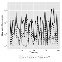
Figure 3: Filtering (left graph) and backward smoothing (right graph) for the toy example (6): gain factor as a function of $t$ for the estimation of $\mathbb{E}[x_{t}|y_{0:t}]$ and for the estimation of $\mathbb{E}[x_{t}|y_{0:T}]$, obtained from 500 independent runs of SQMC and SMC.

5.2 Example 2: Multivariate stochastic volatility model

We consider the following multivariate stochastic volatility model (SV) proposed by Chan et al., (2006):

$$\begin{cases}\mathbf{y}_{t}=S_{t}^{1/2}\boldsymbol{\epsilon}_{t},\quad&t\geq 0\\ \mathbf{x}_{t}=\boldsymbol{\mu}+\Phi(\mathbf{x}_{t-1}-\boldsymbol{\mu})+\Psi^{\frac{1}{2}}\boldsymbol{\nu}_{t},\quad&t>0\end{cases}$$ (7)

where $S_{t}=\text{diag}(\exp(x_{t1}),...,\exp(x_{td}))$, $\Phi$ and $\Psi$ are diagonal matrices and $(\boldsymbol{\epsilon}_{t},\boldsymbol{\nu}_{t})\sim\mathcal{N}_{2d}(\bm{0}_{2d},C)$, with $C$ a correlation matrix and $\bm{0}_{2d}=(0,\dots,0)\in\mathbb{R}^{2d}$.

In order to study the relative performance of SQMC over SMC as the dimension $d$ of the hidden process increases we perform simulations for $d\in\{1,2,4,10\}$. The parameters we use for the simulations are the same as in Chan et al., (2006): $\phi_{ii}=0.9$, $\mu_{i}=-9$, $\psi_{ii}^{2}=0.1$ for all $i=1,...,d$ and

$$C=\begin{pmatrix}0.6\mathbf{1}_{d}+0.4\mathcal{I}_{d}&-0.1\mathbf{1}_{d}-0.2\mathcal{I}_{d}\\ -0.1\mathbf{1}_{d}-0.2\mathcal{I}_{d}&0.8\mathbf{1}_{d}+0.2\mathcal{I}_{d}\end{pmatrix}$$

where $\mathcal{I}_{d}$ is the $d$-dimensional identity matrix, and $\mathbf{1}_{d}$ is the $d\times d$ matrix having one in all its entries. Note that the errors terms $\boldsymbol{\epsilon}_{t}$ and $\boldsymbol{\nu}_{t}$ are correlated so that the weight function $G_{t}$ depends now both on $\mathbf{x}_{t-1}$ and on $\mathbf{x}_{t}$. The prior distribution for $\mathbf{x}_{0}$ is the stationary distribution of the process $(\mathbf{x}_{t})$ and we take $T=399$.

$d=1$	$d=2$
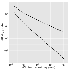
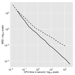
$d=4$

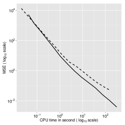
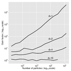
Figure 4: Log-likelihood estimation of SV model (7): MSE as a function of CPU time, for $d=1$, 2, 4; gain factor as a function of $N$ for $d=1$, 2, 4 and 10. The solid lines are for SQMC while the dashed lines are for SMC. The graphs are obtained from 200 independent runs of SQMC and SMC.

The three first panels of Figure 4 present results for the estimation of the log-likelihood (evaluated at the true value of the parameters and for the complete dataset $y_{0:T}$), for $d\in\{1,2,4\}$. One sees that the gain factor increases quickly with $N$, and, more importantly, the MSE of SQMC converges faster than SMC even as a function of CPU time. In fact, except for a very small interval for the univariate model, SQMC always outperforms SMC in terms of MSE for the same CPU effort. We note the particularly impressive values of the gain factor we obtain for $d=1$ when $N$ is large: around $4.2\times 10^{4}$ for $N=2^{17}$. The last panel of Figure 4 plots the gain factors as a function of $N$, for same values of $d$, plus $d=10$. The improvement brought by SQMC decreases with the dimension, and in fact, for $d=10$, the gain factor is essentially one for the considered values of $N$; yet for $d=4$ we still observe some notable improvement; e.g. a gain factor of 10 for $N\approx 10^{5}$. We now focus on $d=1$, 2 and 4.

Figure 5 represents the evolution with respect to $t$ of the MSE for the partial log-likelihood of data $y_{0:t}$ up to time $t$; gain factors are reported for different values of $N$. As we can see from these graphs, the performance of SQMC does not seem to depreciate with $t$.

Finally, Figure 6 shows that SQMC also give impressive gain when $d>1$ concerning the estimation of the filtering expectation $\mathbb{E}[x_{1t}|\mathbf{y}_{0:t}]$ of the first component of $\mathbf{x}_{t}$.

Univariate SV model
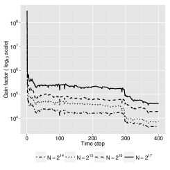
Bivariate SV model
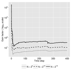
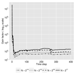
Four dimensional SV model

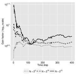
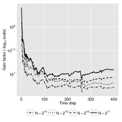
Figure 5: Log-likelihood estimation of the SV model (7): gain factor as a function of $t$, obtained from 200 independent runs of SQMC and SMC.

Bivariate SV model	Four dimensional SV model

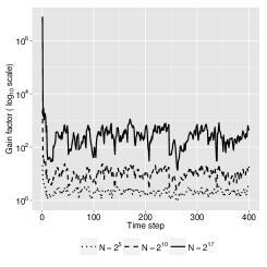
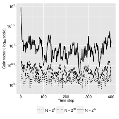
Figure 6: Filtering of the multivariate SV model (7): gain factor as a function of $t$ for the estimation of $\mathbb{E}[x_{1t}|\mathbf{y}_{0:t}]$, obtained from 200 independent runs of SQMC and SMC.

5.3 Application: Bayesian estimation of MSV using PMMH on real data

To compare SMC to SQMC when used as a way to approximate the likelihood within a PMMH algorithm, as described in Section 4.1, we turn our attention to the Bayesian estimation of the multivariate SV model (7), for $d=2$. As in Chan et al., (2006), we take the following prior:

$$\phi_{ii}\sim\mathcal{U}((0,1)),\quad 1/\psi^{2}_{ii}\sim\mathrm{Gamma}(10\exp(-10),10\exp(-3))\quad i=1,\dots d,$$

where $\phi_{ii}$ and $\psi^{2}_{ii}$ denotes respectively the diagonal elements of $\Phi$ and $\Psi$, and a flat prior for $\bm{\mu}$. In addition, we assume that $C$ is uniformly distributed on the space of correlation matrices which are such that the errors terms $\boldsymbol{\epsilon_{t}}$ and $\boldsymbol{\nu_{t}}$ are independents (no leverage effects). To sample from the posterior distribution of the parameters we use a Gaussian random walk Metropolis-Hastings algorithm with covariance matrix $\Sigma$ calibrated so that the acceptance probability of the algorithm becomes, as $N\rightarrow+\infty$, close to 25%. The matrix $\Sigma$, as well as the starting point of the Markov chain, are calibrated using a pilot run of the algorithm with $\Sigma=0.011^{2}\mathcal{I}_{8}$ and starting at the value of the parameters we used above for the simulations. To compare PMMH-SQMC with PMMH-SMC, we run the two algorithms during $10^{5}$ iterations and for values of $N$ ranging from 10 to 200, where $N$ increases from 10 to 100 by increment of 10 and then by increment of 50.

We consider the following dataset: the two series are the mean-corrected daily return on the Nasdaq and S&P 500 indices for the period ranging from the $3^{\text{rd}}$ January 2012 to the 21${}^{\text{th}}$ October 2013 so that the data set contains $452$ observations.

Figure 7 shows the Metropolis-Hastings acceptance rate and the effective sample sizes (see Robert and Casella,, 2004, Section 12.3.5, for a definition) for the PMMH-SQMC algorithm and for the standard PMMH algorithm. We first observe that the acceptance rate of PMMH-SQMC increases very quickly with $N$. Indeed, it is already of 20% for only 30 particles while for the same number of particles the acceptance rate for the standard PMMH is approximatively 6.5%. As far as the acceptance rate is concerned, there is no significant gain to take $N>60$ for the PMMH-SQMC algorithm while for the plain Monte Carlo algorithm the acceptance rate is only about 20% for $N=200$ and therefore much smaller than the target of 25%. Looking at the results for the effective sample sizes (ESSs), we see that the same conclusions hold. More precisely, for the PMMH-SQMC algorithm, the ESSs increase with $N$ much faster than for PMMH-SMC. Indeed, for $N\in 10:50$, the ESSs for the former is between 2.18 and 14.94 times larger than for PMMH-SMC.

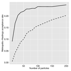
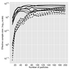
Figure 7: Metropolis-Hastings acceptance rate and effective sample sizes (one per parameter) for the multivariate SV model (7), $d=2$, and real data: the solid lines are for PMMH-SQMC while the dashed ones are for PMMH-SMC. The results are obtained from a Markov Chain of length $10^{5}$.

5.4 Example 3: Neural decoding

Neural decoding models are used for brain-machine interface in order to make inference about an organism’s environment from its neural activity. More precisely, we consider the problem of decoding a set of environment variables $\mathbf{p}_{t}\in\mathbb{R}^{2}$, from the firing ensemble of $d_{y}$ neurons. The latent vector $\mathbf{p}_{t}$ may be interpreted as two-dimensional hand kinetics for motor cortical decoding (see Koyama et al.,, 2010, and references therein for more details about neural decoding models). Noting $\dot{\mathbf{p}}_{t}$ the vector of velocities, the neural decoding model we consider is given by (Koyama et al.,, 2010)

$$\begin{cases}y_{ti}|\mathbf{x}_{0:t}\sim\mathcal{P}\left(\Delta\exp(\alpha_{i}+\beta^{T}_{i}\mathbf{x}_{t})\right),&i\in 1:d_{y},\quad\hskip 41.82558ptt\geq 0\\ \mathbf{x}_{t}=\Phi\mathbf{x}_{t-1}+\Psi\boldsymbol{\epsilon}_{t},&\boldsymbol{\epsilon}_{t}\sim\mathcal{N}_{2}(\bm{0}_{2},\sigma^{2}\mathcal{I}_{2}),\quad t>0\end{cases}$$ (8)

and $\mathbf{x}_{0}\sim\mathcal{N}_{4}(\bm{0}_{4},\mathcal{I}_{4})$, where $\mathbf{x}_{t}=(\mathbf{p}_{t},\dot{\mathbf{p}}_{t})$, the $y_{ti}$’s are conditionally independent, $\mathcal{P}(\lambda)$ denotes the Poisson distribution with parameter $\lambda$, $\Delta$ is the duration of the interval over which spikes are counted at each time step, and

$$\Phi=\begin{pmatrix}\mathcal{I}_{2}&\Delta\mathcal{I}_{2}\\ \boldsymbol{0}_{2}&\mathcal{I}_{2}\end{pmatrix},\quad\Psi^{T}=\begin{pmatrix}0&0&1&0\\ 0&0&0&1\end{pmatrix}.$$

Realistic values for the parameters, see Koyama et al., (2010), that we will take in ours simulations, are $d_{y}=10$, $T=23$, $\Delta=0.03$, $\sigma^{2}=0.019$, $\alpha_{i}{\buildrel i.i.d\over{\sim}}\mathcal{N}_{1}(2.5,1)$, $\beta_{i}\sim\mathcal{U}([0,1)^{d})$.

One important aspect of this model is that the dimension of the noise term $\boldsymbol{\epsilon}_{t}$ is lower than the dimension of $\mathbf{x}_{t}$. As a result, two components of $\mathbf{x}_{t}$ are deterministic functions of $\mathbf{x}_{t-1}$. Many tracking problems have a similar structure.

This requires us to slightly adapt SQMC as follows: one samples jointly the ancestor variables $a_{t-1}^{1:N}$ and the new velocities $\dot{\mathbf{p}}_{t}^{n}$ as in Steps (b) and (c) of Algorithm 3, then one obtains the new $\mathbf{p}_{t}^{n}$ as $\mathbf{p}_{t}^{n}=\mathbf{p}_{t-1}^{n}+\dot{\mathbf{p}}_{t}^{n}$, i.e. the deterministic linear transformation of $\mathbf{p}_{t-1}^{a_{t-1}^{n}}$ and $\dot{\mathbf{p}}_{t-1}^{n}$ defined by the model. Note that in this case the dimension of the point set $\mathbf{u}_{t}^{1:N}$ is 3 for $t>0$; we could say that $d=2$ in this case, even if the dimension of $\mathbf{x}_{t}$ itself is $4$.

Figures 8 and 9 present, respectively, results for the estimation of the log-likelihood (evaluated at the true value of the parameters) and for the estimation of the filtering expectation $\mathbb{E}[x_{ti}|\mathbf{y}_{0:t}]$ for $i\in 1:d$. Concerning the log-likelihood estimation we observe fast increase of the gain factor after about $2^{11}$ particles with a maximum close to 21 when $N$ is very large. The gain of SQMC compensates its longer running time after only about $0.17$ seconds. Important and increasing (in $N$) gains are also observed for the estimation of the filtering expectations.

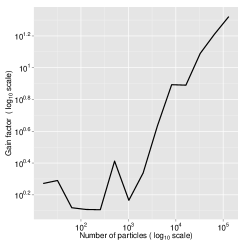
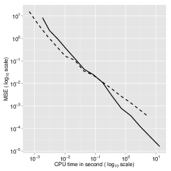
Figure 8: Log-likelihood estimation of the neural decoding model (8). The left graph gives the ratio of the SMC and the SQMC MSE. In the right graph, the solid line is for SQMC while the dashed line is for SMC. The graphs are obtained from 200 independent runs of SQMC and SMC.

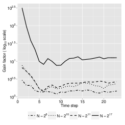
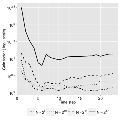
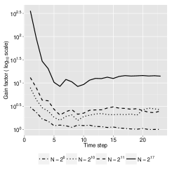
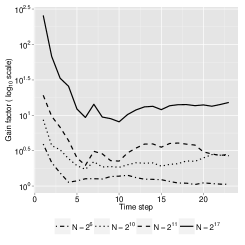
Figure 9: Filtering of the Neuro decoding model (8). From left to right and from top to bottom, the graphs give the ratio of the SMC and SQMC MSE for the estimation of $\mathbb{E}[x_{kt}|\mathbf{y}_{0:t}]$ as a function of $t$, $k=1,\dots,4$, and are obtained from 200 independent runs of SQMC and SMC.

6 Conclusion and future work

The main message of the paper is that SMC users should be strongly encouraged to switch to SQMC, as SQMC is “typically” much more accurate (produces estimates with smaller errors) than SMC. We add the word “typically” to recall that our asymptotic analysis, by construction, proves only that the SQMC error is smaller than the SMC error for $N$ large enough. But our range of numerical examples, which are representative of real-world filtering problems, makes us optimistic than in most practical cases SQMC should outperform SMC even for moderate values of $N$.

The main price to pay to switch to SQMC is that users should spend some time thinking on how to write the simulation of $\mathbf{x}_{t}^{n}$ given $\mathbf{x}_{t-1}^{n}$ as $\mathbf{x}_{t}^{n}=\Gamma_{t}(\mathbf{x}_{t-1}^{n},\mathbf{u}_{t}^{n})$, where $\mathbf{u}_{t}^{n}\sim\mathcal{U}([0,1]^{d})$ and $\Gamma_{t}$ is a deterministic function that is easy to evaluate. Fortunately, this is often straightforward. In fact, there are many models of interest where $\mathbf{x}_{t}^{n}$ given $\mathbf{x}_{t-1}^{n}$ is linear and Gaussian. Since this case is already implemented in our program, adapting it to such a model should be just a matter of changing a few lines of code (to evaluate the probability density of $\mathbf{y}_{t}$ given $\mathbf{x}_{t}$).

Regarding future work, the most pressing tasks seem (a) to refine the convergence rate of the SQMC error; and (b) to establish that it does not degenerate over time (in the spirit of time-uniform estimates for SMC, see p. 244 of Del Moral,, 2004). Regarding the former, He2014 make the interesting conjecture that the mean square error of SQMC converges at rate $\mathcal{O}(N^{-1-2/d})$. This would explain why the relative performance of SQMC decreases with the dimension. Fortunately, a majority of the state space models of interest in signal processing, finance, or other fields are such that $d\leq 6$. A notable exception is geophysical data assimilation (in e.g. meteorology or oceanography) for which $d$ can be very large, but for such large-dimensional problems SMC seems to perform too poorly for practical use anyway (Bocquet et al.,, 2010).

Finally, it is also our hope that this paper will help QMC garner wider recognition in Bayesian computation and related fields. Granted, QMC is more technical than standard Monte Carlo, and there is perhaps something specific about particle filtering that makes the introduction of QMC so effective. Yet we cannot help but think that the full potential of QMC in Statistics remains under-explored.

Appendix A Proofs

A.1 Importance sampling: Theorems 1 and 2

A.1.1 Preliminary calculation

Let $\hat{q}(\mathrm{d}\mathbf{x})=\mathcal{S}(\mathbf{x}^{1:N})(\mathrm{d}\mathbf{x})=N^{-1}\sum_{n=1}^{N}\delta_{\mathbf{x}^{n}}(\mathrm{d}\mathbf{x})$, and, as a preliminary calculation, take $\varphi\in L_{2}\left([0,1)^{d},\lambda_{d}\right)$ and

$$\left|\pi^{N}(\varphi)-\pi(\varphi)\right| =\left|\frac{N^{-1}\sum_{n=1}^{N}w(\mathbf{x}^{n})\varphi(\mathbf{x}^{n})}{N^{-1}\sum_{n=1}^{N}w(\mathbf{x}^{n})}-\pi(\varphi)\right|$$

$$\leq\left|\frac{N^{-1}\sum_{n=1}^{N}w(\mathbf{x}^{n})\varphi(\mathbf{x}^{n})}{N^{-1}\sum_{n=1}^{N}w(\mathbf{x}^{n})}-N^{-1}\sum_{n=1}^{N}w(\mathbf{x}^{n})\varphi(\mathbf{x}^{n})\right|$$

$$\quad+\left|N^{-1}\sum_{n=1}^{N}w(\mathbf{x}^{n})\varphi(\mathbf{x}^{n})-q(w\varphi)\right|$$

$$\leq\frac{N^{-1}\sum_{n=1}^{N}w(\mathbf{x}^{n})\left|\varphi(\mathbf{x}^{n})\right|}{N^{-1}\sum_{n=1}^{N}w(\mathbf{x}^{n})}\left|q(w)-\hat{q}(w)\right|$$

$$\quad+\left|\hat{q}(w\varphi)-q(w\varphi)\right|.$$ (9)

We will use this inequality in the two following proofs.

A.1.2 Proof of Theorem 1

Take $\varphi=\mathds{1}_{B}$ for $B\in\mathcal{B}_{[0,1)^{d}}$ in (9). Consider the first term above. The ratio is bounded by $1$, and (since $w$ is bounded) $\left|q(w)-\hat{q}(w)\right|\rightarrow 0$ by portmanteau lemma (Van der Vaart,, 2007, Lemma 2.2). Now consider the second term.

We follow essentially the same steps as in Van der Vaart, (2007, Lemma 2.2). Without loss of generality we assume that $q(\mathrm{d}\mathbf{x})$ is a continuous probability measure (the same argument as in Van der Vaart,, 2007, is used for the general case).

Let $\epsilon>0$ and take $J\in\mathcal{B}_{[0,1)^{d}}$ such that $q(J^{c})\leq\epsilon$. Since $J$ is compact, $w(\cdot{})$ is uniformly continuous on $J$. Let $\eta>0$ be such that $\|\mathbf{x}-\mathbf{y}\|\leq\eta\implies|w(\mathbf{x})-w(\mathbf{y})|\leq\epsilon$, $\forall(\mathbf{x},\mathbf{y})\in J^{2}$. Let $\{J_{k}\}_{k=1}^{m}$ be a split of $J$ into a finite collection of $m$ closed hyperrectangles with radius (at most) $\eta$. Let $g(\mathbf{x})=\sum_{k=1}^{m}w(\mathbf{x}_{k})\mathbb{I}_{J_{k}}(\mathbf{x})$ and note that $|w(\mathbf{x})-g(\mathbf{x})|\leq 2^{d}\epsilon$, $\forall\mathbf{x}\in J$. Thus

$$\left|\int_{B}w(\mathbf{x})\left\{\hat{q}(\mathrm{d}\mathbf{x})-q(\mathrm{d}\mathbf{x})\right\}\right| \leq\left|\int_{B}\left\{w(\mathbf{x})-g(\mathbf{x})\right\}\hat{q}(\mathrm{d}\mathbf{x})\right|+\left|\int_{B}g(\mathbf{x})\left\{\hat{q}(\mathrm{d}\mathbf{x})-q(\mathrm{d}\mathbf{x})\right\}\right|$$

$$\quad+\left|\int_{B}\left\{w(\mathbf{x})-g(\mathbf{x})\right\}q(\mathrm{d}\mathbf{x})\right|$$

where for the first term we have

$$\left|\int_{B}(w(\mathbf{x})-g(\mathbf{x}))\hat{q}(\mathrm{d}\mathbf{x})\right| \leq\left|\int_{B\cap J}(w(\mathbf{x})-g(\mathbf{x}))\hat{q}(\mathrm{d}\mathbf{x})\right|+\left|\int_{B\cap J^{c}}w(\mathbf{x})\hat{q}(\mathrm{d}\mathbf{x})\right|$$

$$\leq 2^{d}\epsilon+\|w\|_{\infty}\hat{q}(J^{c})$$

$$\leq\epsilon(2^{d}+2\|w\|_{\infty})$$ (10)

as $\hat{q}(J^{c})$ converges to $q(J^{c})$, and thus $\hat{q}(J^{c})\leq 2\epsilon$ for $N$ large enough; and for the second term

$$\begin{split}\left|\int_{B}g(\mathbf{x})\left\{\hat{q}(\mathrm{d}\mathbf{x})-q(\mathrm{d}\mathbf{x})\right\}\right|&\leq\sum_{k=1}^{m}w(\mathbf{x}_{k})\left|\int_{\bar{J}_{k}\cap B}\left\{\hat{q}(\mathrm{d}\mathbf{x})-q(\mathrm{d}\mathbf{x})\right\}\right|\\ &\leq\|\hat{q}(\mathrm{d}\mathbf{x})-q(\mathrm{d}\mathbf{x})\|_{\mathrm{E}}\sum_{k=1}^{m}w(\mathbf{x}_{k}).\end{split}$$ (11)

Finally, for the third term:

$$\left|\int_{B}\left\{w(\mathbf{x})-g(\mathbf{x})\right\}q(\mathrm{d}\mathbf{x})\right| \leq\left|\int_{B\cap J}\left\{w(\mathbf{x})-g(\mathbf{x})\right\}q(\mathrm{d}\mathbf{x})\right|+\left|\int_{B\cap J^{c}}w(\mathbf{x})q(\mathrm{d}\mathbf{x})\right|$$

$$\leq\epsilon(2^{d}+\|w\|_{\infty}).$$ (12)

Putting (10)-(12) together shows that, for all $B\in\mathcal{B}_{[0,1)^{d}}$

$$\left|\int_{B}w(\mathbf{x})\left\{\hat{q}(\mathrm{d}\mathbf{x})-q(\mathrm{d}\mathbf{x})\right\}\right| \leq\epsilon(2^{d+1}+3\|w\|_{\infty})+\|\hat{q}(\mathrm{d}\mathbf{x})-q(\mathrm{d}\mathbf{x})\|_{\mathrm{E}}\sum_{k=1}^{m}w(\mathbf{x}_{k})$$

$$\leq\epsilon(2^{d+2}+3\|w\|_{\infty})$$ (13)

for $N$ large enough (as $\|\hat{q}(\mathrm{d}\mathbf{x})-q(\mathrm{d}\mathbf{x})\|_{\mathrm{E}}\rightarrow 0$) which concludes the proof of Theorem 1.

A.1.3 Proof of Theorem 2

We prove first $L_{1}$ convergence (first part of Theorem 2). We start again from (9), but for any $\varphi\in L_{2}\left([0,1)^{d},\lambda_{d}\right)$. For the second term, by Jensen’s inequality

$$\mathbb{E}\left|\hat{q}(w\varphi)-q(w\varphi)\right|\leq\left[\mathrm{Var}\left\{\hat{q}(w\varphi)\right\}\right]^{1/2}=\mathcal{O}(r(N)^{1/2})$$

by assumption. For the first term, using Cauchy-Schwartz, $\mathbb{E}(\left|CD\right|)\leq\left\{\mathbb{E}(C^{2})\mathbb{E}(D^{2})\right\}^{1/2}$ with

$$C=\frac{N^{-1}\sum_{n=1}^{N}w(\mathbf{x}^{n})\left|\varphi(\mathbf{x}^{n})\right|}{N^{-1}\sum_{n=1}^{N}w(\mathbf{x}^{n})},\quad D=q(w)-\hat{q}(w),$$

we have $\left\{\mathbb{E}(D^{2})\right\}^{1/2}=\mathcal{O}(r(N)^{1/2})$, and what remains to prove is that $\mathbb{E}(C^{2})=\mathcal{O}(1)$.

From (13), and under Assumption 2, one sees that there exists $N_{\epsilon}$ such that with probability one $N^{-1}\sum_{n=1}^{N}w(\mathbf{x}^{n})\geq 1/2$ as soon as $N\geq N_{\epsilon}$. Under Assumption 1, a bound similar to (13) is easily obtained by replacing $\mathbf{x}^{1:N}$ with $\mathbf{u}^{1:N}$ and observing that $w\circ F_{q}^{-1}$ is continuous and bounded. Thus, for $N$ large enough

$$\mathbb{E}(C^{2})\leq 4\mathbb{E}\left\{\left[N^{-1}\sum_{n=1}^{N}w(\mathbf{x}^{n})\left|\varphi(\mathbf{x}^{n})\right|\right]^{2}\right\}\leq\mathcal{O}(r(N))+\pi(\left|\varphi\right|)^{2}=\mathcal{O}(1).$$

We now prove $L_{2}$ convergence (second part of Theorem 2):

$$\mathrm{Var}\left\{\pi^{N}(\varphi)\right\}\leq\left[\text{Var}\left\{\pi^{N}(\varphi)-\hat{q}(w\varphi)\right\}^{1/2}+\text{Var}\left\{\hat{q}(w\varphi)\right\}^{1/2}\right]^{2},$$

with $\text{Var}\left\{\hat{q}(w\varphi)\right\}=\mathcal{O}(r(N))$ by assumption, and for the first term:

$$\mathbb{E}\left[\left\{\pi^{N}(\varphi)-\hat{q}(w\varphi)\right\}^{2}\right]= \mathbb{E}\left[\left\{\sum_{n=1}^{N}\left\{W^{n}-N^{-1}w(\mathbf{x}^{n})\right\}\varphi(\mathbf{x}^{n})\right\}^{2}\right]$$

$$= \mathbb{E}\left[\left\{1-N^{-1}\sum_{n=1}^{N}w(\mathbf{x}^{n})\right\}^{2}\left\{\sum_{n=1}^{N}W^{n}\varphi(\mathbf{x}^{n})\right\}^{2}\right]$$

$$= \mathbb{E}\left[\frac{\left\{1-\hat{q}(w)\right\}^{2}\hat{q}(w\varphi)^{2}}{\hat{q}(w)^{2}}\right]$$

$$\leq 4\mathbb{E}\left[\left\{1-\hat{q}(w)\right\}^{2}\hat{q}(w\varphi)^{2}\right]$$

for $N$ large enough, using the same argument as above (as $\hat{q}(w)\rightarrow 1$). Then

$$\mathbb{E}\left[\left\{1-\hat{q}(w)\right\}^{2}\hat{q}(w\varphi)^{2}\right]\leq \mathbb{E}\left[\left\{1-\hat{q}(w)\right\}^{2}\left\{\hat{q}(w\varphi)-\pi(\varphi)\right\}^{2}\right]-\pi(\varphi)^{2}\mathbb{E}\left[\left\{1-\hat{q}(w)\right\}^{2}\right]$$

$$+2|\pi(\varphi)|\mathbb{E}\left[|\hat{q}(w\varphi)|\left\{1-\hat{q}(w)\right\}^{2}\right]$$

where for the second term, $\mathbb{E}\left[\left\{1-\hat{q}(w)\right\}^{2}\right]=\mathrm{Var}\left[\hat{q}(w)\right]=\mathcal{O}\left(r(N)\right)$, for the first term

$$\mathbb{E}\left[\left\{1-\hat{q}(w)\right\}^{2}\left\{\hat{q}(w\varphi)-\pi(\varphi)\right\}^{2}\right] =\mathbb{E}\left[\left\{1-\hat{q}(w)\right\}^{2}\left\{\hat{q}(w\varphi)-q(w\varphi)\right\}^{2}\right]$$

$$\leq(1+\|w\|_{\infty})^{2}\mathrm{Var}\left[\hat{q}(w\varphi)\right]$$

$$=\mathcal{O}\left(r(N)\right)$$

and finally for the third term

$$\mathbb{E}\left[|\hat{q}(w\varphi)|\left\{1-\hat{q}(w)\right\}^{2}\right]\leq \mathbb{E}\left[|\hat{q}(w\varphi)-q(w\varphi)|\left\{1-\hat{q}(w)\right\}^{2}\right]+|q(w\varphi)|\mathrm{Var}\left[\hat{q}(w)\right]$$

with

$$\mathbb{E}\left[|\hat{q}(w\varphi)-q(w\varphi)|\left\{1-\hat{q}(w)\right\}^{2}\right] \leq\left(1+\|w\|_{\infty}\right)\mathrm{Var}\left[\hat{q}(w\varphi)\right]^{1/2}\mathrm{Var}\left[\hat{q}(w)\right]^{1/2}$$

$$=\mathcal{O}\left(r(N)\right)$$

which concludes the proof.

For subsequent uses (see the proof of Theorem 6), we note that these computations imply, for $N$ large enough,

$$\mathrm{Var}\{\pi^{N}(\varphi)\}\leq\left\{2(1+\|w\|_{\infty})\mathrm{Var}[\hat{q}(w\varphi)]^{1/2}+(1-2|\pi(\varphi)|)\mathrm{Var}[\hat{q}(w)]^{1/2}\right\}^{2}$$ (14)

$$|\pi^{N}(\varphi)-\pi(\varphi)|\leq[\mathrm{Var}\{\hat{q}(w\varphi)\}]^{1/2}+2[\mathrm{Var}\{\hat{q}(w)\}]^{1/2}\left[\mathrm{Var}\{\hat{q}(w\varphi)\}+\pi(|\varphi|)^{2}\right]^{1/2}.$$ (15)

A.2 Hilbert curve and discrepancy: Theorems 3 and 4

The proofs in this section rely on the properties of the Hilbert curved laid out in Section 2.3 and the corresponding notations.

A.2.1 Theorem 3

We first show that $\|\pi_{h}^{N}-\pi_{h}\|_{\mathrm{E}}=\sup_{0\leq a<b\leq 1}|\pi_{h}^{N}([a,b))-\pi_{h}([a,b))|$. Because $\pi_{h}$ is a continuous probability measure on $[0,1)$, the result is obvious if $\pi_{h}^{N}$ is continuous as well. Let $0\leq a<b<1$ be such that $b$ is a discontinuity point of $F_{\pi_{h}^{N}}$ and let $\delta>0$ be small enough so that $\pi_{h}^{N}([a,b])=\pi_{h}^{N}([a,b+\delta))$ and $b+\delta\leq 1$. Then,

$$\Big{|}|\pi_{h}^{N}([a,b])-\pi_{h}([a,b])|-|\pi_{h}^{N}([a,b+\delta))-\pi_{h}([a,b+\delta))|\Big{|}\leq\pi_{h}([b,b+\delta]).$$

By the bi-measure property of the Hilbert curve, the set $H([b,b+\delta])$ has Lebesgue measure $\delta$ in $[0,1)^{d}$ and therefore, $\pi_{h}([b,b+\delta])=\pi\big{(}H[b,b+\delta])\big{)}\leq\|\pi\|_{\infty}\delta$ where $\|\pi\|_{\infty}<+\infty$ by assumption. Hence, for all $\epsilon>0$ small enough,

$$\left|\|\pi_{h}^{N}-\pi_{h}\|_{\mathrm{E}}-\sup_{0\leq a<b\leq 1}|\pi_{h}^{N}([a,b))-\pi_{h}([a,b))|\right|\leq\epsilon.$$

To prove the theorem note that the above computations imply that

$$\|\pi_{h}^{N}-\pi_{h}\|_{\mathrm{E}} \leq 2\sup_{b\in(0,1)}|\pi_{h}^{N}([0,b])-\pi_{h}([0,b])|.$$

To bound the right-hand side, let $I=[0,b]$, $b\in(0,1)$, and $m\in\mathbb{N}$ (which may depend on $N$) and assume first that $b\geq 2^{-dm}$, so that $I_{m}^{d}(0)\subseteq I$. Take $\tilde{I}=[0,k^{*}2^{-dm}]$, where $k^{*}\leq(2^{dm}-1)$ is the largest integer such that $k^{*}2^{-dm}\leq b$. Then

$$\left|\pi_{h}^{N}(I)-\pi_{h}(I)\right| \leq\left|F_{\pi_{h}^{N}}\left(k^{*}2^{-dm}\right)-F_{\pi_{h}}\left(k^{*}2^{-dm}\right)\right|$$

$$+\left|\pi_{h}^{N}(I)-F_{\pi_{h}^{N}}\left(k^{*}2^{-dm}\right)-\left\{\pi_{h}(I)-F_{\pi_{h}}\left(k^{*}2^{-dm}\right)\right\}\right|$$

$$=\left|\pi^{N}(J)-\pi(J)\right|+\left|\pi_{h}^{N}\left((k^{*}2^{-dm},b]\right)-\pi_{h}\left((k^{*}2^{-dm},b]\right)\right|$$ (16)

with $J=H(\tilde{I})$. Since $\tilde{I}$ is the union of $k^{*}$ intervals in $\mathcal{I}_{m}^{d}$, $J$ is the union of $k^{*}$ hypercubes in $\mathcal{S}_{m}^{d}$, and therefore (using a similar argument as above and Niederreiter,, 1992, Proposition 2.4),

$$\left|\pi^{N}(J)-\pi(J)\right| \leq c\|\pi^{N}-\pi\|_{\mathrm{E}}\leq 2^{dm}r(N)$$

for a constant $c$ and where $r(N)=\|\pi^{N}-\pi\|_{\mathrm{E}}.$

For the second term of (16), by the properties of the Hilbert curve,

$$\left|\pi_{h}^{N}\left((k2^{-dm},b]\right)-\pi_{h}\left((k2^{-dm},b]\right)\right| \leq\pi_{h}^{N}\left(I_{m}^{d}(k)\right)+\pi_{h}\left(I_{m}^{d}(k)\right)$$

$$=\pi^{N}\left(S_{m}^{d}(k)\right)+\pi\left(S_{m}^{d}(k)\right)$$

$$\leq 2\pi\left(S_{m}^{d}(k)\right)+r(N)$$

$$=\mathcal{O}\left(2^{-dm}\vee r(N)\right)$$

where the last inequality comes from the fact that $\pi(\mathbf{x})$ is a bounded density.

In case $b<2^{-dm}$, similar computations show that

$$\left|\pi_{h}^{N}(I)-\pi_{h}(I)\right|\leq\pi_{h}^{N}(I_{m}^{d}(0))+\pi_{h}(I_{m}^{d}(0))=\mathcal{O}\left(2^{-dm}\vee r(N)\right).$$

To conclude, we choose $m$ so that $2^{-dm}=\mathcal{O}(r(N)^{1/2})$, which gives

$$\sup_{b\in(0,1)}\left|\pi_{h}^{N}([0,b])-\pi_{h}([0,b])\right|=\mathcal{O}\left(r(N)^{1/2}\right).$$

Finally, since replacing $[0,b]$ by $[0,a)$ changes nothing to the proof of the result above, one may conclude that $\sup_{I\in\mathcal{B}_{[0,1)}}|\pi_{h}^{N}(I)-\pi_{h}(I)|=\mathcal{O}(r(N)^{1/2})$.

A.2.2 Proof of Theorem 4

Preliminary computations

The proof of this result is based on Hlawka and Mück, (1972, “Satz 2”). Compared to this latter, the main technical difficulty comes from the fact that the Rosenblatt transformation $F_{\pi_{h}^{N}\otimes K_{h}}$ is not continuous because $\pi_{h}^{N}$ is a weighted sum of Dirac measures. To control the “jumps” of the inverse Rosenblatt transformation $F^{-1}_{\pi_{h}^{N}\otimes K_{h}}$ introduced by the discontinuity of $\pi_{h}^{N}$, we first prove the following Lemma.

Lemma 9.

Consider the set-up of Theorem 4. For $n\in 1{:}N$, let $h_{1}^{n}=H(\mathbf{x}^{n}_{1})$ and assume that the points $h_{1}^{1:N}$ are labelled so that $n<m\implies h_{1}^{n}<h_{1}^{m}$. (Note that the inequality is strict because, by Assumption 2 of Theorem 4, the points $\mathbf{x}^{1:N}$ are distinct.) Without loss of generality, assume that $h_{1}^{1}>0$ and let $h_{1}^{0}=0$. Then, as $N\rightarrow+\infty$,

$$\max_{n\in 1:N}|h_{1}^{n}-h_{1}^{n-1}|\rightarrow 0.$$

To prove this Lemma, let $J_{N}=[h_{1}^{n^{*}-1},h_{1}^{n^{*}}]$ where $|h_{1}^{n^{*}}-h_{1}^{n^{*}-1}|=\max_{n\in 1:N}|h_{1}^{n}-h_{1}^{n-1}|$. Since $J_{N}$ contains at most two points, we have

$$\pi_{h}(J_{N})\leq\pi_{h}^{N}(J_{N})+r_{2}(N)\leq 2r_{1}(N)+r_{2}(N)$$

where $r_{1}(N)=\max_{n\in 1:N}W_{N}^{n}$ and $r_{2}(N)=\|\pi_{h}^{N}-\pi_{h}\|_{\mathrm{E}}$; note $r_{1}(N)\rightarrow 0$ by Assumption 2 of Theorem 4 while $r_{2}(N)\rightarrow 0$ by Assumption 3 of Theorem 4 and by Theorem 3. Therefore, $\pi_{h}(J_{N})\rightarrow 0$ as $N\rightarrow+\infty$.

Assume now that $\max_{n\in 1:N}|h_{1}^{n}-h_{1}^{n-1}|\not\rightarrow 0$. Then, this means that there exists a $\epsilon\in(0,1)$ such that, for all $N>1$ there exists a $N^{*}\geq N$ for which $\lambda_{1}(J_{N^{*}})\geq\epsilon$. Assume first that $J_{N^{*}}\subset[0,1-\frac{\epsilon}{2}]$. In that case, we have $\pi_{h}(J_{N^{*}})\geq c_{\epsilon}$ for a constant $c_{\epsilon}>0$. Indeed, by the continuity of the Hilbert curve, the set $H([0,1-\frac{\epsilon}{2}])$ is compact and therefore, $\forall\mathbf{x}\in H([0,1-\frac{\epsilon}{2}])$, $\pi(\mathbf{x})\geq\underline{\pi}^{(\epsilon)}$ for a constant $\underline{\pi}^{(\epsilon)}>0$ because the density $\pi(\mathbf{x})$ is continuous and strictly positive. Therefore, if $J_{N^{*}}\subset[0,1-\frac{\epsilon}{2}]$, we have

$$\pi_{h}(J_{N^{*}})=\pi(H(J_{N^{*}}))\geq\underline{\pi}^{(\epsilon)}\lambda_{d}(H(J_{N^{*}}))=\underline{\pi}^{(\epsilon)}\lambda_{1}(J_{N^{*}})\geq\epsilon\underline{\pi}^{(\epsilon)}$$

where the second equality uses the bi-measure property of the Hilbert curve.

Assume now that $J_{N^{*}}\not\subset[0,1-\frac{\epsilon}{2}]$. Write $J_{N^{*}}=[a_{N^{*}},b_{N^{*}}]$ and note that, since $\lambda_{1}(J_{N^{*}})\geq\epsilon$, we have $a_{n}^{*}<1-\epsilon$ and therefore

$$\pi_{h}(J_{N^{*}})=\pi_{h}\left(\left[a_{N^{*}},1-\frac{\epsilon}{2}\right]\right)+\pi_{h}\left(\left(1-\frac{\epsilon}{2},b_{N^{*}}\right]\right)\geq\left(1-\frac{\epsilon}{2}-a_{N^{*}}\right)\underline{\pi}^{(\epsilon)}\geq\frac{\epsilon}{2}\underline{\pi}^{(\epsilon)}.$$

Thus, this shows that if $\max_{n\in 1:N}|h_{1}^{n}-h_{1}^{n-1}|\not\rightarrow 0$, then there exists a $\epsilon\in[0,1)$ such that $\limsup_{N\rightarrow+\infty}\pi_{h}(J_{N})\geq(\epsilon\underline{\pi}^{(\epsilon)})/2>0$. This contradicts the fact that $\pi_{h}(J_{N})\rightarrow 0$ as $N\rightarrow+\infty$ and the proof is complete.

Proof of Theorem 4

We use the shorthand $\alpha_{N}(B)=\mathcal{S}(\mathbf{u}^{1:N})(B)$ for any set $B\subset[0,1)^{1+d_{2}}$. One has

$$\|\mathcal{S}(P_{h}^{N})-\pi_{h}^{N}\otimes K_{h}\|_{\mathrm{E}}=\sup_{B\in\mathcal{B}^{N}_{[0,1)^{1+d_{2}}}}\left|\alpha_{N}\left(E^{N}(B)\right)-\lambda_{1+d_{2}}\left(E^{N}(B)\right)\right|$$

where

$$\mathcal{B}^{N}_{[0,1)^{1+d_{2}}}=\left\{B=[\bm{a},\bm{b}]\in\mathcal{B}_{[0,1)^{1+d_{2}}}:\min_{n\in 1:N}h(\mathbf{x}^{n}_{1})\leq F_{\pi_{h}^{N}}(b_{1})\leq\max_{n\in 1:N}h(\mathbf{x}^{n}_{1})\right\},$$

and where, for an arbitrary set $\tilde{B}=[a_{1},b_{1}]\times[\bm{a}^{\prime},\bm{b}^{\prime}]$ with $0\leq a_{1}\leq b_{1}<1$ and with $0\leq a_{i}^{\prime}\leq b_{i}^{\prime}<1$ for all $i\in 1:d_{2}$, we use the shorthand $E^{N}(\tilde{B})$ for the set

$$\left\{(u_{1},\mathbf{u}_{2})\in[0,1)^{1+d_{2}}:F_{\pi_{h}^{N}}(a_{1})\leq u_{1}\leq F_{\pi_{h}^{N}}(b_{1}),\mathbf{u}_{2}\in F_{K_{h}}\left(F^{-1}_{\pi_{h}^{N}}(u_{1}),[\bm{a}^{\prime},\bm{b}^{\prime}]\right)\right\}.$$

Let $\mathcal{P}$ be a partition of $[0,1)^{1+d_{2}}$ in $L^{d_{1}+d_{2}}$ congruent hyperrectanges $W$ of size $L^{-d_{1}}\times L^{-1}\times...\times L^{-1}$ where $L\geq 1$ is an arbitrary integer. Let $B=[a_{1},b_{1}]\times[\bm{a}^{\prime},\bm{b}^{\prime}]\in\mathcal{B}^{N}_{[0,1)^{1+d_{2}}}$, $\mathcal{U}_{1}$ the set of the elements of $\mathcal{P}$ that are strictly in $E^{N}(B)$, $\mathcal{U}_{2}$ the set of elements $W\in\mathcal{P}$ such that $W\cap\partial(E^{N}(B))\neq\varnothing$, $U_{1}=\cup\text{ }\mathcal{U}_{1}$, $U_{2}=\cup\text{ }\mathcal{U}_{2}$, and $U_{1}^{\prime}=E^{N}(B)\setminus U_{1}$ so that

$$\alpha_{N}\left(E^{N}(B)\right)-\lambda_{1+d_{2}}\left(E^{N}(B)\right)=\alpha_{N}(U_{1})-\lambda_{1+d_{2}}(U_{1})+\alpha_{N}(U_{1}^{\prime})-\lambda_{1+d_{2}}(U_{1}^{\prime}).$$

To bound $\alpha_{N}(U_{1}^{\prime})-\lambda_{1+d_{2}}(U_{1}^{\prime})$, note that we can cover $U_{1}^{\prime}$ with sets in $\mathcal{U}_{2}$, hence

$$\alpha_{N}(U_{1}^{\prime})-\lambda_{1+d_{2}}(U_{1}^{\prime})\leq\alpha_{N}(U_{2}),\quad\mbox{and }\alpha_{N}(U_{1}^{\prime})-\lambda_{1+d_{2}}(U_{1}^{\prime})\geq-\lambda_{1+d_{2}}(U_{2})$$

so that, by the definition of $D(\mathbf{u}^{1:N})$,

$$\left|\alpha_{N}(U_{1}^{\prime})-\lambda_{1+d_{2}}(U_{1}^{\prime})\right| \leq\left|\alpha_{N}(U_{2})-\lambda_{1+d_{2}}(U_{2})\right|+\lambda_{1+d_{2}}(U_{2})$$

$$\leq\#\mathcal{U}_{2}\left\{D(\mathbf{u}^{1:N})+L^{-(d_{1}+d_{2})}\right\}.$$

We therefore have

$$\left|\alpha_{N}\left(E^{N}(B)\right)-\lambda_{1+d_{2}}\left(E^{N}(B)\right)\right| \leq|\alpha_{N}(U_{1})-\lambda_{1+d_{2}}(U_{1})|+\#\mathcal{U}_{2}\left\{D(\mathbf{u}^{1:N})+L^{-(d_{1}+d_{2})}\right\}$$

$$\leq L^{d_{1}+d_{2}}D(\mathbf{u}^{1:N})+\#\mathcal{U}_{2}\left\{D(\mathbf{u}^{1:N})+L^{-(d_{1}+d_{2})}\right\}.$$

The rest of the proof is dedicated to bounding $\#\mathcal{U}_{2}$, the number of hyperrectangles in $\mathcal{P}$ required to cover $\partial\left(E^{N}(B)\right)$. To that effect, first note that, using the continuity of $F_{K_{h}}$ and the fact that $B$ and $E^{N}(B)$ are closed sets, we can easily show that $E^{N}(\partial(B))\subset\partial(E^{N}(B))$. Let $\#\mathcal{U}^{(1)}_{2}$ and $\#\mathcal{U}_{2}^{(2)}$ be, respectively, the number of hyperrectangles in $\mathcal{P}$ we need to cover $E^{N}(\partial(B))$ and to cover $P(B):=\partial(E^{N}(B))\setminus E^{N}(\partial(B))$. Hence, $\#\mathcal{U}_{2}\leq\#\mathcal{U}^{(1)}_{2}+\#\mathcal{U}^{(2)}_{2}$ and we now bound $\#\mathcal{U}^{(i)}_{2}$, $i\in 1:2$.

To bound $\#\mathcal{U}^{(1)}_{2}$ we first cover $\partial(B)$ with hyperrectangles belonging to a partition $\mathcal{P}^{\prime}$ of the set $[0,1)^{1+d_{2}}$. We construct $\mathcal{P}^{\prime}$ as a partition of the set $[0,1)^{1+d_{2}}$ into hyperrectangles $W^{\prime}$ of size $L^{\prime}{}^{-d_{1}}\times L^{\prime}{}^{-1}\times...\times L^{\prime}{}^{-1}$ such that, for all points $(h_{1},\mathbf{x}_{2})$ and $(h_{1}^{\prime},\mathbf{x}_{2}^{\prime})$ in $W^{\prime}$, we have

$$\left\|F_{K_{h}}\left(h_{1},\mathbf{x}_{2}\right)-F_{K_{h}}\left(h_{1}^{\prime},\mathbf{x}_{2}^{\prime}\right)\right\|_{\infty}=\left\|F_{K}\left(H(h_{1}),\mathbf{x}_{2}\right)-F_{K}\left(H(h_{1}^{\prime}),\mathbf{x}_{2}^{\prime}\right)\right\|_{\infty}\leq L^{-1}$$ (17)

and

$$|F_{\pi_{h}^{N}}(h_{1})-F_{\pi_{h}^{N}}(h_{1}^{\prime})|\leq L^{-d_{1}}.$$ (18)

Let $L^{\prime}=2^{m}$ for an integer $m\geq 0$, so that $h_{1}$ and $h_{1}^{\prime}$ are in the same interval $I_{m}^{d_{1}}(k)\in\mathcal{I}_{m}^{d_{1}}$, and $H(h_{1})$ and $H(h_{1}^{\prime})$ belong to the same hypercube in $\mathcal{S}_{m}^{d_{1}}$. Let $C_{K}$ be the Lipschitz constant of $F_{K}$, then

$$\left\|F_{K}\left(H(h_{1}),\mathbf{x}_{2}\right)-F_{K}\left(H(h_{1}^{\prime}),\mathbf{x}_{2}^{\prime}\right)\right\|_{\infty} \leq C_{K}\left\{\|\mathbf{x}_{2}-\mathbf{x}_{2}^{\prime}\|_{\infty}\vee\|H(h_{1})-H(h_{1}^{\prime})\|_{\infty}\right\}$$

$$\leq C_{K}L^{\prime-1}$$

and Condition (17) is verified as soon as $L^{\prime}\geq C_{K}L$. Let us now look at Condition (18). We have:

$$\left|F_{\pi_{h}^{N}}(h_{1})-F_{\pi_{h}^{N}}(h_{1}^{\prime})\right| \leq 2\|F_{\pi_{h}^{N}}-F_{\pi_{h}}\|_{\infty}+|F_{\pi_{h}}(h_{1})-F_{\pi_{h}}(h_{1}^{\prime})|$$

$$\leq 2r_{2}(N)+\left|F_{\pi_{h}}(h_{1})-F_{\pi_{h}}(h_{1}^{\prime})\right|$$

where, as in the proof of Lemma 9, $r_{2}(N)=\|\pi_{h}^{N}-\pi_{h}\|_{\mathrm{E}}$. Since $h_{1}$ and $h_{1}^{\prime}$ are in the same interval $I_{m}^{d_{1}}(k)\in\mathcal{I}_{m}^{d_{1}}$,

$$\left|F_{\pi_{h}}(h_{1})-F_{\pi_{h}}(h_{1}^{\prime})\right|\leq\pi_{h}\left(I_{m}^{d_{1}}(k)\right)=\pi\left(S_{m}^{d_{1}}(k)\right)\leq\frac{\|\pi\|_{\infty}}{(L^{\prime})^{d_{1}}}$$

as $\pi$ is bounded. To obtain both (17) and (18), we can take $L^{\prime}=2^{m}$ to be the smallest power of 2 such that $L^{\prime}\geq k_{N}L$ where

$$k_{N}=C_{K}+\left(\frac{\|\pi\|_{\infty}}{(1-L^{d_{1}}2r_{2}(N))}\right)^{1/d_{1}}$$

which implies that we assume from now on that $L^{-d_{1}}\geq 4r_{2}(N)$ for $N$ large enough.

Let $R\in\partial B$ be a $d_{2}$-dimensional face of $B$ and let $\mathcal{R}$ be the set of hyperrectangles $W^{\prime}\in\mathcal{P}^{\prime}$ such that $R\cap W^{\prime}\neq\varnothing$. Note that $\#\mathcal{R}\leq L^{\prime}{}^{d_{1}+d_{2}-1}\leq(2k_{N}L)^{d_{1}+d_{2}-1}$. For each $W^{\prime}\in\mathcal{R}$, take a point $\mathbf{r}^{W^{\prime}}=(r_{1}^{W^{\prime}},\mathbf{r}_{2}^{W^{\prime}})\in R\cap W^{\prime}$ and define

$$\tilde{\mathbf{r}}^{W^{\prime}}=(\tilde{r}_{1}^{W^{\prime}},\tilde{\mathbf{r}}_{2}^{W^{\prime}})=F_{\pi_{h}^{N}\otimes K_{h}}(\mathbf{r}^{W^{\prime}})\in E^{N}(R).$$

Let $\tilde{\mathcal{R}}$ be the collection of hyperrectangles $\tilde{W}$ of size $4L^{-d_{1}}\times 2L^{-1}\times...\times 2L^{-1}$ and having point $\tilde{\mathbf{r}}^{W^{\prime}}$, $W^{\prime}\in\mathcal{R}$, as middle point.

For an arbitrary $\mathbf{u}=(u_{1},\mathbf{u}_{2})\in E^{N}(R)$, let $h_{1}=a_{1}\vee F^{-1}_{\pi_{h}^{N}}(u_{1})$ and $\mathbf{x}_{2}=F^{-1}_{K_{h}}(h_{1},\mathbf{u}_{2})$. Since $\mathbf{x}=(h_{1},\mathbf{x}_{2})\in R$, $\mathbf{x}$ is in one hyperrectangle $W^{\prime}\in\mathcal{R}$. Hence, using (17) and (18),

$$|u_{1}-\tilde{r}_{1}^{W^{\prime}}|\leq|F_{{\pi}_{h}^{N}}(h_{1})-F_{{\pi}_{h}^{N}}(r_{1}^{W^{\prime}})|+|u_{1}-F_{{\pi}_{h}^{N}}(h_{1})|\leq L^{-d_{1}}+r_{1}(N),$$

where, as in the proof of Lemma 9, $r_{1}(N)=\max_{n\in 1:N}W_{N}^{n}$, and

$$\|\mathbf{u}_{2}-\tilde{\mathbf{r}}_{2}^{W^{\prime}}\|_{\infty}=\|F_{K_{h}}\left(h_{1},\mathbf{x}_{2}\right)-F_{K_{h}}(r_{1}^{W^{\prime}},\mathbf{r}_{2}^{W^{\prime}})\|_{\infty}\leq L^{-1}.$$

Assume from now on that $L^{-d_{1}}\geq r_{1}(N)+4r_{2}(N)$. Then, this shows that $\mathbf{u}$ belongs to the hyperrectangle $\tilde{W}\in\tilde{\mathcal{R}}$ with center $\tilde{\mathbf{r}}^{W^{\prime}}$ so that $E^{N}(R)$ is covered by at most $\#\tilde{\mathcal{R}}=\#\mathcal{R}\leq(2k_{N}L)^{d_{1}+d_{2}-1}$ hyperrectangles $\tilde{W}\in\tilde{\mathcal{R}}$. To go back to the initial partition of $[0,1)^{1+d_{2}}$ with hyperrectangles in $\mathcal{P}$, remark that every hyperrectangles in $\tilde{\mathcal{R}}$ is covered by at most $c^{*}$ hyperrectangles in $\mathcal{P}$ for a constant $c^{*}$. Finally, since the set $\partial B$ is made of the union of $2(d_{2}+1)$ $d_{2}$-dimensional faces of $B$, we have

$$\#\mathcal{U}_{2}^{(1)}\leq c_{N}L^{d_{1}+d_{2}-1}$$ (19)

where $c_{N}=c^{*}2(d_{2}+1)(2k_{N})^{d_{1}+d_{2}-1}$.

We now consider the problem of bounding $\#\mathcal{U}_{2}^{(2)}$, the number of hyperrectangles in $\mathcal{P}$ we need to cover the set $P(B)=\partial(E^{N}(B))\setminus E^{N}(\partial(B))$. Note that $P(B)$ contains the boundaries of the set $E^{N}(B)$ that are due to the discontinuities of $F_{\pi_{h}^{N}\otimes K_{h}}$.

To that effect, we show that there exists a finite collection $\{D^{N}_{m}\}_{m=1}^{k}$ of sets in $\mathcal{B}^{N}_{[0,1)^{1+d_{2}}}$ such that, for any $\mathbf{u}=(u_{1},\mathbf{u}_{2})\in P(B)$, there exists a $m^{*}\in 1:k$ and a point $\tilde{\mathbf{u}}=(\tilde{u}_{1},\tilde{\mathbf{u}}_{2})\in E^{N}(\partial(D^{N}_{m^{*}}))$ which verifies $\tilde{u}_{1}=u_{1}$ and $\|\mathbf{u}_{2}-\tilde{\mathbf{u}}_{2}\|_{\infty}\leq Cr_{3}(N)^{1/d_{1}}$ for a constant $C$ and where $r_{3}(N)=\max_{n\in 1:N}|h_{1}^{n}-h_{1}^{n-1}|$; note that $r_{3}(N)\rightarrow 0$ as $N\rightarrow+\infty$ by Lemma 9. Hence, by taking $L$ small enough (i.e. such that $L^{-1}\geq 2Cr_{3}(N)^{1/d_{1}}$), we have $\#\mathcal{U}_{2}^{(2)}\leq\sum_{m=1}^{k}\#\mathcal{U}_{2}^{(D_{m}^{N})}$ where $\#\mathcal{U}_{2}^{(D_{m}^{N})}$ is the number of hyperrectangles in $\mathcal{P}$ we need to cover $E^{N}(\partial(D^{N}_{m}))$. Then, because the bound we derived above for the number of these hyperrectangles required to cover $E^{N}(\partial(B)))$ is uniform in $B\in\mathcal{B}^{N}_{[0,1)^{1+d_{2}}}$, one can conclude using (19) that $\mathcal{U}_{2}^{(2)}\leq kc_{N}L^{d_{1}+d_{2}-1}$.

To construct the collection $\{D^{N}_{m}\}_{m=1}^{k}$, let $\mathbf{u}=(u_{1},\mathbf{u}_{2})\in P(B)$, that is, $u_{1}=F_{\pi_{h}^{N}}(h_{1}^{n^{*}})$ for a $n^{*}\in 1:N$ and $\mathbf{u}_{2}=F_{K_{h}}(h_{1}^{n^{*}},\mathbf{x}^{*})$ with $\mathbf{x}^{*}\in(\bm{a}^{\prime},\bm{b}^{\prime})$. By the definition of the boundary of a set, for any $\epsilon>0$ there exists a $\mathbf{v}=(v_{1},\mathbf{v}_{2})\not\in E^{N}(B)$ such that $\|\mathbf{u}-\mathbf{v}\|_{\infty}\leq\epsilon$. Let $\epsilon>0$ and assume that the point $\mathbf{v}=(u_{1}-\epsilon,\mathbf{u}_{2})$ verifies this condition, that is, $\mathbf{u}_{2}\not\in F_{K_{h}}(h_{1}^{n^{*}-1},[\bm{a}^{\prime},\bm{b}^{\prime}])$, $n^{*}>1$. (The case $v_{1}=(u_{1}+\epsilon,\mathbf{u}_{2})$ is treated in a similar way, just replace $n^{*}-1$ by $n^{*}+1$ in what follows.)

We now show that there exists a set $B^{N}\in\mathcal{B}^{N}_{[0,1)^{1+d_{2}}}$ and a point $\tilde{\mathbf{u}}=(u_{1},\tilde{\mathbf{u}}_{2})\in E^{N}(\partial(B^{N}))$ such that $\|\mathbf{u}_{2}-\tilde{\mathbf{u}}_{2}\|_{\infty}\leq Cr_{3}(N)^{1/d_{1}}$ for a constant $C$. We consider the set $B^{N}=[a_{1},b_{1}]\times[\bm{a}^{N},\bm{b}^{N}]$ where $\bm{a}^{N}<\bm{b}^{N}\in[0,1)^{d_{2}}$. In order to construct $[\bm{a}^{N},\bm{b}^{N}]$, we write $F_{i}(h_{1},x_{1:i-1},x_{i})$ the $i$-th coordinate of $F_{K_{h}}(h_{1},\mathbf{x})$ (with the natural convention $F_{i}(h_{1},x_{1:i-1},x_{i})=F_{1}(h_{1},x_{1})$ when $i=1$).

Let $i^{*}$ be smallest index $i\in 1:d_{2}$ such that $u_{2i}\neq F_{i}(h_{1}^{n^{*}-1},x_{1:i-1},x_{i})$, $\forall\mathbf{x}\in[\bm{a}^{\prime},\bm{b}^{\prime}]$. Then, for $i\in 1:(i^{*}-1)$, set $\tilde{u}_{2i}=u_{2i}$ and $\tilde{x}_{i}=x^{*}_{i}$, while, for $i\in 1:i^{*}$, we set $a_{i}^{N}=a_{i}^{\prime}$ and $b_{i}^{N}=b^{\prime}_{i}$.

To choose $\tilde{u}_{2i^{*}}$ and $\tilde{x}_{i^{*}}$ we proceed as follows: if $F_{i^{*}}(h_{1}^{n^{*}-1},x^{*}_{1:i^{*}-1},b^{\prime}_{i^{*}})<u_{2i^{*}}$, we take $\tilde{u}_{2i^{*}}=F_{i^{*}}(h_{1}^{n^{*}},x^{*}_{1:i^{*}-1},b^{\prime}_{i^{*}})$ and $\tilde{x}_{i^{*}}=b^{\prime}_{i^{*}}$ so that, noting $C_{H}$ the Hölder constant of $H$,

$$0\leq\tilde{u}_{2i^{*}}-u_{2i^{*}} \leq F_{i^{*}}(h_{1}^{n^{*}},x^{*}_{1:i^{*}-1},b^{\prime}_{i^{*}})-F_{i^{*}}(h_{1}^{n^{*}-1},x^{*}_{1:i^{*}-1},b^{\prime}_{i^{*}})\leq C_{K}C_{H}r_{3}(N)^{1/d_{1}}$$

as required; if $F_{i^{*}}(h_{1}^{n^{*}-1},x^{*}_{1:i^{*}-1},a^{\prime}_{i^{*}})>u_{2i^{*}}$, we take $\tilde{u}_{2i^{*}}=F_{i^{*}}(h_{1}^{n^{*}},x^{*}_{1:i^{*}-1},a^{\prime}_{i^{*}})$ and $\tilde{x}_{i^{*}}=a^{\prime}_{i^{*}}$ so that

$$0\leq u_{2i^{*}}-\tilde{u}_{2i^{*}} \leq F_{i^{*}}(h_{1}^{n^{*}-1},x^{*}_{1:i^{*}-1},a^{\prime}_{i^{*}})-F_{i^{*}}(h_{1}^{n^{*}},x^{*}_{1:i^{*}-1},a^{\prime}_{i^{*}})\leq C_{K}C_{H}r_{3}(N)^{1/d_{1}}$$

as required.

Then, for $i\in(i^{*}+1):d_{2}$, take $\tilde{u}_{2i}=u_{2i}$ and $a_{i}^{N}=0$. Finally, to construct the right boundaries $b_{i}^{N}$, $i\in(i^{*}+1):d_{2}$, we define

$$u_{2i}^{*}=\max_{n\in 1:N}\Big{\{}\sup\left\{v\in F_{i}\left(h_{1}^{n},[0,b^{\prime}_{1:i}]\right)\right\}\Big{\}},\quad i=1,\dots d_{2}.$$

Note that $u_{2i}^{*}\in(0,1)$ for all $i\in 1:d_{2}$. Indeed, the continuity of $F_{i}$ and the fact that $[0,b^{\prime}_{1:i}]$ is compact imply that

$$v_{i}^{n}:=\sup\left\{v\in F_{i}\left(h_{1}^{n},[0,b^{\prime}_{1:i}]\right)\right\}\in F_{i}\left(h_{1}^{n},[0,b^{\prime}_{1:i}]\right).$$

Then, since $b^{\prime}_{i}\in(0,1)$ and $F_{i}$ is strictly increasing with respect to its $i$-th coordinate on $[0,1)$, we indeed have $v^{n}_{i}\in(0,1)$ for all $n\in 1:N$.

The right boundaries $b_{i}^{N}$, $i\in(i^{*}+1):d_{2}$ are then defined recursively as follows:

$$b^{N}_{i}=\inf\left\{c\in[0,1],g_{i}(c)\geq u^{*}_{2i}\right\},\quad i=i^{*}+1,\dots,d_{2}$$

where

$$g_{i}(c)=\min_{(h_{1},x_{1:i-1})\in[a_{1},b_{1}]\times[a^{N}_{1:i-1},b^{N}_{1:i-1}]}\tilde{F}_{i}(h_{1},x_{1:i-1},c),$$

with $\tilde{F}_{i}(\cdot{})$ the continuous extension of $F_{i}(\cdot{})$ on $[0,1]^{i+1}$. (Note that such an extension exists because $F_{i}$ is Lipschitz.) Because $\tilde{F}_{i}(h_{1},x_{1:i-1},c)$ is continuous in $(h_{1},x_{1:i-1},c)$ and $[a_{1},b_{1}]\times[a^{N}_{1:i-1},b^{N}_{1:i-1}]\times[0,1]$ is compact, the function $g_{i}$ is continuous on $[0,1]$ with $g_{i}(0)=0$ and $g_{i}(1)=1$. Therefore, as $u^{*}_{2i}\in(0,1)$, we indeed have $b_{i}^{N}\in(0,1)$ for all $i\in(i^{*}+1):d_{2}$, as required.

To show that $\tilde{\mathbf{u}}=(u_{1},\tilde{\mathbf{u}}_{2})\in E^{N}(\partial(B^{N}))$, note that, by the construction of $\bm{b}^{N}$ we have, for all $i\in(i^{*}+1):d_{2}$,

$$F_{i}(h_{1},x_{1:i-1},b_{i}^{N})\geq u^{*}_{2i}\geq u_{2i},\quad\forall(h_{1},x_{1:i-1})\in[a_{1},b_{1}]\times[a^{N}_{1:i-1},b^{N}_{1:i-1}].$$

Therefore, by the continuity of $F_{i}$, for any $(h_{1},x_{1:i-1})\in[a_{1},b_{1}]\times[a^{N}_{1:i-1},b^{N}_{1:i-1}]$ there exists a $x_{i}\leq b_{i}^{N}$ such that $F_{i}(h_{1},x_{1:i-1},x_{i})=u_{2i}$. Hence, for $i\in(i^{*}+1):d_{2}$, $\tilde{x}_{i}$ is selected recursively as the unique solution of $F_{i}(h_{1}^{n^{*}},\tilde{x}_{1:i-1},\tilde{x}_{i})=u_{2i}$. This concludes to show that there exists a $\tilde{\mathbf{x}}\in B^{N}$ such that $\tilde{\mathbf{u}}_{2}=F_{K_{h}}(h_{1}^{n^{*}},\tilde{\mathbf{x}})$ and $\|\mathbf{u}_{2}-\tilde{\mathbf{u}}_{2}\|_{\infty}\leq C_{K}C_{H}r_{3}(N)^{1/d_{1}}$. Moreover, since $\tilde{x}_{i^{*}}=b^{\prime}_{i^{*}}=b^{N}_{i^{*}}$, we have $\tilde{\mathbf{x}}\in\partial(B^{N})$ and therefore $\tilde{\mathbf{u}}\in\partial(E^{N}(B^{N}))$.

Finally, note that the set $B^{N}$ depends only on $i^{*}$, the smallest index $i\in 1:d_{2}$ such that $u_{2i}\neq F_{i}(h_{1}^{n^{*}-1},x_{1:i-1},x_{i})$, $\forall\mathbf{x}\in[\bm{a}^{\prime},\bm{b}^{\prime}]$. Defining $D^{N}_{i^{*}}=B^{N}$, this shows that the collection $\{D^{N}_{i}\}_{i=1}^{d_{2}}$ of sets in $\mathcal{B}^{N}_{[0,1)^{d+1}}$ satisfies the desired properties.

Finally, we may conclude the proof as follows:

$$\|\mathcal{S}(P_{h}^{N})-\pi_{h}^{N}\otimes K_{h}\|_{\mathrm{E}} \leq L^{d_{1}+d_{2}}D(\mathbf{u}^{1:N})+(d_{2}+1)c_{N}L^{d_{1}+d_{2}-1}\left(D(\mathbf{u}^{1:N})+L^{-(d_{1}+d_{2})}\right)$$

where the optimal value of $L$ is such that $L=\mathcal{O}\left(D(\mathbf{u}^{1:N})^{-\frac{1}{1+d_{1}+d_{2}}}\right)$. Let $r(N)=r_{1}(N)+2r_{2}(N)+(2C_{K}C_{H})^{d_{1}}r_{3}(N)$. Then, if $r(N)D(\mathbf{u}^{1:N})^{-\frac{d_{1}}{1+d_{1}+d_{2}}}=\mathcal{O}(1)$, $L$ verifies all the conditions above and we have $c_{N}=\mathcal{O}(1)$. Thus

$$\|\mathcal{S}(P_{h}^{N})-\pi_{h}^{N}\otimes K_{h}\|_{\mathrm{E}}=\mathcal{O}\left(D(\mathbf{u}^{1:N})^{\frac{1}{1+d_{1}+d_{2}}}\right).$$

Otherwise, if $r(N)D(\mathbf{u}^{1:N})^{-\frac{d_{1}}{1+d_{1}+d_{2}}}\rightarrow+\infty$, let $L=\mathcal{O}(r(N)^{-\frac{1}{d_{1}}})$. Then $c_{N}=\mathcal{O}(1)$ and

$$L^{d_{1}+d_{2}}D(\mathbf{u}^{1:N}) =\mathcal{O}(r(N))^{\frac{1}{d_{1}}-\frac{1+d_{1}+d_{2}}{d_{1}}}D(\mathbf{u}^{1:N})$$

$$=\mathcal{O}(r(N)^{1/d_{1}})\left(\mathcal{O}(r(N))^{-1}D(\mathbf{u}^{1:N})^{\frac{d_{1}}{1+d_{1}+d_{2}}}\right)^{\frac{1+d_{1}+d_{2}}{d_{1}}}$$

$$={\scriptscriptstyle\mathcal{O}}\left(r(N)^{1/d_{1}}\right).$$

Therefore $\|\mathcal{S}(P_{h}^{N})-\pi_{h}^{N}\otimes K_{h}\|_{\mathrm{E}}={\scriptscriptstyle\mathcal{O}}(1)$, which concludes the proof.

A.3 Consistency: proof of Theorem 5

We first prove the following Lemma:

Lemma 10.

Let $(\pi^{N}\otimes K)$ be a sequence of probability measures on $[0,1)^{d_{1}+d_{2}}$. Assume that $\|\pi^{N}-\pi\|_{\mathrm{E}}={\scriptscriptstyle\mathcal{O}}(1)$, $\pi\in\mathcal{P}([0,1)^{d_{1}})$ and that $F_{K}(\mathbf{x}_{1},\mathbf{x}_{2})$ is Hölder continuous with its $i$-th component strictly increasing in $x_{2i}$, $i\in 1:d_{2}$. Then, as $N\rightarrow+\infty$,

$$\|\pi^{N}\otimes K-\pi\otimes K\|_{\mathrm{E}}\rightarrow 0.$$

To prove this result, let $B_{1}\times B_{2}\in\mathcal{B}_{[0,1)^{d_{1}+d_{2}}}$, $B_{2}=[\bm{a}_{2},\bm{b}_{2}]$,

$$\left|\int_{B_{1}\times B_{2}}(\pi^{N}\otimes K-\pi\otimes K)(\mathrm{d}\mathbf{x}_{1},\mathrm{d}\mathbf{x}_{2})\right| =\left|\int_{B_{1}}K(\mathbf{x}_{1},B_{2})(\pi^{N}-\pi)(\mathrm{d}\mathbf{x}_{1})\right|$$

$$=\left|\int_{B_{1}}\lambda_{d_{2}}\left(F_{K}(\mathbf{x}_{1},B_{2})\right)(\pi^{N}-\pi)(\mathrm{d}\mathbf{x}_{1})\right|.$$

The function $\mathbf{x}_{1}\rightarrow\lambda_{d_{2}}\left(F_{K}(\mathbf{x}_{1},B_{2})\right)$ is continuous and bounded and therefore we proceed as in the proof of Theorem 1. But since $\lambda_{d_{2}}\left(F_{K}(\mathbf{x}_{1},B_{2})\right)$ depends on $(\bm{a}_{2},\bm{b}_{2})$ and we want to take the supremum over $\bm{a}_{2}\,,\bm{b}_{2}\in(0,1)^{d_{2}}$, we need to make sure that, on a compact set $J$, for any $\epsilon>0$ we can find $\eta>0$ which does not depend on $(\bm{a}_{2},\bm{b}_{2})$ such that, for $\mathbf{x}_{1}$, $\mathbf{x}^{\prime}_{1}\in J$,

$$\|\mathbf{x}_{1}-\mathbf{x}_{1}^{\prime}\|_{\infty}\leq\eta\implies|\lambda_{d_{2}}\left(F_{K}(\mathbf{x}_{1},B_{2})\right)-\lambda_{d_{2}}\left(F_{K}(\mathbf{x}_{1}^{\prime},B_{2})\right)|\leq\epsilon.$$

To see that this is true, note that $\partial\left(F_{K}(\mathbf{x}_{1},B_{2})\right)=F_{K}(\mathbf{x}_{1},\partial B_{2})$. Hence, for any point $\mathbf{c}\in\partial F_{K}(\mathbf{x}_{1},B_{2})$ there exists a $\bm{p}\in\partial B_{2}$ such that $\mathbf{c}=F_{K}(\mathbf{x}_{1},\bm{p})$ and therefore, by the Hölder property of $F_{K}$, we have

$$\|\mathbf{x}_{1}-\mathbf{x}_{1}^{\prime}\|_{\infty}\leq\eta\implies\|\mathbf{c}-\mathbf{c}^{\prime}\|_{\infty}\leq C_{K}\eta^{\kappa},\quad\mathbf{c}^{\prime}=F_{K}(\mathbf{x}_{1}^{\prime},\bm{p})\in\partial F_{K}(\mathbf{x}_{1}^{\prime},B_{2})$$

where $C_{K}$ and $\kappa$ are respectively the Hölder constant and the Hölder exponent of $F_{K}$. Let $\tilde{F}_{K}$ be the continuous extension of $F_{K}$ on $[0,1]^{d_{1}+d_{2}}$ (which exists because $F_{K}$ is Hölder continuous on $[0,1)^{d_{1}+d_{2}}$). Let $w>0$, $\mathbf{x}\in[0,1)^{d_{1}}$ and $\bm{a}\leq\bm{b}$, $(\bm{a},\bm{b})\in[0,1]^{2d_{2}}$. Then, define

$$A^{+}(w,\mathbf{x},\bm{a},\bm{b})=\left\{\mathbf{u}\in[0,1)^{d_{2}}:\exists\bm{p}\in\partial[\bm{a},\bm{b}]\text{ such that }\|\mathbf{u}-\tilde{F}_{K}(\mathbf{x},\bm{p})\|_{\infty}\leq C_{K}w^{\kappa}\right\}$$

and, noting $\tilde{F}_{i}(\mathbf{x}_{1},\mathbf{x}_{2})$ the $i$-th component of $\tilde{F}_{K}(\mathbf{x}_{1},\mathbf{x}_{2})$, $i\in 1:d_{2}$,

$$A^{-}(w,\mathbf{x},\bm{a},\bm{b}) =\left\{\mathbf{u}\in\tilde{F}_{K}(\mathbf{x},[\bm{a},\bm{b}]):\text{ }\exists\bm{p}\in\partial[\bm{a},\bm{b}]\right.$$

$$\left.\text{ such that }|u_{i}-\tilde{F}_{i}(\mathbf{x},\bm{p})|\geq C_{K}w^{\kappa},\text{ }\forall i\in 1:d_{2}\right\}.$$

Let $B^{*}=\{(\bm{a},\bm{b})\in[0,1]^{2d_{2}}:\,a_{i}\leq b_{i}\,i\in 1:d_{2}\}$ and $f:\mathbb{R}^{+}\times[0,1)^{d_{1}}\times B^{*}\rightarrow[0,1]$ be the mapping

$$(w,\mathbf{x},\bm{a},\bm{b})\in\mathbb{R}^{+}\times[0,1)^{d_{1}}\times B^{*}\mapsto f(w,\mathbf{x},\bm{a},\bm{b})=\lambda_{d_{2}}(A^{+}(w,\mathbf{x},\bm{a},\bm{b}))-\lambda_{d_{2}}(A^{-}(w,\mathbf{x}_{,}\bm{a},\bm{b})).$$

Note that for a fix $w$ the function $f(w,\cdot{})$ is continuous on $[0,1)^{d}\times B^{*}$ (as $\tilde{F}_{K}$ is continuous). Therefore, for all $\mathbf{x}_{1}$ and $\mathbf{x}_{1}^{\prime}$ in $J$ such that $\|\mathbf{x}_{1}-\mathbf{x}_{1}^{\prime}\|\leq\eta$, we have

$$|\lambda_{d_{2}}\left(F_{K}(\mathbf{x}_{1},B_{2})\right)-\lambda_{d_{2}}\left(F_{K}(\mathbf{x}_{1}^{\prime},B_{2})\right)| \leq f(\eta,\mathbf{x}_{1},\bm{a}_{2},\bm{b}_{2})\leq m(\eta)$$

with

$$m(\eta):=\max_{(\mathbf{x},\bm{a},\bm{b})\in J\times B^{*}}f(\eta,\mathbf{x},\bm{a},\bm{b}).$$

Because $f$ is continuous and $J\times B^{*}$ is compact, $m(\eta)$ is continuous so that, for any $\epsilon>0$, there exists a $\eta>0$ (that depends only on $m(\cdot{})$ and therefore independent of $B_{2}$) such that $m(\eta)\leq\epsilon$. This concludes the proof of the Lemma.

We now prove Theorem 5. By the result of Hlawka and Mück, (1972, “Satz 2”) and Assumption 3, $\left(\mathbf{x}_{0}^{1:N}\right)$ is such that $\|\mathcal{S}(\mathbf{x}_{0}^{1:N})-m_{0}\|_{\mathrm{E}}={\scriptscriptstyle\mathcal{O}}(1)$. In addition, the importance weight function $\mathbb{Q}_{0}(\mathrm{d}\mathbf{x}_{0})/m_{0}(\mathrm{d}\mathbf{x}_{0})=G_{0}(\mathbf{x}_{0})/m_{0}(G_{0})$ is continuous and bounded by Assumption 2. Therefore, $\|\widehat{\mathbb{Q}}_{0}^{N}-\mathbb{Q}_{0}\|_{\mathrm{E}}={\scriptscriptstyle\mathcal{O}}(1)$ by Theorem 1.

Assume that the result is true at time $t\geq 0$ and let $P_{t+1,h}^{N}=(h_{t}^{1:N},\mathbf{x}_{t+1}^{1:N})$ where $h_{t}^{n}=h(\mathbf{x}_{t}^{\sigma_{t}(a_{t}^{n})})$. Then, the result is true at time $t+1$ if

$$\|\mathcal{S}(P_{t+1,h}^{N})-\mathbb{Q}_{t,h}\otimes m_{t+1,h}\|_{\mathrm{E}}={\scriptscriptstyle\mathcal{O}}(1).$$ (20)

To see that, let $G_{t,h}(h_{t-1},\mathbf{x}_{t})=G_{t}(H(h_{t-1}),\mathbf{x}_{t})$ and $\Psi_{t+1}$ be the Bolzmann-Gibbs transformation associated to $G_{t+1,h}$ (see Del Moral,, 2004, Definition 2.3.3). Then, the importance weight function

$$\frac{\Psi_{t+1}(\mathbb{Q}_{t,h}\otimes m_{t+1})}{\mathbb{Q}_{t,h}\otimes m_{t+1}}(\mathrm{d}(h_{t},\mathbf{x}_{t+1})=\frac{G_{t+1,h}(h_{t},\mathbf{x}_{t+1})}{\mathbb{Q}_{t}\otimes m_{t+1}(G_{t+1})}$$

is continuous and bounded (by Assumption 2 and the continuity of the Hilbert curve) and therefore Theorem 1 implies that $\|\widehat{\mathbb{Q}}_{t+1}^{N}-\mathbb{Q}_{t+1}\|_{\mathrm{E}}={\scriptscriptstyle\mathcal{O}}(1)$ if (20) is verified.

To show (20), note that

$$\|\mathcal{S}(P_{t+1,h}^{N})-\mathbb{Q}_{t,h}\otimes m_{t+1,h}\|_{\mathrm{E}}\leq\|\mathcal{S}(P_{t+1,h}^{N})-\overline{\mathbb{Q}}_{t+1,h}^{N}\|_{\mathrm{E}}+\|\overline{\mathbb{Q}}_{t+1,h}^{N}-\mathbb{Q}_{t,h}\otimes m_{t+1,h}\|_{\mathrm{E}}.$$

By the inductive hypothesis, $\|\widehat{\mathbb{Q}}_{t}^{N}-\mathbb{Q}_{t}\|_{\mathrm{E}}={\scriptscriptstyle\mathcal{O}}(1)$ so that, by Theorem 3, Assumption 3, the Hölder property of the Hilbert curve and Lemma 10,

$$\|\overline{\mathbb{Q}}_{t+1,h}^{N}-\mathbb{Q}_{t,h}\otimes m_{t+1,h}\|_{\mathrm{E}}=\|\widehat{\mathbb{Q}}_{t,h}^{N}\otimes m_{t+1,h}-\mathbb{Q}_{t,h}\otimes m_{t+1,h}\|_{\mathrm{E}}={\scriptscriptstyle\mathcal{O}}(1).$$

Finally, note that

$$W_{t}^{n}\leq\frac{\|G_{t}\|_{\infty}}{\mathcal{S}(P_{t,h}^{N})(G_{t,h})}={\scriptscriptstyle\mathcal{O}}(1)$$

because $\mathcal{S}(P_{t,h}^{N})(G_{t,h})=\mathcal{O}(N^{-1})$ by the inductive hypothesis and the fact that $G_{t,h}$ is continuous and bounded (by Assumption 2 and the continuity of the Hilbert curve). Together with the inductive hypothesis and Assumptions 1, 3-4, this implies that all the assumptions of Theorem 4 are verified and therefore $\|\mathcal{S}(P_{t+1,h}^{N})-\overline{\mathbb{Q}}_{t+1,h}^{N}\|_{\mathrm{E}}={\scriptscriptstyle\mathcal{O}}(1)$ as required.

A.4 Stochastic bounds

A.4.1 Setup of the proof of Theorem 6

The result is proved by induction. By Assumption 2 of Theorem 5, the weight function $\mathbb{Q}_{0}(\mathrm{d}\mathbf{x}_{0})/m_{0}(\mathrm{d}\mathbf{x}_{0})=G_{0}(\mathbf{x}_{0})/m_{0}(G_{0})$ is continuous and bounded. Therefore, the continuity of $F^{-1}_{m_{0}}$, the assumptions on $(\mathbf{u}_{0}^{1:N})$ (Assumptions 1 and 2) and Theorem 2 give the result at time $t=0$.

Assume that the result is true at time $t\geq 0$ and let $\hat{I}_{t+1}^{N}=\widehat{\mathbb{Q}}_{t+1}^{N}(\varphi)$ where $\varphi:[0,1)^{d}\rightarrow\mathbb{R}$ verifies the conditions of the theorem. As mentioned previously, iteration $t+1$ of SQMC is a QMC importance sampling step from the proposal distribution $\overline{\mathbb{Q}}^{N}_{t+1,h}$ to the target $w^{h}_{t+1,h}(h_{t},\mathbf{x}_{t+1})\overline{\mathbb{Q}}^{N}_{t+1,h}(\mathrm{d}(h_{t},\mathbf{x}_{t+1}))$ where

$$w_{t+1,h}^{N}(h_{t},\mathbf{\mathbf{x}}_{t+1}):=\frac{G_{t+1,h}\left(h_{t},\mathbf{x}_{t+1}\right)}{C_{t+1}^{N}}$$

with $C^{N}_{t+1}=\overline{\mathbb{Q}}^{N}_{t+1,h}(G_{t+1,h})$ and $G_{t+1,h}$ as in the proof of Theorem 5. To bound $\mathrm{Var}\{\hat{I}^{N}_{t+1}\}$ and $\mathbb{E}|\hat{I}_{t+1}-\mathbb{Q}_{t+1}(\varphi)|$ we therefore naturally want to use expression (14) and (15) derived in the proof of Theorem 2. To that effect, we need to show that, for $N$ large enough and almost surely, the assumptions given in Theorem 2 on the weight function and on the point set at hand (Assumption 2 of Theorem 2) are satisfied.

To see that the conditions on the weight function are fulfilled, note first that $w_{t+1,h}^{N}$ is continuous by Assumption 2 of Theorem 5 and by the continuity of the Hilbert curve. To show that $w_{t+1,h}^{N}$ is almost surely bounded for $N$ large enough, first note that, by Assumption 1, it is clear from the proofs of Theorem 3 and of Theorem 5 that, for all $\epsilon>0$ and for all $t\geq 0$, there exists a $N^{*}_{\epsilon,t}$ such that, almost surely,

$$\|\widehat{\mathbb{Q}}_{t,h}^{N}-\mathbb{Q}_{t,h}\|_{\mathrm{E}}\leq\epsilon,\quad\forall N\geq N^{*}_{\epsilon,t}.$$

In addition, under the assumptions of the theorem, $(C_{t+1}^{N})^{-1}$ is almost surely bounded above and below away from 0, for $N$ large enough. Indeed, by Lemma 10 (and using the Hölder property of the Hilbert curve), $\|\overline{\mathbb{Q}}_{t+1,h}^{N}-\mathbb{Q}_{t,h}\otimes m_{t+1,h}\|_{\mathrm{E}}={\scriptscriptstyle\mathcal{O}}(1)$ and, in particular, under the conditions of the theorem, for any $\delta>0$, we have, almost surely,

$$\|\overline{\mathbb{Q}}_{t+1,h}^{N}-\mathbb{Q}_{t,h}\otimes m_{t+1,h}\|\leq\delta$$ (21)

for $N$ large enough (see the proof of Lemma 10 and the proof of Theorem 1). Writing $C_{t+1}=\mathbb{Q}_{t,h}\otimes m_{t+1,h}(G_{t+1})$, this observation, together with the fact that

$$|C_{t+1}^{N}-C_{t+1}|=|\overline{\mathbb{Q}}_{t+1,h}^{N}(G_{t+1,h})-\mathbb{Q}_{t,h}\otimes m_{t+1,h}(G_{t+1})|$$

where $G_{t+1,h}$ is continuous and bounded (by Assumption 2 of Theorem 5 and the continuity of the Hilbert curve), implies that, almost surely, $C_{t+1}+\delta\geq C_{t+1}^{N}\geq C_{t+1}-\delta:=c_{\delta}>0$ for $N$ large enough (computations as in the proof of Theorem 1). Hence, almost surely, $\|w_{t+1,h}^{N}\|_{\infty}\leq c_{\delta}^{-1}\|G_{t+1}\|_{\infty}$, for $N$ large enough.

Finally, to show that the point set $P^{N}_{t+1,h}$ (defined as in the proof of Theorem 5) verifies Assumption 2 of Theorem 2, note that, from Theorem 5 and under the assumptions of the theorem, for any $\epsilon>0$ there exists a $N_{\epsilon}$ such that, almost surely, $\|\mathcal{S}(P_{t+1,h}^{N})-\mathbb{Q}_{t,h}\otimes m_{t+1,h}\|_{\mathrm{E}}\leq\epsilon$ for all $N\geq N_{\epsilon}$. Together with (21), this shows that, as required, for any $\epsilon>0$ we have, almost surely and for $N$ large enough, $\|\mathcal{S}(P_{t+1,h}^{N})-\overline{\mathbb{Q}}_{t+1,h}^{N}\|_{\mathrm{E}}\leq\epsilon$.

A.4.2 Proof of Theorem 6: $L_{2}$-convergence

Using expression (14) given in the proof of Theorem 2, we have for $N$ large enough

$$\begin{split}\mathrm{Var}\{\hat{I}_{t+1}^{N}\}&\leq\left[2(1+c^{-1}_{\delta}\|G_{t+1}\|_{\infty})\mathrm{Var}\left\{\mathcal{S}(P_{t+1,h}^{N})(w_{t+1,h}^{N})\right\}^{1/2}+\right.\\ &\left.\left\{1-2\mathbb{E}\left[\mathcal{S}(P_{t+1,h}^{N})(\varphi w_{t+1,h}^{N})\right]\right\}\mathrm{Var}\left\{\mathcal{S}(P_{t+1,h}^{N})(\varphi w_{t+1,h}^{N})\right\}^{1/2}\right]^{2}.\end{split}$$ (22)

We first bound $\mathrm{Var}\{\mathcal{S}(P_{t+1,h}^{N})(w_{t+1,h}^{N})\}$. Let $\mathcal{F}^{N}_{t}$ be the $\sigma$-algebra generated by the point set $(h_{1:t-1}^{1:N},\mathbf{x}_{1:t}^{1:N})$. Then, by Assumption 2,

$$\mathrm{Var}\left\{\mathcal{S}(P_{t+1,h}^{N})(w_{t+1,h}^{N})|\mathcal{F}^{N}_{t}\right\}\leq C^{*}r(N)\sigma_{N}^{2}$$

with $C^{*}$ as in the statement of the theorem and $\sigma_{N}^{2}\leq\|w_{t+1,h}^{N}\|_{\infty}\leq c_{\delta}^{-1}\|G_{t+1}\|_{\infty}$ almost surely and for $N$ large enough. Therefore, since $\mathbb{E}\left[\mathcal{S}(P_{t+1,h}^{N})(w_{t+1,h}^{N})|\mathcal{F}^{N}_{t}\right]=1$, we have

$$\mathrm{Var}\left\{\mathcal{S}(P_{t+1,h}^{N})(w_{t+1,h}^{N}))\right\}=\mathcal{O}(r(N)).$$ (23)

Next, we need to bound $\mathrm{Var}\{\mathcal{S}(P_{t+1,h}^{N})(\varphi w_{t+1,h}^{N})\}$. Note that

$$\overline{\mathbb{Q}}_{t+1}^{N}\left(\left(C_{t+1}^{N}\right)^{-2}\varphi^{2}G_{t+1}^{2}\right)\leq\frac{1}{\left(C_{t+1}^{N}\right)^{2}}\|G_{t+1}\|_{\infty}^{2}\widehat{\mathbb{Q}}_{t}^{N}\left(m_{t+1}(\varphi^{2})\right),$$

where the last factor is almost surely finite for all $N$. Indeed, since $\varphi\in L_{2}(\mathcal{X},\mathbb{Q}_{t+1})$, $m_{t+1}(\varphi^{2})(\mathbf{x}_{t})$ is finite for almost all $\mathbf{x}_{t}\in\mathcal{X}$ and the integral with respect to $\widehat{\mathbb{Q}}_{t}^{N}$ is a finite sum. Hence, for all $N$, $\varphi\in L_{2}(\mathcal{X}^{2},\overline{\mathbb{Q}}_{t+1,h}^{N})$ almost surely so that, by Assumption 2, we have almost surely

$$\mathrm{Var}\left\{\mathcal{S}(P_{t+1,h}^{N})(\varphi w_{t+1,h}^{N})|\mathcal{F}^{N}_{t}\right\}\leq C^{*}r(N)\sigma_{N,\varphi}^{2}$$

where, with probability one and for $N$ large enough, $\sigma_{N,\varphi}^{2}\leq c_{\delta}^{-2}\|G_{t+1}\|_{\infty}^{2}\overline{\mathbb{Q}}_{t+1}^{N}\left(\varphi^{2}\right)$. We now need to show that $\mathbb{E}[\overline{\mathbb{Q}}_{t+1}^{N}\left(\varphi^{2}\right)]$ is bounded.

In order to establish this, we prove that for all $t\geq 0$ and for $N$ large enough, we have, $\forall f\in L_{1}(\mathcal{X}^{2},\mathbb{Q}_{t}\otimes m_{t+1})$,

$$\mathbb{E}[\overline{\mathbb{Q}}_{t+1}^{N}(f)]\leq c_{t+1}\mathbb{Q}_{t}\otimes m_{t+1}(|f|)$$ (24)

for constant $c_{t+1}$.

Equation (24) is true for $t=0$. Indeed, let $f\in L_{1}(\mathcal{X}^{2},\mathbb{Q}_{0}\otimes m_{1})$ and note that, under the conditions of the theorem, almost surely and for $N$ large enough, $\{\mathcal{S}(\mathbf{x}_{0}^{1:N})(G_{0})\}^{-1}\leq\tilde{c}_{0}<\infty$ for a constant $\tilde{c}_{0}$. Hence, for $N$ large enough, we have

$$\mathbb{E}[\overline{\mathbb{Q}}_{1}^{N}(f)] =\mathbb{E}\left[\left\{\mathcal{S}(\mathbf{x}_{0}^{n})(G_{0})\right\}^{-1}\frac{1}{N}\sum_{n=1}^{N}G_{0}(\mathbf{x}_{0}^{n})\int_{\mathcal{X}}f(\mathbf{x}_{0}^{n},\mathbf{x}_{1})m_{1}(\mathbf{x}_{0}^{n},\mathrm{d}\mathbf{x}_{1})\right]$$

$$\leq c_{0}\mathbb{Q}_{0}\otimes m_{1}(|f|)$$

with $c_{0}=\tilde{c}_{0}m_{0}(G_{0})$. Assume that (24) is true for $t\geq 0$ and note that, under the conditions of the theorem, almost surely and for $N$ large enough, $\{\mathcal{S}(P_{t}^{N})(G_{t})\}^{-1}\leq\tilde{c}_{t}<\infty$ for a constant $\tilde{c}_{t}$. Then, for $N$ large enough (with the convention $G_{t}(\mathbf{x}_{t-1},\mathbf{x}_{t})=G_{0}(\mathbf{x}_{0})$ if $t=0$),

$$\mathbb{E}[\overline{\mathbb{Q}}_{t+1}^{N}(f)] =\mathbb{E}\left[\left\{\mathcal{S}(P^{N}_{t})(G_{t})\right\}^{-1}\frac{1}{N}\sum_{n=1}^{N}G_{t}(\mathbf{x}_{t-1}^{\sigma_{t-1}(a_{t-1}^{n})},\mathbf{x}_{t}^{n})\int_{\mathcal{X}}f(\mathbf{x}_{t}^{n},\mathbf{x}_{t+1})m_{t+1}(\mathbf{x}_{t}^{n},\mathrm{d}\mathbf{x}_{t+1})\right]$$

$$\leq\tilde{c}_{t}\frac{1}{N}\sum_{n=1}^{N}\mathbb{E}\left\{\mathbb{E}\left[\int_{\mathcal{X}}G_{t}(\mathbf{x}_{t-1}^{\sigma_{t-1}(a_{t-1}^{n})},\mathbf{x}_{t}^{n})|f(\mathbf{x}_{t}^{n},\mathbf{x}_{t+1})|m_{t+1}(\mathbf{x}_{t}^{n},\mathrm{d}\mathbf{x}_{t+1})|\mathcal{F}^{N}_{t}\right]\right\}$$

$$=\tilde{c}_{t}\mathbb{E}\left[\int_{\mathcal{X}^{3}}G_{t}(\mathbf{x}_{t-1},\mathbf{x}_{t})|f(\mathbf{x}_{t},\mathbf{x}_{t+1})|\overline{\mathbb{Q}}_{t}^{N}\otimes m_{t+1}(\mathrm{d}\mathbf{x}_{t-1:t+1})\right]$$

$$\leq\tilde{c}_{t}c_{t-1}\int_{\mathcal{X}^{3}}G_{t}(\mathbf{x}_{t-1},\mathbf{x}_{t})|f(\mathbf{x}_{t},\mathbf{x}_{t+1})|\mathbb{Q}_{t-1}\otimes m_{t}\otimes m_{t+1}(\mathrm{d}\mathbf{x}_{t-1:t+1})$$

$$=c_{t}\int_{\mathcal{X}^{3}}|f(\mathbf{x}_{t},\mathbf{x}_{t+1})|\Psi_{t}\left(\mathbb{Q}_{t-1}\otimes m_{t}\right)\otimes m_{t+1}(\mathrm{d}\mathbf{x}_{t-1:t+1}))$$

$$=c_{t}\int_{\mathcal{X}^{2}}|f(\mathbf{x}_{t},\mathbf{x}_{t+1})|\mathbb{Q}_{t}\otimes m_{t+1}(\mathrm{d}\mathbf{x}_{t:t+1})$$

$$=c_{t}\mathbb{Q}_{t}\otimes m_{t+1}(|f|)$$

with $c_{t}=c_{t-1}\tilde{c}_{t}\left[\mathbb{Q}_{t-1}\otimes m_{t}(G_{t})\right]$, $\Psi_{t}$ be the Bolzmann-Gibbs transformation associated to $G_{t}$ (see Del Moral,, 2004, Definition 2.3.4) and where the second inequality uses the inductive hypothesis and the fact that the mapping

$$(\mathbf{x}_{t-1},\mathbf{x}_{t})\mapsto G_{t}(\mathbf{x}_{t-1},\mathbf{x}_{t})m_{t+1}(|f|)(\mathbf{x}_{t})$$

belongs to $L_{1}(\mathcal{X}^{2},\mathbb{Q}_{t-1}\otimes m_{t})$. This shows (24) and therefore, for $N$ large enough, $\mathbb{E}[\sigma_{N,\varphi}^{2}]\leq c$ for a constant $c$ so that $\mathbb{E}[\mathrm{Var}\{\mathcal{S}(P_{t+1,h}^{N})(\varphi w_{t+1,h}^{N})\big{|}\mathcal{F}^{N}_{t}\}]=\mathcal{O}(r(N))$. In addition

$$\mathbb{E}\left[\mathcal{S}(P_{t+1,h}^{N})(\varphi w_{t+1,h}^{N})|\mathcal{F}^{N}_{t}\right] =\frac{\widehat{\mathbb{Q}}_{t}^{N}\left(m_{t+1}(\varphi G_{t+1})\right)}{C_{t+1}^{N}}$$

$$=\frac{\mathbb{Q}_{t}\left(m_{t+1}(\varphi G_{t+1})\right)}{C_{t+1}^{N}}+\frac{(\widehat{\mathbb{Q}}_{t}^{N}-\mathbb{Q}_{t})\left(m_{t+1}(\varphi G_{t+1})\right)}{C_{t+1}^{N}}$$

where $\mathbb{Q}_{t}\left(m_{t+1}(\varphi G_{t+1})\right)<+\infty$ because $\varphi\in L_{2}(\mathcal{X},\mathbb{Q}_{t+1})$. Since

$$\frac{\mathbb{Q}_{t}\left(m_{t+1}(\varphi G_{t+1})\right)}{C_{t+1}^{N}}=C_{t+1}^{-1}\mathbb{Q}_{t}\left(m_{t+1}(\varphi G_{t+1})\right)+\frac{C_{t+1}-C_{t+1}^{N}}{C_{t+1}^{N}C_{t+1}}\mathbb{Q}_{t}\left(m_{t+1}(\varphi G_{t+1})\right),$$

we therefore have, for $N$ large enough,

$$\mathrm{Var}\left\{\frac{\mathbb{Q}_{t}\left(m_{t+1}(\varphi G_{t+1})\right)}{C_{t+1}^{N}}\right\} =[\mathbb{Q}_{t}\left(m_{t+1}(\varphi G_{t+1})\right)]^{2}\mathrm{Var}\left\{\frac{C_{t+1}-C_{t+1}^{N}}{C_{t+1}^{N}C_{t+1}}\right\}$$

$$\leq\frac{[\mathbb{Q}_{t}\left(m_{t+1}(\varphi G_{t+1})\right)]^{2}}{(c_{\delta}C_{t+1})^{2}}\mathbb{E}\left[\left\{(\widehat{\mathbb{Q}}_{t}^{N}-\mathbb{Q}_{t})\left(m_{t+1}(G_{t+1})\right)\right\}^{2}\right].$$

Since $\|G_{t+1}\|_{\infty}<+\infty$, $m_{t+1}(G_{t+1})$ is bounded and the inductive hypothesis implies that the term on the right of the inequality sign is $\mathcal{O}(r(N))$. In addition, for all $N$ large enough,

$$\mathrm{Var}\left\{\frac{1}{C_{t+1}^{N}}\left(\widehat{\mathbb{Q}}_{t}^{N}-\mathbb{Q}_{t}\right)\left(m_{t+1}(\varphi G_{t+1})\right)\right\}\leq c_{\delta}^{-2}\mathbb{E}\left[\left\{(\widehat{\mathbb{Q}}_{t}^{N}-\mathbb{Q}_{t})\left(m_{t+1}(\varphi G_{t+1})\right)\right\}^{2}\right].$$

Since $\left[m_{t+1}(\varphi G_{t+1})(\mathbf{x}_{t})\right]^{2}\leq\|G_{t+1}\|_{\infty}m_{t+1}(\varphi^{2}G_{t+1})(\mathbf{x}_{t})$, we have

$$\mathbb{Q}_{t}(\{m_{t+1}(\varphi G_{t+1})\}^{2})\leq\|G_{t+1}\|_{\infty}C_{t+1}\mathbb{Q}_{t+1}(\varphi^{2})<+\infty$$

by assumption. Therefore, $m_{t+1}(\varphi G_{t+1})\in L_{2}(\mathcal{X},\mathbb{Q}_{t})$ so that, by the inductive hypothesis, $\mathrm{Var}\{\mathbb{E}[\mathcal{S}(P_{t+1,h}^{N})(\varphi w_{t+1,h}^{N})|\mathcal{F}^{N}_{t}]\}=\mathcal{O}(r(N))$. Hence,

$$\mathrm{Var}\left\{\mathcal{S}(P_{t+1,h}^{N})(\varphi w_{t+1,h}^{N})\right\}=\mathcal{O}(r(N)).$$ (25)

The last term of (22) we need to control is

$$\mathbb{E}\left[\mathcal{S}(P_{t+1,h}^{N})(\varphi w_{t+1,h}^{N})\right]=\mathbb{E}\left[\frac{1}{C_{t+1}^{N}}\widehat{\mathbb{Q}}_{t}^{N}(m_{t+1}(\varphi G_{t+1}))\right].$$

Since we saw that $m_{t+1}(\varphi G_{t+1})\in L_{2}(\mathcal{X},\mathbb{Q}_{t})$ , we have, for $N$ large enough,

$$\begin{split}\mathbb{E}\left[\mathcal{S}(P_{t+1,h}^{N})(\varphi w_{t+1,h}^{N})\right]&=\mathbb{E}\left[\frac{1}{C_{t+1}^{N}}\right]\mathbb{Q}_{t}(m_{t+1}(\varphi G_{t+1}))\\ &+\mathbb{E}\left[\frac{1}{C_{t+1}^{N}}(\widehat{\mathbb{Q}}_{t}^{N}-\mathbb{Q}_{t})(m_{t+1}(\varphi G_{t+1}))\right]\\ &\leq c_{\delta}^{-1}\left[\mathbb{Q}_{t}(m_{t+1}(\varphi G_{t+1}))+\mathcal{O}(r(N)^{1/2})\right]\end{split}$$ (26)

using previous computations.

Combining (22), (23), (25) and (26), one obtains $\mathrm{Var}\{\hat{I}_{t+1}^{N}\}=\mathcal{O}(r(N))$.

A.4.3 Proof of Theorem 6: $L_{1}$-convergence

Let $I_{t+1}=\mathbb{Q}_{t+1}(\varphi)$ and $I_{t+1}^{N}=\mathbb{Q}_{t+1}^{N}(\varphi)$ so that

$$\mathbb{E}[|\hat{I}_{t+1}^{N}-I_{t+1}|]\leq\mathbb{E}[|\hat{I}_{t+1}^{N}-I_{t+1}^{N}|]+\mathbb{E}[|I_{t+1}^{N}-I_{t+1}|].$$

Then, using expression (15) in the proof of Theorem 2, we have, for $N$ large enough,

$$\begin{split}\mathbb{E}\left[|\hat{I}_{t+1}^{N}-I_{t+1}^{N}|\right]&\leq\mathrm{Var}\left\{\mathcal{S}(P_{t+1,h}^{N})(\varphi w_{t+1,h}^{N})\right\}^{1/2}+2\left(\mathrm{Var}\left\{\mathcal{S}(P_{t+1,h}^{N})(\varphi w_{t+1,h}^{N})\right\}\right.\\ &+\left.\left\{\mathbb{E}\left[\mathcal{S}(P_{t+1,N})(\varphi w_{t+1,h}^{N})\right]\right\}^{2}\right)^{1/2}\mathrm{Var}\left\{\mathcal{S}(P_{t+1,h}^{N})(w_{t+1,h}^{N})\right\}^{1/2}\\ &=\mathcal{O}(r(N)^{1/2})\end{split}$$

from above computations. In addition,

$$\mathbb{E}\left[|I_{t+1}^{N}-I_{t+1}|\right] =\mathbb{E}\left[\left|\left(\frac{\widehat{\mathbb{Q}}_{t}^{N}}{C_{t+1}^{N}}-\frac{\mathbb{Q}_{t}}{C_{t+1}}\right)(m_{t+1}(\varphi G_{t+1}))\right|\right]$$

$$\leq\mathbb{E}\left[\frac{1}{C_{t+1}}\left|(\widehat{\mathbb{Q}}_{t}^{N}-\mathbb{Q}_{t})(m_{t+1}(\varphi G_{t+1}))\right|\right]$$

$$+\mathbb{E}\left|\frac{|C_{t+1}-C_{t+1}^{N}|}{C_{t+1}^{N}C_{t+1}}\widehat{\mathbb{Q}}_{t}^{N}(m_{t+1}(\varphi G_{t+1}))\right|.$$

By the inductive hypothesis and the above computations, the first term after the inequality sign is $\mathcal{O}(r(N)^{1/2})$. In addition, for $N$ large enough, the second term after the inequality sign is bounded by

$$\mathbb{E}\left|\frac{|C_{t+1}-C_{t+1}^{N}|}{C_{t+1}^{N}C_{t+1}}\widehat{\mathbb{Q}}_{t}^{N}(m_{t+1}(\varphi G_{t+1}))\right| \leq\frac{\delta}{c_{\delta}C_{t+1}}\mathbb{E}\left|(\widehat{\mathbb{Q}}_{t}^{N}-\mathbb{Q}_{t})(m_{t+1}(\varphi G_{t+1}))\right|$$

$$+\frac{\left|\mathbb{Q}_{t}(m_{t+1}(\varphi G_{t+1})\right|}{c_{\delta}C_{t+1}}\mathbb{E}\left|(\widehat{\mathbb{Q}}_{t}^{N}-\mathbb{Q}_{t})(m_{t+1}(G_{t+1}))\right|.$$

We saw above that the first term on the right-hand side is $\mathcal{O}(r(N)^{1/2})$. In addition, $m_{t+1}(G_{t+1})$ belongs to $L_{2}(\mathcal{X},\mathbb{Q}_{t})$ because $\|G_{t+1}\|_{\infty}<+\infty$. Hence, by the inductive hypothesis, the second term after the inequality sign is also $\mathcal{O}(r(N)^{1/2})$ and the proof is complete.

A.4.4 Proof of Theorem 7

To avoid confusion between the $t$ of the time index and the $t$ of the $(t,s)$-sequence we replace the latter by $\tilde{t}$ in what follows.

The result is true at time $t=0$ by Theorem 2. To obtain the result for $t\geq 1$ we need to modify the steps in the proof of Theorem 6 where we do not use the inductive hypothesis. Inspection of this proof shows that we only need to establish that, for any function $\varphi\in\mathcal{C}_{b}([0,1)^{1+d})$, we have

$$\mathbb{E}\left[\mathrm{Var}\left(\mathcal{S}(P_{t+1,h}^{N})(\varphi)|\mathcal{F}^{N}_{t}\right)\right]={\scriptscriptstyle\mathcal{O}}(N^{-1}).$$

Let $N=\lambda b^{m}$. Then, from the proof of Owen, (1998, Theorem 1), and using the same notations as in that paper (note in particular the new meaning for symbol $u$), we have

$$\mathrm{Var}\left(\mathcal{S}(P_{t+1,h}^{N})(\varphi)|\mathcal{F}^{N}_{t}\right)\leq\frac{c}{N}\sum_{|u|>0}\text{ }\sum_{|\kappa|>m-\tilde{t}-|u|}\sigma_{N,u,\kappa}^{2}$$

for a constant $c$, where $|u|$ is the cardinal of $u\subseteq\{1,...,d+1\}$, $\kappa$ is a vector of $|u|$ nonnegative integers $k_{j}$, $j\in u$, and $|\kappa|=\sum_{j\in u}k_{j}$. Note that $\kappa$ depends implicitly on $u$. The $\sigma_{N,u,\kappa}^{2}$’s are such that

$$\sigma_{N}^{2}=\overline{\mathbb{Q}}_{t+1,h}^{N}(\varphi^{2})-\overline{\mathbb{Q}}_{t+1,h}^{N}(\varphi)^{2}=\sum_{|u|>0}\text{ }\sum_{\kappa}\sigma_{N,u,\kappa}^{2},$$

with $\sigma_{N,u,\kappa}^{2}=\int_{[0,1)^{1+d}}\nu_{N,u,\kappa}(\mathbf{x})^{2}\mathrm{d}\mathbf{x}$ and

$$\nu_{N,u,\kappa}(\mathbf{x}) =\sum_{\tau(u,\kappa)}\sum_{\gamma(u)}<\varphi\circ F_{\overline{\mathbb{Q}}_{t+1,h}^{N}}^{-1},\psi_{u,\kappa,\tau,\gamma}>\psi_{u,\kappa,\tau,\gamma}(\mathbf{x})$$

where $<f_{1},f_{2}>=\int f_{1}(\mathbf{x})f_{2}(\mathbf{x})\mathrm{d}\mathbf{x}$, $\psi_{u,\kappa,\tau,\gamma}$ is bounded and all the sums in the definition of $\nu_{N,u,\kappa}(\mathbf{x})$ are finite (see Owen, 1997a, , for more details).

Similarly, let

$$\sigma^{2}=\mathbb{Q}_{t,h}\otimes m_{t+1,h}(\varphi^{2})-\mathbb{Q}_{t,h}\otimes m_{t+1,h}(\varphi)^{2}=\sum_{|u|>0}\text{ }\sum_{\kappa}\sigma_{u,\kappa}^{2},$$

where $\sigma_{u,\kappa}^{2}=\int_{[0,1)^{1+d}}\nu_{u,\kappa}(\mathbf{x})^{2}\mathrm{d}\mathbf{x}$ and with

$$\nu_{u,\kappa}(\mathbf{x}) =\sum_{\tau(u,\kappa)}\sum_{\gamma(u)}<\varphi\circ F_{\mathbb{Q}_{t,h}\otimes m_{t+1,h}}^{-1},\psi_{u,\kappa,\tau,\gamma}>\psi_{u,\kappa,\tau,\gamma}(\mathbf{x}).$$

We first want to establish that $|\sigma_{N,u,\kappa}^{2}-\sigma_{u,\kappa}^{2}|={\scriptscriptstyle\mathcal{O}}(1)$ almost surely. Note that

$$\|\nu_{N,u,\kappa}-\nu_{u,\kappa}\|_{\infty}\leq c\sum_{\tau(u,\kappa)}\sum_{\gamma(u)}\left|<\varphi\circ F_{\overline{\mathbb{Q}}_{t+1,h}^{N}}^{-1},\psi_{u,\kappa,\tau,\gamma}>-<\varphi\circ F_{\mathbb{Q}_{t,h}\otimes m_{t+1,h}}^{-1},\psi_{u,\kappa,\tau,\gamma}>\right|$$

for a constant $c>0$. To show that the term inside the absolute value sign is almost surely ${\scriptscriptstyle\mathcal{O}}(1)$, assume that for all $\tilde{u}\in[0,1)$, $|F_{\widehat{\mathbb{Q}}_{t,h}^{N}}^{-1}(\tilde{u})-F_{\mathbb{Q}_{t,h}}^{-1}(\tilde{u})|={\scriptscriptstyle\mathcal{O}}(1)$ almost surely. Using the continuity of $\varphi$ and the continuity of the Hilbert curve $H$, and the fact that that $F_{m_{t+1}}^{-1}(\mathbf{x}_{t},\mathbf{x}_{t+1})$ is a continuous function of $\mathbf{x}_{t}$ (Assumption 2), we have for any $(h_{t},\mathbf{x}_{t+1})\in[0,1)^{d+1}$

$$\big{|}\varphi\circ F_{\overline{\mathbb{Q}}_{t+1,h}^{N}}^{-1}(h_{t},\mathbf{x}_{t+1})-\varphi\circ F_{\mathbb{Q}_{t,h}\otimes m_{t+1,h}}^{-1}(h_{t},\mathbf{x}_{t+1})\big{|}={\scriptscriptstyle\mathcal{O}}(1),\quad\mbox{a.s.}$$

and therefore, since $\varphi$ and $\psi_{u,\kappa,\tau,\gamma}$ are bounded, we have, by the dominated convergence Theorem,

$$\left|<\varphi\circ F_{\overline{\mathbb{Q}}_{t+1,h}^{N}}^{-1},\psi_{u,\kappa,\tau,\gamma}>-<\varphi\circ F_{\mathbb{Q}_{t,h}\otimes m_{t+1,h}}^{-1},\psi_{u,\kappa,\tau,\gamma}>\right|\rightarrow 0,\quad\mbox{a.s.}$$

We now establish that, for all $\tilde{u}\in[0,1)$, $|F_{\widehat{\mathbb{Q}}_{t,h}^{N}}^{-1}(\tilde{u})-F_{\mathbb{Q}_{t,h}}^{-1}(\tilde{u})|\rightarrow 0$ almost surely. The proof of this result is inspired from Barvínek et al., (1991, Theorem 2).

First, note that because $p_{t}(\mathbf{x}_{t})>0$ for all $\mathbf{x}_{t}\in[0,1)^{d}$ (Assumption 4 of Theorem 5) the function $F_{\mathbb{Q}_{t,h}}$ is continuous and strictly increasing on $[0,1)$ (see the proof of Lemma 9). Let $\epsilon>0$ and $\tilde{u}_{1}\in[0,1)$. Then, by the continuity of $F_{\mathbb{Q}_{t,h}}^{-1}$, there exists a $\delta_{\tilde{u}_{1},\epsilon}>0$ such that,

$$|\tilde{u}_{1}-\tilde{u}|\leq\delta_{\tilde{u}_{1},\epsilon},\text{ }\implies|F_{\mathbb{Q}_{t,h}}^{-1}(\tilde{u}_{1})-F_{\mathbb{Q}_{t,h}}^{-1}(\tilde{u})|\leq\epsilon.$$ (27)

In the proof of Theorem 6 we saw that, for any $\delta_{0}>0$, there exists a $N_{\delta_{0}}$ such that, for all $N\geq N_{\delta_{0}}$,

$$\|F_{\widehat{\mathbb{Q}}_{t,h}^{N}}-F_{\mathbb{Q}_{t,h}}\|_{\infty}\leq\delta_{0},\quad\mbox{a.s.}$$ (28)

Let $x_{N}=F_{\widehat{\mathbb{Q}}_{t,h}^{N}}^{-1}(\tilde{u}_{1})$ and $u_{N}=F_{\mathbb{Q}_{t,h}}(x_{N})$. Then, by (28),

$$|F_{\widehat{\mathbb{Q}}_{t,h}^{N}}(x_{N})-F_{\mathbb{Q}_{t,h}}(x_{N})|\leq\delta_{0},\quad\forall N\geq N_{\delta_{0}},\quad\mbox{a.s.}$$

Let $r_{N}(\tilde{u}_{1})=F_{\widehat{\mathbb{Q}}_{t,h}^{N}}(F_{\widehat{\mathbb{Q}}_{t,h}^{N}}^{-1}(\tilde{u}_{1}))-\tilde{u}_{1}$ so that

$$|F_{\widehat{\mathbb{Q}}_{t,h}^{N}}(x_{N})-F_{\mathbb{Q}_{t,h}}(x_{N})|=|\tilde{u}_{1}+r_{N}(\tilde{u}_{1})-u_{N}|\leq\delta_{0},\quad\forall N\geq N_{\delta_{0}},\quad\mbox{a.s.}$$

Now note that $|r_{N}(\tilde{u}_{1})|\leq\frac{\|G_{t}\|_{\infty}}{N\mathcal{S}(P_{t}^{N})(G_{t})}$ a.s.. Then, it is easy to see that, for all $\delta^{\prime}>0$, there exists a $N_{\delta^{\prime}}$ such that, a.s., $|r_{N}(\tilde{u}_{1})|\leq\delta^{\prime}$ for all $N\geq N_{\delta^{\prime}}$. Let $\delta=\delta_{0}+\delta^{\prime}$ and set $N_{\delta}:=N_{\delta_{0}}\vee N_{\delta^{\prime}}$. Then, for $N\geq N_{\delta}$, we have almost surely $|\tilde{u}_{1}-u_{N}|\leq\delta$. By taking $\delta_{0}$ and $\delta^{\prime}$ such that $\delta=\delta_{\tilde{u}_{1},\epsilon}$, (27) implies that

$$|F_{\mathbb{Q}_{t,h}}^{-1}(\tilde{u}_{1})-F_{\mathbb{Q}_{t,h}}^{-1}(u_{N})|\leq\epsilon,\quad\forall N\geq N_{\delta_{\tilde{u}_{1},\epsilon}},\quad\mbox{a.s.}$$

In addition, $F_{\mathbb{Q}_{t,h}}^{-1}(u_{N})=x_{N}=F_{\widehat{\mathbb{Q}}_{t,h}^{N}}^{-1}(\tilde{u}_{1})$ and therefore , $\forall N\geq N_{\delta_{\tilde{u}_{1}},\epsilon}$,

$$|F_{\mathbb{Q}_{t,h}}^{-1}(\tilde{u}_{1})-F_{\widehat{\mathbb{Q}}_{t,h}^{N}}^{-1}(\tilde{u}_{1})|\leq\epsilon,\quad\mbox{a.s.}$$

Consequently, $\|\nu_{N,u,\kappa}-\nu_{u,\kappa}\|_{\infty}={\scriptscriptstyle\mathcal{O}}(1)$ almost surely so that, by the dominated convergence Theorem, $\sigma_{N,u,\kappa}^{2}\rightarrow\sigma_{u,\kappa}^{2}$ almost surely. Also, because $\varphi$ is continuous and bounded, $\sigma_{N}^{2}\rightarrow\sigma^{2}$ almost surely by Theorem 5 and portmanteau lemma (Van der Vaart,, 2007, Lemma 2.2). To simplify the notations in what follows, let $\tilde{\sigma}_{u,l}^{2}=\sum_{\kappa:|\kappa|=l}\sigma_{u,\kappa}^{2}$ and $\tilde{\sigma}_{N,u,l}^{2}=\sum_{\kappa:|\kappa|=l}\sigma_{N,u,\kappa}^{2}$ (remark that $l$ depends implicitly on $u$), and note that, for $m\geq\tilde{t}+d+1$,

$$\sum_{|u|>0}\text{ }\sum_{l>m-\tilde{t}-|u|}\tilde{\sigma}_{N,u,l}^{2}=\sigma_{N}^{2}-\sum_{|u|>0}\text{ }\sum_{l=0}^{\infty}\mathbb{I}(l\leq m-\tilde{t}-|u|)\tilde{\sigma}_{N,u,\kappa}^{2}.$$

By Fubini’s Theorem,

$$\mathbb{E}\left[\sum_{|u|>0}\text{ }\sum_{l>m-\tilde{t}-|u|}\tilde{\sigma}_{N,u,l}^{2}\right]=\mathbb{E}[\sigma_{N}^{2}]-\sum_{|u|>0}\text{ }\sum_{l=0}^{\infty}\mathbb{I}(l\leq m-\tilde{t}-|u|)\mathbb{E}[\tilde{\sigma}_{N,u,l}^{2}]$$

where, by the dominated convergence Theorem, $\mathbb{E}[\sigma_{N}^{2}]\rightarrow\sigma^{2}$. In addition, since in the definition of $\tilde{\sigma}^{2}_{N,u,l}$ and $\tilde{\sigma}^{2}_{u,l}$ the notation $\sum_{\kappa:|\kappa|=l}$ denotes a finite sum, we have, for any $u$ and $l$, $\tilde{\sigma}^{2}_{N,u,l}\rightarrow\tilde{\sigma}^{2}_{u,l}$ almost surely and therefore, by the dominated convergence Theorem, $\mathbb{E}[\tilde{\sigma}_{N,u,\kappa}^{2}]\rightarrow\tilde{\sigma}_{u,\kappa}^{2}$ (because $\tilde{\sigma}_{N}^{2}$ is bounded by $\|\varphi\|_{\infty}^{2}$). Hence, using Fatou’s lemma,

$$0 \leq\limsup_{m\rightarrow+\infty}\mathbb{E}\left[\sigma_{N}^{2}-\sum_{|u|>0}\text{ }\sum_{l=0}^{\infty}\mathbb{I}(l\leq m-\tilde{t}-|u|)\tilde{\sigma}_{N,u,l}^{2}\right]$$

$$\leq\limsup_{m\rightarrow+\infty}\mathbb{E}[\sigma_{N}^{2}]+\limsup_{m\rightarrow+\infty}\left\{-\sum_{|u|>0}\text{ }\sum_{l=0}^{\infty}\mathbb{I}(l\leq m-\tilde{t}-|u|)\mathbb{E}[\tilde{\sigma}_{N,u,l}^{2}]\right\}$$

$$\leq\sigma^{2}-\sum_{|u|>0}\text{ }\sum_{l=0}^{\infty}\liminf_{m\rightarrow+\infty}\mathbb{I}(l\leq m-\tilde{t}-|u|)\mathbb{E}[\tilde{\sigma}_{N,u,l}^{2}]$$

$$=\sigma^{2}-\sum_{|u|>0}\text{ }\sum_{l=0}^{\infty}\tilde{\sigma}_{u,l}^{2}=0,$$

since the indicator functions converge to one.

References

- Aistleitner and Dick, (2014) Aistleitner, C. and Dick, J. (2014). Functions of bounded variation, signed measures, and a general Koksma-Hlawja inequality. arXiv:1406.0230.
- Andrieu et al., (2010) Andrieu, C., Doucet, A., and Holenstein, R. (2010). Particle Markov chain Monte Carlo methods. J. R. Statist. Soc. B, 72(3):269–342.
- Barvínek et al., (1991) Barvínek, E., Daler, I., and Francu, J. (1991). Convergence of sequences of inverse functions. Archivum Mathematicum, 27(3-4):2001–204.
- Bocquet et al., (2010) Bocquet, M., Pires, C. A., and Wu, L. (2010). Beyond Gaussian statistical modeling in geophysical data assimilation. Monthly Weather Review, 138(8):2997–3023.
- Briers et al., (2010) Briers, M., Doucet, A., and Maskell, S. (2010). Smoothing algorithms for state–space models. Ann. of the Inst. of Stat. Math., 62(1):61–89.
- Butz, (1969) Butz, A. R. (1969). Convergence with Hilbert’s space filling curve. Journal of Computer and System Science, 3(2):128–146.
- Cappé et al., (2005) Cappé, O., Moulines, E., and Rydén, T. (2005). Inference in Hidden Markov Models. Springer-Verlag, New York.
- Carpenter et al., (1999) Carpenter, J., Clifford, P., and Fearnhead, P. (1999). Improved particle filter for nonlinear problems. IEE Proc. Radar, Sonar Navigation, 146(1):2–7.
- Chan et al., (2006) Chan, D., Kohn, R., and Kirby, C. (2006). Multivariate stochastic volatility models with correlated errors. Econometric reviews, 25(2-3):245–274.
- Chen et al., (2011) Chen, S., Dick, J., and Owen, A. B. (2011). Consistency of Markov chain quasi-Monte Carlo on continuous state spaces. Ann. Stat., 39(2):673–701.
- Chopin, (2002) Chopin, N. (2002). A sequential particle filter for static models. Biometrika, 89:539–552.
- Chopin, (2004) Chopin, N. (2004). Central limit theorem for sequential Monte Carlo methods and its application to Bayesian inference. Ann. Stat., 32(6):2385–2411.
- Cranley and Patterson, (1976) Cranley, R. and Patterson, T. (1976). Randomization of number theoretic methods for multiple integration. SIAM Journal on Numerical Analysis, 13(6):904–914.
- Del Moral, (1996) Del Moral, P. (1996). Non-linear filtering: interacting particle resolution. Markov processes and related fields, 2(4):555–581.
- Del Moral, (2004) Del Moral, P. (2004). Feynman-Kac Formulae. Genealogical and Interacting Particle Systems with Applications. Probability and its Applications. Springer Verlag, New York.
- Del Moral et al., (2006) Del Moral, P., Doucet, A., and Jasra, A. (2006). Sequential Monte Carlo samplers. J. R. Statist. Soc. B, 68(3):411–436.
- Del Moral and Guionnet, (1999) Del Moral, P. and Guionnet, A. (1999). Central limit theorem for nonlinear filtering and interacting particle systems. Ann. Appl. Prob., 9:275–297.
- Devroye, (1986) Devroye, L. (1986). Non-Uniform Random Variate Generation. Springer-Verlag, New York.
- Dick and Pillichshammer, (2010) Dick, J. and Pillichshammer, F. (2010). Digital nets and sequences: discrepancy theory and quasi-Monte Carlo integration. Cambridge University Press.
- Doucet et al., (2001) Doucet, A., de Freitas, N., and Gordon, N. J. (2001). Sequential Monte Carlo Methods in Practice. Springer-Verlag, New York.
- Fearnhead, (2005) Fearnhead, P. (2005). Using random quasi-Monte Carlo within particle filters, with application to financial time series. J. Comput. Graph. Statist., 14(4):751–769.
- Gerber, (2014) Gerber, M. (2014). On integration methods based on scrambled nets of arbitrary size. ArXiv preprint.
- Glasserman, (2004) Glasserman, P. (2004). Monte Carlo Methods in Financial Engineering. Springer Verlag.
- Gordon et al., (1993) Gordon, N. J., Salmond, D. J., and Smith, A. F. M. (1993). Novel approach to nonlinear/non-Gaussian Bayesian state estimation. IEE Proc. F, Comm., Radar, Signal Proc., 140(2):107–113.
- Götz, (2002) Götz, M. (2002). Discrepancy and the error in integration. Monatsh. Math., 136(2):99–121.
- Guo and Wang, (2006) Guo, D. and Wang, X. (2006). Quasi-monte carlo filtering in nonlinear dynamic systems. Signal Processing, IEEE Transactions on, 54(6):2087–2098.
- Hamilton and Rau-Chaplin, (2008) Hamilton, C. H. and Rau-Chaplin, A. (2008). Compact Hilbert indices for multi-dimensional data. In Proceedings of the First International Conference on Complex, Intelligent and Software Intensive Systems.
- Hickernell and Yue, (2001) Hickernell, F. J. and Yue, R.-X. (2001). The mean square discrepancy of scrambled -sequences. SIAM Journal of Numerical Analysis, 38:1089–1112.
- Hlawka and Mück, (1972) Hlawka, E. and Mück, R. (1972). Über eine transformation von gleichverteilten folgen II. Computing, 9:127–138.
- Hong and Hickernell, (2003) Hong, H. S. and Hickernell, F. J. (2003). Algorithm 823: Implementing scrambled digital sequences. ACM Trans. Math. Softw., 29(2):95–109.
- Johansen and Doucet, (2008) Johansen, A. M. and Doucet, A. (2008). A note on auxiliary particle filters. Statist. Prob. Letters, 78(12):1498–1504.
- Kitagawa, (1996) Kitagawa, G. (1996). Monte Carlo filter and smoother for non-Gaussian nonlinear state space models. J. Comput. Graph. Statist., 5:1–25.
- Koyama et al., (2010) Koyama, S., Castellanos Pérez-Bolde, L., Shalizi, C. R., and Kass, R. E. (2010). Approximate methods for state-space models. J. Am. Statist. Assoc., 105(489):170–180.
- Kuipers and Niederreiter, (1974) Kuipers, L. and Niederreiter, H. (1974). Uniform distribution of sequences. Wiley-Interscience.
- Künsch, (2005) Künsch, H. R. (2005). Recursive Monte Carlo filters: Algorithms and theoretical analysis. Ann. Stat., 33:1983–2021.
- Lécot and Ogawa, (2002) Lécot, C. and Ogawa, S. (2002). Quasirandom walk methods. In Monte Carlo and Quasi-Monte Carlo Methods 2000, pages 63–85. Springer.
- Lécot and Tuffin, (2004) Lécot, C. and Tuffin, B. (2004). Quasi-monte carlo methods for estimating transient measures of discrete time markov chains. In Monte Carlo and Quasi-Monte Carlo Methods 2002, pages 329–343. Springer.
- L’Ecuyer et al., (2009) L’Ecuyer, P., Lécot, C., and L’Archevêque-Gaudet, A. (2009). On array-RQMC for Markov Chains: Mapping alternatives and convergence rates. In Monte Carlo and quasi-Monte Carlo methods 2008, pages 485–500. Springer Berlin Heidelberg.
- L’Ecuyer et al., (2006) L’Ecuyer, P., Lécot, C., and Tuffin, B. (2006). A randomized quasi-Monte Carlo simulation method for Markov chains. In Monte Carlo and quasi-Monte Carlo methods 2004, pages 331–342. Springer Berlin Heidelberg.
- Lemieux, (2009) Lemieux, C. (2009). Monte Carlo and Quasi-Monte Carlo Sampling (Springer Series in Statistics). Springer.
- Lemieux et al., (2001) Lemieux, C., Ormoneit, D., and Fleet, D. J. (2001). Lattice particle filters. Proceeding UAI’01 Proceedings of the Seventeenth conference on Uncertainty in artificial intelligence, pages 395–402.
- Matoǔsek, (1998) Matoǔsek, J. (1998). On the L2 -discrepancy for anchored boxes. Journal of Complexity, 14:527–556.
- Neal, (2001) Neal, R. M. (2001). Annealed importance sampling. Statist. Comput., 11:125–139.
- Niederreiter, (1992) Niederreiter, H. (1992). Random Number Generation and Quasi-Monte Carlo Methods. CBMS-NSF Regional conference series in applied mathematics.
- Owen, (1995) Owen, A. B. (1995). Randomly permuted -nets and (t, s)-sequences. In Monte Carlo and Quasi-Monte Carlo Methods in Scientific Computing. Lecture Notes in Statististics, volume 106, pages 299–317. Springer, New York.
- (46) Owen, A. B. (1997a). Monte Carlo variance of scrambled net quadrature. SIAM Journal on Numerical Analysis, 34(5):1884–1910.
- (47) Owen, A. B. (1997b). Scramble net variance for integrals of smooth functions. Ann. Stat., 25(4):1541–1562.
- Owen, (1998) Owen, A. B. (1998). Scrambling Sobol’ and Niederreiter-Xing points. Journal of complexity, 14(4):466–489.
- Pitt and Shephard, (1999) Pitt, M. K. and Shephard, N. (1999). Filtering via simulation: auxiliary particle filters. J. Am. Statist. Assoc., 94:590–599.
- Poyiadjis et al., (2011) Poyiadjis, G., Doucet, A., and Singh, S. S. (2011). Particle approximations of the score and observed information matrix in state space models with application to parameter estimation. Biometrika, 98:65–80.
- Robert and Casella, (2004) Robert, C. P. and Casella, G. (2004). Monte Carlo Statistical Methods, 2nd ed. Springer-Verlag, New York.
- Rosenblatt, (1952) Rosenblatt, M. (1952). Remarks on a multivariate transformation. Ann. Math. Stat., 23(3):470–472.
- Sagan, (1994) Sagan, H. (1994). Space-Filling curves. Springer-Verlag.
- Tribble, (2007) Tribble, S. D. (2007). Markov chain Monte Carlo algorithms using completely uniformly distributed driving sequences. PhD thesis, Stanford Univ. MR2710331.
- Van der Vaart, (2007) Van der Vaart, A. W. (2007). Asymptotic Statistics. Cambrige series in statistical and probabilistic mathematics.
- Wächter and Keller, (2008) Wächter, C. and Keller, A. (2008). Efficient simultaneous simulation of Markov chains. In Monte Carlo and Quasi-Monte Carlo Methods 2006, pages 669–684. Springer.