Analysis of rainfall seasonality from observations and climate models

Abstract

Two new indicators of rainfall seasonality based on information entropy, the relative entropy (RE) and the dimensionless seasonality index (DSI), together with the mean annual rainfall, are evaluated on a global scale for recently updated precipitation gridded datasets and for historical simulations from coupled atmosphere-ocean general circulation models. The RE provides a measure of the number of wet months and, for precipitation regimes featuring one maximum in the monthly rain distribution, it is related to the duration of the wet season. The DSI combines the rainfall intensity with its degree of seasonality and it is an indicator of the extent of the global monsoon region. We show that the RE and the DSI are fairly independent of the time resolution of the precipitation data, thereby allowing objective metrics for model intercomparison and ranking. Regions with different precipitation regimes are classified and characterized in terms of RE and DSI. Comparison of different land observational datasets reveals substantial difference in their local representation of seasonality. It is shown that two-dimensional maps of RE provide an easy way to compare rainfall seasonality from various datasets and to determine areas of interest. CMIP5 models consistently overestimate the RE over tropical Latin America and underestimate it in Western Africa and East Asia. It is demonstrated that positive RE biases in a GCM are associated with simulated monthly precipitation fractions which are too large during the wet months and too small in the months preceding the wet season; negative biases are instead due to an excess of rainfall during the dry months.

1 Introduction

The increase of greenhouse gases in the atmosphere is substantially altering the Earth’s energy budget and warming the climate system (IPCC, 2013). One of the most crucial aspect that we need to understand and quantify is how greenhouse gas forcing is going to impact, globally and locally, the hydrological cycle and the precipitation patterns over the globe. Precipitation, in particular, plays a key role in the hydrological cycle and it is one of the climate variables of the highest concern among climate scientists.

In spite of the difficulty of monitoring a field highly variable in both space and time such as precipitation, changes of the annual mean precipitation have been detected in observations and attributed to human influences (Zhang et al, 2007; Noake et al, 2012; Sarojini et al, 2012). Simulations performed by coupled general circulation models (GCMs) predict that the large-scale hydrological cycle is affected by climate warming in a complex way. Thermodynamical effects (Held and Soden, 2006; Allen and Ingram, 2002; Meehl et al, 2007; Chou et al, 2009) – associated with an increase of specific humidity – and dynamical effects – related to changes of the large scale tropical circulation and moisture transport due to baroclinic eddies and tropical circulation (Seager et al, 2010; Camargo, 2013) – both contribute to the changing global patterns of precipitation (Chadwick et al, 2013). The first approximation emerging pattern of changes in the hydrological cycle indicates that subtropical arid and semi-arid regions are expected to get drier (e.g. Kelley et al, 2012; Seager et al, 2013) whereas wet equatorial and high-latitude regions are expected to get wetter. Understanding future precipitation changes both in the tropics and extratropics is a challenge for climate science because it requires knowing how different large-scale weather systems such as the monsoons (Vecchi and Soden, 2007; Cherchi et al, 2011; Turner and Annamalai, 2012; Sperber et al, 2013; Kitoh et al, 2013; Cook and Seager, 2013; Hasson et al, 2013, 2014), the Hadley Cell (Kang and Lu, 2012), midlatitude baroclinic cyclones (Bengtsson et al, 2006; Harvey et al, 2012; Zappa et al, 2013) and tropical cyclones (Rathmann et al, 2013) will change under greenhouse gas forcing. While there is modeling evidence that storm tracks shifts polewards as the climate warms globaly (Bengtsson et al, 2006; Swart and Fyfe, 2012), GCMs still faces serious difficulty in simulating the regional distribution of monsoons rainfall under present conditions and tend to disagree on future projections (Turner and Annamalai, 2012). These uncertainties make the use of GCMs projections problematic for applications, such as the assessment of rivers hydrology (Lucarini et al, 2008; Hasson et al, 2013).

For a more robust GCMs validation and for a more complete description of the precipitation regimes under global warming, it is important to take into account not only the mean total annual amount of precipitation but also statical properties of intense rainfall events (Sillmann et al, 2013; Kharin et al, 2013; Mehran et al, 2014) and the seasonality of the annual rainfall (Feng et al, 2013). The latter will be the topic of this study. A complete description of rainfall seasonality needs to quantify the duration of the wet and dry seasons, their intensity and their timing (Chou et al, 2013; Noake et al, 2012; Sperber et al, 2013; Hasson et al, 2014). Particularly in the tropics, ecosystems are extremely sensitive to the arrival of rain at the beginning of the wet season and to the wet season length (Borchert, 1994; Eamus, 1999; Rohr et al, 2013; Konar et al, 2010). Furthermore, precipitation seasonality, with its related drought and flood risks, makes agricultural efforts and sustainable management of water resources more problematic, posing a challenge for local populations. It is therefore of key importance to quantify how the seasonality of precipitation is changing in a warming climate.

Traditionally, rainfall seasonality is investigated through latitude-months Hovmöller diagrams (e.g. Seth et al, 2013; Sperber et al, 2013; Huang et al, 2013), showing how zonally averaged rainfall evolves during the year at each latitude within a certain study area. Although this is certainly a natural way to study rainfall seasonality, such an approach cannot provide detailed information (e.g. two-dimensional map of rainfall seasonality) and cannot be used, for example, to study interannual variability and long-term timeseries, which instead requires a local (i.e. dependent on latitude and longitude) scalar measure of seasonality. Several loosely related but not equivalent metrics – such as the relative lengths and rainfall amounts of the wet and dry seasons and the arrival dates of the 25th and 75th percentile rainfall (e.g. Walsh and Lawler, 1981) – can be found in the literature, often lacking general applicability (Shukla and Paolino, 1983; Webster and Yang, 1992; Wang and Fan, 1999; Goswami et al, 1999; Kajikawa et al, 2010). A meaningful comparison of the rainfall seasonality of different locations and of different periods (e.g. 21st century projections) or between different models requires a precise and robust quantification of this aspect of rainfall regimes.

Novel seasonality indicators of precipitation regimes – the relative entropy (RE) and the dimensionless seasonality index (DSI) – have been recently introduced by Feng et al (2013) based on the definition of relative entropy (e.g. Cover and Thomas, 1991) and applied to tropical regions between $20^{\circ}$ N/S for detecting changes in rainfall seasonality in the tropics. While relative entropy is well known in statistical physics and information theory, its use made for precipitation seasonality analysis is new. Such an approach relies on quantifying the differences between the time series, for a given year, of the monthly fraction of the annual precipitation $p_{m}=r_{m}/R$ ($r_{m}$ is the precipitation accumulated in the $m$th month and $R=\sum_{m=1}^{12}r_{m}$ the total annual precipitation) and the uniform precipitation sequence $q_{m}=1/12$. Such an approach is very general and does not rely on specific assumptions or on arbitrary thresholds, thus provides new, well-founded metrics (e.g. Knutti, 2010) for evaluating the capability of climate models in simulating rainfall regimes.

In this study we estimate, for the first time, the seasonality indicators introduced by Feng et al (2013) also over oceans and outside the Tropics and compare observations and GCMs simulations over the historical period 1950-2010. The goal is to show how these newly introduced metrics can be used for a systematic characterization of seasonality of global precipitation regimes. In particular in this paper we will:

• characterize precipitation regimes in terms of the new indexes;

• assess the capability of CMIP5 coupled ocean-atmosphere models in reproducing them;

• show how these indexes can be used to detect models’ deficiencies in simulating the seasonal cycle of precipitation.

The use of the RE will allow us to compare very easily seasonality of observational and simulated precipitation datasets (CMIP5) and to detect models deficiencies in representing the rainfall seasonal cycle. The paper is structured in the following way. In Sect. 2 the datasets used for our analysis and the methods for estimating indexes are explained. In Sect. 3 the climatology of such indicators is presented and discussed in the context of atmospheric general circulation. The capability of coupled global models to simulate the RE is assessed in Sect. 4 and the main findings summarized in Sect. 5. In Appendix a summary of the main properties of the various indexes based on relative entropy is given.

2 Data and Methods

2.1 Observational data

Two newly updated land precipitation datasets are used in this study: a) the updated gridded climate dataset developed at the Climatic Research Unit, CRU TS3.10, simply refereed to as CRU in the following (Harris et al, 2013; Mitchell and Jones, 2005) and b) the Global Precipitation Climatology Centre dataset, referred to as GPCC (Schneider et al, 2013; Becker et al, 2013). GPCC and CRU reanalysis are based on statistically interpolated in situ rain measurements and cover all land areas – except Antartica – at monthly temporal resolution for the period $1901-2010$. GPCC precipitation fields are available on grids of different angular resolutions ($0.5^{\circ}\times 0.5^{\circ}$, $1^{\circ}\times 1^{\circ}$ and $2.5^{\circ}\times 2.5^{\circ}$) whereas the CRU dataset is available at $0.5^{\circ}$. In addition, to estimate the indicators climatology over the whole globe, including the oceans, the Climate Prediction Center Merged Analysis of Precipitation dataset (CMAP, Xie and Arkin, 1997) and the Global Precipitation Climatology Project monthly precipitation dataset (GPCP, Xie et al, 2003), available at monthly temporal resolution (1979-2009) and at $2.5^{\circ}\times 2.5^{\circ}$ degrees, will also be used in this study. CMAP and GPCP datasets are compiled from merged satellite precipitation data and bias-corrected over land through continental rain-gauge observations (Bolvin et al, 2009; Huffman et al, 2009). GPCC, CRU, CMAP and GPCP have been validated and used in numerous studies focusing on the hydrological cycle including both global (e.g. Kitoh et al, 2013; Chou et al, 2013; Frierson et al, 2013) and regional analysis (e.g. Cook and Seager, 2013; Sperber et al, 2013). It is worth mentioning here that, because of the uneven spatial and temporal coverage of the gauging stations, terrain heterogeneities and uncertainties added by quality control and interpolation techniques, combined with the complex spatial and temporal variability of precipitation at all scales (Schertzer and Lovejoy, 1987; Deidda et al, 1999), caution is needed when interpreting the results based on such gridded datasets, including upscaled quantities. Because of these reasons, reconstructed precipitation datasets are much more uncertain than reconstruction of smoother and more regular fields such as, for example, surface temperature.

2.2 Model simulations

We analyze the climate models data produced for the IPCC 5th Assessment Report (IPCC, 2013) and collected through the Coupled Model Intercomparison Project platform, Phase 5 (CMIP5, Taylor et al, 2012; Guilyardi et al, 2013) for the monthly means of precipitations. Table 1 shows the basic information about the CMIP5 models considered in this study such as horizontal and vertical spatial resolution of the atmospheric models and the research institutions where models have been developed. The CMIP5 database contains long-terms runs for simulation of the industrial period (from mid-ninenteeth century to present) and future climate projections according to different emission scenarios (“representative concentration pathways” RCPs, van Vuuren et al (2011)). Simulations of the historical period 1850-2005 forced with both anthropogenic and natural forcings are used in this study. Most of the CMIP5 models selected here provide multiple ensemble members for each considered scenario. Here we selected just the first member of the ensemble for each model. GCMs with serious inconsistencies in the water cycle – i.e. models in which long-term annual means of evaporation minus precipitation is larger, in absolute value, than $10^{5}$ m³ s^-1 and equivalent to a latent energy bias larger than $\approx 1$ W  m^-2 (Liepert and Lo, 2013) – have been left out from our analysis.

In order to make a spatial intercomparison between models and observations, models precipitation, RE and DSI fields are estimated on each models’ own horizontal grid, then multiplied by their own land sea mask and finally linearly interpolated on a $1^{\circ}\times 1^{\circ}$ horizontal grid, to compare with GPCC and CRU, or on a $2.5^{\circ}\times 2.5^{\circ}$ for comparison with the CMAP or GPCP dataset. Because of the sparseness of observed data before $1950$ (Schneider et al, 2013), our climatological and trend analysis will be restricted to the $1950-2010$ period for both observations and models. Results on seasonality changes in future climate scenarios warming climates for the next century under different representative concentration pathways will be presented elsewhere.

2.3 Relative entropy and dimensionless seasonality index

Given a monthly precipitation frequency at the surface point $x=(\phi,\lambda)$ ($\phi$ latitude, $\lambda$ longitude) associated with monthly precipitations $r_{m}(x)$, $m=1,\ldots 12$

$$p_{m}(x)=r_{m}(x)/R(x),\quad R(x)=\sum_{m=1}^{12}r_{m}(x),$$ (1)

the relative entropy

$$D(p(x))=\sum_{m=1}^{12}p_{m}(x)\log_{2}\left(12\,p_{m}(x)\right)$$ (2)

is a measure of the inefficiency of assuming that the distribution is the monthly uniform precipitation sequence $q_{m}=1/12$, $m=1,\ldots,12$ when the true distribution is $p$ and it is a way to quantify how different $p$ is from $q$. The relative entropy is closely related to the number of “wet” months (see Appendix) and it reaches its maximum value $\log_{2}12$ when the annual rainfall is concentrated in one single month (the limit $p_{m}\log_{2}p_{m}\rightarrow 0$ is taken for $p_{m}=0$) and equal to zero for $p=q$.

Given $D(x)$, the dimensionless seasonality index (DSI) is defined as (Feng et al, 2013)

$$S(x)=D(x)\left(\frac{R(x)}{R_{0}}\right)$$ (3)

in which $R_{0}$ is a constant scaling factor introduced in order to make the precipitation dimensionless. We choose $R_{0}$ as the maximum of $R(x)$ of gridded datasets over the whole period $1950-2010$ and equal to $9701$ mm. According to definition (3), $S$ is zero when either $R$ (completely dry location) or $D$ ($R$ distributed uniformly throughout the year) are zero and maximum ($\log_{2}12$) when $R_{0}$ is concentrated in a single month. For our analysis we compute $R_{k}(x)$, $D_{k}(x)$ and $S_{k}(x)$ for each hydrological year $k$ from the rainfall probability $p_{m,k}(x)=r_{m,k}/R_{k}$ ($k$th year, $m$th month) and then take the climatological mean $\overline{(\cdot)}$ over a certain time period, that is $\overline{R}(x)=\overline{R_{k}(x)}$, $\overline{D}(x)=\overline{D_{k}(x)}$, $\overline{S}(x)=\overline{S_{k}(x)}$. A succinct summary of the main properties of the various indexes based on relative entropy is given in Appendix.

3 Analysis of observed climatology

3.1 Global patterns of RE and DSI

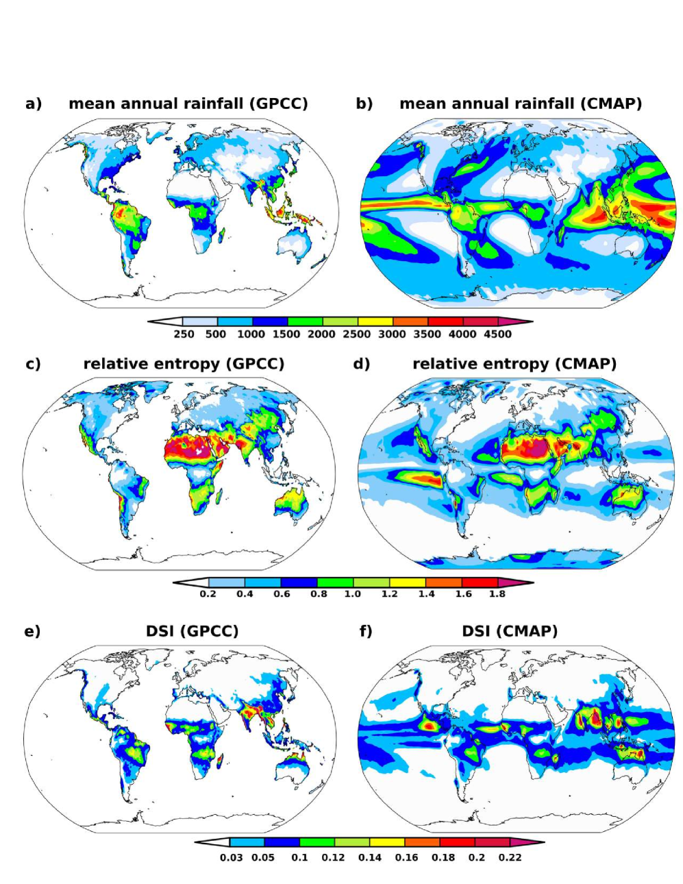
Figure 1: (a, b) Mean annual rainfall $\overline{R}$ (mm yr^-1), (c, d) relative entropy $\overline{D}$ and (e, f) dimensionless seasonality index $\overline{S}$ for the GPCC land dataset (left column) and CMAP dataset (right column).

In Fig. 1 mean annual precipitation, relative entropy and the dimensionless seasonality index for the GPCC land dataset are shown over the period 1950-2010. Values over oceans are shown on the right side of Fig. 1 by using the updated 1979-2009 CMAP dataset (Xie and Arkin, 1997). Regions with the largest $D$ are those placed in the subtropical zone between $10^{\circ}$ and $30^{\circ}$ N/S such as subtropical south Africa, eastern Brazil, north Australia, western India, eastern Siberia, eastern Mediterranean sea, the western mountainous regions of America (south-western North America, western Mexico, Andes) and the region between Middle-east and the Hindu Kush-Karakoram mountain ranges. Sub-Saharian Africa, West India and the area in the Pacific Ocean west of Ecuador have the highest global values ($\geq 1.4$). The equatorial regions roughly located between $5^{\circ}$ S and $5^{\circ}$ N, where convective rainfall is almost permanent (Amazon and Congo basins, Indonesian Isles), have values of $D$ less than 0.2. Midlatitude regions as eastern U.S. and northwestern Europe also have low values of relative entropy ($\leq 0.2$) because baroclinic eddies deliver rain fairly constantly throughout the year. Exceptions are the eastern and southern Mediterranean coasts and eastern Pacific, which instead are relatively dry during the boreal summer.

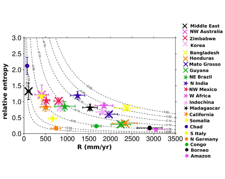
Figure 2: Precipitation-relative entropy diagram for different climatological areas for both GPCC dataset. Overplotted are isolines of dimensionless seasonality index. Error bars denotes the range of inter-annual variability. Monsoonal precipitation regimes typically have $S\geq 0.05$.

In Fig.  1(e) the DSI is shown over land for the GPCC dataset while its patterns over oceans can be seen in Fig. 1(f) from CMAP dataset. Since $R$ and $D$ are generally observed to be negatively correlated, the largest values of $S$ are generally found in regions with intermediate levels of annual rainfall such as northeast region of Brazil, western Africa, northern Australia and western Central America. The DSI is high also in parts of South and Southeast Asia where both the total annual rainfall and RE can be also extremely high (e.g. the Bengal region). Equatorial regions (Indonesia, Congo basin, Amazon) and midlatitudes tend to have low values of $S$ because their relative entropy is very small. Furthermore, although one order of magnitude smaller than typical values of tropical regions, there is appreciable seasonality along the west coast of North America and Southwest U.S., midwest plains, Mediterranean regions, Middle-east, east Siberia and Andes. The precipitation-relative entropy diagram of Fig. 2 provides an example of typical $R$, $D$ and $S$ values averaged over specific high-latitude, subtropical and tropical areas.

It is worth noting, at this point, an interesting coarse graining property of $D$. If we partition the year $Y$ in $N$ parts, we can define $D_{N}=\sum_{1}^{N}p_{j}\log_{2}(Np_{j})$ with $p_{j}=r_{j}/R$ and $r_{j}$ the accumulated precipitation over the $j$th time period $Y/N$ (e.g. $N=12$ for monthly precipitations). In general $D_{N}\neq D_{M}$ for $N\neq M$ so the use of different time bins (e.g. months and pentads) will give different values of relative entropy. However, general properties of the RE allow us to say that if $N\geq M$, then $D_{N}\geq D_{M}$ and $S_{N}\geq S_{M}$ (see Appendix A.3 for a formal proof). This gives us confidence on high-$D$ values, which therefore must be lower than the “true” $D$. This general coarse-graining property is very useful to set lower bounds to values of $D$ and $S$ at any chosen time resolution. In Fig. 3(a) we show $D_{73}-D_{12}$ (pentads minus months) and note that the values of relative entropy obtained from pentad means are slightly larger than those derived from monthly means. The error is less than $0.1$ over most of the global surface, except in the subtropical high regions where it amounts to about $0.2$-$0.4$. Since these areas are very dry, the dimensionless seasonality index $S$ will not be significantly affected (Fig. 3(b)). We note that regions featuring large values of $S$ (e.g. $S\geq 0.05$) have errors $S_{73}-S_{12}$ generally smaller than $5\cdot 10^{-3}$. Since $S$ is almost unaffected by the choice of the time resolution in regions where $S$ is large, as in the global monsoon region (Trenberth et al, 2000; Wang and Ding, 2008), it is a particularly robust index for studying precipitation regimes of monsoonal climates.

3.2 Comparison between land datasets

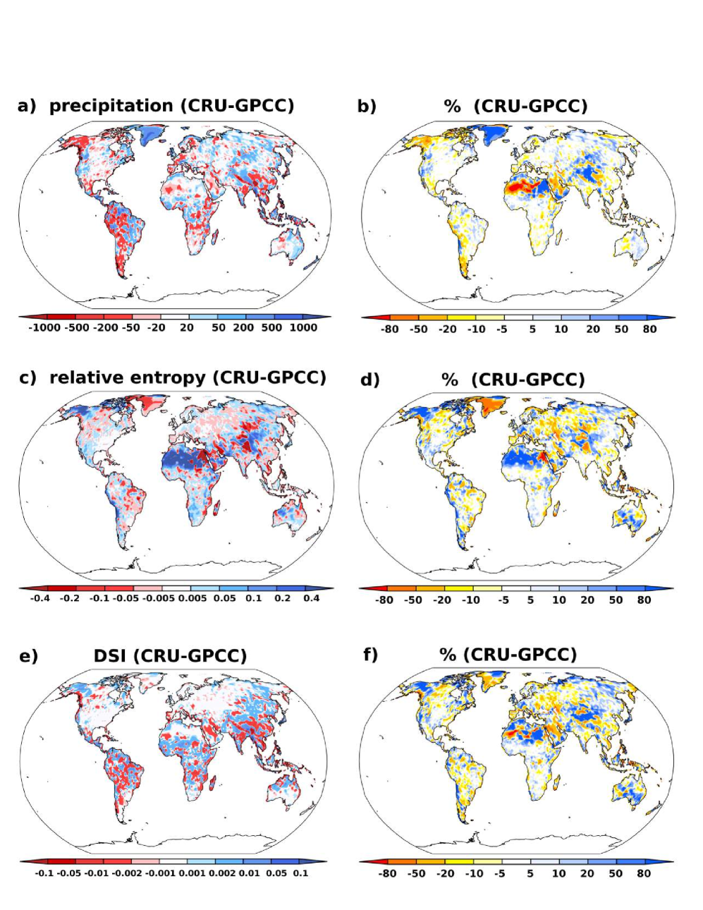
Figure 4: Differences (a, c, e) and relative differences (b, d, f) between the CRU and the GPCC datasets for the same quantities in Fig. 1 over the period 1950-2010.

Differences between the land-based CRU and GPCC datasets are shown in Fig. 4. Inconsistencies of the mean annual precipitation (Fig. 4(a, b)) in the two gridded datasets have already been documented in detail by Schneider et al (2013); instead here we mostly focus on the differences in the rainfall seasonality in terms of $D$ (Fig. 4(c, d)). We note relative differences of $D$ up to $20\%$ in the semiarid or arid regions of Sahara, Middle-East and central Asia and also in areas where the two datasets agree reasonably well in terms of annual total precipitation.

As discussed in Appendix, $D$ is related to the number of wet months. Therefore a difference $D_{\mathrm{cru}}-D_{\mathrm{gpcc}}$ implies a relative difference of the number of wet months $n^{\prime}_{\mathrm{gpcc}}/n^{\prime}_{\mathrm{cru}}\approx 2^{(D_{\mathrm{cru}}-D_{\mathrm{gpcc}})}\approx 0.3$ for $D_{\mathrm{cru}}-D_{\mathrm{gpcc}}=0.4$ and $n^{\prime}_{\mathrm{gpcc}}/n^{\prime}_{\mathrm{cru}}\approx 0.15$ for $D_{\mathrm{cru}}-D_{\mathrm{gpcc}}=0.2$. Considering that in such semiarid regions (e.g. sub-Saharan Sahel) precipitations are concentrated within one-two months, such uncertainties in $D$ reveal fairly large inconsistencies between the two observational datasets in reproducing the time distribution of the precipitation events. On the contrary, in regions such as the slopes of the Himalaya, where there are large differences in the annual total rainfall (up to $1000$ mm/year), differences in relative entropy are relatively small ($\approx 0.05$) and hence the two datasets agree reasonably well in reproducing the monthly precipitation signal. Differences in the DSI between CRU and GPCC are shown in Fig. 4(e, f). The two land datasets show remarkable differences in the seasonality index over southern and central America, most of Africa and south-southeastern Asia. Such inconsistencies in the observational datasets are due to differences in the annual total precipitation in the case of South America, in the relative entropy for sub-Saharan Africa and central Asia, and to both terms in the case of east Indochina and Madagascar.

3.3 The dimensionless seasonality index and the global monsoon regions

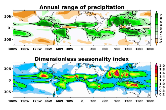
Figure 5: Annual range of precipitation (mm/day) and DSI ($\times 10$) for the CMAP climatology. The global monsoon domain (black thick line) is defined by the annual range equal to $2.5$ mm/day and DSI equal to $0.05$.

The DSI combines information about seasonality and intensity of rainfall and therefore it is a useful indicator of the extent of monsoonal precipitation regions (Wang and Ding, 2008). Rainfall is indeed the most important monsoon variable given the high socioeconomic and ecological impact, and indexes based on rainfall are widely used to study the global monsoon (Wang et al, 2011; Kitoh et al, 2013; Lee and Wang, 2014). In Fig. 5 the DSI is compared to the Annual Range of Precipitation (ARP) (Wang and Ding, 2008; Wang et al, 2011). The ARP is defined as the local summer minus winter precipitation rate, i.e. the MJJAS minus NDJFM precipitation rate in the northern hemisphere and NDJFM minus MJJAS in the southern hemisphere.

Direct comparison of the the two indicators in Fig. 5 shows that regions featuring high DSI capture fairly well the global monsoon region. The global monsoon domain, defined by Wang et al (2011) as the area in which the ARP is greater than $2.5$ mm day^-1, is described also by the isoline $S\approx 0.05$. The two domains match pretty well over land in Africa, Central-South America and Australia although differences are found over the Atlantic and Pacific ocean. Let us note that the DSI is positive definite whereas the ARP has negative values outside the Tropics, where midlatitude precipitations occur during the local winter. While differences between the two criteria appear to be minor, they may still be relevant for assessing the robustness of future changes of the global monsoon domain (Kitoh et al, 2013; Lee and Wang, 2014). Shifts of the borders of the monsoons domain may be especially critical for areas located at the border of monsoonal circulation, as for example the Indus basin (e.g. Hasson et al, 2014) or the arid North America Southwest (Cook and Seager, 2013). These areas might go through critical changes in their precipitation regimes if the extent of the rainfall associated with the monsoonal circulation shifts aways or it is delayed (Seth et al, 2013). Kitoh et al (2013) show that under RCP8.5 scenarios the global monsoon areas as defined by the ARP is mostly unaffected, with little changes over central and eastern tropical Pacific, eastern Asia and southern Indian ocean. Given the small entity of such changes, we stress here the importance of different and alternative monsoon indexes to assess the robustness of future changes in monsoonal precipitation and give more confidence to results on changes of the global monsoon.

4 Comparison with CMIP5 coupled climate models

In this section we evaluate the mean total annual precipitation and the relative entropy for the GCMs listed in Table 1 and compare it with the same indicators estimated for observational datasets. The aim is to assess models’ skill in reproducing the rainfall seasonality as defined by $D$ and show the use of RE maps to determine areas of interest that need more detailed analyses of seasonality using more traditional methods.

4.1 Annual precipitation and relative entropy

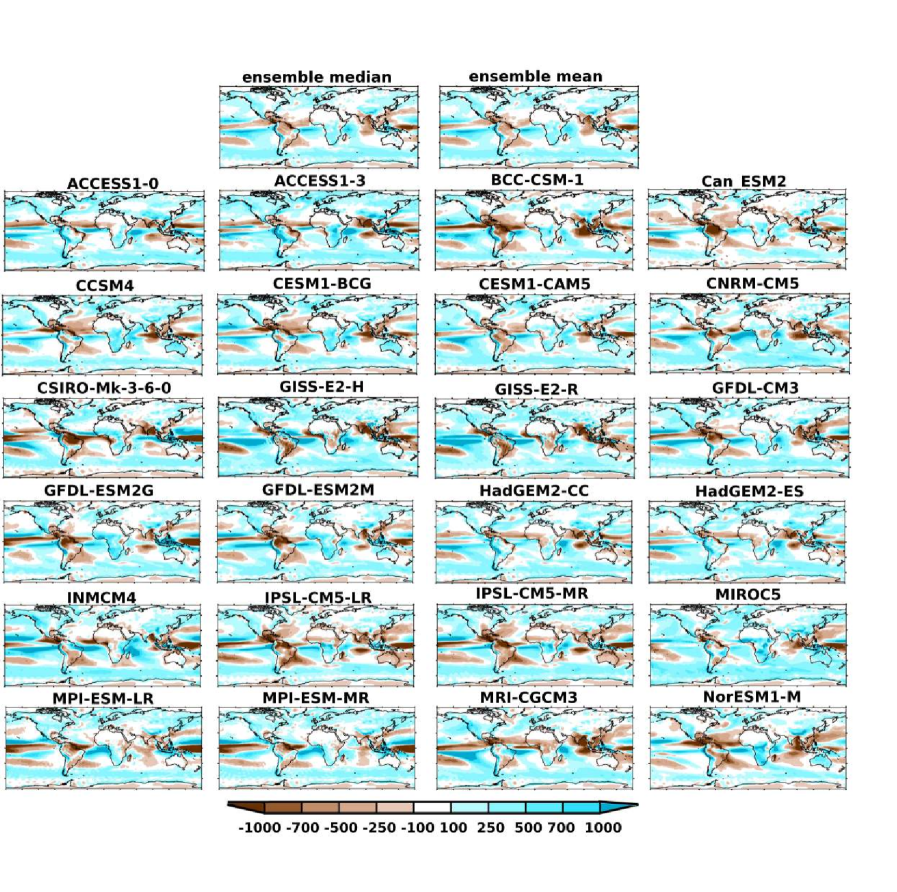
Figure 6: Biases of the CMIP5 models mean precipitation (mm) over the period 1979-2009 relative to the CMAP climatology. The multimodel ensemble median and mean are also shown.

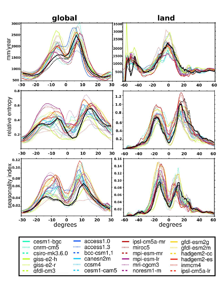
Figure 7: Left column: zonal means of precipitation, relative entropy and dimensionless seasonality index over the whole globe (GPCP and CMAP observation dataset are denoted with black continuous and dashed line respectively) for the period 1979-2008. Right column: as before but over land only (GPCC and CRU are denoted with black continuous and dashed line respectively).

Mean annual rainfall differences between the CMIP5 models listed in Table 1 and CMAP observations are shown in Fig. 6. It is noted that the double ITCZ problem (Lin, 2007) – the additional band of precipitation south of the equator in the Pacific ocean – affects most of the CMIP5 models and it is particularly strong in those with low resolution such as the GISS models or the INMCM4. The double ITCZ bias is one of the most persisting GCMs bias and there has been little improvement from CMIP3 to CMIP5 models (Hwang and Frierson, 2013a). In CMIP5 models it improves as the model resolution increases (MIROC5), although it persists also in models with high horizontal resolution (MRI-CGCM3). The zonal mean of the global precipitation field (Fig. 7) shows the excess of rainfall due to the double ITCZ. In Fig. 7 it can also be seen that models generally show a large spread in the latitudinal position of the maxima of zonal mean of precipitation. These problems may be directly related to how models simulate the ocean meridional heat transport (Frierson et al, 2013). The ITCZ problems seems therefore to be constrained by the surface heat fluxes and thus related to the capability of models to correctly simulate clouds and other controls of the surface solar energy flux (Hwang and Frierson, 2013a).

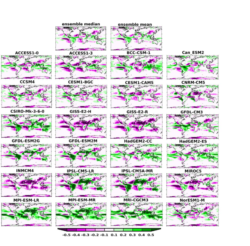
Figure 8: As in Fig. 6, but for relative entropy.

Overall, CMIP5 models tend to have a too large RE over tropical Latin America and a too small RE over Western Africa, Western Mexico and East Asia. This is evident from the multimodel ensemble mean MME and median MMM (Fig. 8). Most of models reproduce fairly well the RE pattern over Southern Africa, with negative biases exhibited only by few models (BCC-CSM-1, GISS-E2-R, GISS-E2-H). The MME and MMM feature small biases also over Australia, due to the cancellation of large positive (e.g. IPSL-CM5-LR) or negative (e.g. GISS-E2-R) biases shown by single models. A large negative RE bias over East Asia, extending from north-eastern China up to the Tibetan region, is present in all models and it is particularly severe in some GCMs (up to $-0.5$, e.g. in GISS-E2-R). The inmcm4 and the GISS models have a general tendency to underestimate RE over both land and oceans, whereas the MRI-CGCM3 and MPI-ESM models tend to overestimate RE.

Zonal means (Fig. 7) reveal that models generally perform better over land. However they show a large dry bias in the precipitation at around $20^{\circ}$ N associated with the South Asian Monsoon (Turner and Annamalai, 2012; Sperber et al, 2013; Hasson et al, 2013, 2014; Boos and Hurley, 2013) over the Indian region (e.g. HadGEM2, Fig. 6). Central America and northern South America also feature strong negative rainfall biases (Hwang and Frierson, 2013b). MPI-ESM-LR largely overestimates the RE in the Southern Hemisphere, although it behaves fairly realistically in the Northern one (Fig. 7). In the equatorial zone ($10^{\circ}$ S-$10^{\circ}$ N) we observe that most of the CMIP5 model feature very large values of RE (for example over the Amazon and eastern Africa region, with GFDL-ESM2G, GFDL-ESM2M or CSIRO-Mk3.6.0 having $D\geq 0.4$, error of order $400\%$) in areas characterized by values of RE typically smaller than 0.2. Exceptions are the GISS-E2-H, GISS-E2-R, MIROC5 and INMCM4 which instead underestimate the RE over the tropics. Overall CESM1-CAM5 model is the best at simulating the observed RE.

Let us note, to conclude this biases analysis, that models errors in RE are not removed by a simple mean bias adjustment of $r_{m}$. Bias adjustment algorithms have been developed to bring GCMs simulations closer to observations before applying statistical and dynamical downscaling (e.g. Christensen et al, 2008; Li et al, 2010). Given the monthly precipitations $r_{m,j}$ (month $m$, year $j$) and the observations $\rho_{m,j}$, a mean bias adjustment would lead to new monthly precipitations $r_{m,j}^{\prime}=\alpha_{j}r_{m,j}$, with $\alpha_{j}=\sum_{m}\rho_{m,j}/\sum_{m}r_{m,j}$ and bias adjusted rainfall fractions $p^{\prime}_{m,j}=$$r^{\prime}_{m,j}/\sum_{m}r^{\prime}_{m,j}=$ $\alpha_{j}r_{m,j}/\sum_{m}\alpha_{j}r_{m,j}=$$p_{m,j}$. Thus, a mean bias adjustment does not affect the monthly precipitation fractions, thus leaving the relative entropy unaltered.

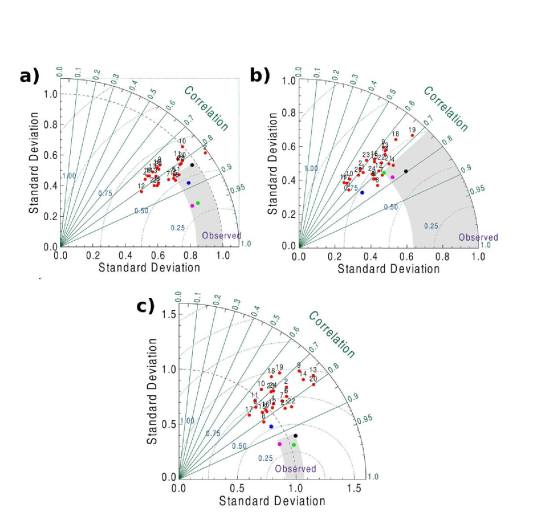
Figure 14: Taylor diagrams for mean annual precipitation (a), relative entropy (b) and seasonality index (c). CMIP5 models are numbered as in Table 1. The MME, CRU, GPCP and CMAP are represented by the blues, black, green and magenta dots respectively. GPCC is taken as reference and standard deviations are normalized with respect to GPCC. The grey shaded areas are indicative of the range of observational uncertainty. The correlation analysis is restricted to land.

Table 1: List of the CMIP5 models used for this study. Numbers are used to identify them in Fig. 14

Number	Model name	Modelling Centre	Country	AGCM resolution (lon$\times$lat)
1	ACCESS1.0	CAWCR ${}^{\textrm{{a}}}$	Australia	192$\times$145/L38
2	ACCESS1.3	CAWCR	Australia	192$\times$145/L38
3	BCC-CSM1.1	BCC ${}^{\textrm{{b}}}$	China	128$\times$64/L26
4	CanESM2	CCCMA ${}^{\textrm{{c}}}$	Canada	128$\times$64/L35
5	CCSM4	NCAR ${}^{\textrm{{d}}}$	USA	288$\times$192/L26
6	CESM1-BGC	NCAR	USA	288$\times$192/L26
7	CESM1-CAM5	NCAR	USA	288$\times$192/L30
8	CNRM-CM5	CNRM/CERFACS ${}^{\textrm{{e}}}$	France	256$\times$128/L31
9	CSIRO-Mk3.6.0	CSIRO/QCCCE ${}^{\textrm{{f}}}$	Australia	192$\times$96/L18
10	GISS-E2-H	GISS ${}^{\textrm{{g}}}$	USA	144$\times$90/L40
11	GISS-E2-R	GISS	USA	144$\times$90/L40
12	GFDL-CM3	GFDL ${}^{\textrm{{h}}}$	USA	144$\times$90/L48
13	GFDL-ESM2G	GFDL	USA	144$\times$90/L24
14	GFDL-ESM2M	GFDL	USA	144$\times$90/L24
15	HadGEM2-CC	MOHC ${}^{\textrm{{i}}}$	UK	192$\times$145/L60
16	HadGEM2-ES	MOHC	UK	192$\times$145/L38
17	INMCM4	INM ${}^{\textrm{{j}}}$	Russia	180$\times$120/L21
18	IPSL-CM5A-LR	IPSL ${}^{\textrm{{k}}}$	France	96$\times$95/L39
19	IPSL-CM5A-MR	IPSL	France	96$\times$95/L19
20	MIROC5	MIROC ${}^{\textrm{{l}}}$	Japan	256$\times$128/L40
21	MPI-ESM-MR	MPI-M ${}^{\textrm{{m}}}$	Germany	192$\times$96/L95
22	MPI-ESM-LR	MPI-M	Germany	192$\times$96/L47
23	MRI-CGCM3	MRI ${}^{\textrm{{n}}}$	Japan	$320\times 160$/L48
24	NorESM1-M	NCC ${}^{\textrm{{o}}}$	Norway	144$\times$96/L26
a Centre for Australian Weather and Climate Research; b Beijing Climate Centre, China Meteorological Administration; c Canadian Centre for Climate Modelling and Analysis; d National Center for Atmospheric Research; e Centre National de Recherchers Meteorologiques/Centre Europeen de Recherche et Formation Avancees en Calcul Scientifique; f Commonwealth Scientific and Industrial Research Organization/Queensland Climate Change Centre of Excellence; g NASA Goddard Institute for Space Studies; h NOAA Geophysical Fluid Dynamics Laboratory; i Met Office Hadley Centre; j Institute for Numerical Mathematics; k Institute Pierre-Simon Laplace; l Atmosphere and Ocean Research Institute (The University of Tokyo), National Institute for Environmental Studies, and Japan Agency for Marine-Earth Science and Technology; m Max Planck Institute für Meteorologie; n Meteorological Research Institute ; o Norwegian Climate Centre

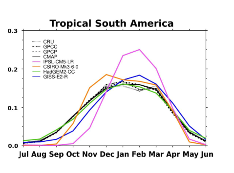
Figure 9: Precipitation frequencies $p_{m}=r_{m}/R$ for observation datasets CRU, GPCC, GPCP, CMAP and four models (CSIRO-Mk3-6-0, IPSL-CM5-LR, HadGEM-CC and GISS-E2-R) over tropical Latin America.

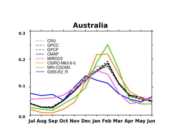
Figure 10: Precipitation fractions $p_{m}=r_{m}/R$ for observation datasets CRU, GPCC, GPCP, CMAP and four models (CSIRO-Mk3-6-0, MRI-CGCM3, MIROC5 and GISS-E2-R) over Australia.

Table 2: Coordinates boundaries (east, south, west, north) of the rectangular areas shown in Fig. 2 (upper part of the table) and Fig. 10-Fig. 9 (lower part of the table).

Area	East	South	West	North
Mato Grosso	$60^{\circ}$ E	$14^{\circ}$ S	$55^{\circ}$ W	$10^{\circ}$ S
NW Australia	$125^{\circ}$ E	$23^{\circ}$ S	$135^{\circ}$ E	$18^{\circ}$ S
N India	$75^{\circ}$ E	$20^{\circ}$ N	$88^{\circ}$ E	$25^{\circ}$ N
NE Brazil	$45^{\circ}$ E	$10^{\circ}$ S	$35^{\circ}$ E	$0^{\circ}$ N
Somalia	$40$ E	$0$ N	$50$ E	$10$ N
NW Mexico	$112$ W	$20$ N	$104$ W	$32$ N
S Italy	$12$ E	$36$ N	$19$ E	$42$ N
Congo	$15$ E	$5$ S	$25$ E	$5$ N
N Germany	$7$ W	$51$ N	$12$ E	$55$ N
Chad	$15$ W	$15$ N	$23$ W	$20$ N
Borneo	$108$ E	$4$ S	$119$ E	$8$ N
Amazon	$70$ W	$5$ S	$65$ W	$5$ N
Indochina	$100$ E	$10$ N	$110$ E	$20$ N
Madagascar	$42$ E	$25$ S	$50$ E	$12$ S
Brazil/Guyana	$65$ W	$3$ S	$55$ W	$3$ N
California	$125$ W	$33$ N	$115$ W	$42$ N
Guinea	$20$ E	$0$ N	$8$ E	$14$ N
Korea	$115$ E	$35$ S	$130$ E	$41$ N
Bangladesh	$88$ E	$22$ S	$92$ E	$26$ N
Zimbabwe	$20$ E	$25$ S	$35$ E	$10$ S
Honduras	$86$ W	$13.5$ N	$84$ W	$15.5$ N
Middle East	$36$ E	$30$ N	$40$ E	$34$ N
Australia	120 E	30 S	150 E	20 S
Sub-Sahara	10 W	15 N	30 E	23 N
West Africa	0 E	5 N	30 E	15 N
Tropical South America	60 W	20 S	40 W	5 S
East Asia	90 E	30 N	120 E	50 S

Table 3: Correlation pattern (PC), root mean square error (RMSE) and standard deviation ($\sigma$) of the observational datasets (GPCC, CRU, GPCP, CMAP) and of the CMIP5 models (Fig. 14). Comparison is made with the GPCC dataset and restricted over land for the 1950-2010 climatology. Values of RMSE and $\sigma$ are normalized with respect to the standard deviation of GPCC $\sigma_{\textrm{gpcc,R}}=807$ mm, $\sigma_{\textrm{gpcc,D}}=0.47$ and $\sigma_{\textrm{gpcc,S}}=0.034$. For observations, bold character highlights values of PC and $\sigma$ defining the observation uncertainty range. Models which are placed within the observation uncertainty range are also highlighted in bold whereas those farthest from the reference (the largest RMSE) are highlighted in bold italics.

number/	model		annual precipitation				relative entropy				DSI
color			PC	RMSE	$\sigma$		PC	RMSE	$\sigma$		PC	RMSE	$\sigma$
reference	GPCC		1	0	$807$ mm		1	0	0.47		1	0	0.034
black	CRU		0.83	0.57	0.97		0.79	0.60	0.74		0.92	0.39	1.07
green	GPCP		0.94	0.32	0.89		0.72	0.69	0.63		0.95	0.31	1.03
magenta	CMAP		0.95	0.32	0.84		0.78	0.63	0.67		0.93	0.35	0.91
1	ACCESS1.0		0.84	0.54	0.87		0.62	0.78	0.57		0.77	0.66	0.97
2	ACCESS1.3		0.82	0.62	1.08		0.59	0.80	0.58		0.74	0.84	1.24
3	BCC-CSM1.1		0.78	0.62	0.75		0.63	0.80	0.44		0.71	0.74	0.92
4	CanESM2		0.76	0.65	0.68		0.73	0.68	0.71		0.76	0.71	1.06
5	CCSM4		0.83	0.55	0.84		0.71	0.71	0.58		0.77	0.76	1.18
6	CESM1-BGC		0.83	0.55	0.84		0.72	0.70	0.58		0.77	0.76	1.18
7	CESM1-CAM5		0.83	0.55	0.79		0.73	0.69	0.63		0.77	0.72	1.13
8	CNRM-CM5		0.83	0.57	0.73		0.76	0.67	0.57		0.81	0.59	0.89
9	CSIRO-Mk3.6.0		0.75	0.66	0.81		0.62	0.80	0.75		0.72	0.98	1.40
10	GISS-E2-H		0.75	0.70	0.99		0.57	0.82	0.49		0.65	0.87	1.10
11	GISS-E2-R		0.78	0.63	0.92		0.54	0.84	0.46		0.67	0.79	0.96
12	GFDL-CM3		0.81	0.62	0.61		0.70	0.71	0.63		0.77	0.68	1.03
13	GFDL-ESM2G		0.75	0.65	0.75		0.64	0.77	0.74		0.77	0.95	1.48
14	GFDL-ESM2M		0.76	0.64	0.71		0.65	0.76	0.73		0.76	0.90	1.39
15	HadGEM2-CC		0.84	0.53	0.82		0.63	0.77	0.66		0.76	0.67	0.93
16	HadGEM2-ES		0.85	0.52	0.83		0.62	0.78	0.67		0.76	0.67	0.97
17	INMCM4		0.80	0.59	0.91		0.57	0.82	0.83		0.71	0.70	0.83
18	IPSL-CM5A-LR		0.75	0.65	0.71		0.64	0.79	0.91		0.64	0.95	1.22
19	IPSL-CM5A-MR		0.75	0.65	0.79		0.68	0.76	0.54		0.66	0.97	1.29
20	MIROC5		0.80	0.61	0.94		0.61	0.79	0.70		0.80	0.87	1.43
21	MPI-ESM-MR		0.82	0.58	0.70		0.70	0.70	0.68		0.81	0.65	1.10
22	MPI-ESM-LR		0.83	0.57	0.72		0.67	0.73	0.64		0.82	0.65	1.10
23	MRI-CGCM3		0.81	0.60	0.92		0.58	0.81	0.60		0.70	0.82	1.10
24	NorESM1-M		0.77	0.64	0.89		0.68	0.73	0.48		0.71	0.82	0.92
blue	MME		0.88	0.47	0.89		0.73	0.72	0.48		0.85	0.52	0.92

4.2 Interpretation of RE biases

In order to clarify the reasons of the RE biases documented in the previous section, we focus on five areas – tropical Latin America, central Australia, Sub-Saharan Africa, Western Africa and East Asia – where either most of the models show consistent biases or some of them feature very large RE biases – and analyze the origin of such biases in terms of precipitation fractions. Coordinates of their rectangular domains are listed in Tab. 2.

Most of models show a consistent positive RE biases over tropical South America (Fig. 8). In Fig. 9 a comparison with observations is shown for some of the most (IPSL-CM5-LR and CSIRO-Mk3-6-0) and least (HadGEM2-CC and GISS-E2-R) biased CMIP5 models. The reason of the RE positive bias is particularly evident from the IPSL simulation, which exaggerates the December-March $p_{m}$ while underestimating them in the pre-monsoonal season. A similar behavior, though less accentuated, is observed also in the CSIRO model. A less severe bias characterizes the GISS model while the HadGEM2-CC captures extremely well the monthly rainfall fractions and presents almost no RE biases over the region.

In Fig. 10 monthly precipitation frequencies $p_{m}$ are shown for observations and four CMIP5 models (MRI-CGCM3, CSIRO-Mk3-6-0, MIROC5 and GISS-E2-R) over the Australian region. The first two models show positive biases in RE whereas the last two models have negative biases. Note that the mean annual rainfall does not show large biases in these regions, so the anomalies in RE must be related only to the monthly distribution of the annual rainfall. Comparison of models and observations reveals a qualitative behavior consistent with our interpretation of $D$, with MRI-CGCM3 and CSIRO-Mk3-6-0 simulating a too dry summer season and a too steep increase in December, resulting in a too short rainy season duration. On the other hand, MIROC5 and GISS-E2-R underestimate the rainfall fractions during January-April and overestimate them during the dry period July-October, resulting in a too flat $p_{m}$ annual distribution and negative biases in RE.

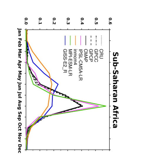
Figure 11: Precipitation fractions for observation datasets CRU, GPCC, GPCP, CMAP and four models (IPSL-CM5A-LR, inmcm4, MPI-ESM-LR and GISS-E2-R) over Sub-Saharan Africa

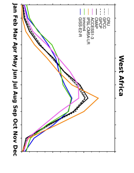
Figure 12: Precipitation fractions for observation datasets CRU, GPCC, GPCP, CMAP and four models (IPSL-CM5A-LR, inmcm4, ACCESS1-3 and GISS-E2-R) over western Africa

Over the semi-arid Sub-Saharan region (Fig. 11), observations show a strong rainfall peak in August ($p_{\mathrm{aug}}\approx 0.4$) related to the marginal influence of the West African monsoon (Vellinga et al, 2013) in the southern part of the region. As shown in Fig. 1, these areas feature the highest RE values ($D\approx 1.6$) in the world. CMIP5 models generally underestimate RE in this region, except a few ones such as the two IPSL-CM5A and MPI-ESM models, which instead have positive biases in northern Africa. A direct inspection of their rainfall fractions reveal that MPI-ESM-LR and IPSL-CM5A-LR simulate a too pronounced precipitation peak in August ($p_{\mathrm{aug}}\approx 0.5$ and $0.55$ respectively). Positive biases are instead associated with an overestimation of $p_{m}$ in late spring and an underestimation in summer. This tendency, which is common to most of CMIP5 GCMs, is evident from the inmcm4 and GISS-E2-R (Fig. 11), which are some of the models with the most severe negative biases ($\approx-0.5$). In the Western African monsoon region, south of the semi-arid Sub-Saharan Africa, negative biases in RE are less severe (Fig. 8). A few models have modest positive RE biases (IPSL-CM5A-LR, IPSL-CM5A-MR, MRI-CGCM3). A focus on this area (Fig. 12) again elucidates the link between RE biases in terms of $p_{m}$. The GISS-E2-R and the inmcm4 models, for example, overestimates $p_{m}$ in the dry season (November-April) and underestimates it during the wet season, resulting in a probability distribution $p_{m}$ more uniform, over the year, than what is observed. As an example we also show the rainfall fractions for a GCM (ACCESS1-3) which instead has almost no RE bias in this region. As expected, the annual $p_{m}$ shape agrees relatively well with observations, apart from a slight shift of rainfall towards the early summer. The IPSL-CM5A-LR model, which tends to overestimate the RE, simulate a too pronounced precipitation peak in August.

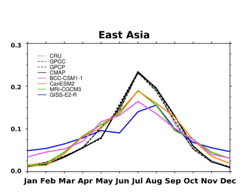
Figure 13: Precipitation frequencies $p_{m}=r_{m}/R$ for observation datasets CRU, GPCC, GPCP, CMAP and four models (BCC-CSM1-1, CanESM2, MRI-CGCM3 and GISS-E2-R) over East Asia.

A persistent, large negative RE bias ($\approx-0.5$), common to all models, is also visible over East Asia in most of the models shown in Fig. 8. Direct inspection of $p_{m}$ shows that models do not capture the right magnitude of the July peak in $p_{m}$ and tend to have a too high rainfall fraction during the dry winter months. This behavior, which remains also in the least biased models (CanESM2 and MRI-CGM3), is particularly evident in models with very large biases such as, for example, GISS-E2-R and BCC-CSM1-1 (Fig. 13). The GISS model, in particular, considerably overestimate the winter rainfall fractions, resulting in a large bias in RE.

The RE can therefore be a very useful metric to test the right shape of the simulated monthly rain frequencies $p_{m}$ and to provide an estimation of the number of wet months. It must be noted however that, from its definition in Eq. 2, the RE is invariant to time translation ($p_{m}\rightarrow p_{m+s}$, with $s=1,\ldots 11$) and therefore not able to provide information about the onset and the decay of the monsoon (Sperber et al, 2013; Hasson et al, 2014), which are other two fundamental aspects of monsoonal regimes. Furthermore, the RE cannot discriminate between regions with two short rainy season and those with a single long one, since, from its own definition, any reshuffle of the $p_{m}$ would not lead to any change in RE.

4.3 Pattern correlation and Taylor diagrams

We conclude our comparison between CMIP5 models and observation by estimating the pattern correlation (PC) and the centered root mean square error (RMSE) between the simulated $R$, $D$, $S$ and the observed ones. The PC and the RMSE are statistics generally used to quantity pattern similarity between two climatic fields ($f$, $r$) defined at $N$ points. They are defined as (Taylor, 2001) $PC=[\sum(f_{n}-\overline{f})(r_{n}-\overline{r})]/(N\sigma_{f}\sigma_{r})$ and $RMSE=\{\sum[(f_{n}-\overline{f})-(r_{n}-\overline{r})]^{2}/N\}^{1/2}$, where ($\overline{f}$, $\overline{r}$) and $\sigma_{f,r}$ are the mean values and standard deviations of $f$ and $r$ respectively and are related through the following relationship: $RMSE^{2}=\sigma_{f}^{2}+\sigma_{r}^{2}-2\sigma_{f}\sigma_{r}PC$. It has to be noted that since the means are subtracted, the PC and the RMSE cannot inform about overall biases (which have been analyzes in the previous sections instead) but just on the centered pattern error. Since the GPCP and CMAP datasets are not bias-adjusted over oceans, we restrict this comparison over land. The GPCC land dataset is taken as a reference and compared to CMIP5 models.

The values of the RMSE and PC for each of the CMIP5 models of Table 1 and the other precipitation gridded datasets are reported in Table 3 and shown through Taylor diagrams (Taylor, 2001) in Fig. 14. Other observational datasets (CRU, GPCP, CMAP) are also compared to GPCC and shown on the same diagrams in order to have an indication about observational uncertainty. In fact, given the problems in accurately measuring a highly spatially and temporally variable field such as precipitation, observational estimates are generally affected by uncertainty and more observational datasets are needed to provide information about the range of such uncertainty. To check if the differences in model performances shown in Figure 14 are significant, we considered, for a few models, all the five ensemble members available on the CMIP platform and obtained by initiating the simulations from different initial conditions. It is found that the ensemble spread is very small and comparable with the size of the dots.

In particular GPCP and CMAP are the closest to GPCC; this is not surprising since these two satellite-based datasets use the GPCC dataset as their rain gauge component over land. We define the range of observational uncertainty in terms of PC such as $[PC_{\mathrm{low}},1]$ and in term of $\sigma$ such as $[\sigma_{\mathrm{low}},\sigma_{\mathrm{high}}]$ where $PC_{\mathrm{low}}$ is the lowest PC among the other observational datasets, $\sigma_{\mathrm{low}}=\inf\{\sigma_{\mathrm{gpcc}},\sigma_{\mathrm{obs}}\}$ and $\sigma_{\mathrm{high}}=\sup\{\sigma_{\mathrm{gpcc}},\sigma_{\mathrm{obs}}\}$. We have that $PC_{\mathrm{low}}=0.83$, $[\sigma_{\mathrm{low}}\sigma_{\mathrm{high}}]=[0.84,1]\sigma_{\mathrm{gpcc}}$ for mean annual precipitation; $PC_{\mathrm{low}}=0.72$, $[\sigma_{\mathrm{low}},\sigma_{\mathrm{high}}]=[0.63,1]\sigma_{\mathrm{gpcc}}$ for the RE; $PC_{\mathrm{low}}=0.92$, $[\sigma_{\mathrm{low}},\sigma_{\mathrm{high}}]=[0.91,1.07]\sigma_{\mathrm{gpcc}}$ for the DSI (Fig. 14 and Table 3). A model therefore performs consistently with observations if its $PC>PC_{\mathrm{low}}$ and its $\sigma$ lies within the range $[\sigma_{\mathrm{low}},\sigma_{\mathrm{high}}]$. Models that perform worst are those with $PC\ll PC_{\mathrm{low}}$, a standard deviation $\sigma$ outside the range $[\sigma_{\mathrm{low}},\sigma_{\mathrm{high}}]$.

In terms of precipitation, we note that most of the models are placed outside the observational uncertainty range except ACCESS1-0, CCSM4 and CESM1-BGC (Table 1). While the MME does not necessarily have to outperform every single model (e.g. Sperber et al, 2013), here this is the case ($PC=0.88$, $\sigma=0.89\sigma_{\mathrm{gpcc}}$) and it is consistent with the observations. HadGEM2-ES, HadGEM2-CC and CESM1-CAM5 also perform well with a PC larger or equal than $0.83$ but with a value of the standard deviation just below $\sigma_{\mathrm{low}}=0.84\sigma_{\mathrm{gpcc}}$. Overall, other GCMs are placed not far from the lower bound of the PC ($\approx 0.8$), but some of them underestimate $\sigma$ by a factor $0.3$ or more (e.g. GFDL-CM3, GFDL-ESM2M, IPSL-CM5A-LR), well below $\sigma_{\mathrm{low}}=0.83\sigma_{\mathrm{gpcc}}$, resulting in large RMSE (CanESM2, GFDL-ESM2G, IPSL-CM5-LR). As far as RE is concerned, observational uncertainty is generally larger ($PC_{\mathrm{low}}=0.72$, $\sigma_{\mathrm{low}}=0.63\sigma_{\mathrm{gpcc}}$). This is consistent with the large differences between the CRU and GPCC datasets shown in Fig. 4. CanESM2 ($PC=0.73$, $\sigma=0.71$) and CESM1-CAM5 ($PC=0.73$, $\sigma=0.63$) are within the observational range range whereas CNRMS-CM5 is just slightly outside ($PC=0.57$). Contrary to the case of precipitation, the MME for the RE lies outside such range and does not outperform every single model. Some of the CMIP5 models perform particularly badly and feature a considerably lower PC and $\sigma$, resulting in RMSE almost comparable with $\sigma$ (GISS-E2-H, GISS-E2-R, MRI-CGM3). Again, most of the model are not far from the lower bounds of observational uncertainty. It is interesting to note that the best performing models in terms of the field of mean annual precipitation are not the best in terms of RE. Finally we note that no model is consistent with observations in terms of the DSI, as evident from Fig. 14. This may be due to the fact that the DSI is a diagnostic metrics more complex than precipitation and RE alone – it combines them together, providing integrated information about the intensity of the annual rainfall and the shape of the monthly rain frequency – and therefore it is more unlikely for models to capture equally well spatial variability of both precipitation and RE. Rainfall is a complex field and it is challenging for models to properly simulate it. Lack of model agreement between mean precipitation and other, more complex aspects are found also, for example, when comparing total precipitation and upper quantiles of the precipitation distribution. For example, analyzing CMIP5 models, Mehran et al (2014) show that models best simulating the total precipitation amounts not necessarily are also the best performing in precipitation upper quantiles.

The MME outperforms every single model but still lies outside the observational range. When all three metrics are considered, CESM1-CAM5 is overall one of best model in terms of spatial variability and magnitude (as evident from Fig. 8–Fig. 7) whereas the worst performing models are GISS-E2-H and GISS-E2-R.

5 Conclusions

Future improvements and developments of the GCM representation of precipitations strongly rely on rigorous metrics for their validation (e.g. Mehran et al, 2014). Accurate, reliable diagnostics of rainfall seasonality is a necessary tool for gauging GCMs performance, evaluating their realism and quantifying changes in the hydroclimatic regimes. In this study we used novel measures of rainfall seasonality (Feng et al, 2013) based on information entropy, namely the relative entropy (RE) and the dimensionless seasonality index (DSI), for characterizing the seasonality of precipitation regimes during the 1950-2010 period over lands and oceans using the four recently updated precipitation gridded datasets GPCC, CRU, CMAP, GPCP (Fig. 1 and Fig. 2) and for assessing CMIP5 models’ ability capture the observed patterns of RE and DSI.

The RE provides an integral measure of the seasonality of the annual rainfall curve whereas the DSI quantifies the intensity of the rainfall during the wet season. The RE is related to the number of the wet time accumulation bins $n^{\prime}$ through the simple relation $n^{\prime}\approx N\cdot 2^{-D}$, where $N$ is the number of temporal accumulation bins in a year. Areas with high RE are therefore characterized by prolonged dry periods and rainfall concentrated in a short time period. Given its own definition, the RE cannot discriminate between unimodal and bimodal rainfall regimes and therefore it does not automatically provide a measure of the duration of the wet season. However, for precipitation regimes known to be unimodal (e.g. in the South Asian monsoon region), $n^{\prime}$ coincides with the duration of the wet season and it can be used as a further measure along with more tradition ones such as the monsoon retreat and onset time.

It is found that Equatorial (Indonesia, Congo basin, Amazon) and midlatitude regions have low values of the DSI because, in spite of the large mean annual precipitation, their relative entropy is very small ($\leq 0.05$). Arid and semiarid regions around $20^{\circ}$ N with intermittent precipitation regimes – like the sub-Saharan Sahel – are characterized by large RE and feature very low DSI because of the very little annual precipitation. Highest DSI ($\geq 0.05$) are therefore found in those regions with intermediate-to-high levels of mean annual rainfall and RE such as northeast region of Brazil, Western Africa, Northern Australia, Western Mexico and South-Southeast and Eastern Asia, which constitute the so-called global monsoon region (Wang and Ding, 2008). According to the DSI, the west coast of North America, Mediterranean, Middle-East regions and the Andes also feature appreciable seasonality, since rainfall in these regions is confined to the (local) winter months.

The RE and DSI have two practical advantageous features: a) the robustness against changes of the accumulation temporal bin of the precipitation time series and b) the coarse-graining properties of the RE (Fig. 3). The first property guarantees a quantification of seasonality which is as much as possible independent of the time bin (day, pentad, week, month) used to accumulate precipitation. The second property allows us to establish lower bounds for the RE and DSI with respect to values which would be obtained from higher-resolution data, which are not always available.

Comparison of simulations performed with 24 CMIP5 coupled atmosphere-ocean general circulation models with the precipitation datasets over the period 1950-2010 reveals consistent positive (South America) and negative (East Asia, northern Africa) RE biases across models (Fig. 10). Such biases are related to GCMs’ inability to simulate the right monthly fractions of rainfall along the year. The GCMs’ negative RE bias over western Africa is due to a positive precipitation bias in the West African monsoon region in late spring and a negative precipitation bias during July-September (Fig. 11 and  12). A similarly consistent picture has been shown to explain also the large negative bias in east Asia, related to rainfall fractions which are too low during the wet May-September period and too large during the dry October-April period, thus resulting in a $p_{m}$ sequence not peaked enough (Fig. 13). On the other hand, the positive RE bias over tropical southern American (Fig. 9) is due to the opposite tendency to overestimate the monthly rainfall fractions during the local summer and underestimate them in the late spring/early summer period, resulting in an excessively peaked $p_{m}$. The presence of these RE biases consistently across the evaluated CMIP5 GCMs indicate the presence of general deficiencies in the models in simulating tropical precipitation and, in particular, monsoons (Turner and Annamalai, 2012). These systematic RE errors appear to be not very sensitive to differences in model horizontal resolution since they are found in models with higher and lower space resolution and are likely to be due general shortcomings in representing the dynamics or physics of climatic phenomena.

In terms of spatial variability, pattern correlation analysis over continents clearly shows that CMIP5 models have a better skill in reproducing the variability pattern of precipitation compared to RE (Fig. 14) with few models consistent with observations. In particular, no model reproduces the DSI spatial variability consistently with observations. Overall, CESM1-CAM5 is one of the best performing models for all three metrics, whereas the worst performing are GISS-E2-H and GISS-E2-R.

It has to be noted that RE and DSI do not provide a complete description of rainfall seasonality since they do not take into account the timing of the wet season. Their main scope is to provide an easy way to compare maps of RE/DSI between various datasets to determine areas of interest, and then to undertake a more detailed analysis of seasonality in these regions using more traditional measures of seasonality as we have shown for the West African, the Australian, the southern American and the eastern Asian regions.

The methodology underlying the definition of the RE and DSI is very general and applicable to much more general cases than what shown in this study. In principle it may be adapted to other periodic or quasi-periodic climatic sequences of positive-definite variables. Such tools seems therefore very promising for assessing models’ capability to simulate spatial and temporal patterns of the rainfall diurnal cycle, which is the primary mode of variability in the equatorial regions, where heavy rains are concentrated in the afternoon hours. Furthermore, the diagnostic tools presented in this study can be used for studying changes in rainfall seasonality for future climate projections under anthropogenic forcing in addition to more traditional approaches (Huang et al, 2013; Wang et al, 2011; Lee and Wang, 2014). Future efforts in this direction will focus therefore on the application to the rainfall diurnal cycle and on the analysis of 21st century greenhouse-forced climate projections.

Appendix A Properties of the relative entropy

A.1 Relative entropy and information entropy

Given a discrete probability distribution $p=\{p_{m}\}_{m=1}^{N}$ describing a random variable, the information entropy associated with ${p_{m}}$ is a measure of the uncertainty of a random variable described by $p$ and it is defined as

$$\mathcal{H}\left(p\right)\equiv-\sum_{m}^{N}p_{m}\log_{2}p_{m}$$ (4)

and $0\leq\mathcal{H}\leq\max(\mathcal{H})$, where $\max(\mathcal{H})=\log_{2}N$ for the uniform distribution $p_{m}=1/N$ (maximum uncertainty) and 0 if one out of the $N$ values of $p$ is equal to one and all the remaining are zero ($x\log x\rightarrow 0$ as $x\rightarrow 0$)(no uncertainty). In the case considered in this study, $N=12$ and $\max(\mathcal{H})=\log_{2}12$. The relative entropy of $p$ with respect to $q$, $\mathcal{D}(p|q)$, is introduced instead to measure how different two probability distribution $\{p_{m}\}_{m=1}^{N}$ and $\{q_{m}\}_{m=1}^{N}$ are:

$$\mathcal{D}(p|q)\equiv\sum_{m=1}^{N}p_{m}\log_{2}\left(\frac{p_{m}}{q_{m}}\right)$$ (5)

and it measures the inefficiency of assuming $q$ when instead the true distribution is $p$. It can be demonstrated (Cover and Thomas, 1991) that $\mathcal{D}(p|q)\geq 0$ for any $p,q$ and $\mathcal{D}(p|q)=0$ if and only if the two probability distributions are the same. The relative entropy is not symmetric, $\mathcal{D}(p|q)\neq\mathcal{D}(q|p)$ and therefore is not a distance in a mathematical sense. However it is still useful to think of it as a distance between probability distributions. For defining the seasonality index we define $D\left(p\right)$ such as

$$D(p)\equiv\sum_{m=1}^{N}p_{m}\log_{2}\left(N\,p_{m}\right)$$ (6)

that is such as the relative entropy of the probability distribution $p_{m}$ with respect to the uniform distribution $q_{m}=1/N$, which is taken as a reference. In the following and in the rest of this manuscript we will still refer to $D(p)$ as relative entropy. From this definition it follows that

$$D\left(p\right)=-\mathcal{H}\left(p\right)+\log_{2}N.$$ (7)

As a consequence, for two probability distributions $p$ and $w$, $D\left(p\right)-D(w)=\mathcal{H}(w)-\mathcal{H}\left(p\right)$.

A.2 Relative entropy and the spread of $p_{m}$

Let us assume now that $\{p_{m}\}_{1}^{N}$ are the monthly precipitation fractions ($N=12$). From what said so far, it is expected that the larger it is $D$, the less uniformly the precipitation is distributed throughout the year. So $D$ is related to the “spread” of precipitation signal. This concept can be framed in a rigorous way in information theory by defining the effective number of values of $p$

$$n^{\prime}\left(p\right)=2^{\mathcal{H}\left(p\right)}=12\,\cdot 2^{-D}.$$ (8)

Mathematically $n^{\prime}$ defines the number of months over which $p_{m}$ is considerably different from zero, i.e. the support of $p_{m}$ (Cover and Thomas, 1991). Therefore $n^{\prime}$ can be interpreted as the effective number of wet months in a year. Areas characterized by $D=0$ have $n^{\prime}=12$, that is no significant dry period (non-seasonal rainfall regime), whereas regions featuring $D=D_{\mathrm{max}}=\log_{2}12$, $p_{k}=1$ have their annual precipitation all concentrated in one month (extreme seasonal rainfall regime). For regions having a unimodal seasonal rainfall distribution, $n^{\prime}$ provides a measure of the duration of the wet season (e.g. Indian region). It has to be noted however that different measures of the wet season duration which are not based on integral properties of the rainfall distribution but on local properties – e.g. retreat minus onset dates (Sperber et al, 2013; Kitoh et al, 2013; Hasson et al, 2014), where onset and retreat are defined by the $5$ mm day^-1 threshold – may give different results.

Within this framework, let us also introduce another useful statistical indicator of rainfall seasonality, the centroid. By using circular statistics (Fisher et al, 1993), the first moment of $p_{m}$ (centroid) is defined as

$$C=\textrm{arg}(z),\quad z=\sum_{m=1}^{12}p_{m}e^{i\frac{2\pi m}{12}}$$ (9)

and it is shown in Fig. 15. The centroid provides a measure of the the timing of the wet season. While it can be mathematically defined for any precipitation sequence $r_{m}$ and so in any location, it is really meaningful only for those rainfall regimes that are somewhat “localized” during the year – i.e. having a clear dry and wet period. A more extensive analysis of $C$ in present condition and future emission scenarios will be reported elsewhere.

A.3 Coarse graining properties of $D$

A remarkable property of $D$ is the possibility to control its magnitude as the time resolution of the time series is coarse grained. The choice of a certain time series resolution is somewhat arbitrary and dependent on the data available. It is therefore desirable to have indicators that are stable against changes in the accumulation time bin or, at least, that vary in a controllable way. Relative entropy allows us to set lower bounds for the error associated with the loss of information due to time coarse-graining. If $D_{N}$ is the relative entropy estimated from rainfall data at high time resolution $\tilde{p}_{j}$ (e.g. daily, $N=365$ or pentads, $N=73$), we can aggregate sequentially $\nu$ of the $\tilde{p}_{j}$ (e.g. $\nu=5$ for pentads) and obtain

$$p_{i}=\sum_{j=\nu i-\nu+1}^{\nu i}\tilde{p}_{j}$$ (10)

with $i=1,\ldots M$ and $M=N/\nu$. By using the log sum inequality (Cover and Thomas, 1991)

$$\sum_{i=1}^{n}a_{i}\log{\frac{a_{i}}{b_{i}}}\geq\left(\sum_{i=1}^{n}a_{i}\right)\log{\frac{\sum_{i=1}^{n}a_{i}}{\sum_{i=1}^{n}b_{i}}},\quad a_{i},b_{i}\geq 0$$ (11)

where the equality holds only if the $a_{i}$ and the $b_{i}$ do not depend on $i$, and from the definition (6) it follows that

$$\sum_{j=1}^{N}\tilde{p}_{j}\log_{2}{\frac{\tilde{p}_{j}}{\tilde{q}_{j}}}\geq\sum_{i=1}^{N/\nu}\left(\sum_{j=\nu i-\nu+1}^{\nu i}\tilde{p}_{j}\right)\left(\log_{2}\frac{\sum_{j=\nu i-\nu+1}^{\nu i}\tilde{p}_{j}}{\sum_{j=\nu i-\nu+1}^{\nu i}\tilde{q}_{j}}\right)=\sum_{i=1}^{M}p_{i}\log_{2}(p_{i}/q_{i})$$ (12)

and therefore

$$D_{N}\geq D_{M}\quad\textrm{for}\quad N\geq M.$$ (13)

From the definition of the dimensionless seasonality index $S$ in Sect. 2 (Equation 3), it is obvious that also $S_{N}\geq S_{M}$ and so information about rainfall seasonality is lost in the upscaling procedure unless the values in each temporal bin are equal. In Fig. 3 the differences $D_{73}-D_{12}$ and $S_{73}-S_{12}$ are shown as an example.

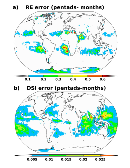
Figure 3: Difference between the RE (a) and the DSI (b) estimated from pentad and monthly means.

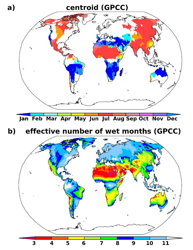
Figure 15: Centroid (a) and effective number of wet months (b) of the monthly precipitation sequence $p_{m}$ for the GPCC dataset. In (a) numbers denotes the months of the year around which $p_{m}$ is centered and in (b) the length in months. The centroid is not shown for regions with $D\geq 0.2$ – corresponding approximately to $n^{\prime}$ greater than $11$.