Parametrization of completeness in symbolic abstraction of bounded input linear systems

Abstract

A good state-time quantized symbolic abstraction of an already input quantized control system would satisfy three conditions: proximity, soundness and completeness. Extant approaches for symbolic abstraction of unstable systems limit to satisfying proximity and soundness but not completeness. Instability of systems is an impediment to constructing fully complete state-time quantized symbolic models for bounded and quantized input unstable systems, even using supervisory feedback. Therefore, in this paper we come up with a way of parametrization of completeness of the symbolic model through the quintessential notion of “Trimmed-Input Approximate Bisimulation” which is introduced in the paper. The amount of completeness is specified by a parameter called “trimming” of the set of input trajectories. We subsequently discuss a procedure of constructing state-time quantized symbolic models which are near-complete in addition to being sound and proximate with respect to the time quantized models.

1 Introduction

Finite symbolic abstractions of control systems are used in algorithmic controller synthesis [7, 8, 9]. Since digital implementations of continuous control systems [4] have quantized and bounded input space, we consider the setting of bounded and quantized-input control systems. For such systems, a state-time quantized abstraction restricted to a compact region gives a finite abstraction, because the set of input trajectories is already finite (quantized and bounded) [11]. The problem of constructing approximately similar state-time quantized symbolic abstraction of possibly unstable quantized-input control systems under stabilizability assumptions has been solved previously [11]. On the other hand, the problem of constructing approximately bisimilar symbolic abstractions of bounded input unstable systems has not been tackled yet. The difference between an approximately bisimilar and an approximately similar abstraction is in the completeness of the abstractions, as explained in the following. An ideal state-time quantized symbolic abstraction of a control system would be exactly bisimilar to the time-quantized system model, but such exactly bisimilar abstraction is almost impossible to realize because of symbolic approximations resulting from quantization of state space. An exact bisimulation relationship between a time quantized system model and a state-time quantized symbolic model can be equivalently factored into the conjunction of the following three conditions, which we call zero deviation, soundness and completeness respectively.

1. Zero deviation: The deviation between the output of a system state and the related symbolic state would ideally be zero.

2. Soundness: Let $s$ be a state of a time-quantized model, and $s_{r}$ be its related symbolic state in the state-time quantized model. Soundness holds if whenever $s_{r}$ transitions to $s_{r}^{\prime}$ by some input, then there is a corresponding input by which $s$ transitions to $s^{\prime}$ which is symbolically related to $s_{r}^{\prime}$. The difference between soundness and an exact simulation  relation is that soundness does not require the outputs of related states to be the same, but for an exact simulation relation to hold, it is necessary (not sufficient) that the outputs of related states are same.

3. Completeness: Completeness is the converse of soundness and is defined as follows. Let $s$ be a state of a time-quantized model, and $s_{r}$ be its related symbolic state in the state-time quantized model. Completeness holds if whenever $s$ transitions to $s^{\prime}$ by some input, then $s_{r}$ transitions to $s_{r}^{\prime}$ by a corresponding input such that $s^{\prime}$ is symbolically related $s_{r}^{\prime}$. Completeness also does not require the outputs of related states to be same, unlike an exact simulation${}^{\ref{foot:milner}}$ relation.

Unlike bisimulation, an exact simulation${}^{\ref{foot:milner}}$ of a state-time quantized model by the time-quantized model only entails zero deviation plus soundness, but not completeness. On the other hand, an exact bisimulation relation between a state-time quantized model and the time-quantized model entails completeness, soundness and zero deviation. The soundness condition ensures that every control law synthesized from the symbolic model has its corresponding control law in the time-quantized system model. The completeness condition ensures that all control laws present in the time-quantized system model have corresponding control laws in the state-time quantized symbolic model; which means that we do not miss out any control laws of the time-quantized system model from the symbolic model while doing controller synthesis on symbolic model. The zero deviation condition ensures that there is no error in the output of the synthesized control law from symbolic model when compared with the actual output of the system for the same control law.

The soundness condition is indispensable because without it the control laws synthesized from the symbolic model would not be correct for the actual system model. But unlike the soundness condition, the zero deviation and completeness conditions are not very imperative. In fact, satisfying the zero deviation condition is very difficult if not impossible because of state-quantization induced symbolic approximations. So in approximately similar symbolic abstraction [9, 13, 12, 11], the zero deviation condition is relaxed as:

Parametrized deviation: There is a parameter specifying an upper bound on the deviation between the states of the system model and related states of the symbolic model. We will call this parameter as proximity.

The extant methodology of approximately similar symbolic abstraction (discussed in [9, 13, 12, 11]) establishes soundness between symbolic model and system model while also specifying the proximity parameter, which is the precision bound of the approximate simulation relation [9, 13, 12, 11]. Parametrization of the amount of deviation (proximity) between a system model and its symbolic model in addition to demonstrating soundness of the model is the advantage of approximately similar symbolic abstraction. Also, a good methodology of symbolic abstraction allows for adjusting the proximity to a very small amount. In this regard, the methodologies discussed in [9, 13, 12, 11] permit sound symbolic abstraction with arbitrarily small proximity. However, a stronger method of abstraction, discussed in [9], can construct an approximately bisimilar (not just similar) finite symbolic model to a time-quantized system model of a globally asymptotically stable system, in which case the abstraction is complete in addition to being sound and proximate.

Although proximity has been parametrized through the notion of approximate simulation [9, 13, 12, 11], no attempt has been made until now to parametrize completeness. Parametrization of completeness would be useful while abstracting bounded input unstable systems that, in many cases, can not have fully complete (plus sound) state-time quantized symbolic models. A parameter for completeness quantifies how exhaustively we can search for control laws using the symbolic model. Our paper is concerned about parametrization of completeness and finding a way of near-complete, sound, and proximate state-time quantized abstraction of bounded and quantized input possibly unstable but locally asymptotically stabilizable linear control systems. We formalize near completeness, soundness and proximity by the notion of trimmed input approximate bisimulation, which is introduced in our paper. We employ supervisory feedback in the process of abstraction. Note that when the input space is bounded, then locally stabilizable divergent linear systems are still not globally asymptotically stabilizable (refer to Subsection 4.3 and Appendix). Therefore we make the distinction between local asymptotic stabilizability and global asymptotic stabilizability of bounded input linear systems. Before we explain our work, we would like to motivate it by discussing some Related Work as follows.

Related Work

For globally asymptotically stable (GAS) continuous control systems, finite approximately bisimilar symbolic automata models with arbitrarily small approximation can be constructed by the procedure discussed in [9]. As such, soundness, completeness and proximity conditions are met by the symbolic model of a GAS system constructed by the procedure discussed in [9]. Regarding unstable systems and also those systems that meet a stabilizing condition [12, 11] but are possibly unstable, there has been work on abstracting the systems into similar symbolic models i.e. based on approximate simulation, but not on approximate bisimulation  [13, 12, 11]. In other words, these approaches [13, 12, 11] for abstracting unstable systems meet the proximity and soundness conditions, but not the completeness condition.

Since global asymptotic stability (GAS) seems crucial for complete symbolic abstraction of control systems, it is tempting to use feedback to globally asymptotically stabilize the system. An idea of globally asymptotically stabilizing the system for symbolic abstraction is discussed in [11]. But the approach in [11] has the following discrepancies:

• The symbolic abstraction procedure in [11] is concerned about sound and proximate abstraction, but not a complete abstraction, because the abstraction is based on approximate simulation but not on bisimulation. No explicit attempt is made for complete symbolic abstraction.

• Any linear stabilizing supervisory input will move out of bounds of a bounded input set for some values of the original input. In other words, a supervisory input function${}^{\ref{foot:super}}$ like $k(y,x,u)=u+C(y-x)$ will translate the input set by $C(y-x)$ which means that the supervisory input moves out of bounds for many values of $u$. If there is a state quantization of $\eta$, then there would be a translation of as much as $||C||\eta$ between the range of inputs enabled at a representative point and a point symbolically approximated to a representative point.

• Global asymptotic stabilization through feedback may be possible if the input set is unbounded. But when an everywhere divergent linear system works on a bounded input set, then the system can not be globally asymptotically stabilized (proved in Appendix of our paper). So, the supervisory feedback approach in [11] can not be directly applied for symbolic abstraction of bounded input everywhere divergent linear systems.

Our approach

Just like the notion of parametrized deviation (or proximity), it would be beneficial to have a notion of parametrized completeness since there is no extant method of constructing fully complete models for bounded input unstable systems. Our paper is concerned about parametrization of completeness in symbolic abstraction by what we call trimming of input set, where the amount of completeness is reflected in the smallness of trimming. We achieve this by introducing the quintessential idea of trimmed input approximate bisimulation. We subsequently discuss a methodology, employing supervisory feedback, of symbolic abstraction by which we can construct sound models with arbitrarily small proximity and trimming. The nicety of the procedure of abstraction is that sound models with arbitrarily small trimming and proximity can be built, where the trimming is proportional to the precision bound but independent of the time and state quantization parameters. Many bounded input unstable linear systems can be locally asymptotically stabilized. Therefore our approach can have significant use. Although the motivation for this approach is the idea discussed in [11], but we overcome the drawbacks of [11] mentioned earlier in the Related work as follows.

• We parametrize the amount of completeness as smallness of trimming of input set. In our paper, in addition to constructing sound and proximate symbolic models, we can construct near-complete symbolic models (arbitrarily small trimming) bounded and quantized input, possibly unstable, locally stabilizable linear systems. But the completeness issue is ignored in [11].

• Earlier we have stated that a linear stabilizing supervisory input can move out of bounds of the input set for some values of the original input. Therefore, we trim the input set by a small amount proportional to the precision bound while abstracting the symbolic model, such that the supervisory input does not go out of bounds of the input set. (Section 4.3).

• The approach in our paper can handle everywhere divergent linear systems with bounded input, provided the system is locally asymptotically stabilizable. On the other hand, the approach of [11] insists on global asymptotic stabilizability. But everywhere divergent linear systems with bounded input can not be globally asymptotically stabilized as proved in the Appendix of our paper.

2 Analog approximation of quantized control systems

The motivation for our paper is similar to [11] in attempting to build state-time quantized abstractions of input-quantized control systems under stabilizability assumptions, but in the scope of quantized input linear control systems. In this context, we note the following points about quantized approximation of inputs. A quantized input set is generally an approximation obtained by rejecting noise of the range of a set of analog input trajectories [1, 10]. But if we were to include the noise in inputs, then the range of input trajectories without quantization is crudely an open subset of an euclidean space. Therefore in this paper, instead of directly quantizing state space and time of the input-quantized control system, we alternatively obtain a state-time quantized symbolic abstraction of the analog (or open input set) approximation of the control system, and subsequently restrict the open input set to the actual quantized input set after the state-time quantization. The reason for doing this is because an open set, which is dense, admits the notion of trimming introduced in our paper, which otherwise can not be defined on discrete sets (this will be explained later in the paper). The supervisory feedback employed in finite abstraction can also be quantized (see [2, 3, 5] about feedback quantization). Also, a relevant example is worked out in Section 9.

3 Notation

Important: In the paper, the word “open” refers to the topological notion of open sets, in the sense that all points of an open set are interior points. The word should not be confused otherwise. Also, by an open input control system, we mean that the set of input trajectories of the control system is topologically open, and this should not be confused with the extant terminology on supervisory feedback where open input refers to non-supervisory input.

Apart from the general mathematical notations, we use the following notations. $\mathbb{R}^{+}$ refers to the set of positive real numbers and $\mathbb{R}_{\geq 0}$ is the set of non-negative real numbers. $]a,b[$ denotes a left-right open interval between real numbers $a$ and $b$. Similarly, $[a,b]$ is left-right closed, $[a,b[$ is left-closed right-open interval and $]a,b]$ is right-closed left-open interval. We denote $\mathbb{Z}$ as the set of integers and $\mathbb{N}$ as the set of natural numbers. If $X$ is a set, then $X^{n}=X\times_{1}X\times_{2}...\times_{n}X$. If $x\in X^{n}$, then for any $i\in\mathbb{N}$, $x_{i}$ is the $i^{th}$ component of $x$. If $\mathbb{R}^{n}$ is the $n$-dimensional euclidean space, then for a state quantization parameter $\eta>0$ we write $[\mathbb{R}^{n}]_{\eta}=\{x:\exists k\in\mathbb{Z}^{n}.x=\eta(k_{1},k_{2},...,k_{n})\}$. We use the $L^{\infty}$ norm everywhere in the paper denoted by $||.||$. If $X$ is a normed vector space and $I$ being a connected interval of real line, $\textbf{u}:I\rightarrow X$ and $\textbf{v}:I\rightarrow X$ are two functions on the same domain $I$, then the distance norm between them is $||\textbf{u}-\textbf{v}||=\sup_{t\in I}||\textbf{v}(t)-\textbf{u}(t)||.$

4 Locally asymptotically stabilizable linear control systems and trimming of input trajectory set

A linear control system is a tuple $\Sigma=\left<A_{n\times n},B_{n\times m},U,\mathcal{U}\right>$ where $A_{n\times n}$ and $B_{n\times m}$ have all real entries, $U\subseteq\mathbb{R}^{m}$ and $\mathcal{U}$ is a subset of all piecewise continuous input trajectories of the form $\textbf{u}:[0,\tau]\rightarrow U$, where $\tau>0$ can be any positive real number. Additionally, we may also include piecewise continuous trajectories until infinite time of the form $\textbf{u}:[0,\infty[\rightarrow U$. We shall denote $U^{[0,\tau]}$ as the set of all piecewise continuous input trajectories until time instant $\tau$.

If $x\in\mathbb{R}^{n}$, then we say that $x$ is a point in the state space of the linear system $\Sigma$ as above. An absolutely continuous function $\textbf{x}:[0,\tau]\rightarrow\mathbb{R}^{n}$ is said to be a trajectory of the linear system if there exists $\textbf{u}\in\mathcal{U}\cap U^{[0,\tau]}$ such that at almost all $t\in[0,\tau]$, $\dot{\textbf{x}}(t)=\frac{d\textbf{x}}{dt}(t)=A\textbf{x}(t)+B\textbf{u}(t)$. Given the initial condition $\textbf{x}(0)=x$ and an input trajectory $\textbf{u}\in\mathcal{U}\cap U^{[0,\tau]}$, the state trajectory (which is continuous) x driven by u is uniquely determined. Then we write $\textbf{x}(x,t,\textbf{u})$ as the point in state space reached at time instant $t$ by the trajectory x driven by u.

4.1 Local asymptotic stabilizability

A linear system $\Sigma=\left<A_{n\times n},B_{n\times m},U,\bigcup_{t\in\mathbb{R}^{+}}U^{[0,t]}\right>$, where $U$ is open and bounded and $\bigcup_{t\in\mathbb{R}^{+}}U^{[0,t]}$ is the set of all possible piecewise continuous input trajectories until any arbitrary time instant, is said to be locally asymptotically stabilizable if $\forall~{}(x_{eq},u_{eq})\in\mathbb{R}^{n}\times U$ satisfying $Ax_{eq}+Bu_{eq}=0$, there exists an open neighborhood $Ngh_{r}=\{y\in\mathbb{R}^{n}:||y-x_{eq}||<r\}$ and a matrix $C_{m\times n}$ such that $\forall y\in Ngh_{r}$ we have $(u+Cy)\in U$ and the linear system $\dot{y}=(A+BC)y$ is asymptotically stable in $Ngh_{r}$.

When the input set of a linear control system does not have boundaries, then it is well known that global stabilizability of linear systems is equivalent to local asymptotic stabilizability. But when the input set of an everywhere divergent linear system is bounded, then the system can not be globally asymptotically stabilized, as proved in the Appendix. It could still be locally asymptotically stabilized and we discuss an example in this Section. Therefore we make the distinction between local asymptotic stabilizability and global stabilizability of bounded input linear systems.

Remark 4.1.1

$\Sigma$ is locally asymptotically stabilizable if and only if there exists a matrix $C$ such that $A+BC$ has all eigenvalues with negative real part. It is well known fact that asymptotic stability of a system of linear differential equations is equivalent to the prefix matrix of the system, in this case $(A+BC)$, having all negative eigenvalues. Then because $U$ is open, the radius $r$ of neighborhood $Ngh_{r}$ can be chosen very small so that $\forall y\in Ngh_{r}.~{}(u+Cy)\in U$.

We say that $\Sigma$ as above has a stabilization matrix $C_{m\times n}$ if $(A+BC)$ has all eigenvalues with negative real part. For example, a linear system

$$\left[\begin{array}[]{lcr}\dot{x}_{1}\\ \dot{x}_{2}\end{array}\right]=\left[\begin{array}[]{lcr}\mbox{0}&1\\ \mbox{-1}&2\\ \end{array}\right]\left[\begin{array}[]{lcr}x_{1}\\ x_{2}\end{array}\right]+\left[\begin{array}[]{lcr}\mbox{0}\\ \mbox{u}\end{array}\right]~{}~{}u\in]-5,5[$$

where $A=\left[\begin{array}[]{lcr}\mbox{0}&1\\ \mbox{-1}&2\\ \end{array}\right]$ and $B=\left[\begin{array}[]{lcr}\mbox{0}\\ \mbox{1}\end{array}\right]$ and $u\in]-5,5[~{}$ is unstable because $A=\left[\begin{array}[]{lcr}\mbox{0}&1\\ \mbox{-1}&2\\ \end{array}\right]$ has both eigenvalues equal to $+1$. But the system has a stabilization matrix $C=[0~{}-4]$ because $(A+BC)=\left[\begin{array}[]{lcr}\mbox{0}&1\\ \mbox{-1}&2\\ \end{array}\right]+\left[\begin{array}[]{lcr}\mbox{0}\\ \mbox{1}\end{array}\right].[0~{}-4]=\left[\begin{array}[]{lcr}\mbox{0}&1\\ \mbox{-1}&-2\\ \end{array}\right]$ has both eigenvalues equal to $-1$ which is negative. In fact, at the equilibrium $(x_{eq},u_{eq})=(0,0)$ for constant input $u_{eq}=0$, take a neighborhood $Ball_{1}(0)$ of radius $1$ around $x_{eq}=0$ and then we get that $\forall y\in Ball_{1}(0).||u_{eq}+Cy||=||0+Cy||\leq||C||||y||=||[0,-4]||.||y||<4\times 1$. Hence the feedback input $(u_{eq}+Cy)$ for $y\in Ball_{1}(0)$ will remain within the bounded input set $]-5,5[$ for all $y\in Ball_{1}(0)$.

However, for other values of input $u$, the feedback $u+Cy$ may move out of the bounded space $]-5,5[$. The supervisory function $k(y,u)=u+Cy$ translates the bounded input set by $Cy$ and therefore moves out of the original input set for some values of $u$. In other words, we can not use linear stabilizing feedback directly in symbolic abstraction when the input set is bounded, because the stabilizing feedback is specific to a certain constant equilibrium input in a corresponding state space neighborhood around the state equilibrium. Although the example here is locally stabilizable as shown, but it is not globally stabilizable. The proof is in the Appendix.

4.2 Trimming of open sets and corresponding trajectory space

If $S$ is any normed vector space, then for any $s\in S$, we write an open ball (square) of radius $\rho>0$ around any point $s$ as ${Ball}_{\rho}(s)=\{s^{\prime}\in S:\|s^{\prime}-s\|<\rho\}$. Similarly, a closed ball (square) of radius $\rho>0$ around any point $s$ as $\overline{Ball}_{\rho}(s)=\{s^{\prime}\in S:\|s^{\prime}-s\|\leq\rho\}$. Note that $\overline{Ball}_{\rho}(s)$ defines a closed square of side length $\rho$ because $||.||$ is the $L^{\infty}$ norm. We define the notion of trimming of any open subset of a metric space as follows.

Definition 4.2.1

Let $S$ be a normed vector space. Then define, for any open set $A\subset S$, $A_{-\rho}=\{s\in A:~{}\overline{Ball}_{\rho}(s)\subseteq A\}$. Minus ${}^{\prime}-^{\prime}$ in subscript of $A_{-\rho}$ means trimming.

Note that we used a closed ball for trimming and not an open ball. We then derive in Proposition 4.2.2 that the trimmed set of an open set is open. Before that, we discuss an example and explain the reason why we defined trimming on only open sets.

Example of trimmed set: Consider a two dimensional open rectangle $rect=]2,4[\times]9,14[$. Recall that $\overline{Ball}_{0.3}(.)$ defines a closed square of side length $0.3$ because we are considering $L^{\infty}$ norm. Therefore, after trimming the open rectangle by an amount $\rho=0.3$, we get an open rectangle $rect_{-0.3}=]2.3,3.7[\times]9.3,13.7[$ because all closed squares of side length $0.3$ attached to the boundary are removed.

$A_{-\rho}$ is the set obtained by trimming $A$ by a margin of $\rho$ near the boundary, since all points near the boundary within a margin of $\rho$ have at least one point among their $\rho$-distant neighbors outside $A$. Although the definition of trimming can also extend to non-open sets, but in a practical sense, trimming is more reasonable for open sets. To illustrate, consider a finite but large subset of a normed vector space. Then trimming of the finite set by even an infinitesimally small margin will result in an empty set, because all the points of the finite set are boundary points. To avoid this oddity, we restrict the definition of trimming to open sets only. The following proposition asserts that after trimming an open set, we end up with an open set.

Proposition 4.2.2

If $A$ is an open subset of a Banach space $S$, then for any $\rho>0$, $A_{-\rho}$ is open.

Note that the above Proposition 4.2.2 does not hold if in the Definition 4.2.1 of trimmed set , the closed ball used for trimming is replaced by an open ball.

Proof

Take any point $a\in A_{-\rho}$. This means $\overline{Ball}_{\rho}(a)\subset A$ by the definition of trimming. For $w>\rho$, define $X=Ball_{w}(a)\cap A$. As $w>a$, so $\overline{Ball}_{\rho}(a)\subset Ball_{w}(a)$. Also we have $\overline{Ball}_{\rho}(a)\subset A$. Therefore, $\overline{Ball}_{\rho}(a)\subset X=Ball_{w}(a)\cap A$. $\overline{Ball}_{\rho}(a)$ is a strict subset of $X$ because $\overline{Ball}_{\rho}(a)$ is closed while $X$ is open. Let $\partial X$ be the boundary of $X$, which is compact because $X$ is bounded and $S$ is Banach. As $\overline{Ball}_{\rho}(a)\subset X$ and $X\cap\partial X=\{\}$- $X$ being open, so $\partial X\cap\overline{Ball}_{\rho}(a)\subset X\cap\partial X=\{\}$. Since $\partial X\cap Ball_{\rho}(a)=\{\}$, so for every $x\in\partial X$, we have $||a-x||>\rho$ and therefore we can choose $r_{x}:0<r_{x}<\left(||a-x||-\rho\right)$ and $\delta_{x}:0<\delta_{x}<\left(||a-x||-\rho-r_{x}\right)$. By reverse triangular inequality, if $y\in Ball_{\delta_{x}}(x)$, then $||y-a||>||a-x||-||y-x||>||a-x||-\delta_{x}$. Since $\delta_{x}$ is chosen such that $\delta_{x}<\left(||a-x||-\rho-r_{x}\right)$, so by substituting we get $||y-a||>r_{x}+\rho$. Therefore all points $y\in Ball_{\delta_{x}}$ are at a distance of greater than $\rho$ from $a$ and so $Ball_{\delta_{x}}\cap Ball_{\rho+r_{x}}(a)=\{\}$. Consider the open cover of $\partial X$ as $Cov=\{Ball_{\delta_{x}}(x):x\in\partial X\}$. Because $\partial X$ is compact, so there exists a finite sub-cover $FinCov\subset Cov$ covering $\partial X$. Index sets in $FinCov$ as $FinCov=\{Ball_{\delta_{x1}}(x1),Ball_{\delta_{x2}}(x2),...,Ball_{\delta_{xk}}(xk)\}$ for some $k\in\mathbb{N}$. Let $r=\min_{1\leq i\leq k}r_{xi}$ where $r_{x}$ is chosen for any $x\in\partial X$ as described earlier. We earlier showed that $\forall x\in\partial X.Ball_{\delta_{x}}\cap Ball_{\rho+r_{x}}(a)=\{\}$ which means $Ball_{r+\rho}(a)$ is disjoint from each of the sets in $FinCov$ which covers $\partial X$ since $r=\min_{1\leq i\leq k}r_{xi}$. Therefore $Ball_{r+\rho}(a)$ is disjoint from $\partial X$.

We now show that $Ball_{r+\rho}(a)\subseteq X$. $X$ is open and also $[complement(X)/\partial X]$ is open by removing the boundary from $complement(X)$. We have $Ball_{r+\rho}(a)=\left(Ball_{r+\rho}(a)\cap X\right)\cup\left(Ball_{r+\rho}(a)\cap[complement(X)/\partial X]\right)\cup\left(Ball_{r+\rho}(a)\cap\partial X\right)$. But earlier we proved $Ball_{r+\rho}(a)\cap\partial X=\{\}$ by which we get

$$Ball_{r+\rho}(a)=\left(Ball_{r+\rho}(a)\cap X\right)\cup\left(Ball_{r+\rho}(a)\cap[complement(X)/\partial X]\right)$$

$\left(Ball_{r+\rho}(a)\cap X\right)$ and $\left(Ball_{r+\rho}(a)\cap[complement(X)/\partial X]\right)$ are both open. $S$ being a Banach space, all balls in the space are connected and so $Ball_{r+\rho}(a)$ is connected and can not be written as the disjoint union of two open sets. Therefore either $\left(Ball_{r+\rho}(a)\cap X\right)$ or $\left(Ball_{r+\rho}(a)\cap[complement(X)/\partial X]\right)$ is empty. Also earlier we proved $Ball_{r+\rho}(a)\cap\partial X=\{\}$. As $\overline{Ball}_{\rho}(a)\subset Ball_{\rho+r}(a)$ and $\overline{Ball}_{\rho}(a)\subset X$, so $Ball_{\rho+r}(a)\cap X$ is non-empty. This means the other open set in disjoint union $Ball_{r+\rho}(a)\cap[complement(X)/\partial X]=\{\}$ (empty). So, $\left(Ball_{r+\rho}(a)\cap X\right)=Ball_{r+\rho}(X)$ or equivalently $Ball_{r+\rho}(a)\subseteq X$.

Consider any $p\in Ball_{r}(a)$. Then, $\forall q\in\overline{Ball}_{\rho}(p)$, we have by triangular inequality $||q-a||\leq||p-a||+||p-q||<r+\rho$ substituting $||p-a||<r$ while $||p-q||\leq\rho$. So, $q\in Ball_{\rho+r}(a)$. But, $Ball_{\rho+r}(a)\subseteq X\subseteq A$ implies $q\in A$. Therefore there exists an open neighborhood as $Ball_{r}(a)$ around $a$ such that $\forall p\in Ball_{r}(a)$, $Ball_{\rho}(p)\subseteq A$ or equivalently $Ball_{r}(a)\subseteq A_{-\rho}$ by the definition of trimming. Without loss of generality, for any $a\in A_{-\rho}$, we can find a corresponding $r>0$ such that $Ball_{r}(a)\subseteq A_{-\rho}$. Therefore $A_{-\rho}$ is open.

We can define trimming on an open set of all piecewise continuous input trajectories in either of the following two ways 1) Trim the co-domain of the trajectories and then define piecewise continuous input trajectories on the trimmed co-domain. 2) Trim the actual set of input trajectories. The Proposition 4.2.3 asserts that both the above ways of trimming result in the same set. For example, we know that $\left(]0,3[\right)_{-0.1}=]0.1,2.9[$. Then $\left((]0,3[)^{[0,1]}\right)_{-0.1}=(]0.1,2.9[)^{[0,1]}$ where the exponent $[0,1]$ is the time interval for the trajectories and subscript $-0.1$ is the amount of trimming (minus ’-’ denotes trimming).

Proposition 4.2.3

Let $U$ be open subset of a normed vector space $S$. It is easy to see that $\forall\tau>0$, $U^{[0,\tau]}$ is also open subset of $S^{[0,\tau]}$. Then $\forall\rho>0$ we have $\left(U^{[0,\tau]}\right)_{-\rho}=\left(U_{-\rho}\right)^{[0,\tau]}$.

Proof

Recall that we defined $S^{[0,\tau]}$ to be the set of all piecewise continuous input trajectories of the form $\textbf{u}:[0,\tau]\rightarrow S$. We leave it to the reader to verify that given $U$ is open in $S$, we have $U^{[0,\tau]}$ as also open in $S^{[0,\tau]}$. We prove the main part of the proposition as follows.

First we prove $\left(U^{[0,\tau]}\right)_{-\rho}\subseteq\left(U_{-\rho}\right)^{[0,\tau]}$. Let $\textbf{u}\in\left(U^{[0,\tau]}\right)_{-\rho}$. Then we have to prove that $\forall t\in[0,\tau].\textbf{u}(t)\in U_{-\rho}$. For any $t^{\prime}\in[0,\tau]$ and for any $v:||\textbf{u}(t^{\prime})-v||<\rho$ define $\textbf{v}:[0,\tau]\rightarrow U$ as

$$\left|\begin{split}&\textbf{v}(t^{\prime})=v\\ &\textbf{v}(t)=\textbf{u}(t)~{}~{}\text{if}~{}t\neq t^{\prime}\end{split}\right.$$

Since u and v differ at only one time point $t^{\prime}$ so $||\textbf{u}-\textbf{v}||=||\textbf{u}(t^{\prime})-\textbf{v}(t^{\prime})||<\rho$. This means $\textbf{v}\in\overline{Ball}_{\rho}(\textbf{u},U^{[0,\tau]})$. As $\textbf{u}\in\left(U^{[0,\tau]}\right)_{-\rho}$, so $\textbf{v}\in U^{[0,\tau]}$. This means $v=\textbf{v}(t^{\prime})\in U$. But $v$ is any point inside $\overline{Ball}_{\rho}(\textbf{u}(t),U)$. So, $\forall v\in\overline{Ball}_{\rho}(\textbf{u}(t),U)$ we get $v\in U$. So, $\textbf{u}(t)\in U_{-\rho}$. This is true for all $t\in[0,\tau]$. Therefore $\textbf{u}\in[U_{-\rho}]^{[0,\tau]}$. This proves

$$\left(U^{[0,\tau]}\right)_{-\rho}\subseteq\left(U_{-\rho}\right)^{[0,\tau]}.$$ (1)

We shall now prove the converse $\left(U_{-\rho}\right)^{[0,\tau]}\subseteq\left(U^{[0,\tau]}\right)_{-\rho}$. Let $\textbf{u}\in\left(U_{-\rho}\right)^{[0,\tau]}$. Take any $\textbf{v}:||\textbf{u}-\textbf{v}||<\rho$. Then $\forall t\in[0,\tau].\textbf{v}(t)\in\overline{Ball}_{\rho}(\textbf{u}(t),U)$. $\textbf{u}\in\left(U_{-\rho}\right)^{[0,\tau]}$ means $\forall t\in[0,\tau]\textbf{u}(t)\in U_{-\rho}$. So, $\forall t\in[0,\tau]\textbf{u}(t)\in U_{-\rho}$ and $\forall t\in[0,\tau].\textbf{v}(t)\in\overline{Ball}_{\rho}(\textbf{u}(t),U)$ means $\forall t\in[0,\tau].\textbf{v}(t)\in U$ or equivalently $\textbf{v}\in U^{[0,\tau]}$. So, $\forall\textbf{v}\in Ball_{-\rho}(\textbf{u},U^{[0,\tau]}).\textbf{v}\in U^{[0,\tau]}$. Therefore $\textbf{u}\in\left(U^{[0,\tau]}\right)_{-\rho}$. This means that

$$\left(U_{-\rho}\right)^{[0,\tau]}\subseteq\left(U^{[0,\tau]}\right)_{-\rho}.$$ (2)

From (1) and (2) we get that $\left(U^{[0,\tau]}\right)_{-\rho}=\left(U_{-\rho}\right)^{[0,\tau]}$.

4.3 Enabling of asymptotically stabilizing supervisory inputs

If $\textbf{x}:[0,\infty[\rightarrow X$ is a trajectory of the linear system $\Sigma$ and $C_{m\times n}$ is a real matrix, then write $\textbf{y}_{C,\textbf{x}}:[0,\infty[\rightarrow X$ satisfying $\textbf{y}_{C,\textbf{x}}(0)=y$ and

$$\left(\dot{\textbf{y}}_{C,\textbf{x}}-\dot{\textbf{x}}\right)(t)=(A+BC)(\textbf{y}_{C,\textbf{x}}(t)-\textbf{x}(t)).$$ (3)

Notice that if x is driven by an input trajectory u, then $\textbf{y}_{C,\textbf{x}}$ is driven by a supervisory input trajectory in (4) but only until any time $\tau$ such that $\textbf{u}_{y,x}([0,\tau])\subseteq U$ because $U$ is bounded; in other words the image of $[0,\tau]$ by the supervisory input trajectory $\textbf{u}_{y,x}$ has to be inside $U$ where $\textbf{u}_{y,x}$ is defined as follows.

$$\textbf{u}_{y,x}=\textbf{u}+C.\left(\textbf{y}_{C,\textbf{x}}-\textbf{x}\right)$$ (4)

For certain values of $\textbf{u}(t)$, $\textbf{u}_{y,x}(t)$ may move out of the bounded input set, because $\textbf{u}_{y,x}(t)$ is the translation of $\textbf{u}(t)$ by an amount $C.\left(\textbf{y}_{C,\textbf{x}}-\textbf{x}\right)(t)$. We say that u admits $\textbf{u}_{y,x}$ of (4) until time $\tau$ at point $y$ with reference to $x$ if $\textbf{u}_{y,x}|_{[0,\tau]}\in U^{[0,\tau]}$ or equivalently $\textbf{u}_{y,x}([0,\tau])\subseteq U$. This is said because $\textbf{u}_{y,x}$ may move out of the bounded input set $U$ at some time instant greater than $\tau$.

Definition 4.3.1

We denote $In_{C}(y,x,\tau)=\{\textbf{u}\in U^{[0,\tau]}:~{}\textbf{u}_{y,x}([0,\tau])\subseteq U\}$ which means that $In_{C}(y,x,\tau)$ contains all input trajectories that admit corresponding supervisory input trajectories of the form (4) until time $\tau$ at point $y$ taking $x$ as the reference.

Theorem 4.3.2

Let $\Sigma=\left<A_{n\times n},B_{n\times m},U,\bigcup_{\tau\in\mathbb{R}^{+}}U^{[0,\tau]}\right>$ be an open input ($U$ is open set) locally asymptotically stabilizable linear system with a stabilization matrix $C_{m\times n}$. Let two points $y~{}\text{and}~{}x$ in state space be such that for some $\epsilon>0$, $||y-x||\leq\epsilon$. Then the following hold

1. $\forall\delta,\tau>0$, $\left(U_{-(||C||\epsilon+\delta)}\right)^{[0,\tau]}\subseteq In_{C}(y,x,\tau)$.

2. $\left(U_{-||C||\epsilon}\right)^{[0,\tau]}\subseteq In_{C}(y,x,\tau)$. Equivalently $\left(U^{[0,\tau]}\right)_{-||C||\epsilon}\subseteq In_{C}(y,x,\tau)$ because $\left(U^{[0,\tau]}\right)_{-||C||\epsilon}=\left(U_{-|C||\epsilon}\right)^{[0,\tau]}$ by Proposition 4.2.3.

Proof

1. We prove the first part of the theorem by contradiction. Assume that there are $\delta,\tau>0$ such that $\left(U_{-(||C||\epsilon+\delta)}\right)^{[0,\tau]}\nsubseteq In_{C}(y,x,\tau)$. This means that there exists an input $\textbf{u}\in\left(U_{-(||C||\epsilon+\delta)}\right)^{[0,\tau]}$ such that the image of $[0,\tau]$ by the corresponding supervisory input trajectory $\textbf{u}_{y,x}$ is not contained inside $U$, i.e. $\textbf{u}_{y,x}([0,\tau])\notin U$. Define $\mathcal{F}=\{t\geq 0:\textbf{u}_{y,x}([0,t])\notin U\}$. The set $\mathcal{F}$ is non-empty because $\tau\in\mathcal{F}$. Let $\omega=\inf{\mathcal{F}}$. This means that at the precise time instant $\omega$, the supervisory input trajectory $\textbf{u}_{y,x}$ is at the boundary point of the set $U$, i.e. $\textbf{u}_{y,x}(\omega)$ is at the boundary point of $U$.

By (4) we get that $\textbf{u}_{y,x}(\omega)=\textbf{u}(\omega)+C.\left(\textbf{y}_{C,\textbf{x}}(\omega)-\textbf{x}(\omega)\right)$ and from this $||\textbf{u}_{y,x}(\omega)-\textbf{u}(\omega)||\leq||C||||\textbf{y}_{C,\textbf{x}}(\omega)-\textbf{x}(\omega)||$. But from (3) we get that

$$\left(\textbf{y}_{C,\textbf{x}}(\omega)-\textbf{x}(\omega)\right)=\exp((A+BC)\omega)(y-x)$$

As $(A+BC)$ has all eigenvalues with negative real part, so from previous equation we get that $||\textbf{y}_{C,\textbf{x}}(\omega)-\textbf{x}(\omega)||\leq||y-x||\leq\epsilon$. Substituting this in what we got earlier, we have

$$||\textbf{u}_{y,x}(\omega)-\textbf{u}(\omega)||\leq||C||\epsilon$$ (5)

Using this we proceed to prove that $\textbf{u}_{y,x}$ is an interior point of $U$ which shall be a contradiction to an earlier conclusion that $\textbf{u}_{y,x}$ is a boundary point of $U$.

Consider a closed ball (square) $\overline{Ball}_{\delta}(\textbf{u}_{y,x}(\omega))$ of radius $\delta$ around $\textbf{u}_{y,x}(\omega)$. Consider any point $p\in Ball_{\delta}(\textbf{u}_{y,x}(\omega))$. Then

$$||p-\textbf{u}(\omega)||\leq||p-\textbf{u}_{y,x}(\omega)||+||\textbf{u}_{y,x}(\omega)-\textbf{u}(\omega)||.$$

By substituting from (5) we get that

$$||p-\textbf{u}(\omega)||\leq||p-\textbf{u}_{y,x}(\omega)||+||C||\epsilon<\delta+||C||\epsilon$$ (6)

because $p\in\overline{Ball}_{\delta}(\textbf{u}_{y,x}(\omega))$.

But $\textbf{u}\in\left(U_{-(||C||\epsilon+\delta)}\right)^{[0,\tau]}$ implies $\textbf{u}(\omega)\in U_{-(||C||\epsilon+\delta)}$, and then from (6) we get that $p\in U$. This is true for all $p\in\overline{Ball}_{\delta}(\textbf{u}_{y,x}(\omega))$ which means that $\textbf{u}_{y,x}(\omega)$ is an interior point of $U$. This is contrary to an earlier conclusion that $\textbf{u}_{y,x}(\omega)$ is the boundary point of $U$.

This means that the assumption we started with at the beginning is false. Hence, $\forall\delta,\tau>0$. $\left(U_{-(||C||\epsilon+\delta)}\right)^{[0,\tau]}\subseteq In_{C}(y,x,\tau)$.

2. The proof of second part of the Proposition is as follows. We shall first prove $\bigcup_{\delta>0}U_{-(||C||\epsilon+\delta)}=U_{-||C||\epsilon}$. Let $u\in U_{-||C||\epsilon}$. Since $U_{-||C||\epsilon}$ is open by Proposition 4.2.2, so $\exists\delta_{u}>0.\overline{Ball}_{\delta_{u}}(u)\subseteq U_{-||C||\epsilon}$. By simple geometry, given $u$ is inside the $||C||\epsilon$-trimmed set $U_{-||C||\epsilon}$, we get that $\overline{Ball}_{\delta_{u}+||C||\epsilon}(u)\subseteq U$. Equivalently $u\in U_{-(||C||\epsilon+\delta_{u})}$. So, for every $u\in U_{-||C||\epsilon}$, there exists $\delta_{u}>0$ such that $u\in U_{-(||C||\epsilon+\delta_{u})}$. Therefore $U_{-||C||\epsilon}\subseteq\bigcup_{\delta>0}U_{-(||C||\epsilon+\delta)}$. Also, $\bigcup_{\delta>0}U_{-(||C||\epsilon+\delta)}\subseteq U_{-||C||\epsilon}$ because $\forall\delta>0$, $U_{-(||C||\epsilon+\delta)}\subseteq U_{-||C||\epsilon}$. Therefore by sandwitching we get, $\bigcup_{\delta>0}U_{-(||C||\epsilon+\delta)}=U_{-||C||\epsilon}$.

From the theorem statement, $\forall\delta,\tau>0$, $\left(U_{-(||C||\epsilon+\delta)}\right)^{[0,\tau]}\subseteq In_{C}(y,x,\tau)$. As the theorem holds for all $\delta>0$ independently of $\tau$, therefore we get that $\bigcup_{\delta>0}\left(U_{-(||C||\epsilon+\delta)}\right)^{[0,\tau]}\subseteq In_{C}(y,x,\tau)$. Earlier we proved $\bigcup_{\delta>0}U_{-(||C||\epsilon+\delta)}=U_{-||C||\epsilon}$. Therefore, $\bigcup_{\delta>0}\left(U_{-||C||\epsilon}\right)^{[0,\tau]}\subseteq In_{C}(y,x,\tau)$. Equivalently by Proposition 4.2.3, $\left(U^{[0,\tau]}\right)_{-||C||\epsilon}\subseteq In(y,x,\tau)$ .

5 Trimmed input approximate bisimulation

We define a metric transition system (MTS) as follows.

Definition 5.0.1 (Metric transition system)

   
A Metric Transition System (MTS) is $T=\left<X,V,\rightarrow,Y,H\right>$ where $X$ is a state space, $V$ is the superset of all possible inputs at any point, $[\rightarrow]\subseteq X\times V\times X$ is the transition relation, $Y$ is a metric space and $H:X\rightarrow Y$ is the output map.

Since trimming is only defined on open sets (Definition 4.2.1), therefore we identify an Open Input Metric Transition System (OIMTS) as follows, from which a trimmed open input metric transition system may be derived after trimming the input set.

Definition 5.0.2 (Open Input Metric Transition System)

   
An Open Input Metric Transition System (OIMTS) is an MTS  $T=\left<X,V,\rightarrow,Y,H\right>$ with the additional condition that $V$ is an open subset of a normed vector space.

Related to control systems, the set $V$ in an OIMTS consists of any open set of input trajectories.

5.1 Approximate bisimulation without trimming

We first define one version of $\epsilon$-approximate simulation according to [11] which is useful when supervisory feedback${}^{\ref{foot:supervisory}}$ is used in symbolic abstraction. A different and more common version of approximate simulation is defined in [6] but the definition in  [6] is not suitable when supervisory feedback${}^{\ref{foot:supervisory}}$ is introduced in symbolic abstraction, as will be explained in Remark 5.1.2.

The author of [11] actually defines a stronger $\epsilon-\delta$ approximate simulation, having a $\delta$-reflexivity condition. But we restrict to the general $\epsilon$-approximate simulation leaving $\delta$-reflexivity.

Definition 5.1.1

Let $T=\left<X,V,\rightarrow_{1},Y,H\right>$ and $T^{\prime}=\left<X^{\prime},V^{\prime},\rightarrow_{2},Y,H^{\prime}\right>$ be two MTS. Let $Y$ be equipped by the metric $d:Y\times Y\rightarrow\mathbb{R}_{\geq 0}$. Note that the output range $Y$ is same for both the MTS but the input sets $V$ and $V^{\prime}$ may be different. We say that a non-empty relation $R\subset X\times X^{\prime}$ is an $\epsilon$-approximate simulation relation of $T$ by $T^{\prime}$, iff $\forall(x,x^{\prime})\in R$ all the following hold

1. $d\left(H(x),H^{\prime}(x^{\prime})\right)\leq\epsilon$.

2. $\forall y\in X~{}\wedge~{}\textbf{u}\in V$, if $x\stackrel{{\scriptstyle\textbf{u}}}{{\rightarrow}}_{1}y$ then there exist $y^{\prime}\in X^{\prime}$ and $\textbf{u}^{\prime}\in V^{\prime}$ such that $x^{\prime}\stackrel{{\scriptstyle\textbf{u}^{\prime}}}{{\rightarrow}}_{2}y^{\prime}~{}\text{and}~{}(y,y^{\prime})\in R$. Note that u and $\textbf{u}^{\prime}$ may be different.

Approximate bisimulation: Consequently, we say that $T$ and $T^{\prime}$ are $\epsilon$-bisimilar to each other iff $\exists$ a non-empty relation $R$ such that $R$ $\epsilon$-approximately simulates $T$ by $T^{\prime}$ and $R^{-1}$ $\epsilon$-approximately simulates $T^{\prime}$ by $T$.

Remark 5.1.2

The more common definition of $\epsilon$-approximate simulation in [6] requires that one transition may simulate another only if both the transitions are driven by the same input. But when supervisory feedback  is used, then it may happen that one transition simulated by another transition is such that the driving input of former transition is a feedback supervisory function${}^{\ref{foot:supervisory}}$ of the input of latter transition and may not be equal to the input of latter transition. As such the definition in [6] is restrictive in the sense that it can not be used to analyze symbolic abstraction involving supervisory feedback. On the other hand, the Definition 5.1.1 of our paper, which is also previously stated in [11], allows us to interpret symbolic abstraction involving supervisory feedback.

5.2 Trimmed-input approximate bisimulation for OIMTS

Definition 5.2.1 (Trimmed open input metric transition system)

   
Let $T=\left<X,V,\rightarrow,Y,H\right>$ be a open input metric transition system (OIMTS). Then we define the $\rho$ trimmed transition system $T_{-\rho}=\left<X,V_{-\rho},\xrightarrow[]{}|_{V_{-\rho}},Y,H\right>$ where $V_{-\rho}$ is the obtained after trimming the open set $V$ by $\rho$ near the boundary and $\xrightarrow[]{}|_{V_{-\rho}}$ is the restriction of the original transition relation to $V_{-\rho}$.

Definition 5.2.2 (Trimmed input approximate simulation)

   
Let $T=\left<X,V,\rightarrow_{1},Y,H\right>$ and $T=\left<X^{\prime},V^{\prime},\rightarrow_{2},Y,H\right>$ be two OIMTS. For any $\rho,\epsilon>0$, we say that a relation $R\subset X\times X^{\prime}$ is a $\rho$-trimmed $\epsilon$-approximate simulation of the OIMTS $T$ by $T^{\prime}$ iff the relation $R$ is an $\epsilon$-approximate simulation of $T_{-\rho}$ by $T^{\prime}$, where $T_{-\rho}$ is the $\rho$-trimmed OIMTS obtained from $T$.

Definition 5.2.3 (Trimmed-input approximate bisimulation)

   
Consequently, $R$ is a $\rho$-trimmed $\epsilon$-approximate bisimulation between $T$ and $T^{\prime}$ iff $R$ $\epsilon$-approximately simulates $T_{-\rho}$ by $T^{\prime}$ and $R^{-1}$ $\epsilon$-approximately simulates $T^{\prime}_{-\rho}$ by $T$.

6 Near completeness and interpretation of trimmed input approximate bisimulation

We define near completeness as follows.

Definition 6.0.1

For any $\gamma>0$, we say that an OIMTS $\widehat{T}$ is $\gamma$-near complete with respect to an OIMTS $T$ iff there exist $\alpha,\beta>0$ and an OIMTS $T^{\prime}$ such that all the following hold (i) $\alpha+\beta=\gamma$ (ii) $T^{\prime}_{-\beta}=\widehat{T}$ (iii) $T_{-\alpha}$ is (approximately) simulated by $T^{\prime}$.

Let $T$ and $T^{\prime}$ be two OIMTS such that they are $\rho$-trimmed input $\epsilon$-approximately bisimilar. Then we make the following interpretations about the $\rho$ trimmed transition system $T_{-\rho}^{\prime}$.

• $\epsilon$-Proximity: The distance between two related states of $T$ and $T_{-\rho}^{\prime}$ is less than $\epsilon$ since $T$ and $T^{\prime}$ are $\rho$-trimmed input $\epsilon$-approximately bisimilar.
  

• Soundness: $T^{\prime}_{-\rho}$ is $\epsilon$-approximately simulated by $T$ since $T$ and $T^{\prime}$ are $\rho$-trimmed input $\epsilon$-approximately bisimilar. This means that $T^{\prime}_{-\rho}$ is sound with respect to $T$.

  Disambiguation. It is to be noted that $T^{\prime}$ may not be sound with respect to $T$. Instead we demonstrated that $T^{\prime}_{-\rho}$ is sound with respect to $T$.
  

• $2.\rho$-Near completeness: Since $T$ and $T^{\prime}$ are $\rho$-trimmed input $\epsilon$-approximately bisimilar, so $T_{-\rho}$ is $\epsilon$-approximately simulated by $T^{\prime}$. On the other hand, $T^{\prime}_{-\rho}$ is obtained after further trimming the input set of $T^{\prime}$ by $\rho$. Therefore, by the Definition 6.0.1, we get that $T^{\prime}_{-\rho}$ is $2\rho$-near complete with respect to $T$ by substituting $\alpha=\beta=\rho$ where $\alpha$ and $\beta$ are the parameters stated in Definition 6.0.1.

In a vague sense, when $\rho$ and $\epsilon$ are very small, then something like $T^{\prime}_{-\rho}$ transpires as a reasonably good abstraction of $T$ after establishing $\rho$-trimmed input $\epsilon$-approximate bisimulation between $T$ and $T^{\prime}$.

7 State and time quantization

Definition 7.0.1 (Time quantized transition relation of control system)

   For a linear control system $\Sigma$ and two points $x$ and $y$ in state space and $\textbf{u}\in U^{[0,\tau]}$, we write $x\xrightarrow{\textbf{u}}y$ iff $\textbf{x}(x,\tau,\textbf{u})=y$. For any $x$ in state space and $\textbf{u}\in U^{[0,\tau]}$, define $Reach(x,\xrightarrow{\textbf{u}})=\{y\in\mathbb{R}^{n}:x\xrightarrow{\textbf{u}}y\}$

Let an open input linear control system $\Sigma=\left<A_{n\times n},B_{n\times m},U,\bigcup_{t\in\mathbb{R}^{+}}U^{[0,t]}\right>$ where $U$ is open. Then for any $\tau>0$, the time quantized open input metric transition system (OIMTS) $T^{\tau}(\Sigma,X)$ is defined as

$$T^{\tau}(\Sigma)=\left<\mathbb{R}^{n},U^{[0,\tau]},\longrightarrow,\mathbb{R}^{n},id\right>$$

where $id$ is the identity output map and $\longrightarrow$ is the transition relation according to Definition 7.0.1. We leave it to the reader to verify that since $U$ is open, so $U^{[0,\tau]}$ is also open and hence the MTS $T^{\tau}(\Sigma)$ is also an OIMTS. Therefore, $T^{\tau}(\Sigma)$ shall admit the notion of trimming.

For any $\eta>0$ and $\textbf{u}\in U^{[0,\tau]}$, we define a transition relation $\xrightarrow[\eta]{\textbf{u}}\subset[\mathbb{R}^{n}]_{\eta}\times[\mathbb{R}^{n}]_{\eta}$ as follows. $x\xrightarrow[\eta]{\textbf{u}}y$ if and only if $\exists y^{\prime}\in Reach(x,\xrightarrow{\textbf{u}}).||y-y^{\prime}||\leq\eta/2$. Then the state-time quantized OIMTS $T^{\tau,\eta}(\Sigma)$ is defined as

$$T^{\tau,\eta}(\Sigma)=\left<[\mathbb{R}^{n}]_{\eta},U^{[0,\tau]},\xrightarrow[\eta]{},\mathbb{R}^{n},id\right>.$$

Corollary 7.0.2

Let $\Sigma=\left<A_{n\times n},B_{n\times m},U,\bigcup_{t\in\mathbb{R}^{+}}U^{[0,t]}\right>$ be a locally asymptotically stabilizable linear control system with open and bounded input set $U$ and a stabilization matrix $C$. Then $\forall\epsilon>0$ and $\eta:0<\eta<\epsilon$, there exists $\tau>0$ such that $||\epsilon\exp((A+BC)\tau)||<\eta/2$. For such $\tau$, if $y,x:||y-x||\leq\epsilon$ and $\textbf{u}\in(U_{-||C||\epsilon})^{[0,\tau]}$ and $x\xrightarrow{\textbf{u}}x^{\prime}$, then $\exists y^{\prime}.y\xrightarrow{\textbf{u}_{y,x}}y^{\prime}$ satisfying $||y^{\prime}-x^{\prime}||<\eta/2$.

Proof

Firstly, we have to show that for any chosen $\tau,\epsilon>0$, if $\textbf{u}\in(U_{-||C||\epsilon})^{[0,\tau]}$ and $||y-x||\leq\epsilon$, then $\textbf{u}_{y,x}$ is enabled until the chosen $\tau>0$. If $\textbf{u}\in(U_{-||C||\epsilon})^{[0,\tau]}$ and $||y-x||\leq\epsilon$, then by Theorem 4.3.2 we get that $\textbf{u}\in In(y,x,\tau)$ or equivalently $\textbf{u}_{y,x}([0,\tau])\subseteq U$. Therefore, $\textbf{u}_{x,y}$ is enabled until time $\tau$. This means there exists a $y^{\prime}.y\xrightarrow{\textbf{u}_{y,x}}y^{\prime}$.

From (3),(4) and that $||y-x||\leq\epsilon$, we get $(x^{\prime}-y^{\prime})=(x-y)\exp((A+BC)\tau)\leq||\epsilon\exp((A+BC)\tau)||$. Since $(A+BC)$ has all eigenvalues with negative real part, so $||\epsilon\exp((A+BC)\tau)||$ tends exponentially to zero as $\tau\rightarrow\infty$. Therefore, we can choose sufficiently large $\tau$ such that $||x^{\prime}-y^{\prime}||<\eta/2$.

Result 7.0.3

Let $\Sigma=\left<A_{n\times n},B_{n\times m},U,\bigcup_{t\in\mathbb{R}^{+}}U^{[0,t]}\right>$ be a locally asymptotically stabilizable linear control system with open and bounded input set $U$ and a stabilization matrix $C$. Then for all $\epsilon>0$ and $\eta:0\leq\eta<\epsilon/2$, we can choose $\tau>0$ such that $||\epsilon\exp((A+BC)\tau)||<\eta/2$ and consequently $T^{\tau}(\Sigma)$ is $||C||\epsilon$-trimmed $\epsilon$-approximately bisimilar to $T^{\tau,\eta}(\Sigma)$.

Proof

On the basis of Corollary 7.0.2, we choose a $\tau>0$ such that $||\epsilon\exp((A+BC)\tau)||<\eta/2$ and from that we derived, $\forall y,x:||y-x||\leq\epsilon$, if $\textbf{u}\in(U_{-||C||\epsilon})^{[0,\tau]}$ and $x\xrightarrow{\textbf{u}}x^{\prime}$, then $\exists y^{\prime}.y\xrightarrow{\textbf{u}_{y,x}}y^{\prime}$ and $||y^{\prime}-x^{\prime}||<\eta/2$.

Choose a relation $R\subset\mathbb{R}^{n}\times[\mathbb{R}^{n}]_{\eta}$ as $(x,y)\in R$ if and only if $||x-y||\leq\epsilon$. We shall prove that $R$ is the required $(||C||\epsilon+\delta)$-trimmed $\epsilon$-approximate bisimulation relation. For this we have to prove, by the Definition of trimmed-input approximate bisimulation, both the following (i) $R$ $\epsilon$-approximately simulates $T_{-||C||\epsilon}^{\tau}(\Sigma,X)$ by $T^{\tau,\eta}(\Sigma)$ by $R$. (ii) $R^{-1}$ $\epsilon$-approximately simulates $T_{-||C||\epsilon}^{\tau,\eta}(\Sigma)$ by $T^{\tau}(\Sigma)$.

The proof of (i) is as follows. Let $(y,x)\in R$. The transitions in $T_{-||C||\epsilon}^{\tau}(\Sigma,X)$ are driven by inputs in $(U^{[0,\tau]})_{-||C||\epsilon}=(U_{-||C||\epsilon})^{[0,\tau]}$ (refer to definition of trimmed OIMTS and Proposition 4.2.3). Let $(x,y)\in R$ and $x\xrightarrow{\textbf{u}}x^{\prime}$ be a transition in $T_{-||C||\epsilon}^{\tau}(\Sigma)$. $(x,y)\in R$ implies $||y-x||\leq\epsilon$ and hence by the choice of $\tau$ as stated in at the beginning of this proof, we have that there exists $y^{\prime}$ such that $y\xrightarrow{\textbf{u}_{y,x}}y^{\prime}$ and $||y^{\prime}-x^{\prime}||<\eta/2$. Choose any $y^{\prime\prime}\in[\mathbb{R}^{n}]_{\eta}$ such that $||y^{\prime}-y^{\prime\prime}||\leq\eta/2$. It is easy to see that such a point $y^{\prime\prime}$ exists on the grid $[\mathbb{R}^{n}]_{\eta}$. Then by the way the state-quantized transition relation $\xrightarrow[\eta]{}$ is defined, we get that $y\xrightarrow[\eta]{\textbf{u}_{y,x}}y^{\prime\prime}$ because $y\xrightarrow{\textbf{u}_{y,x}}y^{\prime}$, $||y^{\prime}-y^{\prime\prime}||\leq\eta/2$ and $y^{\prime\prime}\in[\mathbb{R}^{n}]_{\eta}$. By triangular inequality, $||y^{\prime\prime}-x^{\prime}||\leq||y^{\prime}-x^{\prime}||+||y^{\prime}-y^{\prime\prime}||\leq\eta/2+\eta/2=\eta\leq\epsilon$ which means that $(x,y^{\prime\prime})\in R$. Also, by the way $R$ was chosen earlier, it is an $\epsilon$ proximate relation. This completes the proof of (i).

We prove (ii) as follows. Let $(y,x)\in R^{-1}$. The transitions in $T^{\tau,\eta}_{-||C||\epsilon}$ are driven by input trajectories in $(U^{[0,\tau]})_{-||C||\epsilon}=(U_{-||C||\epsilon})^{[0,\tau]}$ by the definition of the trimmed OIMTS. If for any $\textbf{u}\in(U_{-||C||\epsilon})^{[0,\tau]}$ we have $y\xrightarrow[\eta]{\textbf{u}}y^{\prime}$, then there exists $y^{\prime\prime}\in\mathbb{R}^{n}$ such that $||y^{\prime\prime}-y^{\prime}||<\eta/2$ and $y\xrightarrow{\textbf{u}}y^{\prime\prime}$, by the definition of the state-quantized transition relation $\xrightarrow[\eta]{}$. Since $\textbf{u}\in(U_{-||C||\epsilon})^{[0,\tau]}$, so by the choice of $\tau$ at the beginning of this proof, we have an $x^{\prime}$ such that $x\xrightarrow{\textbf{u}_{x,y}}x^{\prime}$ and $||x^{\prime}-y^{\prime\prime}||<\eta/2$. So, by triangular inequality we get that $||x^{\prime}-y^{\prime}||\leq||x^{\prime}-y^{\prime\prime}||+||y^{\prime}-y^{\prime\prime}||\leq\eta/2+\eta/2=\eta\leq\epsilon$. Therefore, $(y^{\prime},x^{\prime})\in R^{-1}$. Also, by the way $R$ was chosen earlier, $R^{-1}$ is an $\epsilon$ proximate relation. This completes the proof of (ii).

8 The final symbolic model

Let a quantized linear control system be $\widetilde{\Sigma}=\left<A_{n\times n},B_{n\times m},\widetilde{U},\widetilde{\mathcal{U}}\right>$ where $\widetilde{U}$ is a finite subset of an open set and bounded set $U$ and $\widetilde{\mathcal{U}}$ is a finite set containing piecewise constant input trajectories with co-domain $\widetilde{U}$. Consider that its analog approximation is $\Sigma=\left<A_{n\times n},B_{n\times m},U,\bigcup_{t\in\mathbb{R}^{+}}U^{[0,t]}\right>$ which is locally asymptotically stabilizable with open and bounded input space $U$ and a stabilization matrix $C$.

Then for any desired precision $\epsilon>0$, we can choose any state-quantization parameter $\eta:0<\eta<\epsilon$, such that for any time quantization $\tau>0$ satisfying $||\epsilon\exp((A+BC)\tau)||<\eta/2$, we get that $T^{\tau}(\Sigma)$ is $||C||\epsilon$-trimmed $\epsilon$-approximately bisimilar to $T^{\tau,\eta}(\Sigma)$ by Result 7.0.3.

With $\tau,\eta$ chosen as above for a given $\epsilon$, the $||C||\epsilon$-trimmed $\tau,\eta$ state-time quantized OIMTS $T^{\tau,\eta}_{-||C||\epsilon}(\Sigma)$ will be employed in controller synthesis after restricting to quantized inputs. Note that the trimming of $||C||\epsilon$ is necessary for the symbolic model to be sound with respect to $T^{\tau}(\Sigma)$.

Soundness, proximity and near-completeness: Recall the interpretation of near completeness in Section 6. The final symbolic model $T^{\tau,\eta}_{-||C||\epsilon}(\Sigma)$ is sound, $\epsilon$-proximate and $2{||C||\epsilon}$-near complete with respect to $T^{\tau}(\Sigma)$ since $T^{\tau,\eta}(\Sigma)$ is $||C||\epsilon$-trimmed $\epsilon$ approximately bisimilar to $T^{\tau}(\Sigma)$. Note that the symbolic model taken for controller synthesis is $T^{\tau,\eta}_{-||C||\epsilon}(\Sigma)$ but not $T^{\tau,\eta}(\Sigma)$ because the latter may not be sound with respect to $T^{\tau}(\Sigma)$.

Restricting the trimmed open input symbolic model to the quantized input set of actual control system: The open and $||C||\epsilon$-trimmed input $\eta,tau$ state-time quantized transition system $T^{\tau,\eta}_{-||C||\epsilon}$ is $T^{\tau,\eta}_{-||C||\epsilon}(\Sigma)=\left<[\mathbb{R}^{n}]_{\eta},(U_{-\rho})^{[0,\tau]},\xrightarrow[\eta]{},\mathbb{R}^{n},id\right>.$ Then the final symbolic model restricted to the actual input-quantized control system $\widetilde{\Sigma}$ which may be used in controller synthesis will be the transition system $\widetilde{T^{\tau,\eta}_{-||C||\epsilon}}(\widetilde{\Sigma})=\left<[\mathbb{R}^{n}]_{\eta},(\widetilde{\mathcal{U}}\cap(U_{-\rho})^{[0,\tau]}),\xrightarrow[\eta]{},\mathbb{R}^{n},id\right>.$

Reducing the number of edges of the symbolic model: If $n$ is the number of representative points in the quantized state space restricted to a desired compact set, then the number of labeled edges emanating from any representative point may far exceed $n$, because at each of the representative state points, the number of input labels is equal to the cardinality of $\widetilde{\mathcal{U}}\cap\left(U_{-||C||\epsilon)}\right)^{[0,1]}$, which could be very large. Instead we may select, by heuristic computations at each representative point, only a subset of the input trajectories whose reach set, by the transition relation $\xrightarrow[\eta]{}$, covers at least all the reachable points in the finite state-quantized space. This would eliminate many labeled edges whose reach points are the same as that of the former selected labeled edges, while the sub-graph so obtained is as complete as $\widetilde{T_{-||C||\epsilon}^{\tau,\eta}}(\widetilde{\Sigma})$. Similar constructions have been discussed in [9, 8].

9 Example

We take a quantized input linear system $\widetilde{\Sigma}=\left<A_{n\times n},B_{n\times m},\widetilde{U},\widetilde{\mathcal{U}}\right>$ with $A=\left[\begin{array}[]{lcr}\mbox{0}&1\\ \mbox{-1}&2\\ \end{array}\right]$, $B=\left[\begin{array}[]{lcr}\mbox{0}\\ \mbox{1}\end{array}\right]$, $\widetilde{U}=\{-0.49,-0.48,-0.47,...,-0.1,0,0.1,...,0.47,0.48,0.49\}$ and $\widetilde{\mathcal{U}}=\{\textbf{u}:\forall t\in\mathbb{R}_{\geq 0}.\textbf{u}(t)\in\widetilde{U}\wedge\textbf{u}(t)=\textbf{u}\left(0.01*floor(t/0.01)\right)\}$ where $floor(.)$ denotes the greatest integer smaller than the argument. Then the analog input approximation of $\widetilde{\Sigma}$ could be $\Sigma=\left<A_{n\times n},B_{n\times m},U,\mathcal{U}\right>$ with $U=]-0.5,0.5[$ which is an open set and $\mathcal{U}$ as the set of all piecewise continuous input trajectories with co-domain $U$.

$A$ has both eigenvalues equal to $+1$ and so $\Sigma$ is unstable. But the system has a stabilization matrix $C=[0~{}-4]$ because $(A+BC)=\left[\begin{array}[]{lcr}\mbox{0}&1\\ \mbox{-1}&2\\ \end{array}\right]+\left[\begin{array}[]{lcr}\mbox{0}\\ \mbox{1}\end{array}\right].[0~{}-4]=\left[\begin{array}[]{lcr}\mbox{0}&1\\ \mbox{-1}&-2\\ \end{array}\right]$ has both eigenvalues equal to $-1$, which is negative.

We are given a desired precision $\epsilon=0.12$. We have to determine the state-time quantization parameters $\eta,\tau$ and the trimming parameter $\rho$. We may take $\eta$ to be anything less than $\epsilon=0.12$. Let $\eta=0.1$. Then the required amount of trimming is $\rho=||C||\epsilon=4\times 0.14=0.48$ from Result 7.0.3. In fact, $\rho$ could be anything greater than or equal to $0.48$ but should be at least $0.48$. Note that the derivation of $\rho$ is independent of $\tau$ which we have not yet determined. We take $\tau=1$ and demonstrate that this particular choice of $\tau$ is valid. For this we have to prove that $\epsilon||\exp((A+BC)\tau)||<\eta/2$. We get $||\exp((A+BC)\tau)||\leq\exp(-1.\tau)$ because $(A+BC)$ has both eigenvalues equal to $-1$. Then $\epsilon||\exp((A+BC)\tau)||<0.12\exp(-1\times 1)=0.044<0.05=\eta/2$. So, $\tau=1$ is a valid time quantization parameter.

Consequently, the trimmed input trajectory set of the symbolic model, taking $\rho=0.48$ and $\tau=1$, is $(U_{-\rho})^{[0,\tau]}=\left((]-5,5[)_{-0.48}\right)^{[0,1]}=\left(]-4.52,4.52[\right)^{[0,1]}$. Then the the state-time quantized symbolic abstraction of $\Sigma$ is

$$T^{1,0.1}_{-0.48}(\Sigma)=\left<[\mathbb{R}^{2}]_{0.1},\left(]-4.52,4.52[\right)^{[0,1]},\xrightarrow[0.1]{},\mathbb{R}^{2},id\right>.$$

This symbolic model is sound and $0.12$-proximate as proved in Section 6. Also, $T^{1,0.1}_{-0.48}(\Sigma)$ is $2\times 0.48=0.96$-near complete with respect to $T^{1}(\Sigma)$ in the sense that $T^{1}_{0.96}(\Sigma)$ is approximately simulated by $T^{1,0.1}_{-0.48}(\Sigma)$ as proved in Section 6.

Finally, a finite symbolic model can be obtained for any compact region of state space and the actual quantized input trajectory set $\widetilde{\mathcal{U}}$ by restricting $T^{1,0.1}_{-0.48}(\Sigma)$ to the compact region and $\widetilde{\mathcal{U}}$. The restriction to $\widetilde{\mathcal{U}}$ is defined in Section 8. Furthermore, we select only a subset of the total number of edges at each representative point to obtain a sub-graph whose number of edges emanating from each representative point is less than the total number of representative points in the finite model, while the sub-graph so obtained is as complete as $\widetilde{T_{-||C||\epsilon}^{\tau,\eta}}(\widetilde{\Sigma})$. This is explained in Section 8. Since similar constructions have been discussed in [9, 8], we do not construct the actual model in our paper for this example. However, we shall work out an illustration of the relationship between the input at a representative point in the quantized state space, and the corresponding supervisory feedback at a point in the original state space which is symbolically related to the representative point. We shall also obtain a quantized supervisory feedback which lies within $\widetilde{\mathcal{U}}$, corresponding to the analog supervisory feedback.

Two points are said to be symbolically related if the norm of the difference between them is less than $\epsilon$. $z=(0.23,-0.24)$ is symbolically related to $x=(0.2,-0.2)$ because $||z-x||=\max\{0.23-0.2,0.24-0.2\}=0.04<\epsilon=0.12$. Notice that $x$ is a point in the quantized state space with $\eta=0.1$. We give a constant input $\textbf{u}(t)=1.1$ $\forall t\in[0,1]$ driving from $x=(0.2,-0.2)$. Notice that $\textbf{u}\in\widetilde{\mathcal{U}}\cap\left(]-4.52,4.52[\right)^{[0,1]}$. By computation, we get that $\textbf{x}(1,(0.2,-0.2),\textbf{u})=(0.56,1.36)$. By the definition of the transition relation $\xrightarrow[0.1]{\textbf{u}}$ defined on the state-time quantized symbolic model, we get that $x=(0.2,-0.2)\xrightarrow[0.1]{\textbf{u}}(0.6,1.4)=x^{\prime}$ where $(0.56,1.36)$ is rounded off to $(0.6,1.4)$.

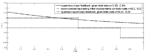
Figure 1: Corresponding analog and quantized supervisory feedback inputs at $z=(0.23,-0.24)$ for constant input $u=1.1$ at symbolic point $x=(0.2,-0.2)$.

Then the corresponding analog supervisory input driving from $z$ is given as $\textbf{u}_{z,x}=1.1+C(\textbf{z}(t)-\textbf{x}(t))$ according to Equation 4. The graph of the analog supervisory input is displayed in Figure 1. By inducing $\textbf{u}_{z,x}$ at $z$, we reach the point $z^{\prime}=(0.56,1.35)$ at time $t=1$. Since $||z^{\prime}-x^{\prime}||=\max\{0.6-0.56,1.4-1.35\}=0.05<\epsilon=0.12$, therefore $z^{\prime}$ is symbolically related to $x^{\prime}$. Thus our assertion that the symbolic model is $0.12$-proximate is validated in this specific example.

Next, we heuristically quantized the supervisory input $\textbf{u}_{z,x}$ to lie in the quantized input trajectory space $\widetilde{\mathcal{U}}$, and obtained the quantized supervisory feedback input displayed in Figure 1. There are also formal approaches to feedback quantization [2, 3, 5]. Driving with the quantized input starting from $z=(0.23,-0.24)$, we reached the point $z^{\prime\prime}=(0.58,1.38)$ at 1 second. Since $||z^{\prime\prime}-x^{\prime}||=\max\{0.6-0.58,1.4-1.38\}=0.02<\epsilon=0.12$, therefore $z^{\prime\prime}$ is also symbolically related to $x^{\prime}$. This means that, for this specific illustration, the proximity of $0.12$ is valid even after quantizing the supervisory input.

From Figure 1, the difference between $\textbf{u}_{z,x}$ and u is less that $0.48=||C||\epsilon=\rho$. Therefore, our assertion in Theorem 4.3.2 is valid for this example. Also the difference between the quantized supervisory feedback input and u is less than $0.48$.

10 Conclusion

While allowing supervisory feedback to relate inputs between two transition systems, we have found a formal way of parametrization of completeness of a state-time quantized symbolic model with respect to the time quantized system model. We demonstrated how sound state-time quantized symbolic models of possibly unstable but stabilizable, bounded input and already input-quantized linear systems can be built with arbitrarily small proximity and trimming (near-completeness), with respect to the time-quantized model. In future, we would like to extend this work to construct sound, near-complete, and proximate symbolic models for non-linear systems.

Appendix

Definition 10.0.1

Let $U\subseteq\mathbb{R}^{m}$ for some $m\in\mathbb{N}$. Then for $n\in\mathbb{N}$, a function $k:\mathbb{R}^{n}\times\mathbb{R}^{n}\times U$ is called a supervisory function iff all the following hold.

1. $k$ is continuously differentiable on $\mathbb{R}^{2n}\backslash\Delta$ where $\Delta=\{(x,x):x\in\mathbb{R}^{n}\}$;

2. $k(y,x,u)=u$ $\forall$ $(y,x)\in\Delta$;

We say that a supervisory function is linear if it is of the form $k(y,x,u)=u+C(y-x)$ for some matrix $C$. It is easy to see that $\left(u+C(y-x)\right)$ moves out of any bounded input set because the supervisory function translates the original input set by an amount $C(y-x)$. Therefore, there can not be a linear supervisory function on a bounded input set.

We now state the general global asymptotic stabilizability assumption and prove that everywhere divergent linear systems with bounded input set can not be globally asymptotically stabilized by any kind of supervisory function.

Notation: A function $\beta:\mathbb{R}_{\geq 0}\times\mathbb{R}_{\geq 0}\rightarrow\mathbb{R}_{\geq 0}$ is called a $\mathcal{KL}_{\infty}$ function if $\beta(r,.)$ is increasing function in $r$ such that $\beta(0,.)=0$; and $\beta(.,t)$ asymptotically tends to zero as $t\rightarrow\infty$.

The following stabilizability assumption, which we call the global asymptotic stabilizability assumption, was discussed in [11].

Definition 10.0.2

A control system with input set $U$ and state space $\mathbb{R}^{n}$ is said to be globally asymptotically stabilizable if there exists a supervisory function $k:\mathbb{R}^{n}\times\mathbb{R}^{n}\times U\rightarrow U$ enforcing the following estimate for all $x,y\in\mathbb{R}^{n}$, $\textbf{u}\in\mathcal{U}$ and $t\in\mathbb{R}_{0}^{+}$

$$||\textbf{x}(t,x,\textbf{u})-\textbf{y}(t,y,k(\textbf{y},\textbf{x},\textbf{u}))||\leq\beta(||x-y||,t).$$ (7)

where $\beta$ is a $\mathcal{KL}_{\infty}$ function.

A linear system $\Sigma=\left<A_{n\times n},B_{n\times m},U,\mathcal{U}\right>$ is everywhere divergent if all the eigenvalues of $A$ have positive real part. Consider $\lambda_{min}$ as the eigenvalue of $A$ with minimum real part. Consider $\Sigma$ as everywhere divergent and so $Re(\lambda_{min})$ is positive. We proceed to demonstrate that for the everywhere divergent linear system $\Sigma$, if the input set $U$ is bounded such that $||u||<M~{}\forall u\in U$, then any two state trajectories starting at a distance greater than $\frac{4||B||M}{Re(\lambda_{min})}$ can never come arbitrarily close, irrespective of what pair of input trajectories drives the two state trajectories. This would mean that the system can not be globally asymptotically stabilized. The proof is as follows.

We know for a linear system

$$\begin{split}\textbf{x}(x,\tau,\textbf{u})-\textbf{y}(y,\tau,\textbf{v})=\exp(A\tau)(x-y)+\int_{0}^{\tau}\exp(A(\tau-t))B(\textbf{u}-\textbf{v})(t)dt\end{split}$$ (8)

By using reverse triangular inequality on (8) we get

$$\begin{split}&\left|\left|\textbf{x}(x,\tau,\textbf{u})-\textbf{y}(y,\tau,\textbf{v})\right|\right|\\ &\geq\left|\left|\exp(A\tau)(x-y)\right|\right|-\left|\left|\int_{0}^{\tau}\exp(A(\tau-t)B(\textbf{u}-\textbf{v})(t)\right|\right|\end{split}$$ (9)

For all possible pairs of trajectories u and v, we have that $\left|\left|\textbf{u}-\textbf{v}\right|\right|\leq 2M$ since the norm of inputs is bounded by $M$.

Then choose $x,y$ such that $||x-y||>\frac{4M||B||}{Re(\lambda_{min})}$. Putting these bounds in (9) we get

$$\begin{split}&\left|\left|\textbf{x}(x,\tau,\textbf{u})-\textbf{y}(y,\tau,\textbf{v})\right|\right|\\ &\geq 2M||B||\left|\left|\exp(A\tau)\left(\frac{2}{Re(\lambda_{min})}-\int_{0}^{\tau}\exp(-At)dt\right)\right|\right|\end{split}$$ (10)

Again using reverse triangular inequality we get

$$\begin{split}&\left|\left|\textbf{x}(x,\tau,\textbf{u})-\textbf{y}(y,\tau,\textbf{v})\right|\right|\\ &\geq 2M||B||||\exp(A\tau)||\left(\frac{2}{Re(\lambda_{min})}-\left|\left|\int_{0}^{\tau}\exp(-At)dt\right|\right|\right)\end{split}$$ (11)

Since $\left|\left|\int_{0}^{\tau}\exp(-At)dt\right|\right|\leq\int_{0}^{\tau}||\exp(-At)||dt$ So

$$\left(\frac{2}{Re(\lambda_{min})}-\left|\left|\int_{0}^{\tau}\exp(-At)dt\right|\right|\right)\geq\left(\frac{2}{Re(\lambda_{min})}-\int_{0}^{\tau}||\exp(-At)||dt\right).$$

Furthermore, we have that $||\exp(-At)||\leq\exp(-Re(\lambda_{min})t)$ since $\lambda_{min}$ is the eigenvalue with minimum real part. Substituting we get

$$\left(\frac{2}{Re(\lambda_{min})}-\left|\left|\int_{0}^{\tau}\exp(-At)dt\right|\right|\right)\geq\left(\frac{2}{Re(\lambda_{min})}-\int_{0}^{\tau}\exp(-Re(\lambda_{min})t)dt\right)$$

$$\geq\left(\frac{2}{Re(\lambda_{min})}-\frac{1}{Re(\lambda_{min})}\right)~{}~{}~{}\text{since}~{}\int_{0}^{\infty}\exp(-Re(\lambda_{min})t)dt=1/Re(\lambda_{min}).$$

Substituting in (11) we get

$$\begin{split}&\left|\left|\textbf{x}(x,t,\textbf{u})-\textbf{y}(y,t,\textbf{v})\right|\right|\geq\frac{2M||B||||\exp(A\tau)||}{Re(\lambda_{min})}\\ \end{split}$$ (12)

$\frac{2M||B||||\exp(A\tau)||}{Re(\lambda_{min})}$ keeps increasing in $\tau$ because $A$ has all eigenvalues with positive real part.

This means that, the linear system being everywhere divergent with norm of inputs upper bounded by $M>0$, if the starting points $x$ and $y$ are such that $||x-y||>\frac{4M||B||}{Re(\lambda_{min})}$ where ${Re(\lambda_{min})}$ is the eigenvalue with minimum real part (which is positive), then x and y can not come arbitrarily close for any possible input trajectories u and v inside the bounded input set driving x and y respectively. This completes the proof.

Hence an everywhere divergent linear system whose input set is bounded can not be globally asymptotically stabilized. But such a system may still be locally asymptotically stabilizable and an example was shown in Section 4. However if the input space has no boundaries, then global asymptotic stabilizability of linear systems is equivalent to local asymptotic stabilizability.

References

- [1] JE Bertram. The effect of quantization in sampled-feedback systems. American Institute of Electrical Engineers, Part II: Applications and Industry, Transactions of the, 77(4):177–182, 1958.
- [2] Roger W Brockett and Daniel Liberzon. Quantized feedback stabilization of linear systems. Automatic Control, IEEE Transactions on, 45(7):1279–1289, 2000.
- [3] David F Delchamps. Stabilizing a linear system with quantized state feedback. Automatic Control, IEEE Transactions on, 35(8):916–924, 1990.
- [4] Gene F Franklin, Michael L Workman, and Dave Powell. Digital control of dynamic systems. Addison-Wesley Longman Publishing Co., Inc., 1997.
- [5] Minyue Fu and Lihua Xie. The sector bound approach to quantized feedback control. Automatic Control, IEEE Transactions on, 50(11):1698–1711, 2005.
- [6] Antoine Girard and George J. Pappas. Approximation metrics for discrete and continuous systems. IEEE Transactions on Automatic Control, 52(5):782 – 798, 2007.
- [7] Manuel Mazo Jr., Anna Davitian, and Paulo Tabuada. PESSOA: A tool for embedded control software synthesis. In Proceedings of the 22nd international conference on Computer Aided Verification, pages 566–569, 2010.
- [8] Rupak Majumdar and Majid Zamani. Approximately bisimilar symbolic models for digital control systems. In Computer Aided Verification, pages 362–377. Springer, 2012.
- [9] Giordano Pola, Antoine Girard, and Paulo Tabuada. Approximately bisimilar symbolic models for nonlinear control systems. Automatica, 44(10):2508–2516, 2008.
- [10] J Slaughter. Quantization errors in digital control systems. Automatic Control, IEEE Transactions on, 9(1):70–74, 1964.
- [11] Paulo Tabuada. An approximate simulation approach to symbolic control. Automatic Control, IEEE Transactions on, 53(6):1406–1418, 2008.
- [12] Yuichi Tazaki and Jun-ichi Imura. Discrete abstractions of nonlinear systems based on error propagation analysis. Automatic Control, IEEE Transactions on, 57(3):550–564, 2012.
- [13] Majid Zamani, Giordano Pola, Manuel Mazo Jr., and Paulo Tabuada. Symbolic models for nonlinear control systems without stability assumptions. IEEE Transactions on Automatic Control, 57(7):1804 – 1809, 2012.