Full quantum mechanical analysis
of atomic three-grating Mach-Zehnder interferometry

Abstract

Atomic three-grating Mach-Zehnder interferometry constitutes an important tool to probe fundamental aspects of the quantum theory. There is, however, a remarkable gap in the literature between the oversimplified models and robust numerical simulations considered to describe the corresponding experiments. Consequently, the former usually lead to paradoxical scenarios, such as the wave-particle dual behavior of atoms, while the latter make difficult the data analysis in simple terms. Here these issues are tackled by means of a simple grating working model consisting of evenly-spaced Gaussian slits. As is shown, this model suffices to explore and explain such experiments both analytically and numerically, giving a good account of the full atomic journey inside the interferometer, and hence contributing to make less mystic the physics involved. More specifically, it provides a clear and unambiguous picture of the wavefront splitting that takes place inside the interferometer, illustrating how the momentum along each emerging diffraction order is well defined even though the wave function itself still displays a rather complex shape. To this end, the local transverse momentum is also introduced in this context as a reliable analytical tool. The splitting, apart from being a key issue to understand atomic Mach-Zehnder interferometry, also demonstrates at a fundamental level how wave and particle aspects are always present in the experiment, without incurring in any contradiction or interpretive paradox. On the other hand, at a practical level, the generality and versatility of the model and methodology presented, makes them suitable to attack analogous problems in a simple manner after a convenient tuning.

1 Introduction

Matter-wave interferometry constitutes an important application of quantum interference with both fundamental and practical interests [1, 2, 3, 4, 5, 6]. In analogy to optics, this sensitive technique allows us to determine properties of the diffracted particles as well as of any other element acting on them during their transit through the interferometer. It was at the beginning of the 1990s when Kasevich and Chu [7] showed that matter-wave Mach-Zehnder interferometry can be achieved by using the same basic ideas of its optical analog: if the atomic wave function can be coherently split up, and later on each diffracted wave is conveniently redirected in order to eventually achieve their recombination on some space region, then an interference pattern will arise on that spot. For neutral atoms this can be done by means of periodic gratings, which play the role of optical beam splitters. This property, exploited in different diffraction experiments with fundamental purposes [8, 9, 10, 11, 12], gave rise to the former experimental implementations of atomic Mach-Zehnder interferometers in the early 1990s, first with transmission gratings [13] and then with light standing waves [14]. These interferometers are based on a very efficient production of spatially separated coherent waves [15]. Similar interferometers are also used for large molecules [16, 17, 18], although due to their relatively smaller thermal wavelength, they work within the near field or Fresnel regime, benefiting from the grating self-imaging produced by the so-called Talbot-Lau effect [19, 20], a combination of the Talbot [21, 22, 23, 24] and Lau [25, 26, 27] effects.

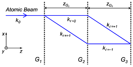
Figure 1: Sketch of an atomic three-grating Mach-Zehnder interferometer. This class of interferometers consists of three equally-spaced ($z_{G_{2}}=z_{G_{3}}$), parallel gratings, namely $G_{1}$, $G_{2}$, and $G_{3}$. These gratings play the role of the set of beam splitters ($G_{1}$ and $G_{3}$) and mirrors ($G_{2}$) of a conventional optical interferometer.

To describe and analyze this kind of experiments different analytical and numerical treatments have been proposed in the literature [2, 3, 4, 28]. Nonetheless, there is a substantial gap between simple models and exact numerical simulations, which makes difficult getting a unified view of the physics involved in these experiments. Consequently, many times our understanding of them is oversimplified, which leads us to emphasize “paradoxical” aspects of quantum mechanics. One of these aspects is, for example, the commonly assumed wave-particle dual nature of quantum systems. Depending on how the experiment is performed, one “decides” between one or the other, which manifests as one or another type of outcome. Now, leaving aside ontological issues, a pragmatic, accurate description of the experiment requires the use of a wave function. The evolution of this wave function in the course of the experiment is strongly influenced by the boundary conditions associated with such an experiment, as well as by any other physical effect that might take place (e.g., presence of photon scattering events [4]), which will unavoidably lead to different outcomes. That is, any trace of paradox disappears if we just focus on the wave function and all the factors that affect it during the performance of the experiment — we obtain what should be obtained, leaving not much room for speculating about dual behaviors. This is precisely the scenario posed by atomic Mach-Zehnder interferometers, where it is common to describe the evolution between consecutive gratings in terms of classical-like paths (see Fig. 1), although their recombination (and, actually, also their emergence) has to do with a pure wave-like behavior.

Moved by these facts and their important implications, here we revisit the problem with a working model consisting of a set of three gratings with Gaussian slits (slits characterized by a Gaussian transmission function), while its analysis is conducted by means of a combination of the position and momentum representations of the (atomic) wave function. As is shown, the synergy between analytical results and numerical simulations obtained in this way helps to describe and understand the functioning of these interferometers in a relatively simple manner. Specifically, we provide a clear picture of the wavefront splitting process that takes place at the gratings, showing how the typical path-like picture of the interferometer [29] (see Fig. 1) coexists with the complex interference patterns exhibited by the wave function between consecutive gratings. This is a key point to understand the simplified models commonly used in the literature to explain this type of interferometers, where the particular shape of the wave function is neglected and only the momentum carried along the paths associated with each involved diffraction order is considered. In this regard, we have introduced the concept of local transverse momentum, borrowed from the Bohmian formulation of quantum mechanics [30], as analytical tool. By means of this quantity it is possible to properly quantify the local value of the momentum (not to be confused with the usual momentum expectation value) at each point of the transverse coordinate, which is related to the quantum flux [31, 32] evaluated on that point. Furthermore, we would also like to stress the practical side of this model as an efficient tool to attack analogous problems with presence of incoherence sources and/or decoherent events in a simple manner.

This work has been organized as follows. The general theoretical elements involved in our analysis of the atomic three-grating Mach-Zehnder interferometer are described in Sec. 2, including the Gaussian grating model considered. Analytical results obtained from this model in the far field are presented and discussed in Sec. 3. The outcomes from the numerical simulations illustrating different aspects of the wave-function full evolution between consecutive gratings are analyzed and discussed in Sec. 4. The conclusions from this work are summarized in Sec. 5.

2 Theory

2.1 General aspects of grating diffraction

Atomic three-grating Mach-Zehnder interferometers consist of three evenly-spaced and parallel periodic gratings, as it is illustrated in Fig. 1. In this sketch the slits are parallel to the $y$ axis and span a relatively long distance (larger than the cross-section of the incident beam). This implies translational invariance along the $y$ axis, which makes diffraction to be independent of this coordinate and allows a reduction of the problem dimensionality to the transverse ($x$) and longitudinal ($z$) directions. Under realistic experimental working conditions, taken from the former 1991 experiment by Keith et al. [13] (see Sec. 2.2), the propagation of the atomic beam along the longitudinal direction is typically faster than its translational spreading [33]. From the experimental data reported in [13], we notice that the distance between consecutive gratings is of the order of half a meter, while the separation between consecutive diffraction orders is about a few tenths of microns. These are just paraxial conditions, which allow us to decouple the transverse and longitudinal (translational) degrees of freedom for practical purposes. This assumption not only simplifies the analytical treatment, but also provides us with a neater dynamical picture of the emergence of well-resolved diffraction orders and their subsequent recombination (see Sec. 4), avoiding the complexities involved by reflections at the gratings [34]. Also for simplicity, short-range interactions between the diffracted particles and the grating [34, 35], as well as imperfections or thermal effects associated with the latter [17, 36, 37], are neglected in this work, although they can be easily implemented by varying some of the parameters of the model (see discussion in this regard in Sec. 2.2).

The atoms leaving the source follow a Boltzmann velocity distribution at a temperature $T$, which implies an associated average thermal de Broglie wavelength $\lambda=2\pi\hbar/\sqrt{3mk_{B}T}$. Although the beam is not fully monochromatic under these conditions, the presence of two consecutive collimating slits beyond the source leads to a nearly plane (monochromatic) wavefront behind the second of these slits. This is the beam impinging on $G_{1}$. In spite of possible deviations from full monochromaticity, for practical purposes and analytical simplicity we assume that this beam is nearly monochromatic. Accordingly, if $k^{2}=k_{x}^{2}+k_{z}^{2}$, where $k=2\pi/\lambda$, we can assume that $k_{z}\gg k_{x}$ and $k\approx k_{z}$. This allows us to express the atomic wave function at any time as a product state,

$$\Psi(x,z,t)\approx\psi(x,t)e^{ik_{z}z-iE_{z}t/\hbar}.$$ (1)

The longitudinal component is a plane wave with average momentum $p_{z}=\hbar k_{z}$ and energy $E_{z}=p_{z}^{2}/2m=\hbar k_{z}^{2}/2m$. The transverse component, $\psi(x,t)$, is a solution of the time-dependent, free-particle Schrödinger equation

$$i\hbar\ \frac{\partial\psi}{\partial t}=-\frac{\hbar^{2}}{2m}\frac{\partial^{2}\psi}{\partial x^{2}},$$ (2)

with initial condition $\psi(x,0)$.

Solutions of Eq. (2) can be readily found by computing the Fourier transform of $\psi(x,t)$ [30],

$$\psi(x,t)=\frac{1}{\sqrt{2\pi}}\!\int\tilde{\psi}(k_{x},t)e^{ik_{x}x}dk_{x}.$$ (3)

Physically this is just a way to recast $\psi(x,t)$ as a linear combination or superposition of plane waves, $e^{ik_{x}x}$, each one contributing with a weight and phase specified by $\tilde{\psi}(k_{x},t)$. Notice that $\tilde{\psi}(k_{x},t)$ is just the representation of the wave function in the momentum (reciprocal) space, which depends on the reciprocal variable or momentum $k_{x}$. Substituting (3) into Eq. (2) leads to

$$i\hbar\ \!\frac{\partial\tilde{\psi}}{\partial t}=\left(\frac{\hbar^{2}k_{x}^{2}}{2m}\right)\tilde{\psi},$$ (4)

which, after integration in time, yields

$$\tilde{\psi}(k_{x},t)=\tilde{\psi}(k_{x},0)e^{-i\hbar k_{x}^{2}t/2m}.$$ (5)

The initial condition $\tilde{\psi}(k_{x},0)$ corresponds to the representation of the initial wave function, $\psi(x,0)$, in the momentum space,

$$\tilde{\psi}(k_{x},0)=\frac{1}{\sqrt{2\pi}}\!\int\psi(x,0)e^{-ik_{x}x}dx.$$ (6)

The solution (5), with initial condition (6), allows us to rearrange Eq. (3) as

$$\psi(x,t)=\sqrt{\frac{m}{2\pi i\hbar t}}\int\psi(x^{\prime},0)e^{im(x-x^{\prime})^{2}/2\hbar t}dx^{\prime}.$$ (7)

after integrating in $k_{x}$. Notice in this latter expression that the quantity

$$\mathcal{K}(x,x^{\prime})\equiv\sqrt{\frac{m}{2\pi i\hbar t}}\ \!e^{im(x-x^{\prime})^{2}/2\hbar t}$$ (8)

corresponds to the free-particle kernel or propagator, which can be alternatively obtained by means of a rather longer way using path integrals [38].

Given that the longitudinal component of the wave function is a plane wave that propagates with velocity $v=\hbar k_{z}/m\approx\hbar k/m$, the problem can be reparameterized in terms of the longitudinal coordinate, $z$. That is, the wave function (7) describing the wave function evolution along the transverse direction (accounted for by the $x$ coordinate) can be recast in terms of this coordinate,

$$\psi(x,z)\approx\sqrt{\frac{k}{2\pi iz}}\int\psi(x^{\prime},0)e^{ik(x-x^{\prime})^{2}/2z}dx^{\prime},$$ (9)

with $z=vt\approx(\hbar k/m)t$. This form is mass-independent and therefore can be used advantageously to describe massive particles as well as light (when the latter is described by a scalar field [39]).

The difference between various problems is established by the initial condition $\psi(x,z_{0})$, where $z_{0}$ denotes the starting position along the $z$ axis from which the (transverse) wave function starts its propagation. If the gratings are assumed to be infinitesimally thin along the longitudinal direction, we can consider a simple relationship between the ansatz and the incident wave function:

$$\psi_{G}(x,z_{0})=\hat{T}_{G}\{\psi_{\rm inc}^{G}(x,z_{0})\},$$ (10)

where $\psi_{G}(x,z_{0})$ is the ansatz (diffracted) wave function just behind the grating $G$ (located at $z_{0}$), $\hat{T}_{G}$ is the transmission operator characterizing $G$, and $\psi_{\rm inc}^{G}(x,z_{0})$ is the wave function incident onto $G$. The transmission operator plays here a role analogous to that of the scattering operator or S-matrix in scattering theory [40]; the details of its action on the incident wave function are described below in the context of Gaussian-slit gratings. Now, taking into account Eq. (10), the propagation between two consecutive gratings, given by Eq. (9), acquires the functional form:

$$\psi_{G}(x,z)=\sqrt{\frac{k}{2\pi iz}}\!\int\hat{T}_{G}\{\psi_{\rm inc}^{G}(x^{\prime},z_{0})\}e^{ik(x-x^{\prime})^{2}/2z}dx^{\prime}.$$ (11)

For practical purposes, and without loss of generality, later on the problem will be piecewise solved, particularizing Eq. (11) to the transit from $G_{1}$ to $G_{2}$ ($\psi_{G_{1}}$) and from $G_{2}$ to $G_{3}$ ($\psi_{G_{2}}$). For both transits the origin will be set at the corresponding grating (i.e., $z_{0}=0$ in both cases). As for the incident wave functions, $\psi_{\rm inc}^{G_{1}}(x,0)$ will be an incoming plane wave, while $\psi_{\rm inc}^{G_{2}}(x,0)=\psi_{G_{1}}(x,z_{G_{2}})$.

In general the integral (11) cannot be solved analytically except for Gaussian states. Nonetheless, in the far field ($f\!f$) or Fraunhofer regime it acquires a simpler form and admits some additional analytical solutions [41]. In this regime, we have $x\gg x^{\prime}$ and therefore the phase factor of Eq. (9) can be approximated by

$$\frac{k(x-x^{\prime})^{2}}{2z}\approx\frac{kx^{2}}{2z}-\frac{kxx^{\prime}}{z}.$$ (12)

This allows to recast Eq. (9) as

$$\psi_{G}^{f\!f}(x,z)\approx\sqrt{\frac{k}{2\pi iz}}\ \!e^{ikx^{2}/2z}\!\int\psi(x^{\prime},0)e^{-ik_{x}x^{\prime}}dx^{\prime},$$ (13)

where we introduce the definition $k_{x}=kx/z$, with $x/z$ being the direction cosine [42] with respect to the origin at the grating $G$ (another physical explanation will be provided for this choice of identifying $k_{x}$ with a transverse momentum; see Sec. 4.1). Comparing this integral with (6), we find that except for a phase factor the wave function in the far field is proportional to the representation of the initial wave function in the momentum space:

$$\psi_{G}^{f\!f}(x,z)\approx\sqrt{\frac{k}{iz}}\ \tilde{\psi}_{G}(k_{x})e^{ikx^{2}/2z}.$$ (14)

Fraunhofer diffraction can then be understood as the Fourier image of the initial wave function. Physically, this means that in the far field (asymptotically) the global shape of the probability density is independent of the distance from the grating, mimicking the transverse momentum distribution: $|\psi_{G}^{f\!f}(x,z)|^{2}\propto|\tilde{\psi}_{G}(k_{x})|^{2}$. In other words, the aspect ratio of the wave function remains invariant with $z$ or, equivalently, with time. Furthermore, because $\tilde{\psi}_{G}(k_{x})$ is related to the grating transmission, the far-field wave function is just a manifestation of the grating structure, thus providing us with information about it and not only about properties of the diffracted atom. Note the analogy with optics [43], where the wave amplitude in the far field or Fraunhofer regime is just the Fourier transform of the aperture function evaluated at a spatial frequency precisely given by $k_{x}$.

Regarding the phase factor that appears in Eq. (14), it has not been recast in terms of $k_{x}$ on purpose, because of its quadratic dependence on $x$. As it can be noticed, if we apply the usual (transverse) momentum operator, $\hat{p}_{x}=-i\hbar\partial/\partial x$ to (14), we find

$$\hat{p}_{x}\psi_{G}^{f\!f} \propto \left(\frac{\hbar kx}{z}\ \tilde{\psi}_{G}-\frac{i\hbar k}{z}\frac{\partial\tilde{\psi}_{G}}{\partial k_{x}}\right)e^{ikx^{2}/2z}$$ (15)

$$= \frac{\hbar k}{z}\left[\int(x-x^{\prime})\psi(x^{\prime},0)e^{-ik_{x}x^{\prime}}dx^{\prime}\right]e^{ikx^{2}/2z}$$

$$\propto \frac{\hbar kx}{z}\ \psi_{G}^{f\!f}=\hbar k_{x}\psi_{G}^{f\!f},$$

where we have considered the equality $\partial/\partial x=(\partial k_{x}/\partial x)\partial/\partial k_{x}=(k/z)\partial/\partial k_{x}$ in the first line, and the approximation $x\gg x^{\prime}$ in the last step. Hence, to some extent it can be said that the far-field wave function evolves locally (at each point) as an effective plane wave with (effective) momentum $p_{x}=\hbar kx/z=\hbar k_{x}$ (see Sec. 4.1). Taking this into account, Eq. (14) can be recast in terms of plane waves, as

$$\psi_{G}^{f\!f}(x,z)\propto\tilde{\psi}_{G}(k_{x})e^{ik_{x}x}.$$ (16)

2.2 The Gaussian grating model

In order to get a more quantitative idea on the amplitude splitting process and the subsequent recombination, now we are going to introduce a simple model consisting of three identical periodic gratings with Gaussian slits. By Gaussian slit we just mean a slit characterized by a Gaussian transmission function [38, 44], i.e., a transmission which is maximum at the center of the slit and decreases smoothly in a Gaussian fashion towards the slit boundaries. This behavior can be observed, for example, in situations where the problem is tackled from a scattering viewpoint and the interaction between the slit and the diffracted particle is modeled by means of a realistic interaction soft potential [34, 35]. Gaussian transmissions are also in compliance with the fact that the incident beam is not fully monochromatic (see Sec. 2), which leads to a relatively fast decay (actually, in a Gaussian fashion) of eventual diffraction orders as we move apart from the incident propagation direction (in agreement with real matter wave experimental observations). As it will be seen, this model is very convenient both analytically and numerically. Regarding the value of the different physical parameters, we have considered without loss of generality those reported by Keith et al. [13] in their former experiment on three-grating Mach-Zehnder interferometry with sodium atoms. Accordingly, the thermal de Broglie wavelength of the sodium atoms is $\lambda=16$ pm ($k=0.393$ pm^-1), the grating period is $d=0.4$ $\mu$m, the slit width is $w=0.2$ $\mu$m, and the distance between two consecutive gratings is $L=0.663$ m.

The action of the transmission operator on an incident wave function is modeled as

$$\hat{T}_{G}\{\psi_{\rm inc}\}=\sum_{j=1}^{N}\beta_{j}\ \!e^{-(x-x_{j})^{2}/4\sigma_{0}^{2}+ik_{j,x0}x},$$ (17)

i.e., each slit produces a Gaussian diffracted wave with a width $\sigma_{0}=w/2$, such that it covers an effective distance of $d/2$ (it is almost zero at $x=x_{j}\pm w/2$). If $\psi_{\rm inc}^{G}$ is not a plane wave, the amount of probability transmitted through each slit will be different. In order to account for this fact, we introduce an opacity parameter $\beta_{j}$ specifying how much the $j$th slit (i.e., the slit centered at $x_{j}$) contributes to the total diffracted wave function. In particular, here we have considered $\beta_{j}=|\psi_{\rm inc}^{G}(x_{j},z_{0})|/\sqrt{{\rm max}\{|\psi_{\rm inc}^{G}(x,z_{0})|^{2}\}}$. In this contexts, $N$ must be understood as the total, effective number of slits that contribute to the diffracted wave (we have neglected contributions from slits such that their associated $\beta$ are below a certain onset). Finally, it can also happen that the transverse momentum varies locally along $\psi_{\rm inc}^{G}$. This effect is taken into account by associating a momentum $k_{j,x0}$ with each Gaussian wave, with its value being determined by the local momentum of $\psi_{\rm inc}^{G}$ at the center of the $j$th slit. As shown below, this model is very convenient both analytically and computationally.

In order to show how the model works in a simple case, consider that the wave function incident onto $G_{1}$ is a plane wave given by

$$\psi_{\rm inc}^{G_{1}}(x,0)\sim e^{ik_{x0}x},$$ (18)

where $k_{x0}=k_{0}\sin\theta$, with $\theta$ being the angle between the $z$ axis and the direction of the incident wave vector (later on we will particularize to the case of normal incidence, so that $k_{x0}=0$). For example, according to the experiment, the passage of the sodium atoms through two 20-$\mu$m–slits produces a collimated beam of about 20 $\mu$ width, which covers about 50 slits at $G_{1}$. In this sense Eq. (18) constitutes a reliable guess. After its substitution into (17), with $\beta_{j}=1$ and $k_{j,x0}=k_{x0}$ for all $j$, we obtain the ansatz (10) behind $G_{1}$ (i.e., the initial, diffracted wave function), which is a coherent superposition of Gaussian wave packets,

$$\psi_{G_{1}}(x,0)\approx\frac{1}{\sqrt{N}}\sum_{j=1}^{N}\left(\frac{1}{2\pi\sigma_{0}^{2}}\right)^{1/4}e^{-(x-x_{j})^{2}/4\sigma_{0}^{2}+ik_{x0}x}.$$ (19)

In this expression, the symbol “$\approx$” comes from the fact that all the overlapping terms in the normalization condition are assumed to be negligible. The prefactors $1/\sqrt{N}$ and $(2\pi\sigma_{0}^{2})^{-1/4}$ are introduced in order to keep $\psi_{G_{1}}$ normalized. The opacities have all been set equal to one, because the probability density associated with the plane wave (18) is uniform. As it is described in more detail in Sec. 4.2, in the passage through $G_{2}$ the value of the opacity factors is not homogenous, since the probability density associated with the wave function reaching this grating is not uniform along $x$. More importantly, the particular functional form displayed by Eq. (19) makes evident where nonlocality enters the problem, by specifying the nonseparable connection between the local value of the wave function at any point $x$ with the simultaneous action of the partial waves coming from each slit (centered at spatially separated points $x_{j}$). This combined action has not only to do with a probability density, but with the generation of an overall phase field that governs the dynamical evolution of the wave function at each point of the configuration space and can be measured through the local value of the transverse momentum (see Sec. 4.1).

3 Far-field analytical results

3.1 Beam splitting and subsequent recombination

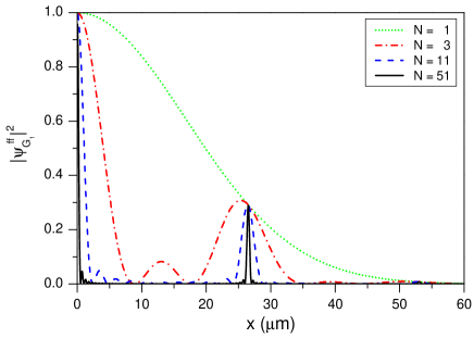
Figure 2: Probability density $|\psi_{G_{1}}^{f\!f}(x,z)|^{2}$, given by Eq. (20), evaluated at $z=z_{G_{2}}=0.663$ m for different values of the number of slits (see legend); notice that the green dotted line corresponds to the Gaussian single-slit envelope. For an easier comparison, the maximum intensity has been set to one in all cases.

The paths depicted in Fig. 1 behind $G_{1}$ or $G_{2}$ constitute a convenient and simplified representation of the tracks followed by the different diffraction orders that develop from the transmitted atomic wave function. To understand the origin of these paths we need to focus on how this wave function evolves in the far field, where its shape only depends on the aspect ratio $x/z$, as it is indicated by Eq. (16). With this in mind, let us first consider the transit between $G_{1}$ and $G_{2}$. Provided the far-field condition (12) is fulfilled, we can start describing the behavior of the wave function between these two gratings directly from Eq. (16). If $x_{j}=x_{0}+(j-1)d$, with $x_{0}=-(N-1)d/2$ for convenience (the origin $x_{0}$ is irrelevant, since it only adds a global phase factor), we find

$$\psi_{G_{1}}^{f\!f}(x,z)\propto\left[\frac{\sin(\Delta k_{x}Nd/2)}{\sin(\Delta k_{x}d/2)}\right]e^{-\sigma_{0}^{2}\Delta k_{x}^{2}},$$ (20)

where $\Delta k_{x}=k_{x}-k_{x0}$. In this expression, the term between square brackets describes the interference produced by the coherent superposition of the $N$ diffracted waves, while the exponential (envelope) term accounts for the diffraction associated with a single Gaussian slit. Equation (20) displays a series of principal maxima whenever $k_{x}=k_{x,\ell}=k_{x0}+2\pi\ell/d$ (vanishing denominator), with $\ell=0,\pm 1,\pm 2,\ldots$, which give rise to the corresponding diffraction orders (other secondary maxima also appear in between, but become meaningless as $N$ increases and are therefore physically irrelevant). The intensity of these diffraction orders depends on how fast the Gaussian envelope (see the green dotted line in Fig. 2) falls. The ratio of intensities for these maxima with respect to the zeroth diffraction order can be readily determined [45], reading

$$\mathcal{R}_{0,\ell}=\frac{|\psi_{G_{1},\ell}^{f\!f}(x,z)|^{2}}{|\psi_{G_{1},0}^{f\!f}(x,z)|^{2}}=e^{-2(2\pi\ell\sigma_{0}/d)^{2}}.$$ (21)

When numerical values are substituted into this expression, we find that the intensity for $\ell=\pm 1$ is about 70% weaker than for the zeroth-order one ($\mathcal{R}_{0,\pm 1}\approx 0.29$), and that for $\ell=\pm 2$ it is essentially negligible ($\mathcal{R}_{0,\pm 2}\approx 7.2\times 10^{-3}$). In other words, the grating produces an effective splitting of the amplitude of the incoming wave function into three well separated wavefronts. The diffraction orders $\ell=0$, $\ell=+1$, and $\ell=+2$ are displayed in Fig. 2 for different values of $N$.

Given the linear relationship between $x$ and $z$ in the far field, the position of the diffraction orders at a distance $z$ from the grating is determined by

$$x_{\ell}=\left(\frac{k_{x,\ell}}{k}\right)z=\left(\frac{k_{x0}}{k}+\frac{\ell\lambda}{d}\right)z.$$ (22)

The width of the corresponding intensity peaks, measured between the two adjacent minima, is given by

$$\Delta x=\left(\frac{2\lambda}{Nd}\right)z,$$ (23)

which depends on $N$ (it decreases as $N$ increases), but not on the incident wave vector, $k_{x0}$. Substituting the numerical parameters given in Sec. 2.2 into these expressions, we find that Eq. (22) reads as $x_{\ell}=40\times 10^{-6}\ell z$. That is, at a distance $z=z_{G_{2}}=0.663$ m from $G_{1}$, the two relevant diffraction orders reach the positions $x_{\pm 1}\approx\pm 25.42$ $\mu$m $\approx\pm 66d$, with a width $\Delta x\approx 53.04N^{-1}$ $\mu$m $\approx 133(d/N)$. This means that, in principle, if the far-field condition is fulfilled, the width of the diffraction orders becomes negligible with $N$ (see Fig. 2) and their evolution along $z$ can be approximated by the paths displayed in Fig. 1. In this figure, the two paths between $G_{1}$ and $G_{2}$ represent the evolution along $z$ of the diffraction orders $\ell=0$ and $\ell=+1$. Of course, only far from $G_{1}$ this representation in terms of separated paths is be correct (see Sec. 4). Nonetheless, notice that because of the Gaussian envelope in Eq. (20) it is expected a slight shift of the position described by Eq. (22). As seen in Fig. 2, particularly for $\ell=+1$ (for $\ell=+2$ the intensity is negligible), this effect decreases as $N$ increases, since the peak becomes narrower and narrower, eventually approaching a $\delta$-function.

The amplitude splitting between $G_{1}$ and $G_{2}$ also takes place between $G_{2}$ and $G_{3}$, thus closing the two “arms” of the interferometer. More specifically, what happens is that the two diffraction orders that reach $G_{2}$ around $x_{0}$ and $x_{+1}$ give rise to two diffracted waves around them. Our description after $G_{2}$ can then be formulated in terms of a coherent superposition of two spatially separated waves, each one leading again to a series of diffraction orders. Let $\ell^{(0)}$ and $\ell^{(+1)}$ be the labels for the diffraction orders coming from the waves diffracted around $x_{0}$ and $x_{+1}$, respectively. We notice that the diffraction orders $\ell^{(0)}=+1$ and $\ell^{(+1)}=-1$ eventually coalesce on the same spot or region on $G_{3}$ around $x_{G_{3}}=25.42$ $\mu$m. As seen in Fig. 1, these two paths complete the Mach-Zehnder like structure of the atomic three-grating interferometer.

3.2 Measurement role of the third grating

Once the interferometer structure is demonstrated, one may wonder about the role played by the third grating. This grating can be laterally displaced, which allows us to modify the flux of transmitted atoms around $x_{G_{3}}$, as already shown by Carnal and Mlynek [46]. Notice that unlike the maximum structures that appear around $x=0$ $\mu$m or $x\approx 51$ $\mu$m (the spots respectively reached by the zeroth diffraction order of each wave), the coalescence of $\ell^{(0)}=+1$ and $\ell^{(+1)}=-1$ produces an interference pattern with the same period $d$ of the gratings. This can be easily shown as follows. The momenta of these diffraction orders are

$$k_{x,\ell^{(0)}=+1} = k_{x,0}+2\pi/d=2\pi/d,$$ (24)

$$k_{x,\ell^{(+1)}=-1} = k_{x,+1}-2\pi/d=0,$$ (25)

where $k_{x,0}$ and $k_{x,+1}$ are the zeroth-order momenta associated with each one of the diffracted waves. The corresponding momentum transfers are then equal, but opposite in sign, i.e., $\Delta k_{x,\ell^{(0)}=+1}=k_{x,\ell^{(0)}=+1}-k_{x,0}=2\pi/d$ and $\Delta k_{x,\ell^{(+1)}=-1}=k_{x,\ell^{(+1)}=-1}-k_{x,+1}=-2\pi/d$. If Eq. (20) is evaluated replacing $G_{1}$ by $G_{2}$ (now the starting point is $G_{2}$) and taking into account the above momentum values into account, we find the far-field expression for the two diffraction orders around $x_{G_{3}}$:

$$\psi_{G_{2},\ell^{(0)}=+1}^{f\!f}(x) \propto e^{-(2\pi\sigma_{0}/d)^{2}}e^{2i\pi x/d},$$ (26)

$$\psi_{G_{2},\ell^{(+1)}=-1}^{f\!f}(x) \propto e^{-2(2\pi\sigma_{0}/d)^{2}}.$$ (27)

The extra factor 2 in the argument of the exponential of $\psi_{G_{2},\ell^{(+1)}=-1}^{f\!f}$ arises from the exponential prefactor inherited from the transit between $G_{1}$ and $G_{2}$. The coherent superposition that we find around $x_{G_{3}}$ is

$$\psi_{G_{3}}(x)\sim\psi_{G_{2},\ell^{(0)}=+1}^{f\!f}(x)+\psi_{G_{2},\ell^{(+1)}=-1}^{f\!f}(x)\propto\left[1+e^{-(2\pi\sigma_{0}/d)^{2}}e^{-2i\pi x/d}\right]e^{2i\pi x/d},$$ (28)

which gives rise to an interference pattern, described by

$$|\psi_{G_{3}}(x)|^{2} \propto 1+{\rm sech}[(2\pi\sigma_{0}/d)^{2}]\ \!\cos(2\pi x/d).$$ (29)

(Here we prefer the new denomination $\psi_{G_{3}}$ instead of $\psi_{G_{2}}^{f\!f}$ because the latter refers to the full far-field wave function reaching $G_{3}$ from $G_{2}$, while $\psi_{G_{3}}$ only refers to the section of the wave function $\psi_{G_{2}}^{f\!f}$ around $x_{G_{3}}$.) There is no full fringe visibility because each beam reaches the region around $x_{G_{3}}$ with a different intensity, although the period of the fringes is $d$, as it is for the gratings. This is the reason why the spot around $x_{G_{3}}$ is the interesting one regarding interferometry. Because of this periodicity any perturbation happening inside the interferometer (i.e., among the gratings) eventually translates into a loss of fringe visibility and/or a phase shift [47].

As formerly done by Carnal and Mlynek [46], the number or flux of transmitted atoms can be measured taking advantage of the interference pattern around $x_{G_{3}}$. By keeping $G_{3}$ aligned or misaligned with this interference pattern, the total outgoing atomic flux collected behind this grating will be larger or smaller, respectively. The grating $G_{3}$ then acts like a mask to sample the interference pattern. Thus, consider that the misalignment along the $x$ direction is measured in terms of a variable $\chi$, such that $\chi=0$ means perfect alignment of $G_{3}$ with the interference pattern, and $\chi=d/2$ is maximum misalignment. The amount of atoms passing through $G_{3}$ will depend on $\chi$, and so the total flux collected behind $G_{3}$. The total flux is obtained from a convolution integral:

$$\mathcal{T}_{G_{3}}(\chi)=\int|\psi_{G_{3}}(x)|^{2}T_{G_{3}}(\chi-x)dx\propto 1+2\left[1+e^{-2(2\pi\sigma_{0}/d)^{2}}\right]^{-1}\cos(2\pi\chi/d),$$ (30)

where the subscript $G_{3}$ means that the flux is measured at $z_{G_{3}}$, and $T_{G_{3}}$ is the transmission function associated with this grating, which consists just of a bare sum of Gaussians [i.e., as in Eq. (17), but with $\beta_{j}=0$ and $k_{j,x0}=0$ for all $j$]. Notice that although $\mathcal{T}_{G_{3}}$ displays a similar functional form to the probability density (29), it is a different quantity: it measures the amount of transmitted intensity (number of atoms) as a function of the position of the grating $G_{3}$ with respect to the interference pattern (29). Nonetheless, one can measure the flux for different values of $\chi$ beyond $d$, and the measurements collected will be in direct correspondence with the interference pattern. An analogous functional form to Eq. (30), also displaying the same periodicity, was previously numerically found [39, 48] for slit transmission functions described by hat-functions instead of Gaussians. As a final remark, we would like to note that in the integral (30) no assumption on the spatial extension of the spot around $x_{G_{3}}$ has been introduced. Obviously, the interference pattern (29) has a finite spatial extension that has to be taken into account. In the simulations below the limits of Eq. (30) have been chosen in such a way that no contributions from nearby diffraction orders (around $x=0$ $\mu$m or $x\approx 51$ $\mu$m) “contaminate” the flux related to this interference pattern.

4 Numerical analysis

4.1 Methodology

How close are the previous analytical results to the actual evolution of the atomic wave function inside the interferometer? In order to investigate this question, we decided to perform a series of numerical simulations that illustrate both the full evolution of the wave function between gratings. We would like to stress that the model that we are using is fully analytical (the integration in time of each diffracted Gaussian wave packet $\psi_{j}$ is fully analytical [49]), and therefore the numerical issue only concerns the evaluation of the superpositions or the calculation of some associated quantities. Thus, it can be readily shown that the use of Eq. (7), or equivalently Eq. (11), leads to the analytical solution

$$\psi_{G_{1}}(x,z)\approx\frac{1}{\sqrt{N}}\left(\frac{1}{2\pi\tilde{\sigma}_{z}^{2}}\right)^{1/4}\sum_{j=1}^{N}e^{-(x-x_{j,z})^{2}/4\sigma_{0}\tilde{\sigma}_{z}+ik_{x0}(x-x_{j,z})+ik_{x0}x_{j}+ik_{x0}^{2}z/2k},$$ (31)

where $x_{j,z}=x_{j}+(\hbar k_{x0}/mv)z=x_{j}+(k_{x0}\lambda/2\pi)z$ and $\tilde{\sigma}_{z}=\sigma_{0}[1+(iz/2k\sigma_{0}^{2})]$. In particular, for this initial state we have chosen $\beta_{j}=1$ for all $j$; all the slits are assumed to be identical (see Sec. 2.2). This expression is very useful in the analytical derivation of some diffraction properties in the near and far fields, as it has been done elsewhere in more detail [50].

To inquire questions specifically related to the local transverse momentum (in terms of the wave vector), we are going to introduce the new function $K_{x}$, defined as

$$K_{x}(x,z)={\rm Im}\left[\frac{1}{\psi(x,z)}\frac{\partial\psi(x,z)}{\partial x}\right],$$ (32)

which provides the value of the local transverse momentum $K_{x}$ as a function of the $x$ coordinate at a given distance $z$ from a grating (or whichever the $z$-axis origin is). Notice that this momentum is connected to the usual quantum flux,

$$J_{x}=\frac{\hbar}{m}\ {\rm Im}\left[\frac{1}{\psi}\frac{\partial\psi}{\partial x}\right]=\frac{\hbar}{m}\ K_{x}|\psi|^{2},$$ (33)

commonly used in the Bohmian formulation of quantum mechanics [30]. In the far field, for example, it typically coincides with the transverse momentum value associated with the different diffraction orders, as it can readily be seen by substituting the ansatz (31) into Eq. (32) and then considering the corresponding limits [50]. This renders

$$K_{x}(x,z)\approx k_{x,\ell}.$$ (34)

Analogously, if we substitute the far-field expression (14) into (32), we find

$$K_{x}(x,z)=\frac{kx}{z}=k_{x},$$ (35)

which justifies our choice of $k_{x}$ and the recast of Eq. (14) as (16) in Sec. 2.2.

4.2 Results

In order to show the reliability on the far-field expression given by Eq. (20) at $z=z_{G_{2}}=0.663$ $\mu$m, where the grating $G_{2}$ is placed, the probability density $|\psi_{G_{1}}(x,z_{G_{2}})|^{2}$ is plotted in Fig. 3(a) for $N=3$ (red dashed-dotted line) and $N=11$ (blue dashed line), and in Fig. 3(b) for $N=51$ (we have split up the graph for visual clarity). When comparing the results of this figure with the homologous cases in Fig. 2, we find that the agreement gets worse as $N$ increases, which can already be noticed in the nonzero secondary minima observed in Fig. 3(a). This effect is related to the fact that, as $N$ increases, the near-field region spreads further away and therefore longer distances from the grating than $z_{G_{2}}$ need to be considered in order to satisfy the far-field condition. Actually, as seen in panel (b), for even larger $N$ the expected very narrow diffraction orders do not appear, but rather wide diffraction, plateau-like structures, with a width analogous to the one experimentally reported of about 30 $\mu$m [13]. In this latter case, although there are well separated diffraction orders, they are not of the kind described by the far-field expression given by Eq. (20). This expression was obtained under the assumption that the wave is already in the far field, where the number of slits only influences the width and number of maxima —this approximated expression rules the behavior of the wave function along the transverse direction without taking into account the longitudinal one.

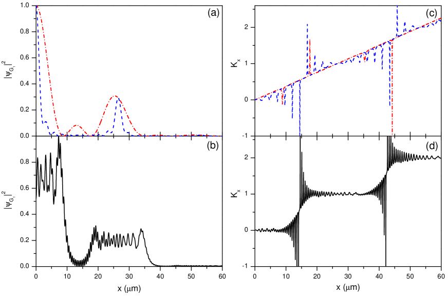
Figure 3: Probability density $|\psi_{G_{1}}(x,z)|^{2}$ (left column) and local transverse momentum $K_{x}$ (right column) evaluated at the position of the grating $G_{2}$ ($z=z_{G_{2}}=0.663$ m) for the same number of slits considered in Fig. 2 and numerically propagated according to Eq. (31). For visual clarity, panels (a) and (c) are for $N=3$ (red dash-dotted line) and $N=11$ (blue dashed line), and panels (b) and (d) for $N=51$. For an easier comparison, in panels (a) and (b) the maximum intensity has been set to one in all cases, while in panels (c) and (d) the momentum is given in units of $2\pi/d$.

We are very familiar with the probability density, but what about the transverse momentum? Does this momentum agree with the assumption that it should be equal to the one carried by each diffraction order? This issue can be easily analyzed by inspecting the right-hand side panels of Fig. 3, where the transverse momentum $K_{x}(x,z_{G_{2}})$ is shown for $N=3$ (red dash-dotted line) and $N=11$ (blue dashed line) in panel (c), and for $N=51$ in panel (d) (again, the graph has been split up for visual clarity). Surprisingly, as seen in panel (c), for low $N$ we find no trace of the momenta related to the diffraction orders, $k_{x,\ell}$. In these cases, $K_{x}$ essentially behaves linearly with the $x$ coordinate in compliance with the relation $K_{x}=(k/z)x$, except at some particular values, where a kind of sudden positive or negative kink is observed. The $x$ values at which this behavior appears are those for which $|\psi_{G_{1}}(x,z_{G_{2}})|^{2}$ vanishes (nodes between maxima). As can be seen, all the spikes that appear in the region from the center of a diffraction order to half the distance between this order and the next one are below the line described by the relation $K_{x}=(k/z)x$; all the spikes in the opposite region are above this line. This indicates a trend: the quantum flux tends to be redirected along the directions of the diffraction orders. Close to the position of the diffraction order, the spikes are relatively weak, while as we move far from it they start increasing. To the left of the diffraction order they are positive, which causes a net effect of pushing the quantum flux towards the right, i.e., approaching it to the position of the diffraction order. On the other hand, as we move to the right of the diffraction order, the spikes increase negatively, pushing the flow leftwards. The combination of both effects leads to an effective confinement or “quantization” of the quantum flux around the corresponding diffraction orders. This becomes more apparent as $N$ gets significantly larger [see panel (d)], when $K_{x}$ starts displaying a staircase structure. This structure corresponds to the momentum quantization associated with the appearance of separated diffraction orders; the emerging well-defined values or steps of (transverse) momenta are precisely $k_{x,\ell}$. This staircase allows us to specifically determine the spatial domain associated with each diffraction order, which has some computational advantages with respect to the numerical simulation of the wave function evolution behind $G_{2}$, as seen below.

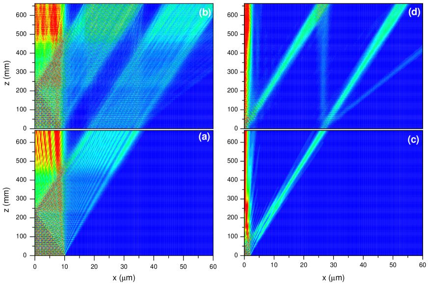
Figure 4: Contour-plots of the probability density between $G_{1}$ and $G_{3}$ for $N=51$ (left) and $N=11$ (right). The evolution of $|\psi_{G_{1}}(x,z)|^{2}$ is displayed in panels (a) and (c) $|\psi_{G_{1}}(x,z)|^{2}$, while $|\psi_{G_{2}}(x,z)|^{2}$ is given in panels (b) and (d). At every value of the $z$-coordinate, the maximum value of the probability density has been set to one; a truncation at 0.8 has then been considered for visual clarity.

The full evolution of the probability density between $G_{1}$ and $G_{3}$ is displayed in Fig. 4 for $N=51$ (left) and $N=11$ (right), respectively, in the form of contour-plots [color scale: maxima are denoted by red, while minima are indicated by blue; because of the faint visibility of the diffraction order $\ell=-1$ in the upper panels (a) and (c), we have introduced a truncation of the maximum contour]. The propagation from $G_{1}$ to $G_{2}$ [see panels (b) and (d)] has been carried out considering that all the slits illuminated contribute with the same weight, while in the transit from $G_{2}$ to $G_{3}$ [see panels (a) and (c)] we have considered $\beta_{j}$ to be proportional to the square root of the probability density reaching $G_{2}$ at the center of the corresponding slit, $j$. In this latter case, if the probability density (normalizing its maximum to unity) was smaller than 0.01, the corresponding $\beta_{j}$ was chosen to be zero. Regarding the momenta $k_{j,x0}$ for the diffracted wave beyond $G_{2}$, we have considered the domains of Fig. 3(d), setting $k_{j,x0}=k_{x,\ell}$ for all $j$ such that $x_{j,0}$ is confined within the region associated with the $\ell$th diffraction order. Given the limited number of Gaussians used to simulate the transit from $G_{2}$ to $G_{3}$ according to the above prescription (329 for $N=51$ and 265 for $N=11$), it has been observed that a direct identification of $k_{j,x0}$ with the local value of $K_{x}$ at $x_{0,j}$ introduces remarkable numerical errors into the simulations due to the fast oscillatory behavior of $K_{x}$ as $N$ increases. This is the reason why this second method to choose $k_{j,x0}$ has been rejected in the current work —although a priori it may seem physically reasonable, it carries computational disadvantages.

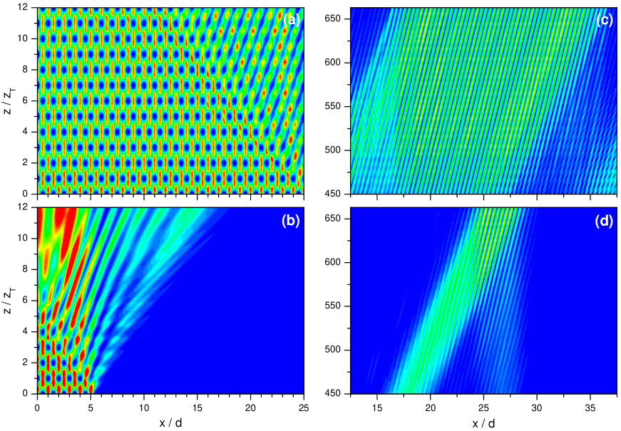
Figure 5: Magnifications to emphasize a series of aspects from Fig. 4. Left: Contour-plots of the probability density $|\psi_{G_{1}}(x,z)|^{2}$ in the near field (close to $G_{1}$) showing the emergence of the Talbot carpet for $N=51$ (a) and $N=11$ (b). Right: Contour-plots of the probability density $|\psi_{G_{2}}(x,z)|^{2}$ in the far field (close to $G_{3}$) for for $N=51$ (c) and $N=11$ (d), where interference features due to the coalescence of the $\ell_{0}=+1$ and $\ell_{+1}=-1$ diffraction orders coalesce around $x=25.42$ $\mu$m are apparent. At every value of the $z$-coordinate, the maximum value of the probability density has been set to one for visual clarity.

The two cases considered in Fig. 4 demonstrate the Mach-Zehnder interferometer configuration formed by the corresponding diffraction orders. Because the diffraction orders are narrower in the case $N=11$, a certain widening is observed from $G_{2}$ to $G_{3}$, as $z$ increases —this behavior is expected from relatively narrow wave packets [33]. Nonetheless, the most relevant aspect, common to both cases, is the relatively complex structure displayed by the wave function along its evolution. Although at a qualitative level one can represent the interferometer in terms of the paths displayed in Fig. 1 (i.e., particle-like behavior), a closer inspection reveals a rather convoluted structure due to the wave nature of the atomic beam all the way through, which cannot be just neglected. In this regard, two structures are worth discussing, namely the near-field carpet that can be seen just behind each grating, and the interference pattern in the far field observable in panels (b) and (d).

The repetitive structures near both $G_{1}$ and $G_{2}$ are associated with a typical effect of periodic gratings on extended waves, namely the so-called Talbot effect [21, 22, 23, 24, 50, 51]. This effect is shown with more detail in the enlargements near $G_{1}$ displayed in the left-hand side panels of Fig. 5. The grating acts on the impinging wave as a collimator that generates a series of identically diffracted waves. The periodicity in the distribution of these waves is such that, if one recast each diffracted wave as a superposition of plane waves, a certain quantization condition arises, which only allows certain momenta [50]. The larger the number of slits the lesser the number of allowed momenta, until reaching a minimum given by the ideal case of $N\to\infty$. Due to this finite basis of momenta, as $z$ increases we observe that the probability density displays recurrences along $x$ within a distance $d$. Thus, at distances $z=2z_{T}=2d^{2}/\lambda=20$ mm we find an exact copy of the initial probability density, where $z_{T}$ is the so-called Talbot distance. Now, because there are no physical boundaries separating different slits, we also find exact copies of the probability density at the Talbot distance, although they have a half a period displacement with respect to the initial pattern. These copies will cover a larger spatial region as $N$ increases, because the basis of momenta will be more limited (compare panels (a) and (b)). Also, if the transmission is different for each slit, we can still observe the Talbot carpet, although with some distortions (see Figs. 4(b) and (d) near $G_{2}$).

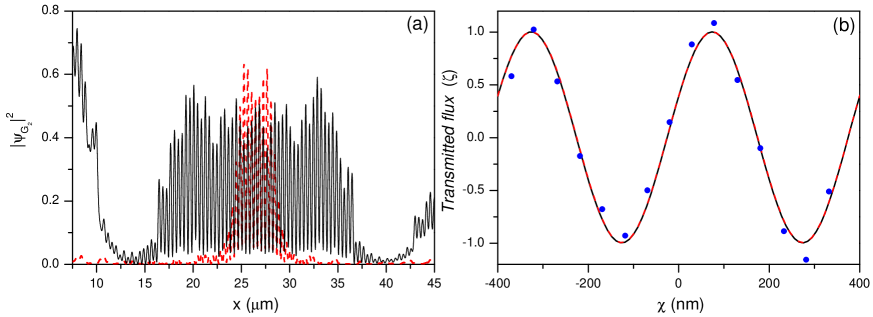
Figure 6: (a) Probability density $|\psi_{G_{2}}(x,z_{G_{2}})|^{2}$ at $G_{3}$ for $N=51$ (black solid line) and $N=11$ (red dashed line). (b) Convolution of the grating transmission function with the intensity around $x_{G_{3}}$, according to Eq. (30). To compare with, the experimental data provided in Ref. [13] are displayed as full (blue) circles. In all cases the transmitted flux is expressed in terms of the normalized function $\zeta$ (see text for details).

In the far field with respect to $G_{2}$, just around $x_{G_{3}}$ at $G_{3}$, we find the the second type of pattern, as can be seen in the right-hand side panels of Fig. 5. Regardless of the number of illuminated slits, this pattern has a period $d$. It is then clear that if $G_{3}$ is gradually moved laterally with respect to this pattern, for some positions the atomic flux passing through the grating will be maximum (in phase), and for other it will be minimum (out of phase), observing a periodic variation (with period $d$), in compliance with Eq. (30). As it was stressed above, the emergence of this pattern is precisely the reason why this peak is important for interferometry: any small perturbation on any of the two paths selected between $G_{1}$ and $G_{2}$ affects its fringe visibility, which can be directly detected through the amount of flux measured behind $G_{3}$. The interference pattern at $G_{3}$ and the amount of transmitted flux as a function of the displacement $\chi$ for $N=51$ and $N=11$ are plotted in Figs. 6(a) and (b), respectively, where the experimental data reported in Ref. [13] are also included (full blue circles in panel (b)). More specifically, in order to avoid contamination from other adjacent diffraction structures, we have performed the convolution integral in both cases within the range between $x=20$ $\mu$m and $x=32.5$ $\mu$m (just around $x_{G_{3}}$), with $\chi$ varying between $-6d$ and $6d$ —in the figure only two periods are shown. In agreement with Eq. (30), the results of panel (b) display the same cosine dependence with $\chi$ in either case, in good agreement with the experimental data reported. Nonetheless, because the total amount of flux collected is larger for $N=51$ than for $N=11$ (the extension covered by the interference pattern is larger), and also for a better comparison with the experimental data, instead of directly plotting Eq. (30), we have considered the normalized function

$$\zeta=\frac{\mathcal{T}_{G_{3}}(\chi)-\bar{\mathcal{T}}_{G_{3}}}{\Delta\mathcal{T}_{G_{3}}},$$ (36)

where $\bar{\mathcal{T}}_{G_{3}}=(\mathcal{T}_{G_{3}}^{\rm max}+\mathcal{T}_{G_{3}}^{\rm min})/2$ and $\Delta\mathcal{T}_{G_{3}}=(\mathcal{T}_{G_{3}}^{\rm max}-\mathcal{T}_{G_{3}}^{\rm min})/2$. Moreover, the maxima of the numerical calculations have also been shifted in order to align them with those of the experimental data. Nonetheless, unlike the models considered in the literature, we would like to highlight that here no best-fit procedure has been used in any of the steps to adjust our results to the reported experimental data; the agreement between our simulations and the experiment directly arises from the few working hypotheses considered above.

5 Concluding remarks

We have shown that by using the relationship between the configuration and momentum representations of a wave function it is possible a simple analysis of atomic three-grating Mach-Zehnder interferometers. This analysis shows how three gratings behave in the same way as the set of two beam-splitters and two mirrors does in conventional optical Mach-Zehnder interferometers. As a convenient working model we have considered a Gaussian grating given its analytical and computational advantages. On the one hand, this type of grating has allowed us to obtain a series of analytical expansions and results in the far field, which can be readily compared to the experiment, providing us with an important physical insight on the interferometers here considered. On the other hand, the fact that the time-evolution of Gaussian wave packets (or, equivalently, their propagation along the longitudinal direction) is fully analytical, also constitutes a remarkable simplification in the design of simple numerical codes that allow to compute the probability density or the local transverse momentum at any intermediate step between two consecutive gratings. In this regard, the local transverse momentum has been introduced as an important analytical tool, borrowed from the Bohmian formulation of quantum mechanics and related to the usual flux operator. Based on this working model, a reasonable ansatz for the passage through the second grating can also be easily proposed, without any need to use more complex and higher time-consuming wave-packet propagation techniques [32], where the presence of gratings is usually introduced in terms of interaction potentials [34].

The information obtained from the analytical and numerical results not only complements each other, but is very valuable to understand different aspects of how atomic three-grating Mach-Zehnder interferometers work. From experimental data, the analytical results have shown in a simple manner how the two branches of the interferometer appear as well as how, later on, they coalesce and give rise to an interference structure with the same period of the gratings. In particular, first one readily notices that because the diffraction orders are well separated spatially, one can work with only two of them, neglecting other contributions. This fact relies on the property that only the probability along the diffraction orders $\ell=0$ and $\pm 1$ is physically relevant. This has been confirmed by the numerical simulations. In spite of the rather complex evolution displayed by the wave function between consecutive gratings, particularly in the corresponding near field regions, in practice this does not count much, this showing the correctness of oversimplified sketches like the one displayed in Fig. 1. Hence, bringing back the old wave-corpuscle dichotomy, we have shown that wave and particle are not incompatible aspects, but the misuse that we typically do of them to explain and understand these experiments. The incident atomic beam behaves as a wave all the way through, although in the transit one can simplify the picture by assuming that the atoms behave as classical point-like particles moving along straight lines. Of course, this is done at the expense of neglecting the rich interference structures that arise along the way.

From a practical viewpoint, we would also like to highlight the fact that the simplicity of the model here considered makes feasible the analysis of incoherence due to a lack of full periodicity in the gratings, presence of thermal vibrations, or decoherence by an external environment in a simple manner. This can be done by playing around with the different parameters associated with the Gaussians as well as with the way how the latter overlap. Indeed, both the model and the methodology here developed are not constrained to the system that we have analyzed, but they can be easily and conveniently implemented in other experimental contexts due to their versatility. Notice that, generally speaking, the main purpose of this work consists in providing a clear, precise and simple methodology (working model) to simulate, analyze, understand and explain interference processes and interferometry experiments. This is something in the borderline between the simplistic approaches often considered in the literature (which always require of fitting parameters and do not account for the full dynamical process that takes place inside the interferometer), and tough and serious (very realistic) quantum-dynamical calculations implying determining the potential energy surfaces associated with the interaction between the diffracted particles and the diffracting gratings as a function of the distance (e.g., atom-atom, atom-molecule or molecule-molecule scattering processes). In a few words, by means of this procedure we have tried to make quantum mechanics less mystic, showing that a relatively complex dynamical process can be easily explained by means of a few working hypotheses and a simple model.

References

- [1] G. Badurek, H. Rauch, A. Zeilinger (Eds.), Proceedings of the International Workshop on Matter Wave Interferometry (Vienna 1987), Physica B 151 (1988) 3-400.
- [2] C.S. Adams, M. Sigel, J. Mlynek, Atom optics, Phys. Rep. 240 (1994) 143–210.
- [3] P. Berman, Atom Interferometry, Academic Press, San Diego, 1997.
- [4] A.D. Cronin, J. Schmiedmayer, D.E. Pritchard, Optics and interferometry with atoms and molecules, Rev. Mod. Phys. 81 (2009) 1051–1129.
- [5] M. Arndt, K. Hornberger, Quantum Interferometry with Complex Molecules, in Proceedings of the International School of Physics “Enrico Fermi”, Course CLXXI “Quantum Coherence in Solid State Systems”, P. Schwendimann (Ed.), Societá Italiana di Fisica, 2008.
- [6] M. Arndt, A. Ekers, W. von Klitzing, H. Ulbricht, Focus on modern frontiers of matte wave optics and interferometry, New J. Phys. 14 (2012) 125006(1-9).
- [7] M. Kasevich, S. Chu, Atomic interferometry using stimulated Raman transitions, Phys. Rev. Lett. 67 (1991) 181–184.
- [8] I. Estermann, O. Stern, Beugung von Molekularstrahlen, Z. Physik 61 (1930) 95–125.
- [9] P.L. Gould, G.A. Ruff, D.E. Pritchard, Diffraction of atoms by light: The near-resonant Kapitza-Dirac effect, Phys. Rev. Lett. 56 (1986) 827–830.
- [10] P.L. Kapitza, P.A.M. Dirac, The reflection of electrons from standing light waves, Proc. Cambridge Phil. Soc. 29 (1933) 297–300.
- [11] D.L. Freimund, K. Aflatooni, H. Batelaan, Observation of the Kapitza-Dirac effect, Nature 413 (2001) 142–143.
- [12] D.W. Keith, M.L. Schattenburg, H.I. Smith, D.E. Pritchard, Diffraction of atoms by a transmission grating, Phys. Rev. Lett. 61 (1988) 1580–1583.
- [13] D.W. Keith, C.R. Ekstrom, Q.A. Turchette, D.E. Pritchard, An interferometer for atoms, Phys. Rev. Lett. 66 (1991) 2693–2696.
- [14] E.M. Rasel, M.K. Oberthaler, H. Batelaan, J. Schmiedmayer, A. Zeilinger, Atom wave interferometry with diffraction gratings of light, Phys. Rev. Lett. 75 (1995) 2633–2637.
- [15] O. Carnal, A. Faulstich, J. Mlynek, Diffraction of metastable helium atoms by a transmission grating, Appl. Phys. B 53 (1991) 88–91.
- [16] B. Brezger, L. Hackermüller, S. Uttenthaler, J. Petschinka, M. Arndt, A. Zeilinger, Matter-wave interferometer for large molecules, Phys. Rev. Lett. 88 (2002) 100404(1–4).
- [17] K. Hornberger, S. Gerlich, P. Haslinger, S. Nimmrichter, M. Arndt, Colloquium: Quantum interference of clusters and molecules, Rev. Mod. Phys. 84 (2012) 157–173.
- [18] T. Juffmann, A. Milic, M. Müllneritsch, P. Asenbaum, A. Tsukernik, J. Tüxen, M. Mayor, O. Cheshnovsky, M. Arndt, Real-time single-molecule imaging of quantum interference, Nat. Nanotech. 7 (2012) 297–300.
- [19] J.F. Clauser, S. Li, Talbot-vonLau atom interferometry with cold slow potassium, Phys. Rev. A 49 (1994) R2213–R2216.
- [20] J.F. Clauser, M.W. Reinsch, New theoretical and experimental results in Fresnel optics with applications to matter-wave and X-ray interferometry, Appl. Phys. B 54 (1992) 380–395.
- [21] H.F. Talbot, Facts relating to optical science, Phil. Mag. 9 (1836) 401–407.
- [22] L. Rayleigh, On copying diffraction-gratings, and some phenomena connected therewith, Philos. Mag. 11 (1881) 196–205.
- [23] J.T. Winthrop, C.R. Worthington, Theory of Fresnel Images. I. Plane periodic objects in monochromatic light. J. Opt. Soc. Am. 55 (1965) 373–381.
- [24] P. Latimer, R.F. Crouse, Talbot effect reinterpreted, Appl. Opt. 31 (1992) 80–89.
- [25] E. Lau, Beugungserscheinungen an Doppelrastern, Ann. Phys. 6 (1948) 417–423.
- [26] J. Jahns, A.W. Lohmann, The Lau effect: A diffraction experiment with incoherent illumination, Opt. Commun. 28 (1979) 263–267.
- [27] R. Sudol, B.J. Thompson, Lau effect: Theory and experiment, Appl. Opt. 20 (1981) 1107–1116.
- [28] P. Storey, C. Cohen-Tannoudji, The Feynman path integral approach to atomic interferometry. A tutorial, J. Phys. II France 4 (1994) 1999–2027.
- [29] P. Nachman, Mach-Zehnder interferometry as an instructional tool, Am. J. Phys. 63 (1995) 39–43.
- [30] A.S. Sanz, S. Miret-Artés, A Trajectory Description of Quantum Processes. I. Fundamentals, Springer, Berlin, 2012.
- [31] L.I. Schiff, Quantum Mechanics, McGraw-Hill, Singapore, 1968.
- [32] J.Z.H. Zhang, Theory and Application of Quantum Molecular Dynamics, World Scientific, Singapore, 1999.
- [33] A.S. Sanz, S. Miret-Artés, A trajectory-based understanding of quantum interference, J. Phys. A 41 (2008) 435303(1-23).
- [34] A.S. Sanz, S. Miret-Artés, Atom-surface diffraction: A quantum trajectory description, in Quantum Dynamics of Complex Molecular Systems, D.A. Micha and I. Burghardt (Eds.), Springer, Berlin, 2006, pp. 343–368.
- [35] R. Gelabert, X. Giménez, M. Thoss, H. Wang, W. H. Miller, Semiclassical description of diffraction and its quenching by the forward-backward version of the initial value representation, J. Chem. Phys. 114 (2001) 2572–2579.
- [36] R.E. Grisenti, W. Schöllkopf, J.P. Toennies, G.C. Hegerfeldt, T. Köhler, Determination of atom-surface van der Waals potential from transmission-grating diffraction intensities, Phys. Rev. Lett. 83 (1999) 1755–1758.
- [37] R.E. Grisenti, W. Schöllkopf, J.P. Toennies, J.R. Manson, T.A. Savas, H.I. Smith, He-atom diffraction from nanostructure transmission gratings: The role of imperfections, Phys. Rev. A 61 (2000) 033608(1–15).
- [38] R. P. Feynman and A. R. Hibbs, Quantum Mechanics and Path Integrals, McGraw-Hill, New York, 1965. Emended version: R. P. Feynman, A. R. Hibbs, D. F. Styer, Quantum Mechanics and Path Integrals, Dover, New York, 2010.
- [39] M. Božić, D. Arsenović, A.S. Sanz, M. Davidović, On the influence of resonance photon scattering on atom interference, Phys. Scr. T140 (2010) 014017(1–5).
- [40] L.E. Ballentine, Quantum Mechanics: A Modern Development, World Scientific, Singapore, 1998.
- [41] M. Božić, D. Dimić, M. Davidović, Coherent beam splitting by a thin grating, Acta Phys. Pol. A 116 (2009) 479–482.
- [42] A. Lipson, S.G. Lipson, H. Lipson, Optical Physics, Cambridge University Press, Cambridge, 2011, 4th Ed.
- [43] E. Hecht, Optics, Addison-Wesley Longman, New York, 2002, 4th Ed.
- [44] A.S. Sanz, F. Borondo, and S. Miret-Artés, “Particle diffraction studied using quantum trajectories,” J. Phys.: Condens. Matter 14, 6109-6145 (2002).
-
[45]
This can be easily shown by taking into account the relations:
with .(39) (42) - [46] O. Carnal, J. Mlynek, Young’s double-slit experiment with atoms: A simple atom interferometer. Phys. Rev. Lett. 66 (1991) 2689–2692.
- [47] M.S. Chapman, T.D. Hammond, A. Lenef, J. Schmiedmayer, R.A. Rubenstein, E. Smith, D.E. Pritchard, Photon scattering from atoms in an atom interferometer: Coherence lost and regained, Phys. Rev. Lett. 75 (1995) 3783–3787.
- [48] M. Davidović, A.S. Sanz, M. Božić, D. Arsenović, Coherence loss and revivals in atomic interferometry: A quantum-recoil analysis, J. Phys. A 45 (2012) 165303(1–17).
- [49] A.S. Sanz, S. Miret-Artés, A Trajectory Description of Quantum Processes. II. Applications, Springer, Berlin, 2014.
- [50] A.S. Sanz, S. Miret-Artés, A causal look into the quantum Talbot effect, J. Chem. Phys. 126 (2007) 234106(1–11).
- [51] M. Davidović, D. Arsenović, M. Božić, A.S. Sanz, S. Miret-Artés, Should particle trajectories comply with the transverse momentum distribution?, Eur. Phys. J.-Spec. Top. 160 (2008) 95–104.