Map-Aware Models for Indoor Wireless Localization Systems: An Experimental Study

Abstract

The accuracy of indoor wireless localization systems can be substantially enhanced by map-awareness, i.e., by the knowledge of the map of the environment in which localization signals are acquired. In fact, this knowledge can be exploited to cancel out, at least to some extent, the signal degradation due to propagation through physical obstructions, i.e., to the so called non-line-of-sight bias. This result can be achieved by developing novel localization techniques that rely on proper map-aware statistical modelling of the measurements they process. In this manuscript a unified statistical model for the measurements acquired in map-aware localization systems based on time-of-arrival and received signal strength techniques is developed and its experimental validation is illustrated. Finally, the accuracy of the proposed map-aware model is assessed and compared with that offered by its map-unaware counterparts. Our numerical results show that, when the quality of acquired measurements is poor, map-aware modelling can enhance localization accuracy by up to 110% in certain scenarios.

I Introduction

In recent years significant attention has been devoted to the development of accurate and low cost wireless localization systems for indoor civilian applications, since they can be employed to provide a number of new services, like asset tracking and tracking of people with special needs [1, 2]. In these services estimated positions need always to be related to a surrounding infrastructure (e.g., rooms and corridors) to be useful to their end users, so that the knowledge of the map of the environment where users are expected to move (e.g., the plan of a building floor) is required. In principle, map knowledge (i.e., map-awareness) can be also exploited to improve the estimation accuracy of a localization system. In fact, any wireless localization system first acquires a set of point-to-point measurements related to user position (first step; technology-dependent) and then processes such measurements for bi-dimensional (2-D) or three-dimensional position estimation by means of a proper localization technique (second step; technology-agnostic) [3, Sec. 4]. Maps can play a significant role in the second step, since they provide information about environmental obstructions (e.g., walls) which interfere with signal propagation; however, a full exploitation of these information requires a) the availability of map-aware statistical models for the acquired measurements and b) the development of localization techniques explicitly based on these models.

At present the only available map-aware statistical models are the wall extra delay (WED) model [4, eq. (6)] and the attenuation factor (AF) model [5, Sec. 4.11.5] (also known as wall-attenuation model or multi-wall model [6]); these models have been developed for time of arrival (TOA) and received signal strength (RSS) localization systems, respectively, and are based on experimental evidence. This preliminary work shows that map-awareness can significantly improve localization accuracy by compensating for the so called non-line-of-sight (NLOS) bias, which is a major source of error. However, as far as we know, the accuracy and validity of the above mentioned models in real world localization systems is under-explored and, generally speaking, there is a lack of experimental results supporting them in the technical literature. In fact, most of the state-of-the-art localization methods rely on map-unaware models. For instance, the well known log-distance propagation model [1, 7, 8, 9, 10, 5] (or, in some cases, models based on polynomial series expansions [11]) are adopted to relate RSS to distance. Similar comments hold for those models relating TOA and time difference of arrival (TDOA) to distance; in this case additive error terms are usually represented by Gaussian random variables (rvs) [1, eq. (6)], [12, 13, 14], although more refined models accounting for NLOS propagation are also available (see [15, 16] and references therein).

It is also worth mentioning that map-awareness is implicitly employed in fingerprinting-based localization systems to select fingerprint locations [17, 18, 19]. In those systems no statistical modelling of acquired measurements is needed (even if combined fingerprinting/statistical approaches are possible [20]); however, extensive and time consuming measurement campaigns (which may be very sensitive to environmental changes) are necessary to achieve an acceptable accuracy, since the localization error of fingerprinting methods is roughly bounded by the spacing between calibration sites.

The aim of this manuscript is twofold. First of all, a novel unified statistical map-aware model for TOA, TDOA or RSS measurements is proposed and is validated exploiting a set of RSS and ultra wide band (UWB) TOA data acquired in indoor environments. Secondly, the improvement in localization accuracy provided by optimal localization algorithms based on the novel map-aware modelling with respect to their counterparts relying on map-unaware modelling is quantified; this unveils that, specially in RSS systems, the accuracy improvement justifies the increased complexity of map-aware modelling.

The proposed map-aware model has the following relevant features: a) it relates the NLOS bias affecting measurements to map geometrical features; b) it can be employed in localization systems based on ranging techniques (i.e., TOA, TDOA and RSS, but not angle of arrival [21, 3]) provided that their radio signals mainly propagate through obstructions; c) it contains few parameters to be estimated from measurements; d) even if its validity is assessed for narrowband low-frequency RSS measurements and for TOA UWB measurements, its use can be envisaged for other technologies, like wireless local area network TOA/TDOA or even non-radio-based technologies (e.g, ultra-sound), since it does not rely on technology-specific properties; e) likelihood functions based on it can be employed in navigation systems (where mobile agents are considered).

This manuscript is organized as follows. In Section II, the localization system we consider is described and general statistical models for map-aware and map-unaware scenarios are proposed. Specific models for RSS and TOA measurements, based on our experimental data, are illustrated in Section III. In Section IV map-aware and map-unaware optimal localization algorithms are derived, their performance is assessed and compared, and some indications about their computational complexity are provided. Finally, Section V offers some conclusions.

Notations: The probability density function (pdf) of the rv $R$ evaluated at the point $r$ is denoted $f(r)$; $\mathcal{N}\left(r;\mu,\sigma^{2}\right)$ denotes the pdf of a Gaussian rv having mean $\mu$ and variance $\sigma^{2}$, evaluated at the point $r$; $\mathcal{E}\left(r;t,\mu\right)$ denotes the pdf of an exponential rv translated by $t$ and having mean $t+\mu$, evaluated at the point $r$, so that $\mathcal{E}\left(r;t,\mu\right)\triangleq\frac{1}{\mu}\exp\left(\frac{t-r}{\mu}\right)\operatorname{u}(r-t)$, where $\operatorname{u}(x)$ denotes the Heaviside step function; $\left|\mathcal{S}\right|$ denotes the cardinality of the set $\mathcal{S}$ ;$\left\lfloor x\right\rfloor$ denotes the floor of the real parameter $x$; $\star$ denotes the convolution integral.

II Modelling of Reference Scenario

Figure 1: Example of a localization system employing $N_{a}=6$ anchors (green squares) to localise a single agent (blue circle) and operating over a bounded map (whose support $\mathcal{R}$ is identified by the grey area). The presence of a LOS (NLOS) link between the agent and a given anchor is evidenced by a continuous (dashed) line (note that propagation conditions prevent establishing a wireless link between the agent and the anchors 4 and 5).

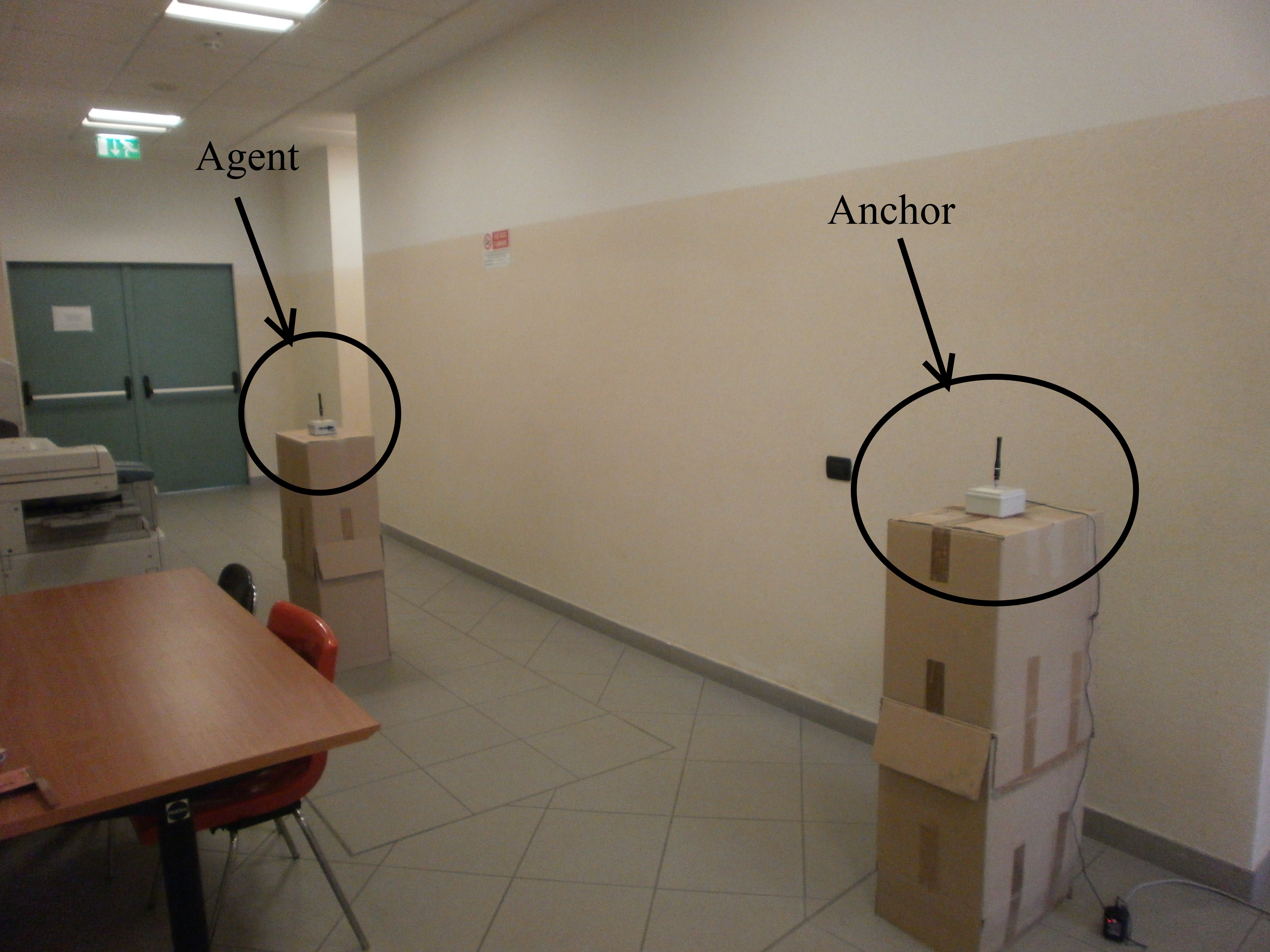
In the following we focus on a 2-D localization system operating in an indoor scenario and employing $N_{a}$ devices, called anchors and whose positions $\left\{\mathbf{p}_{i}^{a}\right\}_{i=1}^{N_{a}}$ are known, to estimate the position $\mathbf{p}$ of a single agent in a large indoor scenario (i.e., the floor of a large building). The system structure is exemplified by Fig. 1 for $N_{a}=6$. Formulating the problem of map-aware localization requires defining mathematical models for a) its map, b) the wireless connectivity between the agent and the anchors, and c) the measurements acquired for position estimation. These models are illustrated in the following three paragraphs.

II-A Map Model

Our prior knowledge about the agent position $\mathbf{p}\triangleq\left[x,y\right]^{T}$ is expressed by the uniform pdf [22]

$$f(\mathbf{p})=\begin{cases}1/\mathcal{A_{R}}&\mathbf{p}\in\mathcal{R}\\ 0&\text{elsewhere}\end{cases}$$ (1)

where $\mathcal{R}\subset\mathbb{R}^{2}$ denotes the region where the agent is constrained to lie and $\mathcal{A}_{\mathcal{R}}$ its area. Note that (1) describes a uniform map model, which is fully characterized by the map support $\mathcal{R}$ (whose bounding box is $\mathcal{B}\left(\mathcal{R}\right)$). In the following we assume that any map-aware (map-unaware) localization system is endowed with the knowledge of $\mathcal{R}$ ($\mathcal{B}\left(\mathcal{R}\right)$). Note that the propagation of wireless signals (and, consequently, localization performance) is affected by the obstructions (e.g., walls) shaping the map support $\mathcal{R}$; in particular, an important role is played by the number of obstructions $N_{o}\left(\mathbf{p}_{1},\mathbf{p}_{2}\right)$ interposed between two arbitrary points $\mathbf{p}_{1}$ and $\mathbf{p}_{2}$, both belonging to $\mathcal{R}$.

II-B Connectivity Model

We assume that an agent located at $\mathbf{p}$ is connected with the $i$-th anchor when the signal-to-noise ratio (SNR) of the wireless signal radiated by this anchor and received by the agent exceeds a given threshold (i.e., the agent’s receiver sensitivity); therefore, each anchor is characterized by a specific coverage region. Even if the map of the environment is known, the prediction of the shape of each coverage region is not easy. For this reason, the following simple (map-unaware) connectivity model is adopted: the coverage region $\mathcal{R}^{(i)}$ of the $i$-th anchor is a circle centered at $\mathbf{p}_{i}^{a}$ and whose radius $d_{\text{\tiny{max}},i}$ depends on the power radiated by the anchor itself and the propagation conditions. Then, the signal coming from the $i$-th anchor is theoretically detectable inside $\mathcal{R}^{(i)}$ and in such a region some localization information or, more precisely, an observation (denoted $z_{i}$) can be acquired in the first step of any localization technique (see Section I).

In practice, in the presence of harsh propagation conditions the number $N_{obs}$ of observations available to the agent may differ from the number which can be predicted theoretically using the above mentioned connectivity model. Let $\mathcal{Z}$ denote the set of indices associated with the anchors truly connected with the agent; then, we have that $N_{obs}\triangleq\left|\mathcal{Z}\right|$ and that, if $i\in\mathcal{Z}$, then $\mathbf{p}\in\mathcal{R}^{(i)}\bigcap\mathcal{R}$. Consequently, in a map-aware localization system the agent position has to be searched for inside the region

$$\mathcal{R}^{(\mathcal{Z})}\triangleq\left(\bigcap_{i\in\mathcal{Z}}\mathcal{R}^{(i)}\right)\bigcap\mathcal{R}$$ (2)

whereas, in a map-unaware system, the agent position is expected to belong to

$$\mathcal{P}^{(\mathcal{Z})}\triangleq\left(\bigcap_{i\in\mathcal{Z}}\mathcal{R}^{(i)}\right)\bigcap\mathcal{B}\left(\mathcal{R}\right)$$ (3)

Finally, it is important to note that the wireless links referring to the anchors connected with an agent located at $\mathbf{p}$ can be in line of sight (LOS) or NLOS conditions. For this reason, the set $\mathcal{Z}$ can be partitioned into the subsets $\mathcal{Z}^{\text{\tiny{LOS}}}\triangleq\left\{i\in\mathcal{Z}|N_{o}\left(\mathbf{p},\mathbf{p}_{i}^{a}\right)=0\right\}$ and $\mathcal{Z}^{\text{\tiny{NLOS}}}\triangleq\mathcal{Z}/\mathcal{Z}^{\text{\tiny{LOS}}}$ containing the indices of the connected anchors in LOS and NLOS conditions, respectively.

II-C Observation Model

The localization system we consider statistically infers the agent position $\mathbf{p}$ from a set of $N_{obs}$ observations (in practice, estimated ranges) $\left\{z_{i},i\in\mathcal{Z}\right\}$ extracted from the radio signals coming from the connected anchors. For an indoor environment, such signals are affected by multipath fading [5, Sec. 5] which substantially complicates the problem of the statistical modelling of the available observations. To simplify this problem, we assume that: a) the time interval needed to acquire all the observations is small with respect to the coherence time of the propagation scenario, so that the effects due to its time selectivity can be ignored; b) in TOA-based systems the effects due to the time dispersion characterising the propagation scenario are mitigated transmitting wideband signals, so that multiple echoes of the signal radiated by a given anchor can be resolved by the agent (in particular, the first path can be correctly detected). Given such assumptions, the observation model

$$z_{i}=d_{i}(\mathbf{p})+b_{i}(\mathbf{p})+n_{i}(\mathbf{p})$$ (4)

characterized by additive bias and noise terms and commonly adopted in the localization literature (e.g., see [4, Eq. (3)], [9] and [13, Eq. (3)] ) can be also employed in our scenario for any $i\in\mathcal{Z}$; here $d_{i}(\mathbf{p})\triangleq\left\|\mathbf{p}-\mathbf{p}_{i}^{a}\right\|$ denotes the true distance between the agent position $\mathbf{p}$ and the $i$-th anchor, $b_{i}(\mathbf{p})$ represents the NLOS bias originating from obstructions affecting the $i$-th wireless link and $n_{i}(\mathbf{p})\sim\mathcal{N}(0,\sigma_{n,i}^{2}(\mathbf{p}))$ is a noise term modelling various sources of errors (e.g., the error introduced in extrapolating the observation $z_{i}$ from the continuous-time waveform collected by the agent antenna, the radio interference, and the noise generated by both transmitter and receiver hardware). It is important to point out that:

1. The effects of spatial selectivity (that may generate substantial fluctuations in the received power as the agent position changes) are difficult to predict and hence have been included in the noise term $n_{i}(\mathbf{p})$, even if the availability of a simple and reliable model for spatial fading would certainly improve model accuracy.

2. The $i$-th observation $z_{i}$ (4) is generated by mapping, through a function denoted $\psi(\cdot)$ in the following, the physical quantity measured by the hardware (e.g., a RSS or a TOA) into a range. The function $\psi(\cdot)$ is derived under the assumption of LOS propagation, since NLOS propagation conditions are accounted for by introducing the bias term $b_{i}(\mathbf{p})$ in (4). In map-aware modelling such a term is modelled as $b_{i}(\mathbf{p})\sim\mathcal{N}(\mu_{b,i}(\mathbf{p}),\sigma_{b,i}^{2}(\mathbf{p}))$ for $i\in\mathcal{Z}^{\text{\tiny{NLOS}}}$ and $b_{i}(\mathbf{p})=0$ for $i\in\mathcal{Z}^{\text{\tiny{LOS}}}$; a different (and not necessarily Gaussian) model is adopted, instead, in map-unaware modelling, as discussed in detail below.

Providing further details about the observation model (4) requires a) considering specific localization techniques (in the following, quantities specifically referring to TOA and RSS techniques are identified by the superscripts ${}^{\text{\tiny{TOA}}}$ and ${}^{\text{\tiny{RSS}}}$, respectively) and b) making a clear distinction between map-aware and map-unaware modelling, as illustrated below.

TOA-based localization - In this case the observation $z_{i}$ is related to the measured TOA $\tau_{i}$ (expressed in seconds) by the LOS mapping $z_{i}^{\text{\tiny{TOA}}}=\psi^{\text{\tiny{TOA}}}(\tau_{i})=c_{0}\tau_{i}$, where $c_{0}$ is the speed of light in vacuum. In NLOS propagation conditions $z_{i}^{\text{\tiny{TOA}}}$ is affected by a bias (due to the fact that obstacles slow down electromagnetic waves); in map-aware systems, the NLOS bias mean $\mu_{b,i}^{\text{\tiny{TOA}}}(\mathbf{p})$ can be modelled as [4, Sec. 3.3.1]

$$\mu_{b,i}^{\text{\tiny{TOA}}}(\mathbf{p})=\sum_{j=1}^{N_{o}\left(\mathbf{p},\mathbf{p}_{i}^{a}\right)}t_{w,j}\sqrt{\epsilon_{r,w,j}-1}$$ (5)

for any $i\in\mathcal{Z}$, where $t_{w,j}$ and $\epsilon_{r,w,j}$ are the thickness and the relative electrical permittivity, respectively, of the $j$-th obstruction. If all the obstructions have the same thickness $t_{w}$ and the same permittivity $\epsilon_{r,w}$, (5) simplifies as $\mu_{b,i}^{\text{\tiny{TOA}}}(\mathbf{p})=N_{o}\left(\mathbf{p},\mathbf{p}_{i}^{a}\right)\cdot t_{w}\sqrt{\epsilon_{r,w}-1}$ [4, Eq. (6)]. In map-unaware localization systems, instead, we assume that: a) a state-of-the-art localization strategy relying on a LOS/NLOS detector is adopted ; b) such a detector is characterized by an error (i.e., false detection and missed detection) probability $P_{e}^{\text{\tiny{NLOS}}}$ over each link; c) it provides the map-unaware localization algorithm with the estimates $\hat{\mathcal{Z}}^{\text{\tiny{LOS}}}$ and $\hat{\mathcal{Z}}^{\text{\tiny{NLOS}}}$ of the sets $\mathcal{Z}^{\text{\tiny{LOS}}}$ and $\mathcal{Z}^{\text{\tiny{NLOS}}}$, respectively. Given these estimates, the model $b_{i}^{\text{\tiny{TOA}}}(\mathbf{p})\sim\mathcal{E}(0,\nu_{b}^{\text{\tiny{TOA}}})$ is employed for any $i\in\hat{\mathcal{Z}}^{\text{\tiny{NLOS}}}$, since the NLOS bias is always positive for TOA measurements [13, 14, 23].

TDOA-based localization - The results illustrated above for TOA modelling can be easily exploited for TDOA-based localization systems. In fact, in this case $z_{i}$ is evaluated subtracting the TOA provided by a reference anchor from that acquired by the $i$-th anchor and both measurements are modelled by (4); further details are not provided here for space limitations.

RSS-based localization - In this case the observation $z_{i}$ is related to the measured RSS $P_{rx,i}$ (i.e., the average power of the radio signal received by the agent from the $i$-th anchor) according to the formula $z_{i}^{\text{\tiny{RSS}}}=\psi^{\text{\tiny{RSS}}}(P_{rx,i})$; specific forms for $\psi^{\text{\tiny{RSS}}}(\cdot)$ are discussed later in Sec. III-A. NLOS propagation needs to be accounted for carefully in RSS-based systems, since the attenuation due to obstructions results in an overestimated range $z_{i}^{\text{\tiny{RSS}}}$. However, unlike the TOA and TDOA cases, no simple and accurate theoretical formula is available to model the NLOS bias mean in map-aware localization, so that models extracted from experimental data must be employed. In our work measurement-based models have been developed for both $\mu_{b,i}^{\text{\tiny{RSS}}}(\mathbf{p})$ and $\sigma_{b,i}^{\text{\tiny{RSS}}}(\mathbf{p})$ (see Section III); such models are similar to the experimental AF model (developed in [5, Sec. 4.11.5] and assuming a logarithmic dependence of the RSS on the number of obstructions). In the map-unaware case, instead, we assume again the availability of a LOS/NLOS detector characterized by the error probability $P_{e}^{\text{\tiny{NLOS}}}$ and adopt the bias model $b_{i}^{\text{\tiny{RSS}}}(\mathbf{p})\sim\mathcal{N}(\kappa_{b}^{\text{\tiny{RSS}}},\gamma_{b}^{\text{\tiny{RSS}}})$.

The statistical models illustrated above allow us to develop a novel unified (i.e., valid for TOA, TDOA and RSS) statistical representation for the set of observations $\left\{z_{i},i\in\mathcal{Z}\right\}$. In fact, given the trial agent position $\tilde{\mathbf{p}}\in\mathcal{R}^{(\mathcal{Z})}$, the map-aware likelihood associated with these observations can be expressed as (see (4))

$$f(\mathbf{z}|\tilde{\mathbf{p}})=\prod_{i\in\mathcal{Z}}\mathcal{N}\left(z_{i};d_{i}(\tilde{\mathbf{p}})+\mu_{b,i}(\tilde{\mathbf{p}}),\sigma_{n,i}^{2}(\tilde{\mathbf{p}})+\sigma_{b,i}^{2}(\tilde{\mathbf{p}})\right)$$ (6)

where $\mathbf{z}\triangleq\left[z_{i},\forall i\in\mathcal{Z}\right]^{T}$. Similarly, the map-unaware counterpart of (6), given the trial agent position $\tilde{\mathbf{p}}\in\mathcal{P}^{(\mathcal{Z})}$, can be put in the form

$$f(\mathbf{z};\tilde{\mathbf{p}})= \prod_{i\in\hat{\mathcal{Z}}^{\text{\tiny{LOS}}}}\mathcal{N}\left(z_{i};d_{i}(\tilde{\mathbf{p}}),\sigma_{n,i}^{2}(\tilde{\mathbf{p}})\right)$$

$$\prod_{i\in\hat{\mathcal{Z}}^{\text{\tiny{NLOS}}}}\mathcal{N}\left(z_{i};d_{i}(\tilde{\mathbf{p}})+\kappa_{b},\sigma_{n,i}^{2}(\tilde{\mathbf{p}})+\gamma_{b}^{2}\right)$$ (7)

or

$$f(\mathbf{z};\tilde{\mathbf{p}})= \prod_{i\in\hat{\mathcal{Z}}^{\text{\tiny{LOS}}}}\mathcal{N}\left(z_{i};d_{i}(\tilde{\mathbf{p}}),\sigma_{n,i}^{2}(\tilde{\mathbf{p}})\right)$$

$$\prod_{i\in\hat{\mathcal{Z}}^{\text{\tiny{NLOS}}}}\left[\mathcal{E}\left(z_{i};0,\nu_{b}\right)\star\mathcal{N}\left(z_{i};d_{i}(\tilde{\mathbf{p}}),\sigma_{n,i}^{2}(\tilde{\mathbf{p}})\right)\right]$$ (8)

if a Gaussian or an exponential model is adopted for the NLOS bias, respectively. In the latter case, the convolution integral appearing in the right-hand side of (8) substantially complicates the likelihood (8); for this reason in the technical literature (e.g., see [23]) it is usually assumed that the NLOS bias dominates over the Gaussian noise, so that (8) can be approximated as

$$f(\mathbf{z};\tilde{\mathbf{p}})\simeq \prod_{i\in\hat{\mathcal{Z}}^{\text{\tiny{LOS}}}}\mathcal{N}\left(z_{i};d_{i}(\tilde{\mathbf{p}}),\sigma_{n,i}^{2}(\tilde{\mathbf{p}})\right)\prod_{i\in\hat{\mathcal{Z}}^{\text{\tiny{NLOS}}}}\mathcal{E}\left(z_{i};d_{i}(\tilde{\mathbf{p}}),\nu_{b}\right).$$ (9)

Finally, it is important to stress that (6) and (7)-(9) represent general statistical models applying to TOA, TDOA and RSS measurements (under the assumptions described above); in the next Section they will be specialized to fit our experimental results.

III Extraction of Model Parameters From Experimental Results

In this Section we provide a) various details about the measurement campaigns supporting our proposed models, b) some explicit expressions for the functions $\psi^{\text{\tiny{RSS}}}(\cdot)$, $\mu_{b,i}^{\text{\tiny{RSS}}}(\mathbf{p})$, $\sigma_{b,i}^{2}(\mathbf{p})$ and $\sigma_{n,i}^{2}(\mathbf{p})$, and c) the exact form of the likelihood functions fitting our experimental data.

III-A RSS Measurement Campaign

RSS data have been acquired in a measurement campaign performed by our research group in the first half of 2012. Two different types of radio devices operating in two distinct frequency bands (namely, $169\,\text{MHz}$ and $2.4\,\text{GHz}$) have been employed. In this paragraph a detailed analysis of the results extracted from the data acquired at $169\,\text{MHz}$ only is provided; we comment on the differences between theses results and those referring to $2.4\,\text{GHz}$ in the following paragraph.

In our measurement campaign two EMB-WMB169T narrowband radio modules based on Texas Instruments transceivers have been employed [24]. These modules have the following relevant features: a) they transmit at $4800\,\text{bps}$ employing a 2-GFSK modulation (whose bandwidth is about 3 kHz); b) they radiate $+15\,\text{dBm}$ at the carrier frequency $f_{c}=169\,\text{MHz}$; c) their antenna is a dipole omnidirectional in the azimuthal plane and $0.1\,\text{m}$ long (it is shorter than the wavelength $\lambda_{169\,\text{MHz}}=1.77\,\text{m}$ for practical reasons) and its gain is equal to $-1\,\text{dBi}$.

Various measurements have been acquired in both LOS and NLOS conditions. The procedure we adopted was similar to that described in [25]. On the 2nd floor of our departmental building (see Fig. 2; the involved area was about $600\,\text{m}^{2}$) $N_{pos}^{\text{\tiny{RSS}}}=16$ different “measurement sites” have been selected; let $\mathbf{p}_{m}^{\text{\tiny{RSS}}}$ denote the position of the $m$-th site, with $m=1,...,N_{pos}^{\text{\tiny{RSS}}}$. Then, the above mentioned radio modules were employed to acquire RSS measurements referring to all $\binom{16}{2}=120$ location pairs. In four of these pairs no wireless connection was established, yielding 116 measured links (the number of measurement sites “visible” from the $m$-th site will be denoted as $N_{obs}^{\text{\tiny{RSS}}}(m)$) For each link (i.e., couple of sites), $N_{z}=50$ separate RSS measurements were acquired (our experimental setup is shown in Fig. 3). Such measurements have been stored in a database and processed to estimate the functions $\mu_{b,i}^{\text{\tiny{RSS}}}(\mathbf{p})$, $\sigma_{b,i}^{2}(\mathbf{p})$ and $\sigma_{n,i}^{2}(\mathbf{p})$, as illustrated in detail in Appendix A-A. Note that the generation of such a database required a density of measurements (1 measurement site every $\sim 40\,\text{m}^{2}$) much lower than that required by fingerprinting methods (e.g., in [27] 1 measurement site every $\sim 0.9\,\text{m}^{2}$ was necessary).

Figure 2: Map support $\mathcal{R}$ of the floor where RSS measurements have been acquired. The $N_{pos}^{\text{\tiny{RSS}}}$ measurement sites are indicated by green squares.

Figure 3: Adopted experimental setup for a LOS link; the employed radio devices are located on the top of two paper boxes.

Additional RSS measurements have been acquired in LOS conditions to estimate the function $\psi^{\text{\tiny{RSS}}}\left(P_{rx,i}\right)$ (see paragraph II-C). In particular, about 2200 RSS measurements have been acquired in a long corridor of the same environment for 44 distinct values of $z^{\text{\tiny{RSS}}}$. Fig. 4 shows such experimental results and their least-squares (LS) regression fits referring to a) the log-distance path loss model (see [1, 7, 8, 9, 10, 5])

$$P_{rx}\left(z^{\text{\tiny{RSS}}}\right)=P_{0}-10\eta\log_{10}\frac{z^{\text{\tiny{RSS}}}}{d_{0}}$$ (10)

where $P_{0}$ denotes the RSS measured at a reference distance $d_{0}$ from the transmitter and $\eta$ is the path-loss exponent, and b) the linear model

$$P_{rx}\left(z^{\text{\tiny{RSS}}}\right)=P_{0}-\rho\,z^{\text{\tiny{RSS}}}$$ (11)

In evaluating the regression curves, the values of the parameters $P_{0}$, $\eta$ and $d_{0}$ ($P_{0}$ and $\rho$) have been optimized in the first (second) case. The results illustrated in Fig. 4 evidence that, as already mentioned in some previous work (e.g., see [11] and [28]), in indoor LOS conditions a simple linear law may offer a better match with experimental data than the standard model (10); this can be partly related to wave guiding effects characterizing indoor propagation along corridors (e.g., see [29, 30, 28, 31]). Actually, the model (10) might offer a better match with experimental data if additional RSS measurements referring to distances greater than $50\,\text{m}$ were available; note, however, that in the considered indoor environment $50\,\text{m}$ is the maximum LOS link distance. For these reasons, in the following, the model (see (11)) $\psi^{\text{\tiny{RSS}}}\left(P_{rx,(m,i)}\right)=\left(P_{0}-P_{rx,(m,i)}\right)/\rho$ is adopted for the acquired RSS measurements; the values selected for its parameters are listed in Table I.

Figure 4: RSS versus distance in LOS conditions: experimental data and two different regression fits are shown. The error bars indicate the standard deviation of the measurements associated with each data point.

III-B Comparison with Other RSS Experimental Data

In comparing our measurements at $2.4\,\text{GHz}$ (not shown here for space limitations) with those referring to $169\,\text{MHz}$ the following relevant differences were found: a) a stronger attenuation due to obstructions (and, in particular, an attenuation increasing faster with $N_{o}$) is experienced at $2.4\,\text{GHz}$; b) the log-distance path loss model (10) is more accurate than the linear one (11) at $2.4\,\text{GHz}$; c) a lower sensitivity to the presence of people moving around the measurement sites is found at $169\,\text{MHz}$, since the corresponding wavelength $\lambda_{169\,\text{MHz}}\simeq 1.77$ m is comparable or larger than the typical size of a person; d) spatial variations in the RSS are slower at $169\,\text{MHz}$ than those experienced at $2.4\,\text{GHz}$ (this results in an increased RSS stability for small displacements of the antennas of the employed radio devices). These results suggest that localization systems operating at low frequencies require a smaller number of anchors (see point a) and exhibit an higher stability, in a practical scenario (see point d) than the widely used counterparts exploiting $2.4\,\text{GHz}$ radios; for this reason, in this manuscript we focus on measurements acquired at $169\,\text{MHz}$. Finally, it is also worth mentioning that very few studies about indoor low-frequency localization are available in the technical literature [32, 33].

III-C TOA Measurements Database

A campaign for acquiring TOA measurements has not been necessary, since various experimental data are already publicly available in the Newcom++ EU database [25], whose measurements refer to $N_{pos}^{\text{\tiny{TOA}}}=20$ different sites of the building floor shown in Fig. 5 and have been acquired using a couple of Timedomain PulseON 220 UWB radios (resulting in 35 NLOS links and 33 LOS links). The Newcom++ database [25] has already been analysed in [34, 35, 36]; in particular, in [34] it has been shown that its range measurements cannot be described by a Gaussian model if the bias is not accounted for. In Appendix A-A it is shown instead that, if the bias model described in Sec. II-C is adopted, a good fit can be provided by the Gaussian map-aware model (6).

Figure 5: Map support $\mathcal{R}$ of the floor where TOA measurements have been acquired. The $N_{pos}^{\text{\tiny{TOA}}}$ measurement sites are indicated by green squares.

III-D Map-Aware and Map-Unaware Models

The procedure we adopted in processing the available RSS and TOA measurements for map-aware fitting consists of the following steps (see Fig. 6):

1. Randomly partitioning the acquired measurements into a training set, containing ~25% of the available experimental measurements, and a validation set, collecting the remaining part of the measurements; the last set has been processed (see paragraph IV-C) to validate the proposed models against statistically independent data [37];

2. Processing map information and the measurements contained in the training set in order to extract a) maximum likelihood (ML) estimates of the bias mean and variance versus the number of obstructions and b) ML estimates of the noise standard deviation versus the link distance.

3. Developing smooth parametric functions $\left\{\mu_{b,i}^{2}(\mathbf{p}),\sigma_{b,i}^{2}(\mathbf{p})\right\}$ for the bias and a smooth parametric function $\left\{\sigma_{n,i}^{2}(\mathbf{p})\right\}$ for the noise variance by evaluating standard LS regression fits (based on the ML estimates evaluated in the first step).

In Appendix A-A a detailed description of these steps is provided; in this paragraph we limit to summarising the main results. The map-aware likelihood model we propose for TOA measurements is

$$\begin{split}f(\mathbf{z}|\tilde{\mathbf{p}})=\prod_{i\in\mathcal{Z}}\mathcal{N}&\left(z_{i};d_{i}(\tilde{\mathbf{p}})+t_{w}N_{o}\left(\tilde{\mathbf{p}},\mathbf{p}_{i}^{a}\right)\sqrt{\epsilon_{r,w}-1},\vphantom{a^{\beta^{\text{\tiny{TOA}}}}}\right.\\ &\>\>\left(\sigma_{b,0}^{\text{\tiny{TOA}}}\right)^{2}\left(N_{o}\left(\tilde{\mathbf{p}},\mathbf{p}_{i}^{a}\right)\right)^{2\beta_{b}^{\text{\tiny{TOA}}}}+\\ &\>\>\left.\left(\sigma_{n,0}^{\text{\tiny{TOA}}}\right)^{2}\left(d_{i}(\tilde{\mathbf{p}})/d_{0}\right)^{2\beta_{n}^{\text{\tiny{TOA}}}}\right)\end{split}$$ (12)

whereas the map-aware likelihood model for RSS measurements is

$$\begin{split}f(\mathbf{z}|\tilde{\mathbf{p}})=\prod_{i\in\mathcal{Z}}\mathcal{N}&\left(z_{i};d_{i}(\tilde{\mathbf{p}})+\left(\mu_{b,0}^{\text{\tiny{RSS}}}+\mu_{b,m}^{\text{\tiny{RSS}}}N_{o}\left(\mathbf{p},\mathbf{p}_{i}^{a}\right)\right)\operatorname{u}_{N_{o}},\vphantom{a^{\beta^{\text{\tiny{TOA}}}}}\right.\\ &\>\>\max\left\{\left(\sigma_{b,0}^{\text{\tiny{RSS}}}-\sigma_{b,m}^{\text{\tiny{RSS}}}N_{o}\left(\tilde{\mathbf{p}},\mathbf{p}_{i}^{a}\right)\right)^{2},0\right\}+\\ &\>\>\left.\left(\sigma_{n,0}^{\text{\tiny{RSS}}}\right)^{2}\left(d_{i}(\tilde{\mathbf{p}})/d_{0}\right)^{2\beta_{n}^{\text{\tiny{RSS}}}}\right)\end{split}$$ (13)

where $\operatorname{u}_{N_{o}}\triangleq\operatorname{u}\left(N_{o}\left(\mathbf{p},\mathbf{p}_{i}^{a}\right)\right)$ . It is important to point out that: a) map-awareness is embedded in these likelihoods through the $N_{o}\left(\mathbf{p},\mathbf{p}_{i}^{a}\right)$ function; b) the mathematical structure of the bias and noise models contained in the last two expressions is based on experimental evidence, as illustrated in Appendix A-A; c) although simple models can be developed for fitting the mean of the NLOS bias (see Fig. 11), the same does not hold for both bias variance and noise variance; d) anomalies in bias variance and noise variance fitting can be related to various propagation mechanisms (e.g., reflections and diffractions) not accounted for by the proposed models.

Technology	$\psi(\cdot)$ mapping parameters	Map-aware model parameters			Map-unaware model parameters
		$\mu_{b,i}(\mathbf{p})$	$\sigma_{b,i}(\mathbf{p})$	$\sigma_{n,i}(\mathbf{p})$	Bias	$\sigma_{n,i}(\mathbf{p})$
TOA UWB	none ($c_{0}$ is light speed)	$\epsilon_{r,w}=5.12$	$\sigma^{\text{\tiny{TOA}}}_{b,0}=0.31\,\text{m}$	$\sigma^{\text{\tiny{TOA}}}_{n,0}=0.19\,\text{m}$	$\nu^{\text{\tiny{TOA}}}_{b}=1.58\,\text{m}$	$\sigma^{\text{\tiny{TOA}}}_{n,0}=0.12\,\text{m}$
		($t_{w}=0.35\,\text{m}$)	$\beta^{\text{\tiny{TOA}}}_{b}=1.14$	$\beta^{\text{\tiny{TOA}}}_{n}=0.18$		$\beta^{\text{\tiny{TOA}}}_{n}=0.1$
RSS $169\,\text{MHz}$	$\rho=-0.79\,\frac{\text{dBm}}{\text{m}}$	$\mu^{\text{\tiny{RSS}}}_{b,0}=12.6\,\text{m}$	$\sigma^{\text{\tiny{RSS}}}_{b,0}=7.07\,\text{m}$	$\sigma^{\text{\tiny{RSS}}}_{n,0}=2.47\,\text{m}$	$\kappa^{\text{\tiny{RSS}}}_{b}=21\,\text{m}$	$\sigma^{\text{\tiny{RSS}}}_{n,0}=4.47\,\text{m}$
	$P_{0}=-35.4\,\text{dBm}$	$\mu_{b,m}^{\text{\tiny{RSS}}}=2.53\,\text{m}$	$\sigma^{\text{\tiny{RSS}}}_{b,m}=3.0\,\text{m}$	$\beta^{\text{\tiny{RSS}}}_{n}=0.21$	$\gamma^{\text{\tiny{RSS}}}_{b}=2.81\,\text{m}$	$\beta^{\text{\tiny{RSS}}}_{n}=0.19$

Table I: Numerical values of the parameters appearing in the likelihood functions (12), (13), (14), (15).

Figure 6: Flowchart of the procedure adopted in generating LS regression fits in a map-aware scenario (details in Appendix A-A).

As far as map-unaware modelling is concerned, in Appendix A-B a detailed description of the procedure for extracting data fits in this case is illustrated. Based on the results provided by this procedure, the map-unaware likelihood model for the TOA measurements

$$f(\mathbf{z};\tilde{\mathbf{p}})= \prod_{i\in\hat{\mathcal{Z}}^{\text{\tiny{LOS}}}}\mathcal{N}\left(z_{i};d_{i}(\tilde{\mathbf{p}}),\left(\sigma_{n,0}^{\text{\tiny{TOA}}}\right)^{2}\left(d_{i}(\tilde{\mathbf{p}})/d_{0}\right)^{2\beta_{n}^{\text{\tiny{TOA}}}}\right)$$

$$\prod_{i\in\hat{\mathcal{Z}}^{\text{\tiny{NLOS}}}}\mathcal{E}\left(z_{i};d_{i}(\tilde{\mathbf{p}}),\nu_{b}^{\text{\tiny{TOA}}}\right)$$ (14)

and the map-unaware likelihood model for RSS measurements

$$\begin{split}f(\mathbf{z};\tilde{\mathbf{p}})=&\prod_{i\in\hat{\mathcal{Z}}^{\text{\tiny{LOS}}}}\mathcal{N}\left(z_{i};d_{i}(\tilde{\mathbf{p}}),\left(\sigma_{n,0}^{\text{\tiny{RSS}}}\right)^{2}\left(d_{i}(\tilde{\mathbf{p}})/d_{0}\right)^{2\beta_{n}^{\text{\tiny{RSS}}}}\right)\\ &\prod_{i\in\hat{\mathcal{Z}}^{\text{\tiny{NLOS}}}}\mathcal{N}\left(z_{i};d_{i}(\tilde{\mathbf{p}})+\kappa_{b}^{\text{\tiny{RSS}}},\vphantom{a^{\beta^{\text{\tiny{TOA}}}}}\right.\\ &\qquad\qquad\left.\left(\sigma_{n,0}^{\text{\tiny{RSS}}}\right)^{2}\left(d_{i}(\tilde{\mathbf{p}})/d_{0}\right)^{2\beta_{n}}+\left(\gamma_{b}^{\text{\tiny{RSS}}}\right)^{2}\right)\end{split}$$ (15)

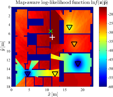
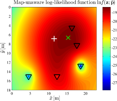
have been proposed. Estimates of all the parameters appearing in the likelihood models (12)-(15) are listed in Table I. Note that: a) the evaluation of the map-aware likelihoods (12)-(13) is more computationally demanding than that of their map-unaware counterparts (14)-(15)); b) the significant differences between map-aware and map-unaware models can be evidenced comparing a plot of (13) with that of (15) referring to the same scenario (see Fig. 7 and 8, respectively). These results show that the presence of obstructions (and, in particular, of walls) introduces jump discontinuities in the map-aware likelihood function; on the contrary, such discontinuities are not visible in the representation of its map-unaware counterpart.

Figure 7: Representation of the map-aware log-likelihood $\ln f(\mathbf{z}|\tilde{\mathbf{p}}=[\tilde{x};\tilde{y}]^{T})$ (13) evaluated for the specific map shown in Fig. 2 (the parameter values listed in Table I for RSS radios have been employed) and for the specific observation vector $\mathbf{z}$ corresponding to the measurement site #6 (identified by a white plus sign), which represents the real agent position. The 5 measurement sites selected as anchors are identified by black triangles and the peak of the log-likelihood is evidenced by a green cross (and is $1.4\,\text{m}$ away from $\mathbf{p}$).

Figure 8: Representation of the map-unaware log-likelihood $\ln f(\mathbf{z};\tilde{\mathbf{p}}=[\tilde{x};\tilde{y}]^{T})$ (15) referring to the same scenario as Fig. 7, with $\hat{\mathcal{Z}}^{\text{\tiny{NLOS}}}\equiv\mathcal{Z}^{\text{\tiny{NLOS}}}$. The 5 measurement sites selected as anchors are identified by black triangles and the peak of the log-likelihood is evidenced by a green cross (and is $2.5\,\text{m}$ away from $\mathbf{p}$).

Finally, we would like to point out that, in our opinion, a universal statistical model for RSS and TOA data is unlikely to exist and that some adjustments may be required in the models (12)-(15) if different radio devices are employed. However, we also believe that our modelling approach (starting from (6)-(9) and then involving the procedures illustrated in the Appendices) is quite general and is useful for any reader interested in modelling experimental data acquired in real world localization systems.

IV Map-Aware and Map-Unaware Localization: Algorithms and Performance

In this Section map-aware and map-unaware estimators are formulated and compared in terms of accuracy. Moreover, a brief analysis of their computational complexity is provided.

IV-A Map-Aware Estimation

The map-aware models (12) and (13) derived in paragraph III-D can be exploited to derive two types of optimal localization algorithms: the maximum a posteriori Bayesian estimator (MAPBE) and the minimum mean square error estimator (MMSEE). However, our computer simulations have evidenced that these algorithms perform similarly; for this reason in the following we focus on the MAPBE only, since its mathematical structure is simpler than that of the MMSEE. The MAPBE $\hat{\mathbf{p}}_{\text{\tiny{MAPBE}}}(\mathbf{z})$ of the agent position $\mathbf{p}$ can be evaluated as $\hat{\mathbf{p}}_{\text{\tiny{MAPBE}}}(\mathbf{z})\triangleq\arg\max_{\tilde{\mathbf{p}}}\ln f(\tilde{\mathbf{p}}|\mathbf{z})$ [38]. Exploiting (1) and the Bayes’ rule, this estimate can be expressed as

$$\hat{\mathbf{p}}_{\text{\tiny{MAPBE}}}(\mathbf{z})=\arg\max_{\tilde{\mathbf{p}}\in\mathcal{R}^{(\mathcal{Z})}}\ln f(\mathbf{z}|\tilde{\mathbf{p}})$$ (16)

where $\tilde{\mathbf{p}}$ is the trial agent position, $\mathcal{R}^{(\mathcal{Z})}$ is the search space (2) and the pdf $f(\mathbf{z}|\tilde{\mathbf{p}})$ is given by and (12) and (13) for TOA-based and RSS-based systems, respectively. The evaluation of $\hat{\mathbf{p}}_{\text{\tiny{MAPBE}}}$ requires solving a constrained LS problem since, thanks to our unified modelling, the likelihood $f(\mathbf{z}|\tilde{\mathbf{p}})$ appearing in (16) is always expressed as the product of Gaussian pdfs. However, finding the global solution to this optimization problem is not easy since its cost function is non-convex. In principle, to avoid local minima the projection onto convex sets (POCS) and the multidimensional scaling (MDS) techniques could be exploited; however, refined observation models like (12) and (13) hinder their use. It is also important to note that the cost function appearing in (16) is non-differentiable because of the discontinuous behaviour of the functions (5), (25), (26) and (27). This prevents the exact use of optimization methods based on the gradient/Hessian matrix of cost functions (e.g., steepest descent variants). For these reasons, in our computer simulations the MATLAB routine fmincon, employing sequential quadratic programming and a numerical approximation of the Hessian matrix, has been employed to solve the problem (16).

IV-B Map-Unaware Estimation

The optimal map-unaware estimator is the maximum likelihood estimator (MLE) [38]. The MLE $\hat{\mathbf{p}}_{\text{\tiny{MLE}}}(\mathbf{z})$ of $\mathbf{p}$ can be expressed as [38]

$$\hat{\mathbf{p}}_{\text{\tiny{MLE}}}(\mathbf{z})=\arg\max_{\tilde{\mathbf{p}}\in\mathcal{P}^{(\mathcal{Z})}}\ln f(\mathbf{z};\tilde{\mathbf{p}})$$ (17)

where $\tilde{\mathbf{p}}$ is the trial agent position, $\mathcal{P}^{(\mathcal{Z})}$ is the search space (3) and the pdf $f(\mathbf{z};\tilde{\mathbf{p}})$ is given by (14) and (15) for TOA-based and RSS-based systems, respectively. Note that the cost function characterising the MLE (17) is discontinuous and non-linear because of the assumption of a LOS/NLOS detection in identifying $\hat{\mathcal{Z}}^{\text{\tiny{LOS}}}$ and $\hat{\mathcal{Z}}^{\text{\tiny{NLOS}}}$. In addition, in the TOA case, the use of exponential pdfs for modelling NLOS links (see (12)) entails that $f(\mathbf{z};\tilde{\mathbf{p}})=0$ for a large portion of the domain $\mathcal{P}^{(\mathcal{Z})}$ and this complicates the search for global minima. A simple approximation that may be employed to mitigate this problem is to replace the function $\mathcal{E}\left(r;t,\mu\right)$ appearing in the right-hand side of (14) with the pdf mixture $\mathcal{M}(r;t,\mu)\triangleq 0.8\cdot\mathcal{E}\left(r;t,\mu\right)+0.2\cdot\mathcal{N}\left(r;t,\frac{\mu^{2}}{100}\right)\operatorname{u}(t-r)$, which exhibits a decreasing exponential behaviour for $r\geq t$ and a small Gaussian tail for $r<t$. Moreover, in order to further mitigate the problem of local minima, in our work the search domain $\mathcal{P}^{(\mathcal{Z})}$ has been partitioned into $N_{sub}$ sub-rectangles (whose sides have a length not exceeding $10\,\text{m}$); then, the MATLAB fmincon routine has been run $N_{sub}$ times over each of the sub-rectangles and the final MLE has been selected on the basis of a minimum-cost criterion.

IV-C Accuracy of Map-Aware and Map-Unaware Localization

Figure 9: RMSE performance of the map-aware estimator (16) and the map-unaware estimator (17), for two different values of $P_{e}^{\text{\tiny{NLOS}}}$. RSS-based localization is considered.

Figure 10: RMSE performance of the map-aware estimator (16) and the map-unaware estimator (17), for $P_{e}^{\text{\tiny{NLOS}}}=0.1$. TOA-based localization is considered.

The accuracy provided by the estimators (16) and (17) has been assessed by means of a simulation tool implementing the following procedure:

1. A measurement site, identified by the index $m_{a}$, is randomly selected in the set $\left\{1,2,...,N_{pos}\right\}$ referring to the measurement sites shown in Fig. 2 (RSS case) or in Fig. 5 (TOA case). The position of this site represents the true position $\mathbf{p}$ of the agent, so that $\mathbf{p}=\mathbf{p}_{m_{a}}$.

2. For the selected agent position, in the validation set introduced in Sec. III-D, $N_{obs}^{V}\left(m_{a}\right)$ sets of measurements associated with $N_{obs}^{V}\left(m_{a}\right)$ distinct sites are available. Each of these sites can be employed as a “virtual” anchor, and in each selected set (containing $N_{z}^{\text{\tiny{RSS}}}$ or $N_{z}^{\text{\tiny{TOA}}}$ measurements) one measurement is randomly selected and placed in the observation vector $\mathbf{z}$. To make our simulation results realistic, if $N_{obs}^{V}\left(m_{a}\right)>5$, only the observations associated with 5 random sites are chosen.

3. The estimates $\hat{\mathbf{p}}_{\text{\tiny{MAPBE}}}(\mathbf{z})$ (16) and $\hat{\mathbf{p}}_{\text{\tiny{MLE}}}(\mathbf{z})$ (17) and the associated localization errors $\left\|\mathbf{p}-\hat{\mathbf{p}}_{\text{\tiny{MAPBE}}}(\mathbf{z})\right\|$ and $\left\|\mathbf{p}-\hat{\mathbf{p}}_{\text{\tiny{MLE}}}(\mathbf{z})\right\|$ are evaluated. At the end of the simulation such errors are processed to assess the root median square error (RMSE) performance.

4. Steps 1-3 are repeated until at least $N_{runs}=2\cdot 10^{4}$ iterations have been carried out.

Some RMSE performance results $\epsilon_{\text{\tiny{MAPBE}}}$ and $\epsilon_{\text{\tiny{MLE}}}$ (referring to the MAPBE (16) and the MLE (17), respectively) are shown in Fig. 9 and 10 for RSS and TOA localization, respectively. These results evidence that:

1. In the RSS case the MAPBE always outperforms its map-unaware MLE counterpart (on the average $\epsilon_{\text{\tiny{MLE}}}^{\text{\tiny{RSS}}}=1.7\epsilon_{\text{\tiny{MAPBE}}}^{\text{\tiny{RSS}}}$ for $P_{e}^{\text{\tiny{NLOS}}}=0.1$ and $\epsilon_{\text{\tiny{MLE}}}^{\text{\tiny{RSS}}}=2.1\epsilon_{\text{\tiny{MAPBE}}}^{\text{\tiny{RSS}}}$ for $P_{e}^{\text{\tiny{NLOS}}}=0.3$; in other words, map-aware modelling enhance localization accuracy by 70% for $P_{e}^{\text{\tiny{NLOS}}}=0.1$ and by 110% for $P_{e}^{\text{\tiny{NLOS}}}=0.3$). This is due to the fact that the former technique mitigates NLOS bias (which represents a major source of error) more accurately than the latter one. In fact, maps provide a significant help whenever the bias mean predicted by (25) is significantly different from $\kappa_{b}^{\text{\tiny{RSS}}}$ (which accounts for NLOS propagation in the MLE), i.e. whenever there are several obstructions between the agent and the anchors (see Fig. 11).

2. In the TOA case map-aware and map-unaware estimators perform similarly and offer good accuracy; this is due to the fact that the TOA measurements stored in the database [25] are not affected by large NLOS biases (since all such measurements refer to close sites, often experiencing LOS conditions), so that map awareness does not play a significant role in this case. Note also that localization errors for both MAPBE and MLE are smaller than $1\,\text{m}$ for all measurement sites except #3, #8 and #12. This result can be explained referring to the specific case of site #3, for which it has been found that the large error is due to a combination of a) an anchor placement characterized by an high geometric dilution of precision [39] and b) undetected direct paths in the ranging phase (see [12]) resulting in highly biased measurements. It is also interesting to point out that the MLE is slightly more accurate than the MAPBE in the measurement sites #3, #17, #19 and #20; such results can be related to propagation effects not accounted for by our models (e.g., reflections and corridor waveguiding); however, in these cases, the difference between MLE and MAPBE RMSE is very small (few centimetres).

3. The performance gap between the RSS-based MAPBE and the MLE is large ($\epsilon_{\text{\tiny{MLE}}}^{\text{\tiny{RSS}}}-\epsilon_{\text{\tiny{MAPBE}}}^{\text{\tiny{RSS}}}=4.9\,\text{m}$ on the average), while TOA-based algorithms perform similarly ($\epsilon_{\text{\tiny{MLE}}}^{\text{\tiny{TOA}}}\simeq\epsilon_{\text{\tiny{MAPBE}}}^{\text{\tiny{TOA}}}$ on the average). This shows that maps play a significant role in improving localization accuracy when the quality of available measurements is poor, i.e., when measurements are affected by significant NLOS bias and noise (this occurs in RSS-based systems); on the contrary, if the quality is good (like in TOA UWB systems), accuracy is not significantly enhanced by map awareness (some theoretical results about this can be found in [22, 40]).

4. Map-aware fitting provides good results even if a small number of links are used in the training set (i.e., in the fitting phase); in fact, in the RSS case, only 32 links (~25% of the 116 available links) composed the training set and the performance shown in Fig. 9 have been obtained using the validation set.

Our numerical results also confirm some well-known results and, in particular, that:

1. RSS-based localization algorithms are substantially outperformed by their UWB TOA-based counterparts (on the average, $\epsilon_{\text{\tiny{MAPBE}}}^{\text{\tiny{RSS}}}=4.4\,\text{m}$ against $\epsilon_{\text{\tiny{MAPBE}}}^{\text{\tiny{TOA}}}=0.4\,\text{m}$), thanks to the superior ranging capabilities provided by UWB waveforms.

2. Significant variations in the RMSE of both TOA-based and RSS-based estimators are found when different sites are considered (similar results can be found in [36, Fig. 2], although in the scenario we consider both MAPBE and MLE perform better than the LS and MDS algorithms analysed in that reference). This is due, in the TOA case, to errors in TOA estimation originating from significant multipath [12]; in the RSS case, instead, variations originate from the spatial selectivity experienced in indoor environments.

Finally, it is worth pointing out that some additional numerical results (e.g., referring to the robustness of the proposed statistical models to parametric inaccuracies) have not been included here for space limitations, but are publicly available online (see [41]).

IV-D Complexity of Map-Aware and Map-Unaware Localization

In this Paragraph a brief analysis of the computational complexity of the MAPBE and MLE is provided. To begin, we note that the complexity associated with the evaluation of $N_{o}(\cdot,\cdot)$ is $\mathcal{O}(N_{s})$ if the shape of map obstructions can be approximated by $N_{s}$ segments, since $N_{s}$ line intersection tests are involved in such a case. Therefore, the complexity associated with the evaluation of the map-aware likelihood $f(\mathbf{z}|\tilde{\mathbf{p}})$ (see (12)-(13)) is approximately $\mathcal{O}\left(\bar{N}_{s}\cdot N_{obs}\right)$, where $\bar{N}_{s}$ is the average number of segment intersection tests accomplished in processing each of the $N_{obs}$ observations. Then, it can be inferred that the overall computational complexity of the MAPBE (16) is $\mathcal{O}\left(\bar{N}_{s}\cdot N_{obs}\cdot N_{eval}^{\text{\tiny{MAPBE}}}\right)$, where $N_{eval}^{\text{\tiny{MAPBE}}}$ denotes the overall number of times the likelihood function (12) or (13) is computed. Unluckily, the parameter $N_{eval}^{\text{\tiny{MAPBE}}}$ cannot be easily related to the other parameters of the proposed MAPBE strategy (16), since it is non-linearly related to the shape of $f(\mathbf{z}|\tilde{\mathbf{p}})$ (which is non-convex and non-differentiable) and depends strongly on the exact type of optimization method employed (see Paragraph IV-A).

As far as the map-unaware MLE (17) is concerned, its overall complexity can be expressed as $\mathcal{O}\left(N_{obs}\cdot N_{eval}^{\text{\tiny{MLE}}}\right)$ since the complexity associated with the evaluation of the likelihood $f(\mathbf{z};\tilde{\mathbf{p}})$ (14)-(15) is $\mathcal{O}\left(N_{obs}\right)$; note that $N_{eval}^{\text{\tiny{MLE}}}$ denotes the overall number of times the likelihood function (14) or (15) is evaluated and, just like $N_{eval}^{\text{\tiny{MAPBE}}}$, it cannot be easily related to the other parameters of the MLE. The constraint $\tilde{\mathbf{p}}\in\mathcal{P}^{(\mathcal{Z})}$ appearing in (17) makes even more difficult obtaining a closed expression for $N_{eval}^{\text{\tiny{MLE}}}$; however, it cannot be neglected, specially on large maps, because: a) the map-unaware likelihood functions (14)-(15) are not defined for $\tilde{\mathbf{p}}\notin\mathcal{P}^{(\mathcal{Z})}$; b) even if the likelihood domains are extended to $\mathbb{R}^{2}$, minima different from the global one are substantially less likely to be contained in the domain $\mathcal{P}^{(\mathcal{Z})}$ than in the whole $\mathbb{R}^{2}$ space. For these reasons, constrained optimization methods capable of handling the constraint $\tilde{\mathbf{p}}\in\mathcal{P}^{(\mathcal{Z})}$ must be selected (eventually employing heuristic approximations; see Paragraph IV-B).

The considerations illustrated above led us to the conclusion that an accurate estimation of the computational complexity of both (16) and (17) requires a mixed analytical/simulative approach; for more details, the reader is referred to [42], which provides an in-depth computational complexity analysis together with reduced-complexity algorithms.

V Conclusions

In this manuscript novel statistical models for map-aware indoor localization have been developed. Such models are based on experimental evidence and, in particular, rely on TOA UWB and low-frequency narrowband RSS measurements acquired in experimental campaigns. These measurements have been exploited to a) develop suitable parametric models for NLOS bias and noise, b) estimate the values of the parameters appearing in such models and c) assess the accuracy of map-aware localization techniques based on the proposed models. Our results have evidenced that map-aware localization techniques may significantly outperform their optimal map-unaware counterparts, even when state-of-the-art map-unaware algorithms based on LOS/NLOS detection and mitigation are considered. Finally, we would like to point out that:

1. The experimental campaign needed to estimate the parameters of the proposed model can be accomplished much more easily than those commonly required by fingerprinting methods.

2. The likelihoods (12) and (13) and the parameters listed in Table I can be exploited by localization algorithms operating in environments different from the ones considered here, provided that similar conditions (in terms of bandwidth of localization signals, wall thickness and composition, etc.) are experienced.

3. Even if the case of a static agent has been taken into consideration in this manuscript, the application of the developed models to navigation systems (where a mobile agent is tracked) is straightforward; for instance, (6) can be adopted as a measurement model for tracking filters (e.g., Kalman or particle filters).

Appendix A Procedures for Fitting Measurements

A-A Fitting Measurements in the Map-Aware Case

In this paragraph the two steps of the fitting procedure (see Fig. 6 and paragraph III-D) leading to the models (12) and (13) and to the parameter values listed in Table I are described.

A-A1 ML Estimation

The first step of the above mentioned procedure includes three sub-procedures: data modelling, bias estimation and noise estimation.

Data modelling - Let $(m,i)\in\mathcal{I}$ denote the link between the $m$-th and the $i$-th measurement sites, where $\mathcal{I}$ denotes the the set of the couples of indices identifying each available link. We assume that the residual rvs $\{r_{(m,i)}\triangleq z_{(m,i)}-d_{(m,i)}\}$ follow a Gaussian distribution (see the proposed data model (6))

$$f\left(\left\{r_{(m,i)}\right\}\right)=\mathcal{N}\left(r_{(m,i)};\mu_{b,i}(\mathbf{p}_{m}),\sigma_{b,i}^{2}(\mathbf{p}_{m})+\sigma_{n,i}^{2}(\mathbf{p}_{m})\right)$$ (18)

The validity of the Gaussian assumption (18) has been analysed resorting to the Anderson-Darling normality test [34, 43], which relies on the computation of a statistic, commonly denoted $A^{2*}$, and on its comparison with a fixed threshold $\gamma_{A}=1.159$ (if a significance level equal to $0.05$ is selected). We computed the $A^{2*}$ statistic for the sets of measurements $\left\{r_{(m,i)}\right\}$ referring to the RSS radios and associated with the links crossing $1$, $2$, $3$, $4$, 5, 6 walls and for these sets it was found that $A^{2*}$ is equal to $0.48$, $0.24$, $0.26$, $0.25$, $0.20$ and $0.42$, respectively; therefore, the Gaussian assumption (18) can be deemed valid in all the considered cases.

Then, the joint pdf of the experimental measurements $\left\{z_{(m,i)}\right\}$ can be put in a useful form if:

1. Statistical independence among different links is assumed.

2. The RSS bias mean $\mu_{b,i}^{\text{\tiny{RSS}}}(\mathbf{p}_{m})$ and RSS/TOA/TDOA bias variance $\sigma_{b,i}^{2}(\mathbf{p}_{m})$ are assumed to depend on the number of obstructions $t_{o,(m,i)}\triangleq N_{o}\left(\mathbf{p}_{m},\mathbf{p}_{i}\right)$ associated with the link $(m,i)$, so that $\mu_{b,i}(\mathbf{p}_{m})$ and $\sigma_{b,i}(\mathbf{p}_{m})$ can be denoted $\mu_{b}\left(t_{o,(m,i)}\right)$ and $\sigma_{b}\left(t_{o,(m,i)}\right)$, respectively. Note that $t_{o,(m,i)}$ is known at this stage.

3. The noise term $\sigma_{n,i}^{2}(\mathbf{p}_{m})$ is assumed to depend on the distance $d_{(m,i)}\triangleq d_{i}(\mathbf{p}_{m})$; such a dependence can be assessed estimating the function values $\left\{\sigma_{n,i}\right\}$ associated with $N_{d,\text{\tiny{max}}}\triangleq\max_{i}\left\lfloor d_{\text{\tiny{max}},i}/\triangle\right\rfloor$ “distance bins”; here $\triangle$ represents the distance bin size (in meters) and $d_{\text{\tiny{max}},i}$ is the maximum connectivity distance for the $i$-th anchor (see Sec. II-B). Then, a staircase approximation for each of the continuous functions $\left\{\sigma_{n,i}(\cdot)\right\}$ can be adopted; the values associated with the steps are represented by the set $\left\{\sigma_{n}\left(t\right)\right\}_{t=1}^{N_{d,\text{\tiny{max}}}}$, where $\sigma_{n}\left(t\right)$ is the noise standard deviation referring to the distance values that belong to the distance bin $[t\triangle;(t+1)\triangle]$. For this reason, $\sigma_{n,i}(\mathbf{p}_{m})$ can be denoted $\sigma_{n}\left(t_{d,(m,i)}\right)$, where $t_{d,(m,i)}$ is the index of the distance bin associated with the distance $d_{(m,i)}$ of the link $(m,i)$ and is known at this stage.

In fact, if the assumptions listed above hold, the joint pdf of $\left\{r_{(m,i)}\right\}$ (18) can be expressed as

$$\begin{split}f\left(\left\{r_{(m,i)}\right\}\right)=\prod_{(m,i)\in\mathcal{I}}\mathcal{N}&\left(r_{(m,i)};\mu_{b}\left(t_{o,(m,i)}\right),\right.\\ &\>\left.\sigma_{b}^{2}\left(t_{o,(m,i)}\right)+\sigma_{n}^{2}\left(t_{d,(m,i)}\right)\right)\end{split}$$ (19)

Bias estimation - Estimates $\left\{\hat{\mu}_{b}(t),\hat{\sigma}_{b}(t)\right\}$ of the parameters $\left\{\mu_{b}\left(t_{o,(m,i)}\right),\sigma_{b}\left(t_{o,(m,i)}\right)\right\}$ of (19) can now be evaluated. This requires processing all the measurements $\{z_{(m,i)}\}$ such that $t_{o,(m,i)}=t$, i.e., the set $\left\{r_{(m,i)}|(m,i)\in\mathcal{I}_{b}(t)\right\}$, with $\mathcal{I}_{b}(t)\triangleq\left\{(m,i)|t_{o,(m,i)}=t\right\}$, since this set represents a sufficient statistic. The MLE for $\mu_{b}\left(t_{o,(m,i)}\right)$, given the above mentioned set, is (see (19))

$$\hat{\mu}_{b}(t) \triangleq\arg\max_{\tilde{\mu}}\ln f\left(\left\{r_{(m,i)},(m,i)\in\mathcal{I}_{b}(t)\right\};\mu_{b}\left(t\right)=\tilde{\mu}\right)$$

$$=\frac{1}{\left|\mathcal{I}_{b}(t)\right|}\sum_{(m,i)\in\mathcal{I}_{b}(t)}r_{(m,i)}$$ (20)

for $t=1,...,N_{o,\text{\tiny{max}}}$, where $N_{o,\text{\tiny{max}}}$ is the maximum number of obstructions affecting the links considered in our measurement campaign; note that the right-hand side of (20) represents the sample average of the residuals $\left\{r_{(m,i)}\right\}$. Similarly, the MLE for $\sigma_{b}\left(t_{o,(m,i)}\right)$ is given by (see (19))

$$\hat{\sigma}_{b}(t)\triangleq\arg\max_{\tilde{\sigma}}\ln f\left(\left\{r_{(m,i)},(m,i)\in\mathcal{I}_{b}(t)\right\};\sigma_{b}\left(t\right)=\tilde{\sigma}\right)\\ =\arg\min_{\tilde{\sigma}}\sum_{(m,i)\in\mathcal{I}_{b}(t)}\left\{\frac{\left(r_{(m,i)}-\mu_{b}\left(t\right)\right)^{2}}{\tilde{\sigma}^{2}+\sigma_{n}^{2}\left(t_{d,(m,i)}\right)}\right.\\ \left.+2\ln\sqrt{\tilde{\sigma}^{2}+\sigma_{n}^{2}\left(t_{d,(m,i)}\right)}\vphantom{\frac{\left(r_{(m,i)}-\mu_{b}\left(t\right)\right)^{2}}{\tilde{\sigma}^{2}+\sigma_{n}^{2}\left(t_{d,(m,i)}\right)}}\right\}$$ (21)

for $t=1,...,N_{o,\text{\tiny{max}}}$. Unluckily, solving the last problem requires the knowledge of models for $\mu_{b}\left(t\right)$ and for $\sigma_{n}^{2}\left(t_{d,(m,i)}\right)$. To circumvent this, we assume that the bias mean $\mu_{b}\left(t\right)$ is well approximated by its estimate $\hat{\mu}_{b}(t)$ and that $\sigma_{n}\left(t_{d,(m,i)}\right)\ll\sigma_{b}\left(t\right)$, so that (21) can be simplified as

$$\hat{\sigma}_{b}(t) =\arg\min_{\tilde{\sigma}}\sum_{(m,i)\in\mathcal{I}_{b}(t)}\left\{\left(\frac{r_{(m,i)}-\hat{\mu}_{b}(t)}{\tilde{\sigma}}\right)^{2}+2\ln\tilde{\sigma}\right\}$$

$$=\frac{1}{\left|\mathcal{I}_{b}(t)\right|}\sum_{(m,i)\in\mathcal{I}_{b}(t)}\left(r_{(m,i)}-\hat{\mu}_{b}(t)\right)^{2}$$ (22)

The last result shows that $\hat{\sigma}_{b}(t)$ is given by a (biased) variance of the residuals $\left\{r_{(m,i)}\right\}$.

Noise estimation - The estimation of the noise standard deviation $\sigma_{n}\left(t_{d,(m,i)}\right)$ is based on the set $\left\{r_{(m,i)}|(m,i)\in\mathcal{I}_{n}(t)\right\}$ with $\mathcal{I}_{n}(t)\triangleq\left\{(m,i)|t_{d,(m,i)}=t\right\}$, since this set represents a sufficient statistic. The MLE is (see (19))

$$\hat{\sigma}_{n}(t) \triangleq\arg\max_{\tilde{\sigma}}\ln f\left(\left\{r_{(m,i)},(m,i)\in\mathcal{I}_{n}(t)\right\};\sigma_{n}\left(t\right)=\tilde{\sigma}\right)$$

$$=\arg\min_{\tilde{\sigma}}\sum_{(m,i)\in\mathcal{I}_{n}(t)}\left\{\frac{\left(r_{(m,i)}-\mu_{b}\left(t_{o,(m,i)}\right)\right)^{2}}{\sigma_{b}^{2}\left(t_{o,(m,i)}\right)+\tilde{\sigma}^{2}}\right.$$

$$\qquad\qquad\qquad\qquad\left.+2\ln\sqrt{\sigma_{b}^{2}\left(t_{o,(m,i)}\right)+\tilde{\sigma}^{2}}\vphantom{\frac{\left(r_{(m,i)}-\mu_{b}\left(t_{o,(m,i)}\right)\right)^{2}}{\sigma_{b}^{2}\left(t_{o,(m,i)}\right)+\tilde{\sigma}^{2}}}\right\}$$ (23)

for $t=1,...,N_{d,\text{\tiny{max}}}$. Like in the previous case, we assume that the bias mean $\mu_{b}\left(t_{o,(m,i)}\right)$ and variance $\sigma_{b}^{2}\left(t_{o,(m,i)}\right)$ are well approximated by their estimates $\hat{\mu}_{b}\left(t_{o,(m,i)}\right)$ and $\hat{\sigma}_{b}\left(t_{o,(m,i)}\right)$, so that (23) turns into

$$\hat{\sigma}_{n}(t)=\arg\min_{\tilde{\sigma}}\sum_{(m,i)\in\mathcal{I}_{n}(t)}\left\{\frac{\left(r_{(m,i)}-\hat{\mu}_{b}\left(t_{o,(m,i)}\right)\right)^{2}}{\hat{\sigma}_{b}^{2}\left(t_{o,(m,i)}\right)+\tilde{\sigma}^{2}}\right.\\ \left.+2\ln\sqrt{\hat{\sigma}_{b}^{2}\left(t_{o,(m,i)}\right)+\tilde{\sigma}^{2}}\vphantom{\frac{\left(r_{(m,i)}-\hat{\mu}_{b}\left(t_{o,(m,i)}\right)\right)^{2}}{\hat{\sigma}_{b}^{2}\left(t_{o,(m,i)}\right)+\tilde{\sigma}^{2}}}\right\}$$ (24)

which, unluckily, cannot be put in a closed form. For this reason, the last problem has been solved numerically resorting to the MATLAB fmincon routine.

A-A2 Evaluation of Regression Fits

In the second step of the procedure illustrated in Fig. 6, the ML estimates acquired in the first step are processed to extract two LS regression fits, one for the bias, the other one for the noise model.

Bias model fit - As already discussed in paragraph II-C, in the TOA/TDOA case a simple linear regression procedure can be employed for extracting the average parameters $t_{w}$ and $\epsilon_{r,w}$ appearing in $\mu_{b,i}(\cdot)$ (5) from the ML estimates $\left\{\hat{\mu}_{b}(t)\right\}_{t=1}^{N_{o,\text{\tiny{max}}}}$. In the RSS case, instead, the simple linear regression function, based on experimental evidence (see Fig. 11),

$$\mu_{b,i}^{\text{\tiny{RSS}}}(\mathbf{p})=\left(\mu_{b,0}^{\text{\tiny{RSS}}}+\mu_{b,m}^{\text{\tiny{RSS}}}N_{o}\left(\mathbf{p},\mathbf{p}_{i}^{a}\right)\right)\operatorname{u}_{N_{o}}$$ (25)

is proposed; here $\mu_{b,0}^{\text{\tiny{RSS}}}$ and $\mu_{b,m}^{\text{\tiny{RSS}}}$ are expressed in meters and the factor $\operatorname{u}_{N_{o}}\triangleq\operatorname{u}\left(N_{o}\left(\mathbf{p},\mathbf{p}_{i}^{a}\right)\right)$ forces $\mu_{b,i}^{\text{\tiny{RSS}}}(\mathbf{p})$ (25) to zero when $N_{o}\left(\mathbf{p},\mathbf{p}_{i}^{a}\right)=0$. Note that the selected model differs from the AF bias model, characterized by a logarithmic dependence on $N_{o}\left(\mathbf{p},\mathbf{p}_{i}^{a}\right)$.

Figure 11: Bias mean versus the number of obstructions for RSS measurements. Note that, for each ML estimate $\hat{\mu}_{b}(t)$ (20), the associated error bar is inversely proportional to the number of links $\left|\mathcal{I}_{b}(t)\right|$ available for its evaluation.

As far as the standard deviation $\sigma_{b,i}(\mathbf{p})$ of the TOA bias is concerned, the power-like model

$$\sigma_{b,i}^{\text{\tiny{TOA}}}(\mathbf{p})=\sigma_{b,0}^{\text{\tiny{TOA}}}\cdot\left(N_{o}\left(\mathbf{p},\mathbf{p}_{i}^{a}\right)\right)^{\beta_{b}^{\text{\tiny{TOA}}}}$$ (26)

is proposed; here $\beta_{b}^{\text{\tiny{TOA}}}$ is a dimensionless parameter whereas $\sigma_{b,0}^{\text{\tiny{TOA}}}$ is expressed in meters. For RSS systems, instead, our experimental results have evidenced that the bias variance is mostly constant or even decreases as the number of obstructions $N_{o}\left(\mathbf{p},\mathbf{p}_{i}^{a}\right)$ gets larger and that the linear model

$$\sigma_{b,i}^{\text{\tiny{RSS}}}(\mathbf{p})=\max\left\{\sigma_{b,0}^{\text{\tiny{RSS}}}-\sigma_{b,m}^{\text{\tiny{RSS}}}\cdot N_{o}\left(\mathbf{p},\mathbf{p}_{i}^{a}\right),0\right\}$$ (27)

can be adopted, where both the parameters $\sigma_{b,0}^{\text{\tiny{RSS}}}$ and $\sigma_{b,m}^{\text{\tiny{RSS}}}$ are expressed in meters.

Noise model fit - In various technical papers (e.g., see [8]) the additive noise term $n_{i}(\mathbf{p})$ is assumed to have the same variance for all LOS (NLOS) links, regardless of other factors, like the link distance. This noise model accounts for the inaccuracy of the algorithm adopted in extrapolating the observations $\left\{z_{i}\right\}$ in NLOS conditions, but does not account for the dependence of the performance of such an algorithm on the SNR. In this work, based on experimental evidence, we have decided to employ, for both TOA, TDOA and RSS systems, the model adopted in [13, 14, 9] and expressed by

$$\sigma_{n,i}(\mathbf{p})=\sigma_{n,0}\left(d_{i}(\mathbf{p})/d_{0}\right)^{\beta_{n}}$$ (28)

where $\sigma_{n,0}^{2}$ is the noise variance characterizing the transmitter-receiver distance $d_{0}$ and $\beta_{n}$ is the noise path loss exponent.

Finally, substituting (5), (26) and (28) (or (25), (27) and (28)) in (6) produces (12) (or (13)).

A-B Fitting Measurements in the Map-Unaware Case

A simpler procedure can be adopted for extracting regression fits in the map-unaware case. Such a procedure consists of the three steps described below.

Data modelling - On the basis of (7), each of the residuals $\left\{r_{(m,i)}\right\}$ follows a Gaussian distribution, i.e.,

$$f\left(\left\{r_{(m,i)}\right\}\right)= \prod_{i\in\mathcal{Z}^{\text{\tiny{LOS}}}}\mathcal{N}\left(r_{(m,i)};0,\sigma_{n,i}^{2}(\tilde{\mathbf{p}})\right)$$

$$\prod_{i\in\mathcal{Z}^{\text{\tiny{NLOS}}}}\mathcal{N}\left(r_{(m,i)};\kappa_{b},\sigma_{n,i}^{2}(\tilde{\mathbf{p}})+\gamma_{b}^{2}\right)$$ (29)

or a mixed Gaussian-exponential distribution (9), i.e.,

$$f\left(\left\{r_{(m,i)}\right\}\right)= \prod_{i\in\mathcal{Z}^{\text{\tiny{LOS}}}}\mathcal{N}\left(r_{(m,i)};0,\sigma_{n,i}^{2}(\tilde{\mathbf{p}})\right)$$

$$\prod_{i\in\mathcal{Z}^{\text{\tiny{NLOS}}}}\mathcal{E}\left(z_{i};0,\nu_{b}\right)$$ (30)

where $\mathcal{Z}^{\text{\tiny{LOS}}}$ and $\mathcal{Z}^{\text{\tiny{NLOS}}}$ are known in this fitting phase.

Bias model fit - On the basis of experimental data the model (29) has been adopted for modelling the RSS measurements acquired by means of a couple of radio devices operating at $169\,\text{MHz}$. The model (30), instead, has been employed to describe the TOA data collected in the Newcom++ database. The MLEs of the parameters $\kappa_{b}$ and $\gamma_{b}$ appearing in the model (29) (see Sec. II) are easily shown (using a procedure similar to that adopted in the bias model fitting for the map-aware case) to coincide with the sample average and the sample variance, respectively, of the residuals $\left\{r_{(m,i)},\forall(m,i)\in\mathcal{I}_{p}\right\}$, where $\mathcal{I}_{p}\triangleq\left\{(m,i)|t_{o,(m,i)}>0\right\}$. Similarly, if the model (30) is used, the MLE of $\nu_{b}$ coincides with the sample average of the residuals $\left\{r_{(m,i)},\forall(m,i)\in\mathcal{I}_{p}\right\}$.

Noise model fit - Following the approach adopted in the map-aware case, the noise is assumed to depend on the link distance and the ML estimate $\hat{\sigma}_{n}(t)$ of the noise standard deviation is evaluated for those links identified by a couple of indices $(m,i)$ such that $t_{d,(m,i)}=t$. Unluckily, no closed-form solution is available for this estimate, which can be expressed as (note the similarity with (24))

$$\hat{\sigma}_{n}(t)=\arg\min_{\tilde{\sigma}}\sum_{(m,i)\in\mathcal{I}_{n}(t)}\left\{\frac{\left(r{}_{(m,i)}-\mu_{b,(m,i)}\right)^{2}}{\sigma_{b,(m,i)}^{2}+\tilde{\sigma}^{2}}\right.\\ \left.+2\ln\sqrt{\sigma_{b,(m,i)}^{2}+\tilde{\sigma}^{2}}\vphantom{\frac{\left(r{}_{(m,i)}-\mu_{b,(m,i)}\right)^{2}}{\sigma_{b,(m,i)}^{2}+\tilde{\sigma}^{2}}}\right\}$$ (31)

for $t=1,...,N_{d,\text{\tiny{max}}}$. It is also important to mention that $\mu_{b,(m,i)}$ and $\sigma_{b,(m,i)}$ are defined as: a) $\mu_{b,(m,i)}\triangleq\kappa_{b}$ and $\sigma_{b,(m,i)}\triangleq\gamma_{b}$, respectively, if the NLOS bias is modelled as a Gaussian rv (see (7) and (29)); b) $\mu_{b,(m,i)}\triangleq\nu_{b}$ and $\sigma_{b,(m,i)}\triangleq\nu_{b}^{2}$, respectively, if the NLOS bias is modelled as an exponential random variable (see (9) and (30)). In both cases we have found that the quantities $\left\{\hat{\sigma}_{n}(t)\right\}$ do exhibit a monotonic dependence on the distance (due to all propagation mechanisms not accounted for by a map-unaware model); despite this, the model (28) has been selected as a regression function for $\sigma_{n,i}(\mathbf{p})$.

Finally, substituting (28) in (7) produces the likelihood function (15) proposed for map-unaware RSS systems. Similarly, substituting (28) in (9) yields the likelihood function (14) referring to map-unaware TOA systems.

Francesco Montorsi (S’06) received both the Laurea degree (cum laude) and the Laurea Specialistica degree (cum laude) in Electronic Engineering from the University of Modena and Reggio Emilia, Italy, in 2007 and 2009, respectively. He received the Ph.D degree in Information and Communications Technologies (ICT) from the University of Modena and Reggio Emilia in 2013. He is employed as embedded system engineer for an ICT company since 2013. In 2011 he was a visiting PhD student at the Wireless Communications and Network Science Laboratory of Massachusetts Institute of Technology (MIT). His research interests are in the area of localization and navigation systems, with emphasis on statistical signal processing (linear and non-linear filtering, detection and estimation problems), model-based design and model-based performance assessment. Dr. Montorsi is a member of IEEE Communications Society and served as a reviewer for the IEEE Transactions on Wireless Communications,IEEE Transactions on Signal Processing, IEEE Wireless Communications Letters and several IEEE conferences. He received the GTTI Award for PhD Theses in the field of Communication Technologies in 2013 from the Italian Telecommunications and Information Theory Group (GTTI).

Fabrizio Pancaldi was born in Modena, Italy, in July 1978. He received the Dr. Eng. Degree in Electronic Engineering (cum laude) and the Ph. D. degree in 2006, both from the University of Modena and Reggio Emilia, Italy. From March 2006 he is holding the position of Assistant Professor at the same university and he gives the courses of Telecommunication Networks and ICT Systems. He works in the field of digital communications, both radio and powerline. His particular interests lie in the wide area of digital communications, with emphasis on channel equalization, statistical channel modelling, space-time coding, radio localization, channel estimation and clock synchronization.

Giorgio M. Vitetta (S’89-M’91-SM’99) was born in Reggio Calabria, Italy, in April 1966. He received the Dr. Ing. degree in electronic engineering (cum laude) in 1990, and the Ph.D. degree in 1994, both from the University of Pisa, Pisa, Italy. From 1995 to 1998, he was a Research Fellow with the Department of Information Engineering, University of Pisa. From 1998 to 2001, he was an Associate Professor with the University of Modena and Reggio Emilia, Modena, Italy, where he is currently a full Professor. His main research interests lie in the broad area of communication theory, with particular emphasis on detection/equalization/synchronization algorithms for wireless communications, statistical modelling of wireless and powerline channels, ultrawideband communication techniques and applications of game theory to wireless communications. Dr. Vitetta is serving as an Editor of the IEEE Wireless Communications Letters and as an Area Editor of the IEEE Transactions on Communications.

References

- [1] N. Patwari, J. Ash, S. Kyperountas, A. O. Hero, III, R. Moses, and N. Correal, “Locating the nodes: cooperative localization in wireless sensor networks,” IEEE Signal Processing Mag., vol. 22, no. 4, pp. 54–69, Jul. 2005.
- [2] K. Pahlavan and J. Makela, “Indoor geolocation science and technology,” IEEE Commun. Mag., vol. 40, no. 2, pp. 112–118, Feb. 2002.
- [3] E. Falletti and M. Luise, Eds., Deliverable Number: DB.1, Review of Satellite, Terrestrial Outdoor, and Terrestrial Indoor Positioning Techniques. NEWCOM++, 2009.
- [4] D. Dardari, A. Conti, J. Lien, and M. Z. Win, “The Effect of Cooperation on Localization Systems Using UWB Experimental Data,” EURASIP J. on Advances in Signal Processing, pp. 1–12, 2008.
- [5] T. S. Rappaport, Wireless Communications: Principles and Practice. Prentice-Hall, 2002.
- [6] M. Lott and I. Forkel, “A Multi-Wall-and-Floor Model for Indoor Radio Propagation,” in IEEE Veh. Tech. Conf., Rhodes, 2001, pp. 464–468.
- [7] X. Li, “Collaborative Localization With Received-Signal Strength in Wireless Sensor Networks,” IEEE Trans. Veh. Technol., vol. 56, no. 6, pp. 3807–3817, Nov. 2007.
- [8] K. Yu and Y. J. Guo, “Statistical NLOS Identification Based on AOA, TOA, and Signal Strength,” IEEE Trans. Veh. Technol., vol. 58, no. 1, pp. 274–286, Jan. 2009.
- [9] S. Venkatesh and R. M. Buehrer, “Non-line-of-sight identification in ultra-wideband systems based on received signal statistics,” IET Microw. Antennas Propag., vol. 1, no. 6, pp. 1120 –1130, Dec. 2007.
- [10] S. Mazuelas, A. Bahillo, R. M. Lorenzo, P. Fernandez, F. A. Lago, E. Garcia, J. Blas, and E. J. Abril, “Robust Indoor Positioning Provided by Real-Time RSSI Values in Unmodified WLAN Networks,” IEEE J. of Sel. Topics in Signal Process., vol. 3, no. 5, pp. 821–831, Oct. 2009.
- [11] J. Yang and Y. Chen, “Indoor Localization Using Improved RSS-Based Lateration Methods,” in IEEE Global Telecommun. Conf., Hawaii, 2009, pp. 1–6.
- [12] B. Alavi and K. Pahlavan, “Modeling of the TOA-based Distance Measurement Error Using UWB Indoor Radio Measurements,” IEEE Commun. Letters, vol. 10, no. 4, pp. 275–277, Apr. 2006.
- [13] S. Venkatesh and R. M. Buehrer, “NLOS Mitigation Using Linear Programming in Ultrawideband Location-Aware Networks,” IEEE Trans. Veh. Technol., vol. 56, no. 5, pp. 3182–3198, Sep. 2007.
- [14] D. B. Jourdan, D. Dardari, and M. Z. Win, “Position Error Bound for UWB Localization in Dense Cluttered Environments,” in IEEE Int. Conf. on Communications, Istanbul, 2006, pp. 3705–3710.
- [15] F. Montorsi, F. Pancaldi, and G. M. Vitetta, “Statistical Characterization and Mitigation of NLOS Bias in UWB Localization Systems,” Advances in Electronics and Telecommunications, vol. 2, no. 4, pp. 11–17, Dec. 2011.
- [16] F. Montorsi, “Localization and Tracking for Indoor Environments,” Ph.D. dissertation, University of Modena and Reggio Emilia, 2013.
- [17] S.-H. Fang, T.-N. Lin, and K.-C. Lee, “A Novel Algorithm for Multipath Fingerprinting in Indoor WLAN Environments,” IEEE Trans. Wireless Commun., vol. 7, no. 9, pp. 3579–3588, Sep. 2008.
- [18] C. Figuera, I. Mora-Jimenez, A. Guerrero-Curieses, J. L. Rojo-Alvarez, E. Everss, M. Wilby, and J. Ramos-Lopez, “Nonparametric Model Comparison and Uncertainty Evaluation for Signal Strength Indoor Location,” IEEE Trans. On Mobile Computing, vol. 8, no. 9, pp. 1250–1264, Sep. 2009.
- [19] M. Bshara, U. Orguner, F. Gustafsson, and L. V. Biesen, “Fingerprinting Localization in Wireless Networks Based on Received-Signal-Strength Measurements: A Case Study on WiMAX Networks,” IEEE Trans. Veh. Technol., vol. 59, no. 1, pp. 283–294, Jan. 2010.
- [20] H. Wang, “Bayesian Radio Map Learning for Robust Indoor Positioning,” in Int. Conf. on Indoor Positioning and Indoor Navigation, Guimaraes, 2011, pp. 1–6.
- [21] H. Liu, H. Darabi, P. Banerjee, and J. Liu, “Survey of Wireless Indoor Positioning Techniques and Systems,” IEEE Trans. on Syst., Man Cybern., vol. 37, no. 6, pp. 1067–1080, Nov. 2007.
- [22] F. Montorsi, S. Mazuelas, G. M. Vitetta, and M. Z. Win, “On the Performance Limits of Map-Aware Localization,” IEEE Transactions on Information Theory, vol. 59, no. 8, pp. 5023–5038, Aug. 2013.
- [23] I. Guvenc and C.-C. Chong, “A Survey on TOA Based Wireless Localization and NLOS Mitigation Techniques,” IEEE Commun. Surveys & Tutorials, vol. 11, no. 3, pp. 107–124, 2009.
- [24] “Embit EMB-WMB169T radio datasheet,” Available online at http://www.embit.eu.
- [25] “WPR.B database,” Available online at http://www.vicewicom.eu and at http://frm.users.sourceforge.net/publications.html.
- [26] P. Vandewalle, J. Kovacevic, and M. Vetterli, “Reproducible research in signal processing - what, why, and how,” IEEE Signal Processing Mag., vol. 26, no. 3, pp. 37–47, May 2009.
- [27] C. Alippi, A. Mottarella, and G. Vanini, “A RF map-based localization algorithm for indoor environments,” in IEEE Int. Symp. on Circuits and Systems, Kobe, 2005, pp. 652–655.
- [28] D. Porrat and D. Cox, “UHF Propagation in Indoor Hallways,” IEEE Trans. Wireless Commun., vol. 3, no. 4, pp. 1188–1198, Jul. 2004.
- [29] R. J. C. Bultitude, “Measurement, Characterization and Modeling of Indoor 800/900 MHz Radio Channels for Digital Communications,” IEEE Commun. Mag., vol. 25, no. 6, pp. 5–12, Jun. 1987.
- [30] J. Leung, “Hybrid Waveguide Theory-Based Modeling of Indoor Wireless Propagation,” Master’s thesis, University of Toronto, 2009.
- [31] D. Söderman, “A 2D Indoor Propagation Model Based on Waveguiding, Mode Matching and Cascade Coupling,” Master’s thesis, KTH - School of Electrical Engineering, 2012.
- [32] M. S. Reynolds, N. A. Gershenfeld, and A. Lippman, “Low Frequency Indoor Radiolocation,” Ph.D. dissertation, Massachusetts Institute of Technology, 2003.
- [33] B. Radunovic, D. Gunawardena, P. Key, A. Proutiere, N. Singh, V. Balan, and G. Dejean, “Rethinking Indoor Wireless: Low Power, Low Frequency, Full-duplex,” Microsoft Corporation, Tech. Rep., 2009.
- [34] P. Closas, J. Arribas, and C. Fern, “Testing for normality of UWB-based distance measurements by the Anderson-Darling statistic,” in Future Network and Mobile Summit Conf. Proc., Florence, 2010, pp. 1–8.
- [35] D. Dardari and A. A. D. Amico, “LOS / NLOS Detection for UWB Signals : A Comparative Study Using Experimental Data,” in IEEE Int. Symp. on Wireless Pervasive Computing, Modena, 2010, pp. 169–173.
- [36] M. R. Gholami, E. G. Strom, F. Sottile, D. Dardari, A. Conti, S. Gezici, M. Rydstrom, and M. A. Spirito, “Static Positioning Using UWB Range Measurements,” in Future Network and Mobile Summit Conf. Proc., Florence, 2010, pp. 1–10.
- [37] C. M. Bishop, Pattern Recognition and Machine Learning. Springer, 2006.
- [38] S. Kay, Fundamentals of Statistical Signal Processing: Estimation Theory. Prentice Hall, 1993, vol. I.
- [39] I. Sharp, K. Yu, and Y. J. Guo, “GDOP Analysis for Positioning System Design,” IEEE Trans. Veh. Technol., vol. 58, no. 7, pp. 3371–3382, 2009.
- [40] F. Montorsi, S. Mazuelas, F. Pancaldi, G. M. Vitetta, and M. Z. Win, “On the Impact of A Priori Information on Localization Accuracy and Complexity,” in IEEE Int. Conf. on Commun., Budapest, 2013, pp. 5792–5797.
- [41] F. Montorsi, F. Pancaldi, and G. M. Vitetta, “Map-Aware RSS Localization Models and Algorithms Based on Experimental Data,” in IEEE Int. Conf. on Commun., Budapest, 2013, pp. 5798–5803.
- [42] ——, “Reduced-Complexity Algorithms for Indoor Map-Aware Localization Systems,” Submitted to IEEE Trans. Wireless Commun., 2014.
- [43] T. W. Anderson, “Asymptotic theory of certain goodness-of-fit criteria based on stochastic processes,” Ann. Math. Stat., vol. 23, Jun. 1952.
![[Uncaptioned image]](/html/1402.3783/assets/Montorsi.jpg) |