Spectral viscosity method with generalized Hermite functions for nonlinear conservation laws

Abstract

In this paper, we propose new spectral viscosity methods based on the generalized Hermite functions for the solution of nonlinear scalar conservation laws in the whole line. It is shown rigorously that these schemes converge to the unique entropy solution by using compensated compactness arguments, under some conditions. The numerical experiments of the inviscid Burger’s equation support our result, and it verifies the reasonableness of the conditions.

1 Introduction

The spectral methods [9] approximate the exact solution of partial differential equations by seeking an “good” projection in the linear subspace spanned by various orthogonal systems of special functions. The resulting spectral accuracy is highly preferred than any other numerical method, especially when the solution is known to be globally smooth enough. Therefore, they are very appropriate for the elliptic and parabolic equations, thanks to the regularization properties of the operators. When mentioning the nonlinear conservation laws, it is well known that the solution may develop spontaneous jump discontinuity, i.e., shock waves. This irregularity of the solution destroys not only the accuracy of the spectral approximations at the point of discontinuity, but also that in the entire computational domain. It causes the oscillations throughout the domain, which is the so-called Gibb’s phenomenon. Moreover, the instability is induced in the nonlinear case. It is shown in [25] that the usual spectral approximate solution may not converge to the entropy solution, the physically relevant one.

Despite all these deficiencies, many mathematicians still pay their efforts to deal with these issues. The problems caused by the irregularity have already been solved for piecewise smooth functions in bounded domain or periodic piecewise smooth function in unbounded domain by filter techniques or reconstruction methods such as the Gegenbauer partial sum, see details in a series of papers [12], [11], [10], [28] and references therein. And the instability of the usual spectral approximations can be avoided by introducing the vanishing viscosity, which was first established by E. Tadmor [24]. The main idea of the spectral viscosity method is the use of artificial diffusion to stabilize the spectral computation without sacrificing its spectral accuracy. The periodic spectral viscosity method has been further investigated in [19], [25] and [20], etc. The nonperiodic Legendre spectral viscosity method is first introduced by Y. Maday, et. al. [18]. H. Ma proposed the nonperiodic Chebyshev-Legendre spectral viscosity method in [16], [17]. For more literatures related to the spectral viscosity methods with various orthogonal basis in bounded domain, we refer the readers to [6], [8], [13] and references therein.

As we know, a large amount of physical problems are modeled in unbounded domain. During the past two decades, more attentions were attracted to the numerical solutions of differential equations in unbounded domains. Among the existing literature, the Hermite and Laguerre spectral methods are the most commonly used approaches based on orthogonal polynomials in infinite interval, referring to [7], [29]. Although the Hermite polynomials appear to be a natural choice of orthogonal basis of $L^{2}(\mathbb{R})$, it is not as popular as Fourier series and Chebyshev polynomials, due to its poor resolution (see [9]) and the lack of the analogue of fast Fourier transformation (FFT), see [4]. However, it is shown in [2] that the poor resolution can be remedied by a suitable choice of scaling factor. Some further investigations on the scaling factor can be found in [26] and Chapter 7, [22]. Recently, a practical guideline of choosing the suitable scaling factors for Gaussian/super-Gaussian functions is summarized by S. S.-T. Yau and the author in [14], where the Hermite spectral method is used to resolve the posterior conditional density function of the states in nonlinear filtering problems.

The literatures on the spectral method in unbounded domains have already been not as rich as those in bounded domains, let alone the spectral viscosity method in unbounded domains. As far as we know, J. Aguirre and J. Rivas [1] is the only paper that considered the spectral viscosity method based on the Hermite functions. However, they defined the Hermite functions in the weighted $L_{w}^{2}(\mathbb{R})$, where $w(x)={e^{x^{2}}}$. No scaling factor is introduced there. This essentially causes their involved theoretical proof of the convergence rate of their proposed scheme. Also it is more costly when they try to implement their scheme numerically.

In this paper, we shall revisit the nonlinear scalar conservation laws in $\mathbb{R}$:

$$\left\{\begin{aligned} \frac{\partial u}{\partial t}+\frac{\partial f(u)}{\partial x}=&0,\quad x\in\mathbb{R},\,t>0\\ u(x,0)=&u_{0}(x),\quad x\in\mathbb{R},\end{aligned}\right.$$ (1.1)

where $f\in C^{1}$ is a smooth nonlinear function and $u_{0}\in L^{\infty}(\mathbb{R})$. In general, the spontaneous jump discontinuity may be developed. Therefore, we can not expect the classical solutions to this problem. Moreover, we restrict ourselves to the physically relevant weak solution, the entropy solution, by imposing the entropy condition

$$\frac{\partial U(u)}{\partial t}+\frac{\partial F(u)}{\partial x}\leq 0$$ (1.2)

in the sense of distributions, for all entropy pairs $(U,F)$, with $U\in C^{2}$ convex and $F^{\prime}(u)=U^{\prime}(u)f^{\prime}(u)$, see [21].

We propose Hermite spectral viscosity methods based on generalized Hermite functions with two different viscosity terms.

1. with viscosity term $\epsilon\partial_{x}\mathcal{D}_{x}u$: The approximate solution $u_{N}$ is obtained by solving

   $$\left\{\begin{aligned} \partial_{t}u_{N}+\partial_{x}(P_{N+1}f(u_{N}))-\epsilon_{N}\partial_{x}\mathcal{D}_{x}Q_{m_{N}}u_{N}=&0,\quad x\in\mathbb{R},\,t\in(0,T),\\ u_{N}(x,0)=&P_{N}u_{0}(x),\quad x\in\mathbb{R},\end{aligned}\right.$$ (1.3)

   where $P_{N+1}$ is an $L^{2}$-orthogonal projection operator defined in (2.15), $\epsilon_{N}\rightarrow 0$ is a positive parameter as $N$ tends to $\infty$, and $Q_{m_{N}}$ is a viscosity operator which modifies only the high modes of the Fourier-Hermite expansion. That is,

   $$Q_{m_{N}}\left(\sum_{k=0}^{N}\hat{\phi}_{k}(t)H_{k}^{\alpha}(x)\right)=\sum_{k=0}^{N}\hat{q}_{k}\hat{\phi}_{k}(t)H_{k}^{\alpha}(x),$$ (1.4)

   with

   $$\left\{\begin{aligned} \hat{q}_{k}=0,\quad&\textup{if}\quad k\leq m_{N}\\ 1-\frac{m_{N}}{k}\leq\hat{q}_{k}<1,\quad&\textup{if}\quad k>m_{N}\end{aligned}\right.,$$ (1.5)

   and $m_{N}<N$ is a positive integer tending to $\infty$ as $N$ tends to $\infty$, where $H_{k}^{\alpha}(x)$ are the generalized Hermite functions defined in (2.2).

2. with viscosity term $\epsilon\mathcal{L}_{\alpha}u$: The approximate solution $v_{N}$ is obtained by solving

   $$\left\{\begin{aligned} \partial_{t}v_{N}+\partial_{x}(P_{N+1}f(v_{N}))+\epsilon_{N}\mathcal{L}_{\alpha}v_{N}=&0,\quad x\in\mathbb{R},\,t\in(0,T),\\ v_{N}(x,0)=&P_{N}u_{0}(x),\quad x\in\mathbb{R},\end{aligned}\right.$$ (1.6)

   where $P_{N+1}$, $\epsilon_{N}$ are the same as those in (I), and $\mathcal{L}_{\alpha}$ is defined in (2.4).

Nevertheless, compared to the scheme in [1], the schemes in our paper have at least two advantages:

• Our scheme (II) is numerically stable, due to its symmetry and positivity, while the stability of the scheme in [1] and our scheme (I) can not be guaranteed;

• Our schemes can be implemented efficiently with the help of the scaling factor. The better resolution and fewer oscillations are retained with much smaller truncation terms $N$ even without viscosity.

In this paper, we shall develop two efficient schemes to solve the nonlinear conservation laws in $\mathbb{R}$. The convergences of the schemes have been shown under some reasonable condtions (3.9) or (3.36). It is hard to tell whether these conditions are weaker or stronger than the one in [1], i.e., $||xu_{N}||_{\infty}<C$, independent of $N$, due to the unbounded domain $\mathbb{R}\times(0,T)$.

The paper is organized as follows. In section 2, we give the definition of the generalized Hermite functions and their properties. The new Hermite spectral viscosity methods are proposed and their convergences have been rigorously shown in section 3. In section 4, the inviscid Burger’s equation has been numerically solved by our schemes. The reasonableness of the conditions in the convergence theorems have been verified numerically.

2 Generalized Hermite functions

In this section, we introduce the generalized Hermite functions and derive their properties inherited from the Hermite polynomials.

Let $L^{2}(\mathbb{R})$ be the Lebesgue space, equipped with the norm $||\cdot||=(\int_{\mathbb{R}}|\cdot|^{2}dx)^{\frac{1}{2}}$ and the scalar product $\langle\cdot,\cdot\rangle$. Moreover, we shall denote $||\circ||_{\infty}=||\circ||_{L^{\infty}(\mathbb{R}\times(0,T))}=\sup_{\mathbb{R}\times[0,T]}|\circ|$ and $||\circ||^{2}_{L^{2}(0,T;L^{2}(\mathbb{R}))}:=\int_{0}^{T}||\circ||^{2}dt$.

In the sequel, we shall follow the conventional notations in the asymptotic analysis: $a\sim b$ means that there exist some generic constants $C_{1},C_{2}>0$ such that $C_{1}a\leq b\leq C_{2}a$; $a\lesssim b$ means that there exists some generic constant $C_{3}>0$ such that $a\leq C_{3}b$.

Let $\mathcal{H}_{n}(x)$ be the physical Hermite polynomials, i.e., $\mathcal{H}_{n}(x)=(-1)^{n}e^{x^{2}}\partial_{x}^{n}e^{-x^{2}}$, $n\geq 0$. The three-term recurrence

$$\mathcal{H}_{0}\equiv 1,\quad\mathcal{H}_{1}(x)=2x\quad\textup{and}\quad\mathcal{H}_{n+1}(x)=2x\mathcal{H}_{n}(x)-2n\mathcal{H}_{n-1}(x).$$ (2.1)

is handy in implementation. One of the well-known and useful fact of Hermite polynomials is that they are mutually orthogonal with respect to the weight $w(x)=e^{-x^{2}}$. We define the generalized Hermite functions with the scaling factor $\alpha>0$ as

$$H_{n}^{\alpha}(x)=\left(\frac{\alpha}{2^{n}n!\sqrt{\pi}}\right)^{\frac{1}{2}}\mathcal{H}_{n}(\alpha x)e^{-\frac{1}{2}\alpha^{2}x^{2}},$$ (2.2)

for $n\geq 0$. It is readily to derive the following properties for the generalized Hermite functions (2.2):

1. The $\{H_{n}^{\alpha}(x)\}_{n\in\mathbb{Z^{+}}}$ forms an orthonormal basis of $L^{2}(\mathbb{R})$, i.e.

   $$\int_{\mathbb{R}}H_{n}^{\alpha}(x)H_{m}^{\alpha}(x)dx=\delta_{nm},$$ (2.3)

   where $\delta_{nm}$ is the Kronecker function.

2. $H_{n}^{\alpha}(x)$ is the $n$th eigenfunction of the following Strum-Liouville problem

   $$\mathcal{L}_{\alpha}u(x):=-e^{\frac{1}{2}\alpha^{2}x^{2}}\frac{d}{dx}\left(e^{-\alpha^{2}x^{2}}\frac{d}{dx}\left(e^{\frac{1}{2}\alpha^{2}x^{2}}u(x)\right)\right)=\lambda_{n}u(x),$$ (2.4)

   with the corresponding eigenvalue

   $$\lambda_{n}=2\alpha^{2}n.$$ (2.5)

3. By convention, $H_{n}^{\alpha}\equiv 0$, for $n<0$. For $n\geq 0$, the three-term recurrence is inherited from the Hermite polynomials:

   $$xH_{n}^{\alpha}(x)= \frac{\sqrt{\lambda_{n+1}}}{2\alpha^{2}}H_{n+1}^{\alpha}(x)+\frac{\sqrt{\lambda_{n}}}{2\alpha^{2}}H_{n-1}^{\alpha}(x).$$ (2.6)

4. The derivative of $H_{n}^{\alpha}(x)$ with respect to $x$ gives

   $${\frac{d}{dx}}H_{n}^{\alpha}(x)= -\frac{\sqrt{\lambda_{n+1}}}{2}H_{n+1}^{\alpha}(x)+\frac{\sqrt{\lambda_{n}}}{2}H_{n-1}^{\alpha}(x).$$ (2.7)

   For convenience, let $\mathcal{D}_{x}={\frac{d}{dx}}+\alpha^{2}x$. Then

   $$\mathcal{D}_{x}H_{n}^{\alpha}(x)=\sqrt{2\alpha^{2}n}H_{n-1}^{\alpha}(x)=\sqrt{\lambda_{n}}H_{n-1}^{\alpha}(x).$$ (2.8)

5. The “orthogonality” of $\{\mathcal{D}_{x}H_{n}^{\alpha}(x)\}_{n\in\mathbb{Z}^{+}}$ follows immediately from (2.3), i.e.,

   $$\int_{\mathbb{R}}\mathcal{D}_{x}H_{n}^{\alpha}(x)\mathcal{D}_{x}H_{m}^{\alpha}(x)dx=2\alpha^{2}n\delta_{nm}=\lambda_{n}\delta_{nm}{.}$$ (2.9)

Any function $u(x)\in L^{2}(\mathbb{R})$ can be written in the form

$$u(x)=\sum_{n=0}^{\infty}\hat{u}_{n}H_{n}^{\alpha}(x),$$ (2.10)

with

$$\hat{u}_{n}=\int_{\mathbb{R}}u(x)H_{n}^{\alpha}(x)dx{,}$$ (2.11)

where $\{\hat{u}_{n}\}_{n=0}^{\infty}$ are the Fourier-Hermite coefficients.

Let us denote the linear subspace of $L^{2}(\mathbb{R})$ spanned by the first $N$ generalized Hermite functions by

$$\mathcal{R}_{N}:=\textup{span}\{H_{0}^{\alpha}(x),\cdots,H_{N}^{\alpha}(x)\}.$$ (2.12)

Remark 2.1

Actually, we have the norms $||{\frac{d}{dx}}\phi||$ controlled by $||\mathcal{D}_{x}\phi||$ and $||\phi||$, for any $\phi\in\mathcal{R}_{N}$. Let us consider

$$\left|\left|\frac{d}{dx}\phi\right|\right|^{2}= \left|\left|\sum_{k=0}^{N}\hat{\phi}_{k}\left(-\frac{\sqrt{\lambda_{k+1}}}{2}H_{k+1}^{\alpha}+\frac{\sqrt{\lambda_{k}}}{2}H_{k-1}^{\alpha}\right)\right|\right|^{2}$$

$$= \sum_{k,l=0}^{N}\hat{\phi}_{k}\hat{\phi}_{l}\int_{\mathbb{R}}\left(\frac{\sqrt{\lambda_{k+1}}}{2}H_{k+1}^{\alpha}+\frac{\sqrt{\lambda_{k}}}{2}H_{k-1}^{\alpha}\right)\left(-\frac{\sqrt{\lambda_{l+1}}}{2}H_{l+1}^{\alpha}+\frac{\sqrt{\lambda_{l}}}{2}H_{l-1}^{\alpha}\right)dx$$

$$\overset{\eqref{orthogonal}}{=} \frac{1}{4}\sum_{k=0}^{N}\hat{\phi}_{k}^{2}(\lambda_{k+1}+\lambda_{k})-\frac{1}{4}\sum_{k=0}^{N-2}\hat{\phi}_{k+2}\hat{\phi}_{k}\sqrt{\lambda_{k+2}\lambda_{k+1}}-\frac{1}{4}\sum_{k=2}^{N}\hat{\phi}_{k}\hat{\phi}_{k-2}\sqrt{\lambda_{k}\lambda_{k-1}}$$

$$\leq \frac{1}{2}\sum_{k=0}^{N}\hat{\phi}_{k}^{2}\lambda_{k+1}+\frac{1}{2}\sum_{k=0}^{N}\hat{\phi}_{k}^{2}\lambda_{k}\overset{\eqref{eqn-lambda}}{=}\sum_{k=0}^{N}\hat{\phi}_{k}^{2}\lambda_{k}+\alpha^{2}\sum_{k=0}^{N}\hat{\phi}_{k}^{2}=||\mathcal{D}_{x}\phi||^{2}+\alpha^{2}||\phi||^{2},$$ (2.13)

where the inequality follows from the fact that

$$\left|\hat{\phi}_{k+2}\hat{\phi}_{k}\sqrt{\lambda_{k+2}\lambda_{k+1}}\right|\leq \frac{1}{2}\left(\hat{\phi}_{k+2}^{2}\lambda_{k+2}+\hat{\phi}_{k}^{2}\lambda_{k+1}\right),$$

for $k=0,\cdots,N-2$. Similarly, we can get

$$||x\phi||^{2}\lesssim\frac{1}{\alpha^{4}}\left[||\mathcal{D}_{x}\phi||^{2}+\alpha^{2}||\phi||^{2}\right].$$ (2.14)

We define the $L^{2}$-orthogonal projection $P_{N}^{\alpha}:\,L^{2}(\mathbb{R})\rightarrow\mathcal{R}_{N}$: given $v\in L^{2}(\mathbb{R})$, we have

$$\langle v-P_{N}^{\alpha}v,\phi\rangle=0,$$ (2.15)

for all $\phi\in\mathcal{R}_{N}$. More precisely, it can be written as

$$P_{N}^{\alpha}v(x)=\sum_{n=0}^{N}\hat{v}_{n}H_{n}^{\alpha}(x),$$

where $\hat{v}_{n}$, $n=0,\ldots,N$, are the Fourier-Hermite coefficients defined in (2.11).

To establish the convergence rate of the Hermite spectral method, we shall also state the convergence rate of the orthogonal approximation. The error estimate of the orthogonal projection onto $\mathcal{R}_{N}$ is readily shown in Theorem 4.2, [23] for $\alpha=1$ and it can be trivially extended for $\alpha>0$.

Lemma 2.1

For any $\mathcal{D}_{x}^{m}u\in L^{2}(\mathbb{R})$ with $m\geq 0$,

$$||\mathcal{D}_{x}^{l}(u-P_{N}^{\alpha}u)||\lesssim\alpha^{l-m}N^{\frac{l-m}{2}}||\mathcal{D}_{x}^{m}u||,\quad 0\leq l\leq m.$$

In the sequel, the superscript $\alpha$ in $P_{N}^{\alpha}$ will be dropped if no confusion will arise.

3 The Hermite spectral viscosity method

It is well known that the entropy solution to (1.1) can be obtained as the limit when the artificially introduced viscosity term vanishes. In this section, we shall introduce two appropriate viscosity terms $\epsilon\partial_{x}\mathcal{D}_{x}u$ and $\epsilon\mathcal{L}_{\alpha}u$. The convergences of both schemes will be shown under the assumption that the approximate solutions are uniformly bounded in $L^{\infty}$ norm. It is well known that the numerical solution is bounded in a finite interval, but not that in unbounded domain. This interesting question will not be discussed in this paper.

With the viscosity term $\epsilon\partial_{x}\mathcal{D}_{x}u$, the viscosity operator $Q_{m_{N}}$ has been introduced in the spectral scheme as in [1], where only the high frequency terms appear in the artificial viscosity. The convergence of this scheme has been shown under the condition (3.9). The reasonableness of this condition in the inviscid Burger’s equation has been verified in Table 4.1.

3.1 With viscosity term $\epsilon\partial_{x}\mathcal{D}_{x}u$

Let us discuss the viscosity operator $Q_{m_{N}}$ first.

Lemma 3.2

Let $Q_{m_{N}}$ be defined as in (1.4) and (1.5). Then

$$||\mathcal{D}_{x}\phi||^{2}\lesssim||\mathcal{D}_{x}Q_{m_{N}}\phi||^{2}+\alpha^{2}m_{N}^{2}||\phi||^{2},$$ (3.1)

and

$$||\mathcal{D}_{x}Q_{m_{N}}\phi||^{2}\lesssim||\mathcal{D}_{x}\phi||^{2}+\alpha^{2}m_{N}^{2}||\phi||^{2}{,}$$ (3.2)

for all $\phi\in\mathcal{R}_{N}$.

Proof. Let us show (3.1) in detail only, and (3.2) can be obtained by the similar argument. Let $\phi=\sum_{k=0}^{N}\hat{\phi}_{k}H_{k}^{\alpha}(x)$ and $R_{m_{N}}=I-Q_{m_{N}}$, where $I$ is the identity operator, then

$$||\mathcal{D}_{x}\phi||^{2}\lesssim||\mathcal{D}_{x}Q_{m_{N}}\phi||^{2}+||\mathcal{D}_{x}R_{m_{N}}\phi||^{2}.$$ (3.3)

We split $\phi$ in dyadic parts $\phi(x)=\sum_{k=0}^{m_{N}}\hat{\phi}_{k}H_{k}^{\alpha}(x)+\sum_{j=1}^{J}\phi^{j}(x)$, where

$$\phi^{j}(x)=\sum_{k=2^{j-1}m_{N}+1}^{2^{j}m_{N}}\hat{\phi}_{k}H_{k}^{\alpha}(x),$$

$j=1,\cdots,J$. Here $J={\lfloor\log_{2}\left(\frac{N}{m_{N}}\right)\rfloor}+1$ and $\hat{\phi}_{k}=0$ for $k=N+1,\cdots,2^{J}m_{N}$. The notation $\lfloor\circ\rfloor$ means the largest integer less than or equal to $\circ$. From the orthogonality relation (2.9), one has

$$||\mathcal{D}_{x}R_{m_{N}}\phi||^{2}=\left|\left|\mathcal{D}_{x}R_{m_{N}}\sum_{k=0}^{m_{N}}\hat{\phi}_{k}H_{k}^{\alpha}\right|\right|^{2}+\sum_{j=1}^{J}||\mathcal{D}_{x}R_{m_{N}}\phi^{j}||^{2}.$$ (3.4)

Recall that given a linear operator $R$ defined in $\mathcal{R}_{N}$ such that

$$R\left(\sum_{k=0}^{N}\hat{\phi}_{k}H_{k}^{\alpha}(x)\right)=\sum_{k=0}^{N}\hat{r}_{k}\hat{\phi}_{k}H_{k}^{\alpha}(x),$$

where $\hat{r}_{0},\cdots,\hat{r}_{N}$ are real numbers. Then for all $\phi\in\mathcal{R}_{N}$,

$$||\mathcal{D}_{x}R\phi||^{2}\overset{\eqref{eqn-orthogonality of D_xH}}{=}\sum_{k=0}^{N}\hat{r}_{k}^{2}\hat{\phi}_{k}^{2}\lambda_{k}\leq\left(\sum_{k=0}^{N}\hat{r}_{k}^{2}\lambda_{k}\right)\left(\sum_{k=0}^{N}\hat{\phi}_{k}^{2}\right)=\left(\sum_{k=0}^{N}\hat{r}_{k}^{2}\lambda_{k}\right)||\phi||^{2}.$$ (3.5)

We shall bound each summand on the right-hand side of (3.4). For the first summand, we have

$$\left|\left|\mathcal{D}_{x}R_{m_{N}}\sum_{k=0}^{m_{N}}\hat{\phi}_{k}H_{k}^{\alpha}\right|\right|\overset{\eqref{eqn-R operator}}{\leq}\left(\sum_{k=0}^{m_{N}}(1-\hat{q}_{k})^{2}\lambda_{k}\right)\left(\sum_{k=0}^{m_{N}}\hat{\phi}_{k}^{2}\right)\lesssim\alpha^{2}m_{N}^{2}\left(\sum_{k=0}^{m_{N}}\hat{\phi}_{k}^{2}\right)=\alpha^{2}m_{N}^{2}\left|\left|\sum_{k=0}^{m_{N}}\hat{\phi}_{k}H_{k}^{\alpha}\right|\right|^{2}{,}$$ (3.6)

since $\hat{q}_{k}=0$, for $k\leq m_{N}$; while for the second summand, we obtain that, for any $j=1,\cdots,J$,

$$||\mathcal{D}_{x}R_{m_{N}}\phi^{j}||^{2}\overset{\eqref{eqn-R operator}}{\lesssim}\left(\sum_{k=2^{j-1}m_{N}+1}^{2^{j}m_{N}}(1-\hat{q}_{k})^{2}\lambda_{k}\right)||\phi^{j}||^{2}\lesssim\alpha^{2}m_{N}^{2}\sum_{k=2^{j-1}m_{N}+1}^{2^{j}m_{N}}\frac{1}{k}||\phi^{j}||^{2}\lesssim\alpha^{2}m_{N}^{2}||\phi^{j}||^{2}{,}$$ (3.7)

since $\hat{q}_{k}\geq 1-\frac{m_{N}}{k}$. Combining (3.6) and (3.7), it yields that

$$\left|\left|\mathcal{D}_{x}R_{m_{N}}\phi\right|\right|^{2}\lesssim\alpha^{2}m_{N}^{2}\left(\left|\left|\sum_{k=0}^{m_{N}}\hat{\phi}_{k}^{2}H_{k}^{\alpha}\right|\right|^{2}+\sum_{j=1}^{J}||\phi^{j}||^{2}\right)\lesssim\alpha^{2}m_{N}^{2}||\phi||^{2}.$$ (3.8)

Substituting (3.8) back to (3.3), we get the desired result (3.1). Equation (3.2) follows similarly from (3.8) and

$$||\mathcal{D}_{x}Q_{m_{N}}\phi||^{2}\lesssim||\mathcal{D}_{x}\phi||^{2}+||\mathcal{D}_{x}R_{m_{N}}\phi||^{2}.$$

$\Box$

The apriori estimates on the approximate solution $u_{N}$ are obtained in the following lemma. The technical condition (3.9) is necessary if we want some control on $||\mathcal{D}_{x}Q_{m_{N}}u_{N}||_{L^{2}(0,T;L^{2}(\mathbb{R})}$, instead of $||\partial_{x}Q_{m_{N}}u_{N}||_{L^{2}(0,T;L^{2}(\mathbb{R}))}$. Actually, $||\partial_{x}Q_{m_{N}}u_{N}||_{L^{2}(0,T;L^{2}(\mathbb{R}))}$ can be estimated without condition (3.9), but the compensated compactness arguments will not work with only the estimate on $||\partial_{x}Q_{m_{N}}u_{N}||_{L^{2}(0,T;L^{2}(\mathbb{R}))}$.

Lemma 3.3

Let $f\in C^{1}(\mathbb{R})$, and there exists a primitive function $\bar{F}(x)$ of $xf^{\prime}(x)$, i.e. $\bar{F}^{\prime}(x)=xf^{\prime}(x)$. Let $u_{0}\in L^{2}(\mathbb{R})$, $T>0$, $Q_{m_{N}}$ is given in (1.4) and (1.5), and $u_{N}:\,[0,T]\times\mathbb{R}\rightarrow\mathcal{R}_{N}$ is the solution of (1.3). Assume that

$$||xu_{N}||_{L^{2}(0,T;L^{2}(\mathbb{R}))}\lesssim N^{\theta},$$ (3.9)

for some $\theta>0$. Then

$$||\mathcal{D}_{x}Q_{m_{N}}u_{N}||_{L^{2}(0,T;L^{2}(\mathbb{R}))}\lesssim\left\{\begin{aligned} \frac{1}{\sqrt{\epsilon_{N}}},\quad&\textup{if}\ \frac{1}{\sqrt{\epsilon_{N}}}\gg N^{\theta}\\ N^{\theta},\quad&\textup{if}\ \frac{1}{\sqrt{\epsilon_{N}}}\ll N^{\theta}\end{aligned}\right.,$$ (3.10)

and

$${||u_{N}(\cdot,{T})||}\lesssim\left\{\begin{aligned} 1,\quad&\textup{if}\ \frac{1}{\sqrt{\epsilon_{N}}}\gg N^{\theta}\\ \sqrt{\epsilon_{N}}N^{\theta},\quad&\textup{if}\ \frac{1}{\sqrt{{\epsilon_{N}}}}\ll N^{\theta}\end{aligned}\right.,$$ (3.11)

where the generic constant contains in $\lesssim$ may depend on $\alpha,T$ etc., but not $N$.

Proof. Let us choose $\varphi=u_{N}\in\mathcal{R}_{N}$ in (1.3) and it yields that

$$0= \int_{\mathbb{R}}u_{N}\partial_{t}u_{N}dx+\int_{\mathbb{R}}\partial_{x}(P_{N+1}f(u_{N}))u_{N}dx-\epsilon_{N}\int_{\mathbb{R}}\partial_{x}\mathcal{D}_{x}(Q_{m_{N}}u_{N})u_{N}dx.$$ (3.12)

It is clear that the first term on the right-hand side of (3.12) is $\frac{1}{2}\frac{d}{dt}||u_{N}||^{2}$ and the second term is zero. In fact, the second term gives

$$\int_{\mathbb{R}}\partial_{x}(P_{N+1}f(u_{N}))u_{N}dx= \int_{\mathbb{R}}P_{N+1}\partial_{x}(f(u_{N}))u_{N}dx$$ (3.13)

$$-\frac{1}{2}\sqrt{\lambda_{N+2}}\int_{\mathbb{R}}\left[\widehat{f(u_{N})}_{N+1}(t)H_{N+2}^{\alpha}(x)+\widehat{f(u_{N})}_{N+2}(t)H_{N+1}^{\alpha}(x)\right]u_{N}dx$$

$$= \int_{\mathbb{R}}P_{N+1}\partial_{x}(f(u_{N}))u_{N}dx=\int_{\mathbb{R}}\partial_{x}(f(u_{N}))u_{N}dx=\int_{\mathbb{R}}f^{\prime}(u_{N})u_{N}\partial_{x}u_{N}dx,$$

where the first equality in (3.13) follows from the fact that

$$P_{N}\partial_{x}\phi(x,t)-\partial_{x}P_{N}\phi(x,t)=\frac{1}{2}\sqrt{\lambda_{N+1}}\left[\hat{\phi}_{N}(t)H_{N+1}^{\alpha}(x)+\hat{\phi}_{N+1}(t)H_{N}^{\alpha}(x)\right],$$ (3.14)

and the second and third equalities in (3.13) hold due to the orthogonality of generalized Hermite function. If there exists a primitive function $\bar{F}(x)$ of $xf^{\prime}(x)$, with the fact that for any $N$, $\lim_{|x|\rightarrow\pm\infty}u_{N}(x)=0$, we obtain that

$$\left.\int f^{\prime}(u_{N})u_{N}du_{N}=\bar{F}(u_{N}(x))\right|_{x=\pm\infty}=0.$$ (3.15)

Next, we shall examine the last term on the right-hand side of (3.12). By integration by parts, we have

$$-\epsilon_{N}\int_{\mathbb{R}}\partial_{x}\mathcal{D}_{x}Q_{m_{N}}u_{N}\,u_{N}dx =\epsilon_{N}\int_{\mathbb{R}}\mathcal{D}_{x}Q_{m_{N}}u_{N}\,\partial_{x}u_{N}dx$$

$$=\epsilon_{N}\int_{\mathbb{R}}\mathcal{D}_{x}Q_{m_{N}}u_{N}\,\mathcal{D}_{x}u_{N}dx-\epsilon_{N}\alpha^{2}\int_{\mathbb{R}}\mathcal{D}_{x}Q_{m_{N}}u_{N}\,(xu_{N})dx$$

$$=I-\epsilon_{N}\alpha^{2}II.$$ (3.16)

Let us compute $I$ and $II$ term by term:

$$I\overset{\eqref{eqn-D_xH_n}}{=} \epsilon_{N}\int_{\mathbb{R}}\left(\sum_{k=0}^{N}\hat{q}_{k}\hat{u}_{k}\sqrt{\lambda_{k}}H_{k-1}^{\alpha}\right)\left(\sum_{m=0}^{N}\hat{u}_{m}\sqrt{\lambda_{m}}H_{m-1}^{\alpha}\right)dx\overset{\eqref{orthogonal}}{=}\epsilon_{N}\sum_{k=0}^{N}\hat{q}_{k}\hat{u}_{k}^{2}\lambda_{k}$$

$$> \epsilon_{N}\sum_{k=0}^{N}\hat{q}^{2}_{k}\hat{u}_{k}^{2}\lambda_{k}=\epsilon_{N}\int_{\mathbb{R}}|\mathcal{D}_{x}Q_{m_{N}}u_{N}|^{2}dx=\epsilon_{N}||\mathcal{D}_{x}Q_{m_{N}}u_{N}||^{2},$$ (3.17)

since $\hat{q}_{k}<1$, and $II$ can be estimated as

$$II\leq \frac{1}{2\gamma}||\mathcal{D}_{x}Q_{m_{N}}u_{N}||^{2}+\frac{\gamma}{2}||xu_{N}||^{2},$$

with $\gamma>\frac{\alpha^{2}}{2}$, by Young’s inequality. Therefore, equation (3.12) can be estimated as

$$0\geq\frac{1}{2}\frac{d}{dt}||u_{N}||^{2}+\epsilon_{N}\left(1-\frac{\alpha^{2}}{2\gamma}\right)||\mathcal{D}_{x}Q_{m_{N}}u_{N}||^{2}-\frac{\epsilon_{N}\alpha^{2}\gamma}{2}||xu_{N}||^{2}.$$ (3.18)

Integrating the both sides of (3.18) with respect to $t$ from $0$ to $T$, we get

$$\epsilon_{N}\alpha^{2}\gamma||xu_{N}||^{2}_{L^{2}(0,T;L^{2}(\mathbb{R}))}+||u_{0}||^{2}\geq||u_{N}||^{2}(T)+2\epsilon_{N}\left(1-\frac{\alpha^{2}}{2\gamma}\right)||\mathcal{D}_{x}Q_{m_{N}}u_{N}||^{2}_{L^{2}(0,T;L^{2}(\mathbb{R}))}.$$ (3.19)

Hence, (3.10) and (3.11) follows immediately from (3.19). $\Box$

We are now ready to show the convergence of the spectral scheme (1.3) under some mild conditions.

Theorem 3.1

Let $f\in C^{1}(\mathbb{R})$ be a nonlinear function such that $f(0)=0$, and there exists a primitive function $\bar{F}$ of $xf^{\prime}(x)$, i.e., $\bar{F}^{\prime}=xf^{\prime}(x)$. Assume further that $u_{0}\in L^{2}(\mathbb{R})$. Let $u_{N}$ be the solution to the spectral approximation (1.3), which is uniformly bounded, i.e.

$$||u_{N}||_{\infty}<C,$$

independent of $N$, and

$$||xu_{N}||_{L^{2}(0,T;L^{2}(\mathbb{R}))}\lesssim N^{\theta},$$ (3.10)

for some $0<\theta<\frac{1}{4}$, holds. Let $N^{-\frac{1}{2}}\ll\epsilon_{N}\ll N^{-2\theta}$, $m_{N}\ll N^{\beta}$, with some $0<\beta<\theta$. Then $\{u_{N}\}$ converges (strongly in $L_{loc}^{p}(\Omega)$, $1\leq p<\infty$) to the unique entropy solution of the problem (1.1), denoted as $u(x,t)$, where $\Omega\in\mathbb{R}\times[0,T]$ is an open and bounded subset.

Proof. The uniform boundedness of $\{u_{N}\}$ in $L^{\infty}(\mathbb{R}\times[0,T])$ guarantees that there exists a subsequence converging in the weak-* sense of $L^{\infty}$, denoted also $\{u_{N}\}$ and the limit $u$. We shall prove that $u$ is the unique entropy solution of (1.1), and the whole sequence $\{u_{N}\}$ tends to $u$ in $L_{loc}^{p}(\Omega)$, $1\leq p<\infty$.

We first show that $\partial_{t}u_{N}+\partial_{x}f(u_{N})$ is in a compact set of $H_{loc}^{-1}(\mathbb{R}\times(0,T))$.

$$\partial_{t}u_{N}+\partial_{x}f(u_{N})=\epsilon_{N}\partial_{x}\mathcal{D}_{x}Q_{m_{N}}u_{N}+\partial_{x}[(I-P_{N+1})f(u_{N})].$$ (3.20)

Let $K$ be a compact set of $\mathbb{R}\times(0,T)$. It is obvious that the first term on the right-hand side of (3.20) tends to $0$ in $H_{loc}^{-1}(\mathbb{R}\times(0,T))$, since

$$\epsilon_{N}||\mathcal{D}_{x}Q_{m_{N}}u_{N}||_{L^{2}(K)}\overset{\eqref{eqn-estimate of D_tQ}}{\lesssim}\epsilon_{N}\frac{1}{\sqrt{\epsilon_{N}}}\rightarrow 0.$$ (3.21)

According to Lemma 2.1, the second term on the right-hand side of (3.20) can be estimated as

$$||(I-P_{N+1})f(u_{N})||_{L^{2}(K)}\lesssim N^{-\frac{1}{2}}||\mathcal{D}_{x}f(u_{N})||_{L^{2}(0,T;L^{2}(\mathbb{R}))}{.}$$ (3.22)

Notice that

$$||\mathcal{D}_{x}f(u_{N})||\leq||\partial_{x}f(u_{N})||+\alpha^{2}||xf(u_{N})||\leq\sup_{|\xi|\leq||u_{N}||_{\infty}}|f^{\prime}(\xi)|\left(||\partial_{x}u_{N}||+\alpha^{2}||xu_{N}||\right),$$ (3.23)

where we use the fact that there exists $\xi\in\mathbb{R}$, such that $|\xi|\leq||u_{N}||_{\infty}$ and $f(u_{N})=f^{\prime}(\xi)u_{N}$, if $f(0)=0$ and $f\in C^{1}(\mathbb{R})$. By Remark 2.1 and Lemma 3.2, we have

$$||\partial_{x}u_{N}||\leq||\mathcal{D}_{x}u_{N}||+\alpha||u_{N}||\leq||\mathcal{D}_{x}Q_{m_{N}}u_{N}||+\alpha(m_{N}+1)||u_{N}||.$$ (3.24)

Thus, back to (3.22), we obtain that

$$||(I-P_{N+1})f(u_{N})||_{L^{2}(K)}\lesssim N^{-\frac{1}{2}}\left(\frac{1}{\sqrt{\epsilon_{N}}}+m_{N}+N^{\theta}\right)\ll\frac{1}{\sqrt{\epsilon_{N}N}}+N^{-\frac{1}{2}}m_{N}\rightarrow 0,$$ (3.25)

since $N^{-\frac{1}{2}}\ll\epsilon_{N}\ll N^{-2\theta}$ and $m_{N}\ll N^{\beta}$, with $0<\beta<\theta<\frac{1}{4}$. Therefore, we conclude that $\partial_{t}u_{N}+\partial_{x}f(u_{N})$ is in a compact set of $H_{loc}^{-1}(\mathbb{R}\times(0,T))$.

Let $(U,F)$ be an entropy pair associated to (1.1). Next, we shall show that $\partial_{t}U(u_{N})+\partial_{x}F(u_{N})$ is also in a compact subset of $H^{-1}_{loc}(\mathbb{R}\times(0,T))$. Let us compute directly:

$$\partial_{t}U(u_{N})+\partial_{x}F(u_{N})= U^{\prime}(u_{N})(\partial_{t}u_{N}+\partial_{x}f(u_{N}))$$

$$= \epsilon_{N}U^{\prime}(u_{N})\partial_{x}\mathcal{D}_{x}Q_{m_{N}}u_{N}+U^{\prime}(u_{N})\partial_{x}(I-P_{N+1})f(u_{N})$$

$$= \epsilon_{N}\partial_{x}(U^{\prime}(u_{N})\mathcal{D}_{x}Q_{m_{N}}u_{N})-\epsilon_{N}U^{\prime\prime}(u_{N})\partial_{x}u_{N}\mathcal{D}_{x}Q_{m_{N}}u_{N}$$

$$+\partial_{x}(U^{\prime}(u_{N})(I-P_{N+1})f(u_{N}))-U^{\prime\prime}(u_{N})\partial_{x}u_{N}(I-P_{N+1})f(u_{N}).$$ (3.26)

The first and third term on the right-hand side of (3.1) can be estimated similarly as in (3.21) and (3.25). Indeed, we have

$$\epsilon_{N}||U^{\prime}(u_{N})\mathcal{D}_{x}Q_{m_{N}}u_{N}||_{L^{2}(K)}\leq\epsilon_{N}||U^{\prime}(u_{N})||_{\infty}||\mathcal{D}_{x}Q_{m_{N}}u_{N}||_{L^{2}(0,T;L^{2}(\mathbb{R}))}\overset{\eqref{eqn-estimate of D_tQ}}{\lesssim}\epsilon_{N}\frac{1}{\sqrt{\epsilon_{N}}}\rightarrow 0,$$

and

$$||U^{\prime}(u_{N})(I-P_{N+1})f(u_{N})||_{L^{2}(K)}\leq ||U^{\prime}(u_{N})||_{\infty}||(I-P_{N+1})f(u_{N})||_{L^{2}(0,T;L^{2}(\mathbb{R}))}$$

$$\overset{\eqref{eqn-(I-P)f-1}}{\ll} \frac{1}{\sqrt{\epsilon_{N}N}}+N^{-\frac{1}{2}}m_{N}\rightarrow 0{,}$$

where $||U^{\prime}(u_{N})||_{\infty}<\infty$, since $U\in C^{2}$ and $||u_{N}||_{\infty}<C$. Therefore, $\epsilon_{N}\partial_{x}(U^{\prime}(u_{N})\mathcal{D}_{x}Q_{m_{N}}u_{N})\rightarrow 0$ and $\partial_{x}(U^{\prime}(u_{N})(I-P_{N+1})f(u_{N}))\rightarrow 0$ in $H_{loc}^{-1}(\mathbb{R}\times(0,T))$. The second and fourth term on the right-hand side of (3.1) are estimated below:

$$\epsilon_{N}||U^{\prime\prime}(u_{N})\partial_{x}u_{N} \mathcal{D}_{x}Q_{m_{N}}u_{N}||_{L^{1}(K)}$$

$$\leq \epsilon_{N}||U^{\prime\prime}(u_{N})||_{\infty}||\partial_{x}u_{N}||_{L^{2}(0,T;L^{2}(\mathbb{R}))}||\mathcal{D}_{x}Q_{m_{N}}u_{N}||_{L^{2}(0,T;L^{2}(\mathbb{R}))}$$

$$\overset{\eqref{eqn-xu_N}}{\lesssim} \epsilon_{N}||\mathcal{D}_{x}Q_{m_{N}}u_{N}||_{L^{2}(0,T;L^{2}(\mathbb{R}))}\left(||\mathcal{D}_{x}Q_{m_{N}}u_{N}||_{L^{2}(0,T;L^{2}(\mathbb{R}))}+m_{N}||u_{N}||_{L^{2}(0,T;L^{2}(\mathbb{R}))}\right)$$

$$\overset{\eqref{eqn-estimate of D_tQ},\eqref{eqn-estimate of u_N}}{\lesssim} \epsilon_{N}\frac{1}{\sqrt{\epsilon_{N}}}\left(\frac{1}{\sqrt{\epsilon_{N}}}+m_{N}\right)=\mathcal{O}(1),$$

since $\sqrt{\epsilon_{N}}m_{N}\ll N^{-\theta+\beta}\rightarrow 0$, as $N\rightarrow\infty$, and $||U^{\prime\prime}(u_{N})||_{\infty}<\infty$ ($U\in C^{2}$ and $||u_{N}||_{\infty}<C$), and

$$||U^{\prime\prime}(u_{N}) \partial_{x}u_{N}(I-P_{N+1})f(u_{N})||_{L^{1}(K)}$$

$$\leq ||U^{\prime\prime}(u_{N})||_{\infty}||\partial_{x}u_{N}||_{L^{2}(0,T;L^{2}(\mathbb{R}))}||(I-P_{N+1})f(u_{N})||_{L^{2}(0,T;L^{2}(\mathbb{R}))}$$

$$\overset{\eqref{eqn-xu_N},\eqref{eqn-(I-P)f-1}}{\ll} \left(\frac{1}{\sqrt{\epsilon_{N}}}+m_{N}\right)N^{-\frac{1}{2}}\left(\frac{1}{\sqrt{\epsilon_{N}}}+m_{N}\right)\leq\frac{1}{\epsilon_{N}\sqrt{N}}+\frac{m_{N}^{2}}{\sqrt{N}}\rightarrow 0,$$ (3.27)

since $||U^{\prime\prime}(u_{N})||_{\infty}<\infty$, $\frac{1}{\epsilon_{N}\sqrt{N}}\ll\frac{1}{N^{-\frac{1}{2}}\sqrt{N}}=1$ and $\frac{m_{N}^{2}}{\sqrt{N}}\ll N^{2\beta-\frac{1}{2}}\rightarrow 0$, with the assumption that $\beta<\theta<\frac{1}{4}$.

Thus the entropy production $\partial_{t}U(u_{N})+\partial_{x}F(u_{N})$ can be written as a sum of four terms, two are bounded in $L^{1}(\Omega)$ and the other two tend to $0$ in $H^{-1}_{loc}(\Omega)$. Besides, $\partial_{t}U(u_{N})+\partial_{x}F(u_{N})$ is in $W^{-1,p}_{loc}(\mathbb{R}\times(0,T))$ for any $p>2$, since $U$ and $F$ are continuous and $u_{N}$ is uniformly bounded in $L^{\infty}(\mathbb{R}\times(0,T))$. Therefore, in view of the Murat’s lemma [5], $\partial_{t}U(u_{N})+\partial_{x}F(u_{N})$ is in a compact subset of $H^{-1}_{loc}(\mathbb{R}\times(0,T))$.

We conclude that the entropy production of (1.3) is $H^{-1}-$compact, by compensated compactness arguments [27]. It implies that $u_{N}$ converges strongly in $L_{loc}^{p}(\Omega)$, $1\leq p<\infty$ to a weak solution of the conservation law (1.1). Let us denote this weak solution $u$.

It remains to show that $u$ is indeed the weak solution of (1.1) satisfying the entropy condition. Let us multiply a nonnegative test function $\phi\in C_{0}^{1}(\mathbb{R}\times(0,T))$ on both sides of (3.1) and integrate it with respect to both $t$ and $x$:

$$\int_{0}^{T}\int_{\mathbb{R}} \left[\partial_{t}U(u_{N})+\partial_{x}F(u_{N})\right]\phi dxdt$$

$$\overset{\eqref{eqn-U(uN)}}{=} -\epsilon_{N}\int_{0}^{T}\int_{\mathbb{R}}U^{\prime}(u_{N})\mathcal{D}_{x}Q_{m_{N}}u_{N}\partial_{x}\phi dxdt-\epsilon_{N}\int_{0}^{T}\int_{R}U^{\prime\prime}(u_{N})\partial_{x}u_{N}\mathcal{D}_{x}Q_{m_{N}}u_{N}\phi dxdt$$

$$-\int_{0}^{T}\int_{\mathbb{R}}U^{\prime}(u_{N})(I-P_{N+1})f(u_{N})\partial_{x}\phi dxdt-\int_{0}^{T}\int_{\mathbb{R}}U^{\prime\prime}(u_{N})\partial_{x}u_{N}(I-P_{N+1})f(u_{N})\phi dxdt.$$ (3.28)

The first, third and fourth term on the right-hand side of (3.1) tend to $0$, as $N\rightarrow\infty$. It is because that

$$\epsilon_{N}\left|\int_{0}^{T}\int_{\mathbb{R}}U^{\prime}(u_{N})\mathcal{D}_{x}Q_{m_{N}}u_{N}\partial_{x}\phi dxdt\right|$$

$$\qquad\leq\epsilon_{N}||U^{\prime}(u_{N})||_{\infty}||\mathcal{D}_{x}Q_{m_{N}}u_{N}||_{L^{2}(0,T;L^{2}(\mathbb{R}))}||\partial_{x}\phi||_{L^{2}(0,T;L^{2}(\mathbb{R}))}\lesssim\epsilon_{N}\frac{1}{\sqrt{\epsilon_{N}}}\rightarrow 0{,}$$ (3.29)

$$\left|\int_{0}^{T}\int_{\mathbb{R}}U^{\prime}(u_{N})(I-P_{N+1})f(u_{N})\partial_{x}\phi dxdt\right|$$

$$\quad\leq||U^{\prime}(u_{N})||_{\infty}||(I-P_{N+1})f(u_{N})||_{L^{2}(0,T;L^{2}(\mathbb{R}))}||\partial_{x}\phi||_{L^{2}(0,T;L^{2}(\mathbb{R}))}\overset{\eqref{eqn-(I-P)f-1}}{\ll}\frac{1}{\sqrt{\epsilon_{N}N}}+N^{-\frac{1}{2}}m_{N}\rightarrow 0{,}$$ (3.30)

and

$$\left|\int_{0}^{T}\int_{\mathbb{R}}U^{\prime\prime}(u_{N})\partial_{x}u_{N}(I-P_{N+1})f(u_{N})\phi dxdt\right|$$

$$\qquad\leq||U^{\prime\prime}(u_{N})||_{\infty}||\partial_{x}u_{N}||_{L^{2}(0,T;L^{2}(\mathbb{R}))}||(I-P_{N+1})f(u_{N})||_{L^{2}(0,T;L^{2}(\mathbb{R}))}||\phi||_{\infty}$$

$$\qquad\overset{\eqref{eqn-fourth term}}{\lesssim}\frac{1}{\epsilon_{N}\sqrt{N}}+\frac{m_{N}^{2}}{\sqrt{N}}\rightarrow 0.$$ (3.31)

The third term on the right-hand side of (3.1) is analyzed below. Notice that $Q_{m_{N}}=I-R_{m_{N}}$, then

$$-\epsilon_{N} \int_{0}^{T}\int_{R}U^{\prime\prime}(u_{N})\partial_{x}u_{N}\mathcal{D}_{x}Q_{m_{N}}u_{N}\phi dxdt$$

$$= -\epsilon_{N}\int_{0}^{T}\int_{\mathbb{R}}U^{\prime\prime}(u_{N})(\mathcal{D}_{x}u_{N})^{2}\phi dxdt+\epsilon_{N}\int_{0}^{T}\int_{R}U^{\prime\prime}(u_{N})\mathcal{D}_{x}u_{N}\mathcal{D}_{x}R_{m_{N}}u_{N}\phi dxdt$$

$$+\epsilon_{N}\alpha^{2}\int_{0}^{T}\int_{R}U^{\prime\prime}(u_{N})xu_{N}\mathcal{D}_{x}Q_{m_{N}}u_{N}\phi dxdt.$$ (3.32)

The second and third term on the right-hand side of (3.1) tend to $0$, as $N\rightarrow\infty$. In fact, it is clear to see that

$$\epsilon_{N} \left|\int_{0}^{T}\int_{R}U^{\prime\prime}(u_{N})\mathcal{D}_{x}u_{N}\mathcal{D}_{x}R_{m_{N}}u_{N}\phi dxdt\right|$$

$$\qquad\leq\epsilon_{N}||U^{\prime\prime}(u_{N})||_{\infty}||\mathcal{D}_{x}u_{N}||_{L^{2}(0,T;L^{2}(\mathbb{R}))}||\mathcal{D}_{x}R_{m_{N}}u_{N}||_{L^{2}(0,T;L^{2}(\mathbb{R}))}||\phi||_{\infty}$$

$$\qquad\overset{\eqref{eqn-D_x<D_xQ},\eqref{eqn-estimate derivative of R phi}}{\lesssim}\epsilon_{N}\left(\frac{1}{\sqrt{\epsilon_{N}}}+m_{N}\right)m_{N}\rightarrow 0,$$

and

$$\epsilon_{N} \alpha^{2}\left|\int_{0}^{T}\int_{R}U^{\prime\prime}(u_{N})xu_{N}\mathcal{D}_{x}Q_{m_{N}}u_{N}\phi dxdt\right|$$

$$\leq \epsilon_{N}\alpha^{2}||U^{\prime\prime}(u_{N})||_{\infty}||xu_{N}||_{L^{2}(0,T;L^{2}(\mathbb{R}))}||\mathcal{D}_{x}Q_{m_{N}}u_{N}||_{L^{2}(0,T;L^{2}(\mathbb{R}))}||\phi||_{\infty}\overset{\eqref{eqn-condition on xu_N},\eqref{eqn-estimate of D_tQ}}{\lesssim}\epsilon_{N}N^{\theta}\frac{1}{\sqrt{\epsilon_{N}}}\rightarrow 0.$$

Due to the convexity of $U$, the first term on the right-hand side of (3.1) is nonpositive. Therefore, as $N\rightarrow\infty$, the second term on the right-hand side of (3.1) is nonpositive. Combining (3.1)-(3.1), we conclude that for any nonnegative test function $\phi\in C_{0}^{1}(\mathbb{R}\times(0,T))$,

$$\lim_{N\rightarrow\infty}\int_{0}^{T}\int_{\mathbb{R}}\left[\partial_{t}U(u_{N})+\partial_{x}F(u_{N})\right]\phi dxdt\leq 0.$$

This reveals that the entropy condition (1.2) has been satisfied in the weak sense. $\Box$

Remark 3.2

The conditions on $\epsilon_{N}$ and $m_{N}$ in Theorem 3.1 are almost the same as those in [1]. The difference is that we replace the condition $||xu_{N}||_{\infty}<C$, by some growth condition on $||xu_{N}||_{L^{2}(0,T;L^{2}(\mathbb{R}))}$ ((3.9) with $\theta<\frac{1}{4}$). It is hard to tell which condition is more restrictive.

3.2 With viscosity term $\epsilon\mathcal{L}_{\alpha}u$

In this subsection, we introduce another viscosity term $\epsilon\mathcal{L}_{\alpha}u$. Unlike the viscosity operator $Q_{m_{N}}$ only modified the high frequency modes, this viscosity includes all. The spectral scheme with this viscosity is introduced in (1.6). Let us start with the apriori estimates on the approximate solution $v_{N}$.

Lemma 3.4

Let $f\in C^{1}(\mathbb{R})$, and there exists a primitive function $\bar{F}(x)$ of $xf^{\prime}(x)$, i.e. $\bar{F}^{\prime}(x)=xf^{\prime}(x)$. Let $u_{0}\in L^{2}(\mathbb{R})$, $T>0$ and $v_{N}:\,[0,T]\times\mathbb{R}\rightarrow\mathcal{R}_{N}$ the solution of (1.6). Then

$$||\mathcal{D}_{x}v_{N}||_{L^{2}(0,T;L^{2}(\mathbb{R}))}\lesssim\frac{1}{\sqrt{\epsilon_{N}}},$$ (3.33)

and

$${||v_{N}(\cdot,{T})||}\leq||u_{0}||.$$ (3.34)

Proof. We multiply (1.6) by $\varphi=v_{N}\in\mathcal{R}_{N}$ and integrate it with respect to $x$:

$$0=\int_{\mathbb{R}}(\partial_{t}v_{N})v_{N}dx+\int_{\mathbb{R}}\partial_{x}(f(v_{N}))v_{N}dx+\epsilon_{N}\int_{\mathbb{R}}(\mathcal{L}_{\alpha}v_{N})v_{N}dx=\frac{1}{2}\frac{d}{dt}||v_{N}||^{2}+\epsilon_{N}||\mathcal{D}_{x}v_{N}||^{2},$$ (3.35)

where the second term in the middle of (3.35) vanishes due to the same reason in (3.15), and the second term on the right-hand side of (3.35) is followed from the fact that

$$\int_{\mathbb{R}}(\mathcal{L}_{\alpha}\psi)\phi dx\overset{{\eqref{S-L}}}{=} -\int_{\mathbb{R}}e^{\frac{1}{2}\alpha^{2}x^{2}}{\frac{d}{dx}}\left(e^{-\alpha^{2}x^{2}}{\frac{d}{dx}}\left(e^{\frac{1}{2}\alpha^{2}x^{2}}\psi\right)\right)\phi dx=-\int_{\mathbb{R}}\left(\left({\frac{d}{dx}}-\alpha^{2}x\right)\mathcal{D}_{x}\psi\right)\phi dx$$

$$= \int_{\mathbb{R}}\mathcal{D}_{x}\psi\mathcal{D}_{x}\phi dx.$$

Integrating on both sides of (3.35) from $0$ to $T$, we obtain that

$$||u_{0}||^{2}{=}||v_{N}||^{2}(T)+2\epsilon_{N}||\mathcal{D}_{x}v_{N}||^{2}_{L^{2}(0,T;L^{2}(\mathbb{R}))}.$$

Equation (3.33) and (3.34) are obtained immediately. $\Box$

We are now in the position to show the convergence of the scheme (1.6). The proof of the convergence of the scheme (1.6) is similar to that of Theorem 3.1. The differences are the delicate estimates, like those in (3.21)-(3.23), (3.1)-(3.1), etc.

Theorem 3.2

Let $f\in C^{1}(\mathbb{R})$ be a nonlinear function such that $f(0)=0$, and there exists a primitive function $\bar{F}$ of $xf^{\prime}(x)$. Assume further that $u_{0}\in L^{2}(\mathbb{R})$. Let $v_{N}$ be the solution to the spectral approximation (1.6), which is uniformly bounded, i.e.

$$||v_{N}||_{\infty}<C,$$

independent of $N$, and assume that

$$||x^{2}v_{N}||_{L^{1}(\mathbb{R}\times(0,T))}\ll\frac{1}{\epsilon_{N}}.$$ (3.36)

Let $\frac{1}{\epsilon_{N}\sqrt{N}}\rightarrow 0$. Then $\{v_{N}\}$ converges strongly in $L_{loc}^{p}(\Omega)$, $1\leq p<\infty$ to the unique entropy solution of the problem (1.1), where $\Omega\in\mathbb{R}\times[0,T]$ is an open and bounded subset.

Proof. The uniform boundedness of $\{v_{N}\}$ in $L^{\infty}(\mathbb{R}\times[0,T])$ guarantees that there exists a subsequence converging in the weak-* sense of $L^{\infty}$, denoted also as $\{v_{N}\}$ and the limit $u$. We shall prove that $u$ is the unique entropy solution of (1.1), and the whole sequence $\{v_{N}\}$ tends to $u$ in $L_{loc}^{p}(\Omega)$, $1\leq p<\infty$.

We first show that $\partial_{t}u_{N}+\partial_{x}f(u_{N})$ is in a compact set of $H_{loc}^{-1}(\mathbb{R}\times(0,T))$. Let us compute directly:

$$\partial_{t}v_{N}+\partial_{x}f(v_{N})= -\epsilon_{N}\mathcal{L}_{\alpha}v_{N}+\partial_{x}[(I-P_{N+1})f(v_{N})]$$

$$= \epsilon_{N}\partial_{x}\mathcal{D}_{x}v_{N}-\epsilon_{N}\alpha^{2}\partial_{x}(xv_{N})+\epsilon_{N}\alpha^{2}v_{N}-\epsilon_{N}\alpha^{4}x^{2}v_{N}+\partial_{x}[(I-P_{N+1})f(v_{N})]$$

$$= \epsilon_{N}\partial_{x}^{2}v_{N}+\epsilon_{N}\alpha^{2}v_{N}-\epsilon_{N}\alpha^{4}x^{2}v_{N}+\partial_{x}[(I-P_{N+1})f(v_{N})].$$ (3.37)

Let $K\subset\mathbb{R}\times(0,T)$ be a compact set. Notice that

$$\epsilon_{N}||\partial_{x}v_{N}||_{L^{2}(K)}\overset{\eqref{eqn-equivalence of d_x and D_x}}{\leq} \epsilon_{N}(||\mathcal{D}_{x}v_{N}||_{L^{2}(0,T;L^{2}(\mathbb{R}))}+\alpha||v_{N}||_{L^{2}(0,T;L^{2}(\mathbb{R}))})\overset{\eqref{eqn-estimate of D_xv},\eqref{eqn-estimate of v_N}}{\lesssim}\epsilon_{N}\frac{1}{\sqrt{\epsilon_{N}}}\rightarrow 0{,}$$ (3.38)

$$\epsilon_{N}||v_{N}||_{L^{2}(K)}\lesssim \epsilon_{N}\rightarrow 0{,}$$ (3.39)

$$||(I-P_{N+1})f(v_{N})||_{L^{2}(K)}\lesssim N^{-\frac{1}{2}}||\mathcal{D}_{x}f(v_{N})||_{L^{2}(0,T;L^{2}(\mathbb{R}))}$$

$$\overset{\eqref{eqn-Df}}{\lesssim} N^{-\frac{1}{2}}\left(||\partial_{x}v_{N}||_{L^{2}(0,T;L^{2}(\mathbb{R}))}+\alpha^{2}||xv_{N}||_{L^{2}(0,T;L^{2}(\mathbb{R}))}\right)$$

$$\overset{\eqref{eqn-equivalence of d_x and D_x},\eqref{eqn-equivalence of xphi}}{\lesssim} N^{-\frac{1}{2}}\frac{1}{\sqrt{\epsilon_{N}}}\rightarrow 0{,}$$ (3.40)

and

$$\epsilon_{N}||x^{2}v_{N}||_{L^{1}(K)}\overset{{\eqref{cond-x2v_N}}}{\ll}\epsilon_{N}\frac{1}{\epsilon_{N}}=1.$$ (3.41)

Thus, $\partial_{t}v_{N}+\partial_{x}f(v_{N})$ can be written as a sum of four terms, two tend to $0$ in $H^{-1}_{loc}(\mathbb{R})$, one is bounded in $L^{1}_{loc}(\mathbb{R})$ and the other one tends to $0$ in $L^{2}_{loc}(\mathbb{R})$ . Besides, $\partial_{t}v_{N}+\partial_{x}f(v_{N})$ is in $W^{-1,p}_{loc}(\mathbb{R}\times(0,T))$ for any $p>2$, since $f\in C^{2}$ and $v_{N}$ is uniformly bounded in $L^{\infty}(\mathbb{R}\times(0,T))$. Therefore, in view of the Murat’s lemma [5], $\partial_{t}v_{N}+\partial_{x}f(v_{N})$ is in a compact subset of $H^{-1}_{loc}(\mathbb{R}\times(0,T))$.

Next, we show that $\partial_{t}U(v_{N})+\partial_{x}F(v_{N})$ is also in a compact subset of $H^{-1}_{loc}(\mathbb{R}\times(0,T))$, where $(U,F)$ is the entropy pair introduced in (1.2).

$$\partial_{t}U(v_{N})+\partial_{x}F(v_{N})= -\epsilon_{N}U^{\prime}(v_{N})\mathcal{L}_{\alpha}v_{N}+U^{\prime}(v_{N})\partial_{x}(I-P_{N+1})f(v_{N})$$

$$\overset{\eqref{eqn-thm-v-0}}{=} \epsilon_{N}\partial_{x}(U^{\prime}(v_{N})\partial_{x}v_{N})-\epsilon_{N}U^{\prime\prime}(v_{N})(\partial_{x}v_{N})^{2}$$

$$+\epsilon_{N}U^{\prime}(v_{N})\alpha^{2}v_{N}-\epsilon_{N}U^{\prime}(v_{N})\alpha^{4}x^{2}v_{N}$$

$$+\partial_{x}(U^{\prime}(v_{N})\partial_{x}(I-P_{N+1})f(v_{N}))-U^{\prime\prime}(v_{N})\partial_{x}v_{N}(I-P_{N+1})f(v_{N}).$$ (3.42)

Notice the estimates in (3.38)-(3.41) and the fact that $U\in C^{2}$, $||v_{N}||_{\infty}<C$, the first, third, fourth and fifth term on the right-hand side of (3.2) can be dealt with similarly as before, i.e. the first and fifth term tend to $0$ in $H^{-1}_{loc}(\mathbb{R}\times(0,T))$, the third term tends to $0$ in $L^{2}_{loc}(\mathbb{R}\times(0,T))$, and the fourth term is bounded in $L^{1}_{loc}(\mathbb{R}\times(0,T))$. The two remaining terms on the right-hand side of (3.2) are both bounded in $L^{1}_{loc}(\mathbb{R}\times(0,T))$. In fact, we have

$$\epsilon_{N}||U^{\prime\prime}(v_{N})(\partial_{x}v_{N})^{2}||_{L^{1}(K)}\leq\epsilon_{N}||U^{\prime\prime}(v_{N})||_{\infty}||\partial_{x}v_{N}||_{L^{2}(0,T;L^{2}(\mathbb{R}))}^{2}\lesssim\epsilon_{N}\left(\frac{1}{\sqrt{\epsilon_{N}}}\right)^{2}=1,$$

and

$$||U^{\prime\prime}(v_{N}) \partial_{x}v_{N}(I-P_{N+1})f(v_{N})||_{L^{1}(K)}$$

$$\leq ||U^{\prime\prime}(v_{N})||_{\infty}||\partial_{x}v_{N}||_{L^{2}(0,T;L^{2}(\mathbb{R}))}||(I-P_{N+1})f(v_{N})||_{L^{2}(0,T;L^{2}(\mathbb{R}))}$$

$$\overset{\eqref{eqn-thm-v-pv},\eqref{eqn-thm-v-I-PN}}{\lesssim} \frac{1}{\sqrt{\epsilon_{N}}}N^{-\frac{1}{2}}\frac{1}{\sqrt{\epsilon_{N}}}=\frac{1}{\epsilon_{N}\sqrt{N}}\rightarrow 0.$$ (3.43)

Therefore, as we argued before, in view of the Murat’s lemma [5], $\partial_{t}U(v_{N})+\partial_{x}F(v_{N})$ is in a compact subset of $H^{-1}_{loc}(\mathbb{R}\times(0,T))$. We conclude that $v_{N}$ converges strongly in $L_{loc}^{p}(\mathbb{R}\times(0,T))$, $1\leq p<\infty$ to a weak solution of the conservation law (1.1). Let us denote this solution as $u$.

It remains to show that the entropy condition (1.2) is satisfied by $u$ in the weak sense. Let us multiply a nonnegative test function $\phi\in C_{0}^{1}(\mathbb{R}\times(0,T))$ on both sides of (3.2) and integrate it with respect to both $t$ and $x$:

$$\int_{0}^{T}\int_{\mathbb{R}} [\partial_{t}U(v_{N})+\partial_{x}F(v_{N})]\phi dxdt$$

$$\overset{\eqref{eqn-thm-v-U}}{=} -\epsilon_{N}\int_{0}^{T}\int_{\mathbb{R}}U^{\prime}(v_{N})\partial_{x}v_{N}\partial_{x}\phi dxdt-\epsilon_{N}\int_{0}^{T}\int_{\mathbb{R}}U^{\prime\prime}(v_{N})(\partial_{x}v_{N})^{2}\phi dxdt$$

$$+\epsilon_{N}\int_{0}^{T}\int_{\mathbb{R}}U^{\prime}(v_{N})\alpha^{2}v_{N}\phi dxdt-\epsilon_{N}\int_{0}^{T}\int_{\mathbb{R}}U^{\prime}(v_{N})\alpha^{4}x^{2}v_{N}\phi dxdt$$

$$-\int_{0}^{T}\int_{\mathbb{R}}U^{\prime}(v_{N})\partial_{x}(I-P_{N+1})f(v_{N})\partial_{x}\phi dxdt-\int_{0}^{T}\int_{\mathbb{R}}U^{\prime\prime}(v_{N})\partial_{x}v_{N}(I-P_{N+1})f(v_{N})\phi dxdt.$$ (3.44)

The estimates (3.38)-(3.41) and (3.2) imply that all the terms except the second one on the right-hand side of (3.2) tends to $0$, as $N\rightarrow\infty$. It is hard to tell that the second term is nonpositive, due to the convexity of $U$. Therefore, the entropy condition is satisfied in the weak sense, i.e. for any nonnegative test function $\phi\in C_{0}^{1}(\mathbb{R}\times(0,T))$, we have

$$\lim_{N\rightarrow\infty}\int_{0}^{T}\int_{\mathbb{R}}[\partial_{t}U(v_{N})+\partial_{x}F(v_{N})]\phi dxdt\leq 0.$$

$\Box$

Remark 3.3

Compared the viscosity term in (1.3) with (1.6), the convergence analysis for (1.6) is easier, but the price to pay is that condition (3.36) is stronger than (3.9), since

$$||xv_{N}||_{L^{2}(\mathbb{R}\times(0,T))}^{2}\leq||v_{N}||_{\infty}||x^{2}v_{N}||_{L^{1}(\mathbb{R}\times(0,T))}\ll\frac{1}{\epsilon_{N}}{\ll N^{\frac{1}{2}},}$$

where $\frac{1}{\epsilon_{N}\sqrt{N}}\rightarrow 0$.

4 Numerical experiments

In this section, we use the spectral viscosity methods (1.3) and (1.6) to numerically solve the inviscid Burger’s equation

$$\partial_{t}u+\frac{1}{2}\partial_{x}(u^{2})=0,$$ (4.1)

in $\mathbb{R}$, with the initial condition ${u_{0}(x)}=e^{-x^{2}}$. We shall solve the same problem in [1] for the purpose of comparison. The exact solution is given implicitly by the method of characteristics, i.e.,

$$u(\eta+te^{-\eta^{2}},t)=e^{-\eta^{2}},$$ (4.2)

with the initial condition $u(\eta,0)=u_{0}$. The shock presents at time $T^{*}=\left(\frac{e}{2}\right)^{\frac{1}{2}}\approx 1.1658$. All of the numerical results displayed below are at time $t=1.5>T^{*}$.

In the sequel, in both spectral schemes (1.3) and (1.6), we let $\varphi=H_{m}^{\alpha}(x)$, $m=0,1,\cdots,N$. The coefficients $\hat{u}_{m}(t)$ and $\hat{v}_{m}(t)$, $m=0,\ldots,N$, are the solutions to the corresponding system of nonlinear ordinary differential equation. It is solved by using the fourth order Runge-Kutta method with adaptive time steps (ode45 in Matlab).

The viscosity operator $Q_{m_{N}}$ in scheme (1.3) is defined by $\hat{q}_{k}$. We shall try the following multipliers in [1]:

$$\hat{q}^{1}_{k}= \frac{N}{N-m_{N}}\left(1-\frac{m_{N}}{k}\right),$$

$$\hat{q}^{2}_{k}= \frac{k-m_{N}}{N-m_{N}},$$ (4.3)

$$\hat{q}^{3}_{k}= \exp{\left\{-\left(\frac{k-N}{k-m_{N}}\right)^{2}\right\}},$$

for $k>m_{N}$. It is easy to check that condition (1.5) are satisfied by $\hat{q}_{k}^{1}$. It is suggested in [19] that $\hat{q}_{k}^{2}$ and $\hat{q}_{k}^{3}$ may yield better resolution of the shock. However, the lower bound in (1.5) does not hold.

4.1 The choice of scaling factor $\alpha$

In our numerical simulations, we introduce the generalized Hermite functions $H_{k}^{\alpha}$ (2.2) with one more parameter $\alpha$ to tuning with. The optimal choice of the scaling factor to accurately resolve the functions is still open, let alone the solution to some partial differential equations. But the suitable choice of the scaling factor to resolve certain kind of analytic/smooth functions is investigated in [26], [2], [3], [14], etc. It is known so far that the scaling factor should match the asymptotical behavior of the function to be resolved. The author and her co-worker provide a practical guideline to choose the suitable scaling factor [14] for Gaussian and super-Gaussian functions. The time-dependent scaling factor of the Hermite spectral method in solving evolution equations has also been investigated in [15]. However, all the guidelines can not be applied in our case, due to the discontinuity.

The approximate solution $u_{N}$ of scheme (1.3) with $\epsilon_{N}=0$, $N=30$ at time $T=1.5$ are plotted in Figure 4.1 with $\alpha$ varying from $0.5$, $1$, $\sqrt{2}$ and $3$. It reveals that the larger $\alpha$ gives better resolution of the discontinuity, but more oscillations. It is clearly shown in Figure 4.1 ($\alpha=3$) that without the help of viscosity the approximate solution does not converge to the entropy solution. Compared with Figure 6.1 in [1], our scheme with $N=30$ can resolve the solution as good as the scheme in [1] with $N=257$. In Figure 4.2-4.4, we experiment our scheme (1.3) with $\hat{q}_{k}^{1}-\hat{q}_{k}^{3}$ in (4), $\epsilon_{N}=0.5N^{-0.33}$, $N=30$ and $\alpha=0.5$, $1$, $\sqrt{2}$, $2$. They all show the similar phenomenon as that without viscosity that the larger $\alpha$ is, the better resolution at the discontinuity we obtain, the more oscillations the approximate solution presents. Obviously, with the same $N$, properly tuning the scaling factor $\alpha$ can help the resolution of the discontinuity. It is not hard to see that from the definition of the generalized Hermite function (2.2), the larger $\alpha$ is, the more concentrated the generalized Hermite functions present. This is the possible reason why the larger $\alpha$ can resolve the discontinuity better. Compared Figure 4.1-4.4 with Figure 4.6-4.9, the properly choice of the scaling factor $\alpha$ can reduce $N$ significantly, so does the computational cost. Figure 4.5 displays the approximate solution obtained by scheme (1.6) with $\epsilon_{N}=0.05N^{-0.33}$, $N=30$ and $\alpha=0.5,1,\sqrt{2},2$. Not like the phenomenon in Figure 4.1-4.4, Figure 4.5 shows that in our scheme (1.6) large $\alpha$ (say $\alpha=2$) tends to smoothing out everything, including the discontinuity. It seems that even the energy has been dissipated due to the excessive viscosity term in Figure 4.5 ($\alpha=2$). From this numerical experiment, we believe that, besides the concentration, the larger $\alpha$ also introduces more viscosity. Therefore, the balance of concentration and dissipation should be reached to obtain the ideal resolution. One may wonder why the smoothing-out effect of large $\alpha$ in Figure 4.1-4.4($\alpha=2$) is not as obvious as that in Figure 4.5($\alpha=2$). Notice that the major difference of scheme (1.6) and (1.3) is that one modifies all modes of the Fourier-Hermite expansion, while the other one only modifies the high modes. Therefore, we believe it is the excessive modifications of the low modes that causes the over-smoothing in Figure 4.5, but not in Figure 4.1-4.4. How to choose optimal scaling factor $\alpha$ is still open.

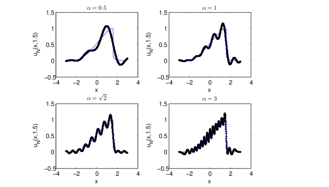
Figure 4.1: Solid blue line: the exact solution of Burger’s equation; Dotted line: the scheme (1.3) with $\epsilon_{N}=0$ (without viscosity) and $N=30$.

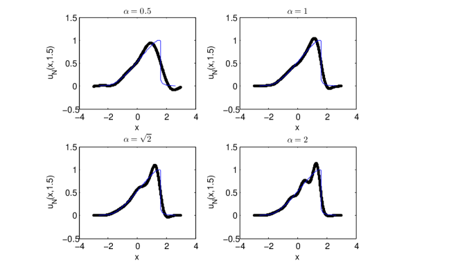
Figure 4.2: Solid blue line: the exact solution of Burger’s equation; dotted line: the scheme (1.3) with $\epsilon_{N}=0.5N^{-0.33}$ and $N=30$.

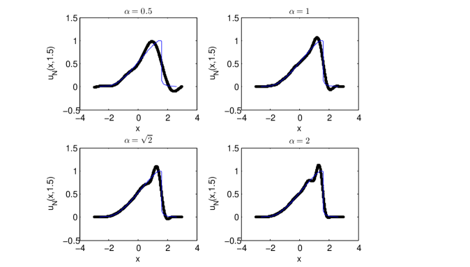
Figure 4.3: Solid blue line: the exact solution of Burger’s equation; dotted line: the scheme (1.3) with $\epsilon_{N}=0.5N^{-0.33}$ and $N=30$.

Figure 4.4: Solid blue line: the exact solution of Burger’s equation; dotted line: the scheme (1.3) with $\epsilon_{N}=0.5N^{-0.33}$ and $N=30$.

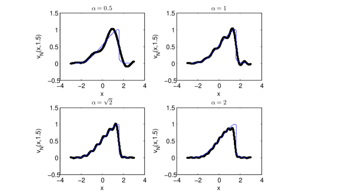
Figure 4.5: Solid blue line: the exact solution of Burger’s equation; dotted line: the scheme (1.6) with $\epsilon_{N}=0.05N^{-0.33}$ and $N=30$.

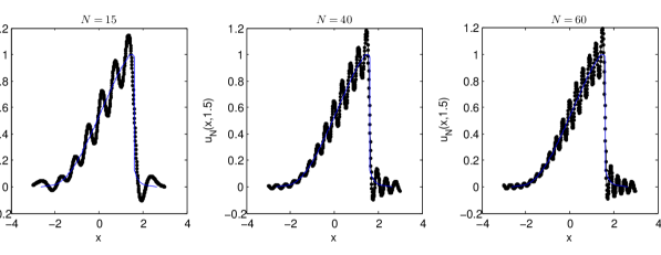
Figure 4.6: Solid blue line: the exact solution of Burger’s equation; dotted line: the approximate solution of the spectral scheme (1.3) with $\alpha=2$, $\epsilon_{N}=0$, $N=15,40$ and $60$, respectively.

4.2 Experiments with various $N$

In Figure 4.6, we show the result of the spectral approximation without viscosity, i.e. scheme (1.3) with $\epsilon_{N}=0$, $\alpha=2$, for $N=15,40$ and $60$, respectively. The larger $N$ is, the better resolution at the point of discontinuity we achieve, but the oscillations do not disappear as $N$ increases. The Gibb’s phenomenon prevents the convergence, even in the intervals where the exact solution is actually smooth. Compared with the pseudospectral viscosity method in [1] (cf. Figure 6.1), the discontinuity can be resolved by our scheme better with much smaller $N$, with the help of the scaling factor.

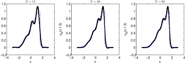
Figure 4.7: Solid blue line: the exact solution of inviscid Burger’s equation; dotted line: the approximate solution of the spectral scheme (1.3) with $\alpha=2$, $\epsilon_{N}=0.5N^{-0.33}$, $m_{N}=\lfloor{5N^{0.16}}\rfloor$, ${\hat{q}_{k}^{1}}$ and $N=15,40,60$.

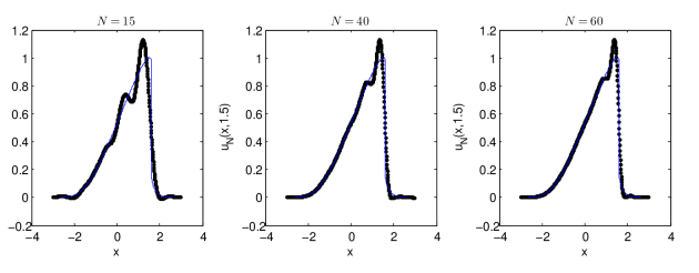
Figure 4.8: Solid blue line: the exact solution of inviscid Burger’s equation; dotted line: the approximate solution of the spectral scheme (1.3) with $\alpha=2$, $\epsilon_{N}=0.5N^{-0.33}$, $m_{N}=\lfloor{5N^{0.16}}\rfloor$, ${\hat{q}_{k}}^{2}$ and $N=15,40,60$.

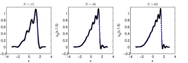
Figure 4.9: Solid blue line: the exact solution of inviscid Burger’s equation; dotted line: the approximate solution of the spectral scheme (1.3) with $\alpha=2$, $\epsilon_{N}=0.5N^{-0.33}$, $m_{N}=\lfloor{5N^{0.16}}\rfloor$, ${\hat{q}_{k}}^{3}$ and $N=15,40,60$.

In Figure 4.7-4.9, we add the viscosity term $\hat{q}_{k}^{1}-\hat{q}_{k}^{3}$ in (4) by suitably tuning the parameters $\epsilon_{N}=0.5N^{-0.33}$ and $m_{N}=\lfloor{5N^{0.16}}\rfloor$ with $N=15,40$ and $60$, respectively, where $\lfloor{\circ}\rfloor$ means the largest integer less than or equal to $\circ$. Compared with Figure 6.2 in [1], Figure 4.7-4.9 show the similar situation with various $\hat{q}_{k}$. That it, the approximate solution with the least oscillations is given by the scheme (1.3) with $\hat{q}_{k}^{2}$, while the best resolution of the shock is presented by that with $\hat{q}_{k}^{3}$. The conditions on $m_{N},\epsilon_{N}$ in Theorem 3.1 are satisfied. Clearly, the convergence of the approximate solution is better than that without viscosity. No matter what $\hat{q}_{k}$ is, the oscillations do not alleviate as $N$ increases, but the discontinuity is resolved better with larger $N$. Table 4.1 list $||\mathcal{D}_{x}u_{N}||^{2}_{L^{2}(0,T;L^{2}(\mathbb{R}))}$, $||xu_{N}||^{2}_{L^{2}(0,T;L^{2}(\mathbb{R}))}$ and $||u_{N}||^{2}_{L^{2}(0,T;L^{2}(\mathbb{R}))}$ versus $N$, where the approximate solution $u_{N}$ is obtained by the spectral scheme (1.3) with $\hat{q}_{k}^{1}$, $\alpha=\sqrt{2}$, $\epsilon_{N}=0.5N^{-0.33}$. It is used to numerically verify the condition (3.9) and the apriori estimate on $||\mathcal{D}_{x}Q_{m_{N}}u_{N}||_{L^{2}(0,T;L^{2}(\mathbb{R}))}^{2}$ (3.10). The norm $||\circ||_{L^{2}(\mathbb{R})}^{2}(t)$ at every time step is computed on the frequency side by Parseval’s identity, and the integration in time in $||\circ||_{L^{2}(0,T;L^{2}(\mathbb{R}))}$ is performed by the trapezoid rule. The time steps are given by the adaptive algorithm ode45 in Matlab. The command “polyfit” in Matlab is used to find the minimal mean square linear fit of the growth rate of $||\mathcal{D}_{x}u_{N}||_{L^{2}(0,T;L^{2}(\mathbb{R}))}^{2}$, $||xu_{N}||_{L^{2}(0,T;L^{2}(\mathbb{R}))}^{2}$ and $||u_{N}||_{L^{2}(0,T;L^{2}(\mathbb{R}))}^{2}$ with respect to $N$, which are $N^{0.1420},N^{-0.0049}$ and $N^{0.0007}$, respectively. It numerically confirms that $||xu_{N}||_{L^{2}(0,T;L^{2}(\mathbb{R}))}^{2}\lesssim N^{-0.0049}$, which can be interpreted as upper bound independent of $N$, i.e. condition (3.9) is satisfied. $||\mathcal{D}_{x}Q_{m_{N}}u_{N}||_{L^{2}(0,T;L^{2}(\mathbb{R}))}^{2}\lesssim N^{0.1420}+m_{N}N^{0.0007}\lesssim N^{0.1420}+N^{2*0.16+0.0007}\ll\frac{1}{\epsilon_{N}}\approx N^{0.33}$, that is, the apriori estimate (3.10) is correct.

N	40	45	50	55	60	65	70
$||\mathcal{D}_{x}u_{N}||_{L^{2}(0,T;L^{2}(\mathbb{R}))}^{2}$	$3.0621$	$3.1076$	$3.1504$	$3.1926$	$3.2350$	$3.2766$	$3.3145$
$||xu_{N}||_{L^{2}(0,T;L^{2}(\mathbb{R}))}^{2}$	$0.9690$	$0.9682$	$0.9676$	$0.9671$	$0.9667$	$0.9665$	$0.9664$
$||u_{N}||_{L^{2}(0,T;L^{2}(\mathbb{R}))}^{2}$	$1.8756$	$1.8757$	$1.8758$	$1.8759$	$1.8760$	$1.8762$	$1.8763$

Table 4.1: $||\mathcal{D}_{x}u_{N}||_{L^{2}(0,T;L^{2}(\mathbb{R}))}^{2}$, $||xu_{N}||_{L^{2}(0,T;L^{2}(\mathbb{R}))}^{2}$ and $||u_{N}||_{L^{2}(0,T;L^{2}(\mathbb{R}))}^{2}$ versus $N$, respectively, are displayed, where $u_{N}$ is the solution obtained by the spectral viscosity method (1.3) with $\hat{q}_{k}^{1}$, $\epsilon_{N}=0.5N^{-0.33}$.

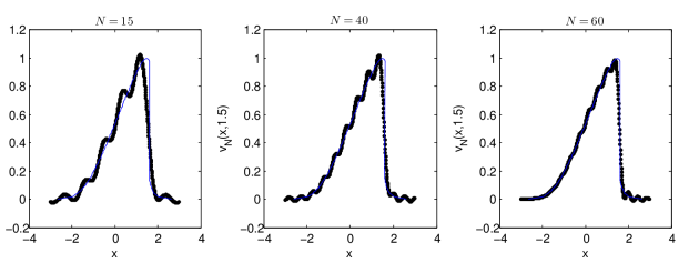
Figure 4.10: Solid blue line: the exact solution of inviscid Burger’s equation; dotted line: the approximate solution of the spectral scheme (1.6) with $\epsilon_{N}=0.05N^{-0.33}$, $\alpha=\sqrt{2}$ and $N=15,40,60$.

N	40	45	50	55	60	65	70
$||\mathcal{D}_{x}v_{N}||_{L^{2}(0,T;L^{2}(\mathbb{R}))}^{2}$	$4.4442$	$4.5220$	$4.5099$	$4.4977$	$4.6272$	$4.9252$	$5.1875$
$||v_{N}||^{2}_{L^{2}(0,T;L^{2}(\mathbb{R}))}$	$1.8829$	$1.8824$	$1.8814$	$1.8805$	$1.8804$	$1.8812$	$1.8819$
$||x^{2}v_{N}||_{L^{1}(\mathbb{R}\times(0,T))}$	$1.9499$	$1.9153$	$1.8911$	$1.8671$	$1.8657$	$1.8844$	$1.8791$

Table 4.2: $||\mathcal{D}_{x}v_{N}||_{L^{2}(0,T;L^{2}(\mathbb{R}))}^{2}$, $||v_{N}||_{L^{2}(0,T;L^{2}(\mathbb{R}))}^{2}$ and $||x^{2}v_{N}||_{L^{1}(\mathbb{R}\times(0,T))}$ versus $N$, respectively, are displayed, where $u_{N}$ is the solution obtained by the spectral viscosity method (1.6) with $\epsilon_{N}=0.05N^{-0.33}$.

Figure 4.5 reveals that the best resolution is obtained when $\alpha=\sqrt{2}$. Thus, we choose $\alpha=\sqrt{2}$ in the experiment of the scheme (1.6). Figure 4.10 displays the results of the spectral scheme (1.6) with $\epsilon_{N}=0.05N^{-0.33}$, $\alpha=\sqrt{2}$ and $N=15,40,60$. It shows that the larger $N$ is, the better resolution at discontinuity is obtained. In Table 4.2 we display $||\mathcal{D}_{x}v_{N}||_{L^{2}(0,T;L^{2}(\mathbb{R}))}^{2}$, $||v_{N}||_{L^{2}(0,T;L^{2}(\mathbb{R}))}^{2}$ and $||x^{2}v_{N}||_{L^{1}(\mathbb{R}\times(0,T))}$ versus $N$, respectively, where $v_{N}$ is the numerical solution to (1.6) with $\epsilon_{N}=0.05N^{-0.33}$. The norm $||\circ||_{L^{2}(0,T;L^{2}(\mathbb{R}))}^{2}$ is computed using the same rule as before. The integration in $||x^{2}v_{N}||_{L^{1}(\mathbb{R}\times(0,T))}$ is computed by trapezoid rule using equidistant grid. Again, we obtain the growth rate of $||\mathcal{D}_{x}v_{N}||_{L^{2}(0,T;L^{2}(\mathbb{R}))}^{2}$, $||v_{N}||_{L^{2}(0,T;L^{2}(\mathbb{R}))}^{2}$ and $||x^{2}v_{N}||_{L^{1}(\mathbb{R}\times(0,T))}$ versus $N$ by using “polyfit” in Matlab, which are $N^{0.2431},N^{-0.0014}$ and $N^{-0.0639}$, respectively. The condition (3.36) has been numerically verified.

4.3 Different $\epsilon_{N}$

It is natural to ask how to tune $\epsilon_{N}$ in our scheme (1.3). We need to balance the resolution near the discontinuity and the oscillations away from the discontinuity in the choice of $\epsilon_{N}$. With $N=40$, $\alpha=\sqrt{2}$ and $\hat{q}_{k}^{1}$, the results with $\epsilon_{N}=0.5N^{-0.9},0.5N^{-0.33}$ and $0.5N^{-0.001}$ are plotted in Figure 4.11. It is not surprising that (1.3) with $\epsilon_{N}=0.5N^{-0.9}$ does not converge, due to the violation of condition $N^{-\frac{1}{2}}\ll\epsilon_{N}\ll N^{-2\theta}$, $0<\theta<\frac{1}{4}$ in Theorem 3.1, cf. Figure 4.11. We expect that the larger $\epsilon_{N}$ will give a smoother approximate solution. However, as shown in Figure 4.11, it is not the case, that is, the approximate solution with $\epsilon_{N}=0.5N^{-0.33}$ yields fewer oscillations than that with $\epsilon_{N}=0.5N^{-0.001}$. Similar situation can also be observed in Figure 4.12-4.13, where the scheme (1.3) with $\hat{q}_{k}^{2}$ and $\hat{q}_{k}^{3}$ instead.

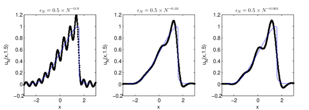
Figure 4.11: Solid blue line: the exact solution of inviscid Burger’s equation; dotted line: the spectral scheme (1.3) with $N=40$, $\alpha=\sqrt{2}$, $\hat{q}_{k}^{1}$ and $\epsilon_{N}=0.5N^{-0.9},0.5N^{-0.33},0.5N^{-0.001}$.

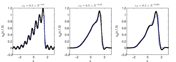
Figure 4.12: Solid blue line: the exact solution of inviscid Burger’s equation; dotted line: the spectral scheme (1.3) with $N=40$, $\alpha=\sqrt{2}$, $\hat{q}_{k}^{2}$ and $\epsilon_{N}=0.5N^{-0.9},0.5N^{-0.33},0.5N^{-0.001}$.

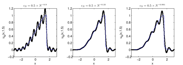
Figure 4.13: Solid blue line: the exact solution of inviscid Burger’s equation; dotted line: the spectral scheme (1.3) with $N=40$, $\alpha=\sqrt{2}$, $\hat{q}_{k}^{3}$ and $\epsilon_{N}=0.5N^{-0.9},0.5N^{-0.33},0.5N^{-0.001}$.

5 Conclusion

In this paper, we propose two spectral viscosity methods based on the generalized Hermite functions for the solution of nonlinear scalar conservation laws in the whole line. Our schemes have been shown rigorously that the approximate solutions converge to the unique entropy solution by using compensated compactness arguments. The numerical experiments of the inviscid Burger’s equation illustrate the implementability of our schemes. Thanks to the generalized Hermite functions, the approximate solutions of our scheme have fewer oscillations and better resolutions of the discontinuity, with much smaller truncation modes $N$, compared with those in [1], even before adding the viscosity term.

References

- [1] J. Aguirre and J. Rivas, A spectral viscosity method based on Hermite functions for nonlinear conservations laws, SIAM J. Numer. Anal., 46(2): 1060-1078, 2008.
- [2] J. Boyd, The rate of convergence of Hermite function series, Math. Comp., 35:1039-1316, 1980.
- [3] J. Boyd, Asymptotic coefficients of Hermite function series, J. Comput. Phys., 54:382-410, 1984.
- [4] J. Boyd, Chebyshev and Fourier Spectral Methods, 2d. edition, Dover, New York, 2001
- [5] G.-Q. Chen, The compensated compactness method and the system of isentropic gas dynamics, Preprint MSRI-00527-91, Mathematical Science Research Institute, Berkeley, CA, 1990.
- [6] G.-Q. Chen, Q. Du and E. Tadmor, Spectral viscosity approximations to multidimensional scalar conservation laws, Math. Comp., 61:629-643, 1993.
- [7] D. Funaro and O. Kavian, Approximation of some diffusion evolution equation in unbounded domains by Hermite function, Math. Comp., 37:597-619, 1991.
- [8] A. Gelb and E. Tadmor, Enhanced spectral viscosity approximations for conservation laws, Appl. Numer. Math., 33:3-21, 2000.
- [9] D. Gottlieb and S. Orszag, Numerical analysis of spectral methods: theory and applications, Soc. In. and Appl. Math., Philadelphia, 1977.
- [10] D. Gottlieb and C.-W. Shu, On the Gibbs phenomenon and its resolution, SIAM Rev., 39(4):644-668, 1997.
- [11] D. Gottlieb, C.-W. Shu, A. Solomonoff, and H. Vandeven, On the Gibbs phenomenon I: Recovering exponential accuracy from the Fourier partial sum of a nonperiodic analytic function, J. Comput. Appl. Math., 43:81-92, 1992.
- [12] D. Gottlieb and E. Tadmor, Recovering pointwise values of discontinuous data within spectral accuracy, in Progress and Supercomputing in Computational Fluid Dynamics, E. M. Murman and S. S. Abarbanel, eds., Birkhäuser, Boston, 357-275, 1985.
- [13] B.-Y. Guo, H. Ma, and E. Tadmor, Spectral vanishing viscosity method for nonlinear conservation laws, SIAM J. Numer. Anal., 39(4):1254-1268, 2001.
- [14] X. Luo and S. S.-T. Yau, Hermite spectral method to 1D forward Kolmogorov equation and its application to nonlinear filtering problems, IEEE Trans. Automat. Control, 58(10):2495-2507, 2013.
- [15] X. Luo, S.-T. Yau and S. S.-T, Yau, Time-dependent Hermite-Galerkin spectral method and its applications, Appl. Math. Comput., 264:378-391, 2015.
- [16] H. Ma, Chebyshev-Legendre spectral viscosity method for nonlinear conservation laws, SIAM J. Numer. Anal., 35(3):869-892, 1998.
- [17] H. Ma, Chebyshev-Legendre super spectral viscosity method for nonlinear conservation laws, SIAM J. Numer. Anal., 35(3):893-908, 1998.
- [18] Y. Maday, S. M. Ould Kaber, and E. Tadmor, Legendre pseudospectral viscosity method for nonlinear conservation laws, SIAM J. Numer. Anal., 30:321-342, 1993.
- [19] Y. Maday and E. Tadmor, Analysis of the spectral vanishing viscosity method for periodic conservation laws, SIAM J. Numer. Anal., 26:854-870, 1989.
- [20] S. Schochet, The rate of convergence of spectral-viscosity methods for periodic scalar conservation laws, SIAM J. Numer. Anal., 27:1142-1159, 1990.
- [21] J. Smoller, Shock waves and reaction-diffusion equations, Springer-Verlag, New York, 1983.
- [22] J. Shen, T. Tang and L.-L. Wang, Spectral Methods: Algorithm, Analysis and Application, Springer, 2011.
- [23] J. Shen and L.-L. Wang, Some recent advances on spectral methods fo unbounded domains, Commun. Comput. Phys., 5:195-241, 2009.
- [24] E. Tadmor, Convergence of spectral methods for nonlinear conservation laws, SIAM J. Numer. Anal., 26:30-44, 1989.
- [25] E. Tadmor, Shock capturing by the spectral viscosity method, Comput. Methods Appl. Mech. Engrg., 80:197-208, 1990.
- [26] T. Tang, The Hermite spectral method for Gaussian-type functions, SIAM J. Sci. Comput., 14:594-606, 1993.
- [27] L. Tartar, Compensated compactness and applications to partial differential equations, in Nonlinear Analysis and Mechanics: Heriot-Watt Symposium, Vol. IV, Res. Notes n Math. 39:136-212, J. Knopps, ed., Pitman, Boston, London, 1979.
- [28] H. Vandeven, Family of spectral filters for discontinuous problems, J. Sci. Comput., 8:159-192, 1991.
- [29] X.-M. Xiang and Z.-Q. Wang, Generalized Hermite spectral method and its applications to problems in unbounded domains, SIAM J. Numer. Anal., 48(4):1231-1253, 2010.