Turing degrees of limit sets of cellular automata

Abstract

Cellular automata are discrete dynamical systems and a model of computation. The limit set of a cellular automaton consists of the configurations having an infinite sequence of preimages. It is well known that these always contain a computable point and that any non-trivial property on them is undecidable. We go one step further in this article by giving a full characterization of the sets of Turing degrees of cellular automata: they are the same as the sets of Turing degrees of effectively closed sets containing a computable point.

1 Introduction

Cellular Automata (CAs for short) are both discrete dynamical systems and a model of computation. They were introduced in the late 1940s independently by John von Neumann and Stanislaw Ulam to study, respectively, self-replicating systems and the growth of quasi-crystals.

A $d$-dimensional CA consists of cells aligned on ${\mathbb{Z}^{d}}$ that may be in a finite number of states, and are updated synchronously with a local rule, i.e. depending only on a finite neighborhood. All cells operate under the same local rule. The state of all cells at some time step is called a configuration. CAs are very well known for being simple systems that may exhibit complicated behavior.

A $d$-dimensional subshift of finite type (SFT for short) is a set of colorings of ${\mathbb{Z}^{d}}$ by a finite number of colors containing no pattern from a finite family of forbidden patterns. Most proofs of undecidability concerning CAs involve the use of SFTs, so both topics are very intertwined [Kar90, Kar92, Kar94, Mey08, Kar11]. A recent trend in the study of SFTs has been to give computational characterizations of dynamical properties, which has been followed by the study of their computational structure and in particular the comparison with the computational structure of effectively closed sets, which are the subsets of $\left\{0,1\right\}^{\mathbb{N}}$ on which some Turing machine does not halt. It is quite easy to see that SFTs are such sets.

In this paper, we follow this trend and study the limit set $\Omega\left(\mathcal{A}\right)$ of a CA $\mathcal{A}$, which consist of all the configurations of the CA that can occur after arbitrarily long computations. They were introduced by [CPY89] in order to classify CAs. It has been proved that non-trivial properties on these sets are undecidable by [Kar94a, GR10] for CAs of all dimensions. Limit sets of CAs are subshifts, and the question of which subshifts may be limit sets of CA has been a thriving topic, see [Hur87, Hur90, Hur90a, Maa95, FK07, LM09, BGK11]. However, most of these results are on the language of the limit set or on simple limit sets. Our aim here is to study the configurations themselves.

In dimension $1$, limit sets are effectively closed sets, so it is quite natural to compare them from a computational point of view. The natural measure of complexity for effectively closed sets is the Medvedev degree [Sim11], which, informally, is a measure of the complexity of the simplest points of the set. As limit sets always contain a uniform configuration (wherein all cells are in the same state), they always contain a computable point and have Medvedev degree $\mathbf{0}$. Thus, if we want to study their computable structure, we need a finer measure; in this sense, the set of Turing degrees is appropriate.

It turns out that for SFTs, there is a characterization of the sets of Turing degrees found by [JV13a], which states that one may construct SFTs with the same Turing degrees as any effectively closed set containing a computable point. In the case of limit sets, such a characterization would be perfect, as limit sets always contain a computable point. This is exactly what we achieve in this article:

Theorem 1.

For any effectively closed set $S$, there exists a cellular automaton $\mathcal{A}$ such that

$${\deg_{T}}\Omega\left(\mathcal{A}\right)={\deg_{T}}{S}\cup\{{\mathbf{0}}\}\text{.}$$

In the way to achieve this theorem, we introduce a new construction which gives us some control over the limit set. We hope that this construction will lead to other unrelated results on limit sets of CAs, as it was the case for the construction in [JV13a], see [JV13].

The paper is organized as follows. In Section 2 we recall the usual definitions concerning CAs and Turing degrees. In Section 3 we give the reasons for each trait of the construction which allows us to prove theorem 1. In Section 4 we give the actual construction. We end the paper by a discussion, in Section 5, on the Cantor-Bendixson ranks of the limit sets of CAs. The choice has been made to have colored figures, which are best viewed on screen.

2 Preliminary definitions

A ($1$-dimensional) cellular automaton is a triple $\mathcal{A}=(Q,r,\delta)$, where $Q$ is the finite set of states, $r>0$ is the radius and $\delta:Q^{2r+1}\to Q$ the local transition function.

An element of $i\in\mathbb{Z}$ is called a cell, and the set $\llbracket i-r,i+r\rrbracket$ is the neighborhood of $i$ (the elements of which are the neighbors of $i$). A configuration is a function $\mathfrak{c}:\mathbb{Z}\to Q$. The local transition function induces a global transition function (that can be regarded as the automaton itself, hence the notation), which associates to any configuration $\mathfrak{c}$ its successor:

$$\mathcal{A}(\mathfrak{c}):\left\{\begin{array}[]{ccl}\mathbb{Z}&\to&Q\\ i&\mapsto&\delta(\mathfrak{c}(i-r),\dots,\mathfrak{c}(i-1),\mathfrak{c}(i),\mathfrak{c}(i+1),\dots,\mathfrak{c}(i+r)))\text{.}\end{array}\right.$$

In other words, all cells are finite automata that update their states in parallel, according to the same local transition rule, transforming a configuration into its successor.

If we draw some configuration as a horizontal bi-infinite line of cells, then add its successor above it, then the successor of the latter and so on, we obtain a space-time diagram, which is a two-dimensional representation of some computation performed by $\mathcal{A}$.

A site $(i,t)\in\mathbb{Z}^{2}$ is a cell $i$ at a certain time step $t$ of the computation we consider (hereinafter there will never be any ambiguity on the automaton nor on the computation considered).

The limit set of $\mathcal{A}$, denoted by $\Omega\left(\mathcal{A}\right)$, is the set of all the configurations that can appear after arbitrarily many computation steps:

$$\Omega\left(\mathcal{A}\right)=\bigcap_{k\in\mathbb{N}}\mathcal{A}^{k}(Q^{\mathbb{Z}})\text{.}$$

For surjective CAs, the limit set is the set of all possible configurations $Q^{\mathbb{Z}}$, while for non-surjective CAs, it is the set of all configurations containing no orphan of any order, see [Hur90]. An orphan of order $n$ is a finite word $w$ which has no preimage by $\mathcal{A}^{n}_{|Q^{|w|}}$.

An effectively closed set, or $\Pi^{0}_{1}$ class, is a subset $S$ of $\left\{0,1\right\}^{\mathbb{N}}$ for which there exists a Turing machine that, given any $x\in\left\{0,1\right\}^{\mathbb{N}}$, halts if and only if $x\not\in S$. Equivalently, a class $S\subseteq\left\{0,1\right\}^{\mathbb{N}}$ is $\Pi^{0}_{1}$ if there exists a computable set $L$ such that $x\in S$ if and only if no prefix of $x$ is in $L$. It is then quite easy to see that limit sets of CAs are $\Pi^{0}_{1}$ classes: for any limit set, the set of forbidden patterns is the set of all orphans of all orders, which form a recursively enumerable set, since it is computable to check whether a finite word is an orphan.

For $x,y\in\left\{0,1\right\}^{\mathbb{N}}$, we say that $x{\leq_{T}}y$ if $x$ is computable by a Turing machine using $x$ as an oracle. If $x{\leq_{T}}y$ and $x{\geq_{T}}y$, $x$ and $y$ are said to be Turing-equivalent, which is noted $x{\equiv_{T}}y$. The Turing degree of $x$, noted ${\deg_{T}}x$, is its equivalence class under relation ${\equiv_{T}}$. The Turing degrees form a lattice whose bottom is $\mathbf{0}$, the Turing degree of computable sequences.

Effectively closed sets are quite well understood from a computational point of view, and there has been numerous contributions concerning their Turing degrees, see the book of [CR98] for a survey. One of the most interesting results may be that there exist $\Pi^{0}_{1}$ classes whose members are two-by-two Turing incomparable [JS72].

3 Requirements of the construction

The idea to prove Theorem 1 is to make a construction that embeds computations of a Turing machine that will check a read-only oracle tape containing a member of the $\Pi^{0}_{1}$ class $S$ that will have to appear “non-deterministically”. The following constraints have to be addressed.

• Since CAs are intrinsically deterministic, this non-determinism will have to come from the “past”, i.e. from the “limit” of the preimages.

• The oracle tape, the element of $\left\{0,1\right\}^{\mathbb{N}}$ that needs to be checked, needs to appear entirely on at least one configuration of the limit set.

• Each configuration of the limit set containing the oracle tape needs to have exactly one head of the Turing machine, in order to ensure that there really is a computation going on in the associated space-time diagram.

• The construction, without any computation, needs to have a very simple limit set, i.e. it needs to be computable, and in particular countable; this to ensure that no complexity overhead will be added to any configuration containing the oracle tape, and that “unuseful” configurations of the limit set – the configurations that do not appear in a space-time diagram corresponding to a computation – will be computable.

• The computation of the embedded Turing machine needs to go backwards, this to ensure that we can have the non-determinism. And an error in the computation must ensure that there is no infinite sequence of preimages.

• The computation needs to have a beginning (also to ensure the presence of a head), so the construction needs some marked beginning, and the representation of the oracle and work tapes in the construction need to disappear at this point, otherwise by compactness the part without any computation could be extended bi-infinitely to contain any member of $\left\{0,1\right\}^{\mathbb{N}}$, thus leading to the full set of Turing degrees.

There are other constraints that we will discuss during the construction, as they arise.

In order to make a construction complying to all these constraints, we reuse, with heavy modifications, an idea of [JV13a], which is to construct a sparse grid. However, their construction, being meant for subshifts, requires to be completely rethought in order to work for CAs. In particular, there was no determinism in this construction, and the oracle tape did not need to appear on a single column/row, since their result was on two-dimensional subshifts.

4 The construction

4.1 A self-vanishing sparse grid

In order to have space-time diagrams that constitute sparse grids, the idea is to have columns of squares, each of these columns containing less and less squares as we move to the left, see fig. 1. The CA has three categories of states:

• a killer state, which is a spreading state that erases anything on its path;

• a quiescent state, represented in white in the figures; its sole purpose is to mark the spaces that are “outside” the construction;

• some construction states, which will be constituted of signals and background colors.

In order to ensure that just with the signals themselves it is not possible to encode anything non-computable in the limit set, all signals will need to have, at all points, at any time, different colors on their left and right, otherwise the local rule will have a killer state arise. Here are the main signals.

• Vertical lines: serve as boundaries between columns of squares and form the left/right sides of the squares.

• SW-NE and SE-NW diagonals: used to mark the corners of the squares, they are signals of respective speeds $1$ and $-1$. Each time they collide with a vertical line (except for the last square of the row), they bounce and start the converse diagonal of the next square.

• Counting signal: will count the number of squares inside a column; every time it crosses the SW-NE diagonal of a square it will shift to the left. When it is superimposed to a vertical line, it means that the square is the last of its column, so when it crosses the next SE-NW diagonal, it vanishes and with it the vertical line.

• Starting signals: used to start the next column to the left, at the bottom of one column. Here is how they work.

  • The bottommost signal, of speed $-\frac{1}{4}$, is at the boundary between the empty part of the space-time diagram and the construction. It is started $4$ time steps after the collision with the signal of speed $-\frac{1}{3}$.

  • The signal of speed $-\frac{1}{3}$ is started just after the vertical line sees the incoming SE-NW diagonal of the first square of the row on the right, at distance $3$ (the diagonal will collide with the vertical line $2$ time steps after the start of that signal).

  • At the same time as the signal of speed $-\frac{1}{3}$ is created, a signal of speed $-\frac{1}{2}$ is generated. When this signal collides with the bottommost signal, it bounces into a signal of speed $\frac{1}{4}$ that will create the first SE-NW diagonal of the first square of the row of squares of the left, $4$ time steps after it will collide with the vertical line.

On top of the construction states, except on the vertical lines, we add a parity layer $\{0,1\}$: on a configuration, two neighboring cells of the construction must have different parity bits, otherwise a killer state appears. On the left of a vertical line there has to be parity $1$ and on the right parity $0$, otherwise the killer state pops up again. This is to ensure that the columns will always contain an even number of squares.

Figure 1: The sparse grid construction: it is based on columns containing a finite number of squares, whose number decreases when we go left. Note that the figure is squeezed vertically.

The following lemmas address which types of configurations may occur in the limit set of this CA. First note that any configuration wherein the construction states do not appear in the right order do not have a preimage.

Lemma 4.1.

The sequence of preimages of a segment ended by consecutive vertical lines (and containing none) is a slice of a column of squares of even side.

Proof.

Suppose a configuration contains two vertical-line symbols, then to be in the limit set, in between these two symbols there needs to be two diagonal symbols, one for the SE-NW one and one for SW-NE one, a symbol for the counting signal, and in between these signals there needs to be the appropriate colors: there is only one possibility for each of them. If this is not the case, then the configuration has no preimage.

Also, the distance between the first vertical line and the SE-NW diagonal needs to be the same than the distance between the second vertical line and the SW-NE diagonal, otherwise the signals at the bottom – the ones starting a column, that are the only preimages of the first diagonals – would have, in one case, created a vertical line in between, and in the other case, not started at the same time on the right vertical.

The side of the squares is even, otherwise the parity layer has no preimage.∎

Lemma 4.2.

A configuration of the limit set containing at least three vertical-line symbols needs to verify, for any three consecutive symbols, that if the distance between the first one and the second one is $k$, then the distance between the second one and the third one needs to be $(k+2)$.

Proof.

Let us take a configuration containing at least three vertical-line symbols, take three consecutive ones. The states between them have to be of the right form as we said above. Suppose the first of these symbols is at distance $k_{1}$ of the second one, which is at distance $k_{2}$ of the third one. This means that the first (resp. second) segment defines a column of squares of side $k_{1}$ (resp. $k_{2}$). It is clear that the second column of squares cannot end before the first one.

Now let $i$ be the position of the counting signal of the first column and $j$ the distance between the SW-NE diagonal and the left vertical line. The preimage of the first segment ends $(k_{1}i+j)$ (resp. $(k_{1}(i-1)+j)$) steps before if the counting signal is on the left (resp. right) of the SW-NE diagonal. Then, the preimages of the left and right vertical lines of this column are the creating signals. Before the signal created on the right bounces on the one of speed $-\frac{1}{4}$ created on the left, it collides with the one of speed $-\frac{1}{3}$, thus determining the height of the squares on the right column of squares. So $k_{1}=k_{2}-2$. ∎

Lemma 4.3.

A configuration having two vertical-line symbols pertaining to the limit set needs to verify one of the following statements.

• It is constituted of a finite number of vertical lines.

• It appears in the space-time diagram of fig. 1.

• It is constituted of an infinite number of vertical lines, then starting from some position it is equal on the right to some (shifted) line of fig. 1.

Proof.

We place ourselves in the case of a configuration of the limit set. Because of lemma 4.1, two consecutive vertical lines at distance $k$ from each other define a column of squares. In a space-time diagram they belong to, on their left there necessarily is another column of squares, because of the starting signal generated at the beginning of the left vertical line, except when $k=3$, in which case there is nothing on the left. In this column, the vertical lines are at distance $(k-2)$, see lemma 4.2. So, if there is an infinite number of vertical lines, either it is of the form of fig. 1, or there is some killer state coming from infinity on the left and “eating” the construction. ∎

4.2 Backward computation inside the grid

We now wish to embed the computation of a reversible Turing machine inside the aforementioned sparse grid, which for this purpose is better seen as a lattice. The fact the TM is reversible allows us to embed it backwards in the CA. We will below denote by TM time (resp. CA time) the time going forward for the Turing machine (resp. the CA); on a space-time diagram, TM time goes from top to bottom, while CA time goes from bottom to top (cf. arrows in fig. 2a). That way, the beginning of the computation of the TM will occur in the first (topmost) square of the first (leftmost) column of squares.

We have to ensure that any computation of the TM is possible, and in particular ensure that such a computation is consistent over time; the idea is that at the first TM time step, i.e. the moment the sparse grid disappears, the tape is on each of the vertical line symbols, but since these all disappear a finite number of CA steps before, we have to compel all tape cells to shift to the right regularly as TM time increases.

Moreover, we want to force the presence of exactly one head (there could be none if it were, for instance, infinitely far right). To do that, the grid is divided into three parts that must appear in this order (from left to right): the left of the head, the right of the head (together referred to as the computation zone) and the unreachable zone (where no computation can ever be performed), resp. in blue, yellow and green in fig. 2a.

The vertices of our lattice are the top left corners of the squares, each one marked by the rebound of a SE-NW diagonal on a vertical line, while the top right corners will just serve as intermediate points for signals. More precisely, if we choose (arbitrarily) the top left corner of the first square of the first column to appear at site $(0,0)$, then for any $i,j\in\mathbb{N}$, the respective sites for the top left and top right corners of $s_{i,j}$, the $(j+1)$-th square of the $(i+1)$-th column, are the following (cf. fig. 2a):

$$\left\{\begin{array}[]{ l@{\;}l@{\;}l}s^{\ell}_{i,j}&=&(i(i+1),-2(i+1)j)\\ s^{r}_{i,j}&=&((i+1)(i+2),-2(i+1)j)\text{.}\end{array}\right.$$

Fig. 2b illustrates a computation by the TM, with the three aforementioned zones, as it would be embedded the usual way (but with reverse time) into a CA, with site $(i,-t)$ corresponding to the content of the tape at $i\in\mathbb{N}$ and TM time $t\in\mathbb{N}$.

Fig. 2c represents another, still simple, embedding, which is a distortion of the previous one: the head moves every even time step within a tape that is shifted every odd time steps, so that instead of site $(i,-t)$, we have two sites, $(i+t,-2t)$ and $(i+t,-2t-1)$, resp. the computation site (big circle on fig. 2c) and the shifting site (small circle on fig. 2c). The head only reads the content of the tape when it lies on a computation site. This type of embedding can easily be realized forwards or backwards (provided the TM is reversible).

Our embedding, derived from the latter, is drawn on fig. 2a. The “only” difference is the replacement of sites $(i+t,-2t)$ and $(i+t,-2t-1)$ by sites $s^{\ell}_{i,t}$ and $s^{\ell}_{i,t+1}$. Notice that as the number of squares in a column is always finite, each square can “know” whether its top left corner is a computation or a shifting site with a parity bit. More precisely, the $j$-th square (from bottom to top) of a column has a computation site on its top left if and only if $j$ is even.

Let $s_{i,j}$ be a square of our construction. $s^{\ell}_{i,j}$ is either a computation site or a shifting site. In the latter case, it is supposed to receive the content of a cell of the TM tape with an incoming signal of speed $-1$. All it has to do is to send it to $s^{\ell}_{i,j-1}$ (at speed $0$), which is a computation site. In the former case, however, things a slightly more complicated. The content of the tape has to be transmitted to $s^{\ell}_{i-1,j-1}$ (which is a shifting site). To do that, a signal of speed $0$ is sent and waits for site $s^{r}_{i-1,j}$, which sends the content to $s^{\ell}_{i-1,j-1}$ with a signal of speed $-1$ along the SE-NW diagonal. The problem is to recognize which $s^{r}$ site is the correct one. Fortunately, there are only two possibilities: it is either the first or the second $s^{r}$ site to appear after (in CA time, of course) $s^{\ell}_{i,j}$ on the vertical line. The first case corresponds exactly to the unreachable zone (where $j\leq i$), hence the result if the three zones are marked. The lack of other cases is due to the number of $s_{i}$ squares, which is only $2(i+1)$.

Another issue is the superposition of such signals. Here again, there are only two cases: in the unreachable zone there is none, whereas in the computation zone a signal of speed $0$ from a computation site can be superimposed to the signal of speed $0$ sent by the shifting site just above it. As aforesaid, there is no other case because of the limited number of $s_{i}$ squares. Thus, there is no problem to keep the number of states of the CA finite, since the number of signals going through a same cell is limited to two at the same time.

While the two parts of the computation zones are to be separated by the presence of a head, the unreachable zone is at the right of a signal that is sent from any computation site that has two diagonals (one from the left and one from the right) below it (indicated as circles on fig. 1), goes at speed $0$ until the next $s^{r}$ site, then at speed $1$ (along SE-NW diagonals) to the second next shifting site, and finally at speed $0$ again, to the next computation site (cf. fig. 2a), which also has two diagonals below it if the grid contains no error. Another way to detect the unreachable zone is to detect that the counting signal crossed the SW-NE diagonal exactly two CA time steps after it has crossed the SE-NW diagonal. This means that the unreachable zone is structurally coded in the construction.

Now only the movements of the head remain to be described (in black on fig. 2a). Let $s^{\ell}_{i,j}$ be a computation site containing the head.

• If the previous move of the head (previous because we are in CA time, that is, in reverse TM time) was to the left, the next computation site is the one just above, that is, $s^{\ell}_{i,j-2}$. The head is thus transferred by a simple signal of speed $0$.

• If the previous move was to stand still, the next computation site is $s^{\ell}_{i-1,j-2}$. It can be reached by a signal of speed $0$ until the second next $s^{r}$ site, from which a signal of speed $-1$ (along a SE-NW diagonal) is launched, to be replaced by another signal of speed $0$ from $s^{\ell}_{i-1,j-1}$ on.

• If the previous move was to the right, the next computation site is $s^{\ell}_{i-2,j-2}$. It can be reached by a signal of speed $0$ until the second next $s^{r}$ site, from which a signal of speed $-1$ (along a SE-NW diagonal) is launched, to be replaced by another signal of speed $0$ from $s^{\ell}_{i-1,j-1}$ on, which itself waits for the next $s^{r}$ site (which is $s^{r}_{i-2,j}$) to start another signal of speed $1$ (along a SW-NE diagonal) that is finally succeeded to by a last signal of speed $0$ from $s^{\ell}_{i-2,j-1}$ on.

(a)

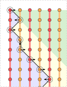
(b)

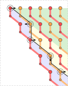
(c)

Figure 2: The embedding of a Turing machine computation in the sparse grid (2a), compared to the usual embedding (2b) and a slightly distorted one (2c). The paths followed by the content of each cell of the tape are in red and orange (two colors just to keep track of the signals), while the one of the head is in black. The arrows indicate the next move of the head (for TM time, going towards the bottom). The green background denotes the zone the head cannot reach, while the computation zone is in blue on the left of the head and in yellow on its right.

4.3 The computation itself

As we said before, the computation will take place on the computation sites, which will contain two kinds of tape cells: one for the oracle and one for the work. In the unreachable zone there are only oracle cells, which do not change over time except for the shifting. Now we want to eliminate all space-time diagrams corresponding to rejecting computations of some Turing machine $M$. [Ben73] has proved that for any Turing machine, we can construct a reversible one computing the same function. So a first idea would just be to encode this reversible Turing machine in the sparse grid; however there is no way to guarantee that the work tape that was non-deterministically inherited from the past corresponds to a valid configuration and by the time the Turing machine “realizes” this it will be too late, there will already exist configurations containing some oracle that we would otherwise have rejected.

The solution to this problem is to use a robust Turing machine in the sense of [Hoo66], that is to say a Turing machine that regularly rechecks its whole computation. [KO08] have constructed reversible such machines. In these constructions the machines constructed were working on a bi-infinite tape, which had the drawback that some infinite side of the tape might not be checked; here it is not the case, hence we can modify the machine so that on an infinite computation it visits all cells of the tape (we omit the details for brevity’s sake).

In terms of limit sets, this means that if some oracle is rejected by the machine, then it must have been rejected an infinite number of times in the past (CA time). So, only oracles pertaining to the desired class may appear in the limit set.

Furthermore, even if some killer state coming from the right eats the grid, at some point in the past of the CA, it will be in the unreachable zone, and stay there for ever, so the computation from that moment on even ensures that the oracle computed is correct. Though, that doesn’t matter, because in this case the configurations of the corresponding space-time diagram that are in the limit set are uniform both on the right and on the left except for a finite part in the middle, and are hence computable.

5 Cantor-Bendixson rank of limit sets

The Cantor-Bendixson derivative of some set $S\subseteq\Sigma^{\mathbb{Z}}$, with $\Sigma$ finite, is noted $\mathfrak{D}\left(S\right)$ and consists of all configurations of $S$ except the isolated ones. A configuration $\mathfrak{c}$ is said to be isolated if there exists a pattern $P$ such that $\mathfrak{c}$ is the only configuration of $S$ containing $P$ (up to a shift). For any ordinal $\lambda$ we can define ${S}^{\left(\lambda\right)}$, the Cantor-Bendixson derivative of rank $\lambda$, inductively:

$$\begin{array}[]{l@{\;\;}c@{\;\;\;}l}{S}^{\left(0\right)}&=&S\\ {S}^{\left(\lambda+1\right)}&=&\mathfrak{D}\left({S}^{\left(\lambda\right)}\right)\\ {S}^{\left(\lambda\right)}&=&\displaystyle{\bigcap_{\gamma<\lambda}}{S}^{\left(\gamma\right)}\text{.}\end{array}$$

The Cantor-Bendixson rank of $S$, denoted by $\mathfrak{CB}\left(S\right)$, is defined as the first ordinal  $\lambda$ such that ${S}^{\left(\lambda+1\right)}={S}^{\left(\lambda\right)}$. In particular, when $S$ is countable, ${S}^{\left(\mathfrak{CB}\left(S\right)\right)}$ is empty. An element $s$ is of rank $\lambda$ in $S$ if $\lambda$ is the least ordinal such that $s\notin{S}^{\left(\lambda\right)}$. For more information about Cantor-Bendixson rank, one may skim [Kec95].

The Cantor-Bendixson rank corresponds to the height of a configuration corresponding to a preorder on patterns as noted by [BDJ08].Thus, it gives some information on the way the limit set is structured pattern-wise. A straightforward corollary of the construction above is the following.

Corollary 5.1.

There exists a constant $c\leq 10$ such that for any $\Pi^{0}_{1}$ class $S$, there exists a CA $\mathcal{A}$ such that

$$\mathfrak{CB}\left(\Omega\left(\mathcal{A}\right)\right)=\mathfrak{CB}\left(S\right)+c\text{.}$$

Here the constant corresponds to the pattern overhead brought by the sparse-grid construction.

References

- [BDJ08] Alexis Ballier, Bruno Durand and Emmanuel Jeandel “Structural aspects of tilings” In 25th International Symposium on Theoretical Aspects of Computer Science 1, Leibniz International Proceedings in Informatics (LIPIcs) Dagstuhl, Germany: Schloss Dagstuhl–Leibniz-Zentrum fuer Informatik, 2008, pp. 61–72 DOI: http://dx.doi.org/10.4230/LIPIcs.STACS.2008.1334
- [Ben73] C. H. Bennett “Logical Reversibility of Computation” In IBM J. Res. Dev. 17.6 Riverton, NJ, USA: IBM Corp., 1973, pp. 525–532 DOI: 10.1147/rd.176.0525
- [BGK11] Alexis Ballier, Pierre Guillon and Jarkko Kari “Limit Sets of Stable and Unstable Cellular Automata” In Fundam. Inform. 110.1-4, 2011, pp. 45–57
- [CPY89] Karel Culik, J. Pachl and S. Yu “On the limit sets of cellular automata” In SIAM Journal on Computing 18.4, 1989, pp. 831–842
- [CR98] Douglas Cenzer and J.B. Remmel “ classes in mathematics” In Handbook of Recursive Mathematics - Volume 2: Recursive Algebra, Analysis and Combinatorics 139, Studies in Logic and the Foundations of Mathematics Elsevier, 1998, pp. 623–821 DOI: 10.1016/S0049-237X(98)80046-3
- [FK07] Enrico Formenti and Petr Kurka “Subshift attractors of cellular automata” In Nonlinearity 20, 2007, pp. 105–117
- [GR10] Pierre Guillon and Gaétan Richard “Revisiting the Rice Theorem of Cellular Automata” In STACS 5, LIPIcs Schloss Dagstuhl - Leibniz-Zentrum fuer Informatik, 2010, pp. 441–452
- [Hoo66] Philip K. Hooper “The Undecidability of the Turing Machine Immortality Problem” In Journal of Symbolic Logic 31.2, 1966, pp. 219–234
- [Hur87] Lyman P. Hurd “Formal Language Characterization of Cellular Automaton Limit Sets” In Complex Systems 1.1, 1987, pp. 69–80
- [Hur90] Lyman P. Hurd “Nonrecursive Cellular Automata Invariant Sets” In Complex Systems 4.2, 1990, pp. 131–138
- [Hur90a] Lyman P. Hurd “Recursive Cellular Automata Invariant Sets” In Complex Systems 4.2, 1990, pp. 131–138
- [JS72] Carl G. Jockusch and Robert I. Soare “Degrees of members of classes” In Pacific J. Math. 40.3, 1972, pp. 605–616
- [JV13] Emmanuel Jeandel and Pascal Vanier “Hardness of Conjugacy, Embedding and Factorization of multidimensional Subshifts of Finite Type” In STACS 20, LIPIcs Schloss Dagstuhl - Leibniz-Zentrum fuer Informatik, 2013, pp. 490–501
- [JV13a] Emmanuel Jeandel and Pascal Vanier “Turing degrees of multidimensional {SFTs}” Theory and Applications of Models of Computation 2011 In Theoretical Computer Science 505.0, 2013, pp. 81 –92 DOI: http://dx.doi.org/10.1016/j.tcs.2012.08.027
- [Kar11] Jarkko Kari “Snakes and Cellular Automata: Reductions and Inseparability Results” In Computer Science – Theory and Applications 6651, Lecture Notes in Computer Science Springer Berlin Heidelberg, 2011, pp. 223–232 DOI: 10.1007/978-3-642-20712-9_17
- [Kar90] Jarkko Kari “Reversibility of 2D cellular automata is undecidable” In Physica D: Nonlinear Phenomena 45.1-3, 1990, pp. 379–385
- [Kar92] Jarkko Kari “The Nilpotency Problem of One-Dimensional Cellular Automata” In SIAM Journal on Computing 21.3, 1992, pp. 571–586
- [Kar94] Jarkko Kari “Reversibility and surjectivity problems of cellular automata” In Journal of Computer and System Sciences 48.1 Academic Press, Inc., 1994, pp. 149–182 DOI: 10.1016/S0022-0000(05)80025-X
- [Kar94a] Jarkko Kari “Rice’s theorem for the limit sets of cellular automata” In Theoretical Computer Science 127.2, 1994, pp. 229 –254 DOI: http://dx.doi.org/10.1016/0304-3975(94)90041-8
- [Kec95] Alexander S. Kechris “Classical descriptive set theory” 156, Graduate Texts in Mathematics New York: Springer-Verlag, 1995, pp. xviii+402
- [KO08] Jarkko Kari and Nicolas Ollinger “Periodicity and Immortality in Reversible Computing” In Mathematical Foundations of Computer Science 2008 5162, Lecture Notes in Computer Science Springer Berlin Heidelberg, 2008, pp. 419–430 DOI: 10.1007/978-3-540-85238-4_34
- [LM09] Pietro Di Lena and Luciano Margara “Undecidable Properties of Limit Set Dynamics of Cellular Automata” In 26th International Symposium on Theoretical Aspects of Computer Science 3, Leibniz International Proceedings in Informatics (LIPIcs) Dagstuhl, Germany: Schloss Dagstuhl–Leibniz-Zentrum fuer Informatik, 2009, pp. 337–348 DOI: http://dx.doi.org/10.4230/LIPIcs.STACS.2009.1819
- [Maa95] Alejandro Maass “On the sofic limit sets of cellular automata” In Ergodic Theory and Dynamical Systems 15, 1995, pp. 663–684 DOI: 10.1017/S0143385700008609
- [Mey08] Tom Meyerovitch “Finite entropy for multidimensional cellular automata” In Ergodic Theory and Dynamical Systems 28, 2008, pp. 1243–1260 DOI: 10.1017/S0143385707000855
- [Sim11] Stephen G. Simpson “Mass problems associated with effectively closed sets” In Tohoku Mathematical Journal 63.4, 2011, pp. 489–517