Order-preserving strong schemes for SDEs with locally Lipschitz coefficients

Abstract

We introduce a class of explicit balanced schemes for stochastic differential equations with coefficients of superlinearly growth satisfying a global monotone condition. The first scheme is a balanced Euler scheme and is of order half in the mean-square sense whereas it is of order one under additive noise. The second scheme is a balanced Milstein scheme, which is of order one in the mean-square sense. Some numerical results are presented.

1 Introduction

Let $(\Omega,\mathcal{F},P)$ be a complete probability space and $\mathcal{F}_{t}^{w}$ be an increasing family of $\sigma$-subalgebras of $\mathcal{F}$ induced by $w(t)$ for $0\leq t\leq T$, where $(w(t),\mathcal{F}_{t}^{w})=((w_{1}(t),\ldots,w_{m}(t))^{\top},\mathcal{F}_{t}^{w})$ is an $m$-dimensional standard Wiener process. We consider numerical methods for the system of Ito stochastic differential equations (SDE):

$$dX=a(t,X)dt+\sum_{r=1}^{m}\sigma_{r}(t,X)dw_{r}(t),\ \ t\in(t_{0},T],\ X(t_{0})=X_{0},$$ (1.1)

where $X,$ $a,$ $\sigma_{r}$ are $d$-dimensional column-vectors and $X_{0}$ is independent of $w$. We suppose that any solution $X_{t_{0},X_{0}}(t)$ of (1.1) is well-defined on $[t_{0},T]$.

In this work, we propose two balanced explicit schemes with equispaced time steps sizes for (1.1) when the coefficients $a(t,x)$ and $\sigma_{r}(t,x)$ satisfy no globally Lipschitz conditions. When the global Lipschitz conditions are violated, many existing explicit numerical schemes for SDEs with Lipschitz coefficients are not stable and thus not convergent any more, see e.g. [10, 15, 17]. The forward Euler scheme for the equation $dX=-X^{3}\,dt+dw$ fails to converge in the moments and mean-square sense, see e.g. [7, 18]. More examples have been discussed in e.g. [3, 4, 18, 22]. The failure of the forward Euler scheme has motivated many research on numerical methods for (1.1) with non-globally Lipschitz conditions, see a literature review on this topic in [6]. For strong schemes for SDEs with non-globally Lipschitz coefficients of superlinear growth, several types of methods have been proposed:

• tamed explicit schemes, see e.g. [5, 7, 8, 9, 19, 20, 21, 23, 24, 25], where the coefficients are approximated by the function of the form $f(x)/(1+h^{\alpha}\left|f(x)\right|)$ ($0\leq\alpha\leq 1$) to control their superlinear growth.

• explicit truncation schemes, where the coefficients are set to be zero when solutions become very large, see e.g. [11, 12, 18].

• implicit schemes, where the drift and/or diffusion coefficients are treated implicitly, see e.g. [3, 4, 13, 14, 23].

However, for no globally Lipschitz coefficients, i.e., neither drift nor diffusion coefficients are Lipschitz, no high-order schemes have been proposed, i.e. all the schemes proposed are of order half, see e.g. [5, 9, 19, 23, 21]. To the best of our knowledge, the first-order scheme was only discussed in [24] for SDEs with locally Lipschitz drift coefficients but Lipschitz diffusion coefficients. Moreover, these schemes are not of strong order one under additive noise while we recall that classical half-order schemes like the Euler scheme usually become first-order schemes under additive noise when SDEs have Lipschitz continuous coefficients. This motivates us to obtain high-order schemes.

As we are considering balanced explicit schemes, let us first review briefly balanced explicit schemes for SDEs with non-globally Lipschitz coefficients. When only the coefficient $a(t,x)$ violates the Lipschitz condition and satisfies one-sided Lipschitz condition (or monotone condition) and grows superlinearly, some explicit schemes (tamed schemes, one type of balanced schemes [16]) have been proposed for SDEs under such conditions, see e.g. tamed Euler schemes [8, 20], tamed Milstein scheme [24]. Compared with the classical Euler scheme and Milstein scheme, these schemes have an approximate drift term $a(t_{k},X_{k})/(1+h^{\alpha}\left|a(t_{k},X_{k})\right|)$ (or in a similar form) instead of the drift terms $a(t_{k},X_{k})$ to control the growth of the drift, where $\alpha=1$ in [8, 24] and $\alpha=1/2$ in [19].

When the coefficients, both $a(t,x)$ and $\sigma_{r}(t,x)$, violate the Lipschitz conditions, the aforementioned tamed schemes also fails to converge in the mean-square sense. In this case, Ref. [6] proposed a “fully tamed” Euler scheme

$$X_{k+1}=X_{k}+\frac{a(t_{k},X_{k})h+\sum_{r=1}^{m}\sigma_{r}(t_{k},X_{k})\xi_{rk}\sqrt{h}}{\max(1,h\left|a(t_{k},X_{k})h+\sum_{r=1}^{m}\sigma_{r}(t_{k},X_{k})\xi_{rk}\sqrt{h}\right|}.$$ (1.2)

This scheme is proved to converge without convergence order in [6]. However, it is shown that the solutions from this scheme become oscillatory at certain values after the term $h\left|a(t_{k},X_{k})h+\sum_{r=1}^{m}\sigma_{r}(t_{k},X_{k})\xi_{rk}\sqrt{h}\right|$ is larger than one. Under a global monotone condition and some polynomials growth conditions, Ref. [23] proposed the following balanced scheme (tamed scheme)

$$X_{k+1}=X_{k}+\frac{a(t_{k},X_{k})h+\sum_{r=1}^{m}\sigma_{r}(t_{k},X_{k})\xi_{rk}\sqrt{h}}{1+h\left|a(t_{k},X_{k})h\right|+\sum_{r=1}^{m}\left|\sigma_{r}(t_{k},X_{k})\xi_{rk}\right|\sqrt{h}},$$ (1.3)

and proved a half-order convergence of this scheme. They showed that the scheme is still of order half for additive noise. Ref. [19] pointed out that the scheme (1.3) is not applicable for some critical situations where the solution to (1.1) has only a finite number of moments. The author then proposed the following scheme

$$X_{k+1}=X_{k}+\frac{a(t_{k},X_{k})h+\sum_{r=1}^{m}\sigma_{r}(t_{k},X_{k})\xi_{rk}\sqrt{h}}{1+\left|a(t_{k},X_{k})\right|h^{\beta}+\sum_{r=1}^{m}\left|\sigma_{r}(t_{k},X_{k})\right|h^{\beta}},$$ (1.4)

where the scheme was proved to converge in the mean-square sense with order half when $\beta=1/2$. A general tamed scheme of this type (with drift and diffusion coefficients divided by some functional of coefficients plus one) is proposed in [21] to accommodate Lyapunov stability of SDEs rather than to simply focus on $L^{p}$-stability which may not be available for some SDEs. Under general conditions, Refs. [5, 9] proposed a tamed Euler scheme of a similar type for SDEs with exponential moments and proved stability and half-order convergence in the $L^{p}$ sense.

In tamed schemes (balanced explicit schemes), it is actually the use of the function $f(x)/(1+h^{\alpha}\left|f(x)\right|)$ that prevents the lifting of order of tamed schemes for SDEs (e.g. (1.3) and (1.4)). In the aforementioned tamed schemes, the approximation of diffusion coefficients is of order $1$:

$$\frac{\sigma(x)\sqrt{h}}{1+h^{1/2}\left|\sigma(x)\right|}-\sigma(x)\sqrt{h}=\frac{\sigma(x)\left|\sigma(x)\right|h}{1+h^{1/2}\left|\sigma(x)\right|}.$$

According to Theorem 2.2 (the fundamental theorem of strong convergence, see also [23]), we then can not have a strong scheme of order higher than half since $q_{2}$ in (2.7) is not more than $1$. Here we propose the following scheme

$$X_{k+1}=X_{k}+\mathcal{T}(a(t_{k},X_{k})h)+\mathcal{T}(\sum_{r=1}^{m}\sigma_{r}(t_{k},X_{k})\xi_{rk}\sqrt{h}),$$ (1.5)

where $\mathcal{T}(\cdot)$ is either the hyperbolic tangent function or the sine function. This scheme will be proved to be of half-order mean-square convergence in general and is of first-order mean-square convergence for additive noise. Moreover, we can obtain a first-order strong scheme

$$X_{k+1} = X_{k}+\mathcal{T}(a(t_{k},X_{k})h)+\mathcal{T}(\sum_{r=1}^{m}\sigma_{r}(t_{k},X_{k})\xi_{rk}\sqrt{h})+\mathcal{T}\left(\sum_{i,r=1}^{m}\Lambda_{i}\sigma_{r}(t,X_{k})I_{i,r,t_{k}}\right),$$ (1.6)

where $\displaystyle I_{i,r,t_{k}}=\int_{t_{k}}^{t_{k+1}}\int_{t_{k}}^{s}\,dw_{i}\,dw_{r}$. Although it is expensive to simulate the Levy area $I_{i,r,t_{k}}$ and thus the Milstein scheme, we have significant reduction in the amount of operations for commutative noises, i.e.

$$\Lambda_{i}\sigma_{r}=\Lambda_{r}\sigma_{i},\quad\Lambda_{r}=\sigma_{r}^{\top}\frac{\partial}{\partial x}.$$ (1.7)

In this case, we can use increments of Brownian motions instead of double Ito integrals $I_{i,r,t_{k}}$ in (1.6) since $I_{i,r,t_{k}}+I_{r,i,t_{k}}=(\xi_{ik}\xi_{rk}-\delta_{ir})h/2$ where $\delta_{ir}$ is the Kronecker delta function. We then simplify (1.6) as

$$X_{k+1} = X_{k}+\mathcal{T}(a(t_{k},X_{k})h)+\mathcal{T}(\sum_{r=1}^{m}\sigma_{r}(t_{k},X_{k})\xi_{rk}\sqrt{h})$$ (1.8)

$$+\mathcal{T}\left(\frac{1}{2}\sum_{i,r=1}^{m}\Lambda_{i}\sigma_{r}(t,X_{k})(\xi_{ik}\xi_{rk}-\delta_{ir})h\right).$$

In Section 3, we will prove the convergence orders when the sine function is used and the proofs for the case of $\tanh$ are similar.

We remark that the use of the hyperbolic tangent or the sine function is motived by obtaining higher-order schemes. In many applications, order-preserving may not be enough, e.g. in long-time simulation and when solutions are positive. One may want to preserve certain structure of solutions in numerical schemes. We expect that it is possible to design a structure preserving scheme (half- or first- order) using different tame functions rather than the hyperbolic tangent or the sine function. For example, a positivity-preserving scheme using the tame functions $\mathcal{T}(x)=x/(1+h\left|x\right|)$ and the absolute function is proposed in [1] for a nonlinear SDE with locally Lipschitz drift coefficient and Hölder continuous diffusion coefficient.

In the next section, we present our requirements on coefficients in (1.1) and the fundamental theorem of strong convergence which are necessary for our proofs of convergence orders of the two schemes (1.5) and (1.6). We present the proof of half-order convergence of (1.5) in Section 3 and that of first-order convergence of (1.6) in Section 4. We present some numerical results in Section 5 at the end of the paper.

2 Preliminary

Throughout the paper, we use the letter $K$ to denote generic constants which are independent of $h$ (time step size) and $k$ (time steps).

Let $X_{t_{0},X_{0}}(t)=X(t),$ $t_{0}\leq t\leq T,$ be a solution of the system (1.1). We will assume the bounded moments of initial condition, global monotone condition and local Lipschitz condition as follows:

Assumption 2.1.

(i) The initial condition is such that

$$\mathbb{E}|X_{0}|^{2p}\leq K<\infty,\ \ \text{for all \ }p\geq 1.$$ (2.1)

(ii) For a sufficiently large $p_{0}\geq 1$ there is a constant $c_{1}\geq 0$ such that for $t\in[t_{0},T]$,

$$(x-y,a(t,x)-a(t,y))+\frac{2p_{0}-1}{2}\sum_{r=1}^{m}|\sigma_{r}(t,x)-\sigma_{r}(t,y)|^{2}\leq c_{1}|x-y|^{2},\ x,y\in\mathbb{R}^{d}.$$ (2.2)

(iii) There exist $c_{2}\geq 0$ and $\varkappa\geq 1$ such that for $t\in[t_{0},T]$,

$$|a(t,x)-a(t,y)|^{2}\leq c_{2}(1+|x|^{2\varkappa-2}+|y|^{2\varkappa-2})|x-y|^{2},\,\ x,y\in\mathbb{R}^{d}.$$ (2.3)

Define $X_{t,x}(t+h)$ of (1.1) as

$$X_{t,x}(t+h)=x+\int_{t}^{t+h}a(\theta,X_{t,x}(\theta))\,dt+\int_{t}^{t+h}\sum_{r=1}^{m}\sigma_{r}(\theta,X_{t,x}(\theta))\,dw_{r},$$ (2.4)

and introduce the one-step approximation $\bar{X}_{t,x}(t+h),$ $t_{0}\leq t<t+h\leq T,$ to the solution $X_{t,x}(t+h)$

$$\bar{X}_{t,x}(t+h)=x+A(t,x,h;w_{i}(\theta)-w_{i}(t),\;i=1,\ldots,m,\;t\leq\theta\leq t+h).$$ (2.5)

Using the one-step approximation (2.5), we recurrently construct the approximation $(X_{k},\mathcal{F}_{t_{k}}),\;k=0,\ldots,N,\;t_{k+1}-t_{k}=h_{k+1},\;T_{N}=T$ with $X_{0}=X(t_{0})$:

$$X_{k+1}=\bar{X}_{t_{k},X_{k}}(t_{k+1})=X_{k}+A(t_{k},X_{k},h_{k+1};w_{i}(\theta)-w_{i}(t_{k}),\;i=1,\ldots,m,\;t_{k}\leq\theta\leq t_{k+1}).$$

For simplicity, we will consider a uniform time step size, i.e., $h_{k}=h$ for all $k.$

Theorem 2.2 ([23]).

Suppose (i) Assumption 2.1 holds;

(ii) The one-step approximation $\bar{X}_{t,x}(t+h)$ from (2.5) has the following orders of accuracy: for some $p\geq 1$ there are $\alpha\geq 1,$ $h_{0}>0,$ and $K>0$ such that for arbitrary $t_{0}\leq t\leq T-h,$ $x\in\mathbb{R}^{d},$ and all $0<h\leq h_{0}:$

$$\left|\mathbb{E}[X_{t,x}(t+h)-\bar{X}_{t,x}(t+h)]\right|\leq K(1+|x|^{2\alpha})^{1/2}h^{q_{1}}\,,$$ (2.6)

$$\left[\mathbb{E}|X_{t,x}(t+h)-\bar{X}_{t,x}(t+h)|^{2p}\right]^{1/(2p)}\leq K(1+|x|^{2\alpha p})^{1/(2p)}h^{q_{2}}\,$$ (2.7)

with

$$q_{2}\geq\frac{1}{2}\,,\;q_{1}\geq q_{2}+\frac{1}{2}\,;$$ (2.8)

(iii) The approximation $X_{k}$ from (2) has bounded moments, i.e., for some $p\geq 1$ there are $\beta\geq 1,$ $h_{0}>0,$ and $K>0$ such that for all $0<h\leq h_{0}$ and all $k=0,\ldots,N$:

$$\mathbb{E}|X_{k}|^{2p}<K(1+\mathbb{E}|X_{0}|^{2p\beta}).$$ (2.9)

Then for any $N$ and $k=0,1,\ldots,N$ the following inequality holds:

$$\left[\mathbb{E}|X_{t_{0},X_{0}}(t_{k})-\bar{X}_{t_{0},X_{0}}(t_{k})|^{2p}\right]^{1/(2p)}\leq K(1+\mathbb{E}|X_{0}|^{2\gamma p})^{1/(2p)}h^{q_{2}-1/2},$$ (2.10)

where $K>0$ and $\gamma\geq 1$ do not depend on $h$ and $k,$ i.e., the order of accuracy of the method (2) is $q=q_{2}-1/2.$

According to this theorem, we can obtain the convergence order of a one-step method by providing boundedness of moments and local truncation error of the one-step method. With this theorem, we will prove convergence orders of our balanced Euler and Milstein scheme in next two sections. The proof for our balanced Euler scheme will be given in details while the proof for our balanced Milstein scheme will be briefed with necessary details since the idea of the proof is very similar.

In the proofs, we will frequently use the following facts

$$\left|a(t,x)\right|^{2}\leq K(1+\left|x\right|^{2\kappa}),\quad\sum_{r=1}^{m}\left|\sigma_{r}(t,x)\right|^{2}\leq K(1+\left|x\right|^{\kappa+1}).$$ (2.11)

which can be readily seen from (2.3) and (2.2). From the global monotone condition (2.2), we can readily obtain

$$\mathbb{E}[\left|X_{t_{0},X_{0}}(t)\right|^{2p}]<K(1+\mathbb{E}[\left|X_{0}\right|^{2p}]),\ 1\leq p<p_{0},\ \ t\in(t_{0},T].$$ (2.12)

3 The balanced Euler scheme

In this section, we prove a half-order mean-square convergence of our balanced Euler scheme (1.5). For additive noise, we prove that (1.5) is a first-order scheme. By Theorem 2.2, we need to prove boundedness of moments and local truncation error. We consider only the case when $\mathcal{T}(\cdot)$ is the sine function as the proof for $\mathcal{T}(\cdot)=\tanh(\cdot)$ is similar.

3.1 Boundedness of moments of the solutions to (1.5)

We will follow the recipe of the proof of moments boundedness in [23, Section 3], which uses a stopping time technique, see also, e.g. [6, 18].

Lemma 3.3.

Suppose Assumption 2.1 holds with sufficiently large $p_{0}$. For all natural $N$ and all $k=0,\ldots,N$ the following inequality holds for moments of the scheme (1.5)

$$\mathbb{E}|X_{k}|^{2p}\leq K(1+\mathbb{E}|X_{0}|^{2p\beta}),\ \ 2\leq 2p<\frac{2p_{0}}{3\varkappa-3}-1,$$ (3.1)

where the constants $\beta\geq 1$ and $K>0$ are independent of $h$ and $k$.

Proof.

We consider only the case $\varkappa>1$ while the case $\varkappa=1$ (i.e., when $a(t,x)$ is globally Lipschitz) can be derived similarly.

The key to prove the boundedness of moments is to estimate the growth of the solution under some events

$$\tilde{\Omega}_{R,k}:=\{\omega:|X_{l}|\leq R(h),\ l=0,\ldots,k\},\$$ (3.2)

where $hR^{\varkappa}(h)<1$ such that

$$\mathbb{E}[\chi_{\tilde{\Omega}_{R,k}}(\omega)\left|X_{k}\right|^{2p}]\leq K(1+\mathbb{E}[\left|X_{0}\right|^{2p}]).$$ (3.3)

For the compliments of $\tilde{\Omega}_{R,k},$ denoted by $\tilde{\Lambda}_{R,k},$ we will prove the boundedness of moments starting from the following observation for (1.5) that

$$\left|X_{k+1}\right|\leq\left|X_{k}\right|+2\leq\left|X_{0}\right|+2(k+1).$$ (3.4)

We first prove the lemma for integer $p\geq 1.$ We have

$$\mathbb{E}[\chi_{\tilde{\Omega}_{R,k+1}}(\omega)\left|X_{k+1}\right|^{2p}]$$

$$\leq \mathbb{E}[\chi_{\tilde{\Omega}_{R,k}}(\omega)\left|X_{k+1}\right|^{2p}]=\mathbb{E}[\chi_{\tilde{\Omega}_{R,k}}(\omega)\left|(X_{k+1}-X_{k})+X_{k}\right|^{2p}]$$

$$\leq \mathbb{E}[\chi_{\tilde{\Omega}_{R,k}}(\omega)\left|X_{k}\right|^{2p}]+K\sum_{l=3}^{2p}\mathbb{E}\chi_{\tilde{\Omega}_{R,k}}(\omega)\left|X_{k}\right|^{2p-l}|X_{k+1}-X_{k}|^{l}+\mathbb{E}[\chi_{\tilde{\Omega}_{R,k}}(\omega)\left|X_{k}\right|^{2p-2}A],$$

where $\displaystyle A=\chi_{\tilde{\Omega}_{R,k}}(\omega)\mathbb{E}[2p(X_{k},X_{k+1}-X_{k})+p(2p-1)|X_{k+1}-X_{k}|^{2}|\mathcal{F}_{t_{k}}].$

Since $\xi_{rk}$ are independent of $\mathcal{F}_{t_{k}}$ and the normal distribution is symmetric, we obtain

$$\chi_{\tilde{\Omega}_{R,k}}\mathbb{E}[\sum_{r=1}^{m}\sigma_{r}(t_{k},X_{k})\xi_{rk}\sqrt{h}|\mathcal{F}_{t_{k}}]=0,$$ (3.6)

and

$$\chi_{\tilde{\Omega}_{R,k}}\mathbb{E}[\sum_{r=1}^{m}\left|\sigma_{r}(t_{k},X_{k})\xi_{rk}\right|^{2}|\mathcal{F}_{t_{k}}]=\chi_{\tilde{\Omega}_{R,k}}\sum_{r=1}^{m}\left|\sigma_{r}(t_{k},X_{k})\right|^{2}.$$ (3.7)

Similarly, we have, also by the asymmetry of the sine function,

$$\chi_{\tilde{\Omega}_{R,k}}\mathbb{E}[\sin(\sum_{r=1}^{m}\sigma_{r}(t_{k},X_{k})\xi_{rk}\sqrt{h})|\mathcal{F}_{t_{k}}]=0.$$ (3.8)

Then the conditional expectation in (3.1) becomes

$$A = 2p\chi_{\tilde{\Omega}_{R,k}}\mathbb{E}[(X_{k},\sin(a(t_{k},X_{k})h)+\frac{2p-1}{2}\left|X_{k+1}-X_{k}\right|^{2}|\mathcal{F}_{t_{k}}]$$

$$= 2p\chi_{\tilde{\Omega}_{R,k}}\mathbb{E}[(X_{k},a(t_{k},X_{k})h)+\frac{2p-1}{2}(\left|\sin(a(t_{k},X_{k})h)\right|^{2}+\left|\sin(\sum_{r=1}^{m}\sigma_{r}(t_{k},X_{k})\xi_{rk}\sqrt{h})\right|^{2})|\mathcal{F}_{t_{k}}]$$

$$+2p\chi_{\tilde{\Omega}_{R,k}}\mathbb{E}[(X_{k},a(t_{k},X_{k})h-\sin(a(t_{k},X_{k})h))|\mathcal{F}_{t_{k}}]$$

$$\leq 2p\chi_{\tilde{\Omega}_{R,k}}h\mathbb{E}[(X_{k},a(t_{k},X_{k})+\frac{2p-1}{2}\sum_{r=1}^{m}|\sigma_{r}(t_{k},X_{k})|^{2}|\mathcal{F}_{t_{k}}]+p(2p-1)\chi_{\tilde{\Omega}_{R,k}}\left|a(t_{k},X_{k})\right|^{2}h^{2}$$

$$+2p\chi_{\tilde{\Omega}_{R,k}}\left|X_{k}\right|\left|a(t_{k},X_{k})\right|^{2}h^{2},$$

where we have used the fact that $\left|\sin(y)\right|\leq\left|y\right|$ and the following estimate

$$\left|y-\sin(y)\right|=\left|(1-\cos(\theta y))y\right|\leq 2\left|y\right|\left|\sin(\theta y/2)\right|^{2},\quad\text{for some}\theta\in[0,1].$$ (3.9)

In fact, by Taylor’expansion with the remainder in Lagrange form, there exists some $\theta\in[0,1]$ such that $y-\sin(y)=(1-\cos(\theta y))y$. Using the global monotone condition (2.2) and the growth condition (2.11), we obtain

$$A \leq K\chi_{\tilde{\Omega}_{R,k}}(h+\left|X_{k}\right|^{2}h+\left|X_{k}\right|^{2\varkappa}h^{2}+\left|X_{k}\right|^{2\varkappa+1}h^{2}).$$ (3.10)

Now consider the second term in (3.1) :

$$\mathbb{E}[\chi_{\tilde{\Omega}_{R,k}}(\omega)\left|X_{k}\right|^{2p-l}\left|X_{k+1}-X_{k}\right|^{l}]$$

$$\leq K\mathbb{E}[\chi_{\tilde{\Omega}_{R,k}}(\omega)\left|X_{k}\right|^{2p-l}(h^{l}|a(t_{k},X_{k})|^{l}+h^{l/2}\sum_{r=1}^{m}|\sigma_{r}(t_{k},X_{k})|^{l}|\xi_{rk}|^{{}^{l}})]$$

$$\leq K\mathbb{E}\chi_{\tilde{\Omega}_{R,k}}(\omega)\left|X_{k}\right|^{2p-l}h^{l/2}\left[1+h^{l/2}|X_{k}|^{l\varkappa}+|X_{k}|^{l(\varkappa+1)/2}\right],$$

where we used the growth condition (2.11) and the fact that $\chi_{\tilde{\Omega}_{R,k}}(\omega)$ and $X_{k}$ are independent of $\xi_{rk}$. Then by (3.1), (3.10), and (3.1), we have

$$\mathbb{E}[\chi_{\tilde{\Omega}_{R,k+1}}(\omega)|X_{k+1}|^{2p}]$$

$$\leq \mathbb{E}[\chi_{\tilde{\Omega}_{R,k}}(\omega)|X_{k}|^{2p}+Kh\mathbb{E}\chi_{\tilde{\Omega}_{R,k}}(\omega)\left|X_{k}\right|^{2p-2}\left[1+|X_{k}|^{2}+h|X_{k}|^{2\varkappa+1}]\right]$$

$$+K\sum_{l=3}^{2p}\mathbb{E}[\chi_{\tilde{\Omega}_{R,k}}(\omega)\left|X_{k}\right|^{2p-l}h^{l/2}\left[1+h^{l/2}|X_{k}|^{l\varkappa}+|X_{k}|^{l(\varkappa+1)/2}\right]]$$

$$\leq \mathbb{E}[\chi_{\tilde{\Omega}_{R,k}}(\omega)|X_{k}|^{2p}]+Kh\mathbb{E}[\chi_{\tilde{\Omega}_{R,k}}(\omega)\left|X_{k}\right|^{2p}]+K\sum_{l=2}^{2p}\mathbb{E}\chi_{\tilde{\Omega}_{R,k}}(\omega)\left|X_{k}\right|^{2p-l}h^{l/2}$$

$$+Kh^{2}\mathbb{E}[\chi_{\tilde{\Omega}_{R,k}}(\omega)\left|X_{k}\right|^{2p+2\varkappa-1}]+Kh\sum_{l=3}^{2p}\mathbb{E}\chi_{\tilde{\Omega}_{R,k}}(\omega)\left|X_{k}\right|^{2p+l(\varkappa-1)/2}h^{l/2-1}.$$

If we choose

$$R=R(h)=h^{-1/G(\varkappa)},\quad\mbox{where}\quad G(\varkappa)=\max(2\varkappa-1,\chi_{p>1}3(\varkappa-1)),$$ (3.13)

we get, for $l=3,\ldots,2p,$

$$\chi_{\tilde{\Omega}_{R,k}}(\omega)\left|X_{k}\right|^{2p+2\varkappa-1}h \leq \chi_{\tilde{\Omega}_{R(h),k}}(\omega)\left|X_{k}\right|^{2p},$$

$$\chi_{\tilde{\Omega}_{R(h),k}}(\omega)\left|X_{k}\right|^{2p+l(\varkappa-1)/2}h^{l/2-1} \leq \chi_{\tilde{\Omega}_{R(h),k}}(\omega)\left|X_{k}\right|^{2p}.$$

Thus we have for (3.1),

$$\mathbb{E}[\chi_{\tilde{\Omega}_{R(h),k+1}}(\omega)|X_{k+1}|^{2p}]$$ (3.14)

$$\leq\mathbb{E}[\chi_{\tilde{\Omega}_{R(h),k}}(\omega)|X_{k}|^{2p}]+Kh\mathbb{E}[\chi_{\tilde{\Omega}_{R(h),k}}(\omega)\left|X_{k}\right|^{2p}]+K\sum_{l=1}^{p}\mathbb{E}[\chi_{\tilde{\Omega}_{R(h),k}}(\omega)\left|X_{k}\right|^{2(p-l)}]h^{l}$$

$$\leq\mathbb{E}[\chi_{\tilde{\Omega}_{R(h),k}}(\omega)|X_{k}|^{2p}]+Kh\mathbb{E}[\chi_{\tilde{\Omega}_{R(h),k}}(\omega)|X_{k}|^{2p}]+Kh,$$

where in the last line we have used Young’s inequality. From here, we get (3.3) by Gronwall’s inequality.

It remains to estimate $\mathbb{E}[\chi_{\tilde{\Lambda}_{R(h),k}}(\omega)|X_{k}|^{2p}]$. We recall that, see [23, Section 3],

$$\chi_{\tilde{\Lambda}_{R,k}}=\sum_{l=0}^{k}\chi_{\tilde{\Omega}_{R,l-1}}\chi_{|X_{l}|>R},$$

where we put $\chi_{\tilde{\Omega}_{R,-1}}=1.$ Then, using (3.4), (3.3), and Hölder’s and Markov’s inequalities, we obtain

$$\mathbb{E}[\chi_{\tilde{\Lambda}_{R(h),k}}(\omega)|X_{k}|^{2p}] \leq \left(\mathbb{E}[\left|\left|X_{0}\right|+2k\right|^{4p}]\right)^{1/2}\sum_{l=0}^{k}\frac{\left(\mathbb{E}[\chi_{\tilde{\Omega}_{R(h),l-1}}|X_{l}|^{2(2p+1)G(\varkappa)}]\right)^{1/2}}{R(h)^{(2p+1)G(\varkappa)}}$$

$$\leq K\left(\mathbb{E}[\left|\left|X_{0}\right|+2k\right|^{4p}]\right)^{1/2}\left(\mathbb{E}[(1+\left|X_{0}\right|)^{2(2p+1)G(\varkappa)}]\right)^{1/2}kh^{2p+1}$$

$$\leq K(1+\mathbb{E}[\left|X_{0}\right|^{4p+2(2p+1)G(\varkappa)}]).$$

From here and (3.3), we obtain (3.1) for integer $p\geq 1$. By Jensen’s inequality, (3.1) holds for non-integer $p$ as well. ∎

3.2 One-step error

The next lemma provides estimates for the one-step error of the balanced Euler scheme (1.5).

Lemma 3.4.

Assume that (2.12) holds. Assume that the coefficients $a(t,x)$ and $\sigma_{r}(t,x)$ have continuous first-order partial derivatives in $t$ and that these derivatives and the coefficients satisfy inequalities of the form (2.11). Then the scheme (1.5) satisfies the inequalities (2.6) and (2.7) with $q_{1}=3/2$ and $q_{2}=1,$ respectively.

Moreover, consider additive noise, i.e., $\sigma_{r}(t,x)=\sigma_{r}(t)$. If the coefficient $a(t,x)$ also has continuous first-order and second-order derivatives in $x$ and their derivatives satisfy the polynomial growth condition of the form (2.11), then we have $q_{1}=2$ and $q_{2}=3/2$.

The proof of this lemma is given below. According to Theorem 2.2, the following proposition can be readily deduced from Lemmas 3.3 and 3.4.

Theorem 3.5.

Under the assumptions of Lemmas 3.3 and 3.4. the balanced Euler scheme (1.5) has a mean-square convergence order half, i.e., for it the inequality (2.10) holds with $q=1/2.$

For additive noise, we have that the scheme (1.5) is of first-order convergence, i.e. $q=1$.

We need the following lemma for the proof.

Lemma 3.6 ([23]).

Let a function $\varphi(t,x)$ have continuous first-order partial derivative in t and that the derivative and the function satisfy inequalities of the form (2.3). For $l\geq 1$ and $s\geq t$, we have

$$\mathbb{E}[\left|\varphi(s,X_{t,x}(s))-\varphi(t,x)\right|^{l}]\leq K(1+\left|x\right|^{2\varkappa l-l})[(s-t)^{l/2}+(s-t)^{l}].$$ (3.15)

The proof of Lemma 3.6 can be found in [23, Appendix C]. Now we prove Lemma 3.4, the order of accuracy for one-step error of the balanced Euler scheme (1.5).

Proof.

Now consider the one-step approximation of the SDE (1.1), which corresponds to the balanced method (1.5):

$$X=x+\sin(a(t,x)h)+\sin(\sum_{r=1}^{m}\sigma_{r}(t,x)\xi_{r}\sqrt{h}),$$ (3.16)

and the one-step approximation corresponding to the explicit Euler scheme:

$$\tilde{X}=x+a(t,x)h+\sum_{r=1}^{m}\sigma_{r}(t,x)\xi_{r}\sqrt{h}.$$ (3.17)

Step 1. We start with analysis of the one-step error of the Euler scheme:

$$\tilde{\rho}(t,x):=X_{t,x}(t+h)-\tilde{X}.$$

By Lemma 3.6, we have

$$\left|\mathbb{E}[\tilde{\rho}(t,x)]\right| = \left|\mathbb{E}\int_{t}^{t+h}(a(s,X_{t,x}(s))-a(t,x))ds\right|$$

$$\leq\mathbb{E}\int_{t}^{t+h}|a(s,X_{t,x}(s))-a(t,x)|ds\leq Kh^{3/2}(1+|x|^{2\varkappa-1}).$$

Also we have

$$\mathbb{E}[\left|\tilde{\rho}\right|^{2p}(t,x)] \leq K\mathbb{E}\left|\int_{t}^{t+h}(a(s,X_{t,x}(s))-a(t,x))ds\right|^{2p}$$

$$+K\sum_{r=1}^{q}\mathbb{E}\left|\int_{t}^{t+h}\left(\sigma_{r}(s,X_{t,x}(s))-\sigma_{r}(t,x)\right)dw_{r}(s)\right|^{2p}.$$

By Lemma 3.6, we get for the first term in (3.2):

$$\mathbb{E}[\left|\int_{t}^{t+h}(a(s,X_{t,x}(s))-a(t,x))ds\right|^{2p}] \leq Kh^{2p-1}\int_{t}^{t+h}\mathbb{E}[\left|a(s,X_{t,x}(s))-a(t,x)\right|^{2p}]\,ds$$ (3.20)

$$\leq Kh^{3p}(1+|x|^{4p\varkappa-2p}).$$

Using the inequality for powers of Ito integrals from [2, pp. 26] and Lemma 3.6, we obtain

$$\mathbb{E}[\left|\int_{t}^{t+h}\left(\sigma_{r}(s,X_{t,x}(s))-\sigma_{r}(t,x)\right)dw_{r}(s)\right|^{2p}]$$

$$\leq Kh^{p-1}\int_{t}^{t+h}\mathbb{E}[\left|\sigma_{r}(s,X_{t,x}(s))-\sigma_{r}(t,x)\right|^{2p}]\,ds\leq Kh^{2p}(1+|x|^{4p\varkappa-2p}).$$

It follows from (3.2)-(3.2) that

$$\mathbb{E}[\left|\tilde{\rho}\right|^{2p}(t,x)]\leq Kh^{2p}(1+|x|^{4p\varkappa-2p}).$$ (3.22)

Step 2. Now we compare the one-step approximations (3.16) of the balanced scheme (1.5) and (3.17) of the Euler scheme:

$$X=x+\sin(a(t,x)h)+\sin(\sum_{r=1}^{m}\sigma_{r}(t,x)\xi_{r}\sqrt{h})=\tilde{X}-\rho(t,x),$$ (3.23)

where

$$\rho(t,x)=a(t,x)-\sin(a(t,x))+\sum_{r=1}^{m}\sigma_{r}(t,x)\xi_{r}\sqrt{h}-\sin(\sum_{r=1}^{m}\sigma_{r}(t,x)\xi_{r}\sqrt{h})$$

By the symmetry of the normal distribution and the asymmetry of sine function, we have

$$\mathbb{E}[\sin(\sum_{r=1}^{m}\sigma_{r}(t,x)\xi_{r}\sqrt{h})]=0,$$

and then by the inequality (3.9) and the fact that $\left|\sin(y)\right|\leq\left|y\right|$, we have

$$\left|\mathbb{E}[\rho(t,x)]\right| = \left|\mathbb{E}[a(t,x)h-\sin(a(t,x)h]\right|\leq\left|a(t,x)h\right|2\left|\sin(\theta a(t,x)h/2)\right|^{2}$$ (3.24)

$$\leq \left|a(t,x)h\right|^{2}\leq Kh^{2}(1+|x|^{2\varkappa}),$$

whence, from (3.23) and (3.2), we obtain that (3.16) satisfies (2.6) with $q_{1}=3/2.$

From the inequality (3.9) and the fact that $\left|\sin(y)\right|\leq\left|y\right|$, we can readily obtain

$$\mathbb{E}[\left|\rho\right|^{2p}(t,x)] \leq K\mathbb{E}[\left|a(t,x)h-\sin(a(t,x)h\right|^{2p}]$$

$$+K\mathbb{E}[\left|\sum_{r=1}^{m}\sigma_{r}(t,x)\xi_{r}\sqrt{h}-\sin(\sum_{r=1}^{m}\sigma_{r}(t,x)\xi_{r}\sqrt{h})\right|^{2p}]$$

$$\leq K\left|a(t,x)h\right|^{3p}+Kh^{3p}\mathbb{E}[\left|\sum_{r=1}^{m}\left|\sigma_{r}(t,x)\xi_{r}\right|\right|^{6p}]\leq Kh^{3p}(1+|x|^{3p(\varkappa+1)}),$$

which together with (3.23) and (3.22) implies that (3.16) satisfies (2.7) with $q_{2}=1$. $\ \square$

For additive noise, we assume that the derivatives $\frac{\partial a}{\partial t}$ , $\frac{\partial a_{i}}{\partial x_{j}}$ and $\frac{\partial^{2}a_{i}}{\partial x_{j}\partial x_{k}}$ are continuous. Then we can write, by the Ito formula,

$$a(s,X_{t,x}(s))-a(t,x) = \int_{t}^{s}\partial_{t}a(\theta,X_{t,x}(\theta))\,d\theta$$

$$+\sum_{r=1}^{m}\int_{t}^{s}\Lambda_{r}a(\theta,X_{t,x}(\theta))\,dw_{r}(\theta)+\int_{t}^{s}La(\theta,X_{t,x}(\theta))\,d\theta.$$

where $\Lambda_{r}=\sigma_{r}^{\top}\frac{\partial}{\partial x}=\sum_{i=1}\sigma_{i,r}\frac{\partial}{\partial x_{i}}$ and $L=\frac{\partial}{\partial t}+a^{\top}\frac{\partial}{\partial x}+\frac{1}{2}\sum_{r=1}^{m}\sum_{i,j=1}^{d}\sigma_{i,r}\sigma_{j,r}\frac{\partial^{2}}{\partial x_{i}\partial x_{j}}$. Assuming that $\frac{\partial a}{\partial t}$ , $\frac{\partial a_{i}}{\partial x_{j}}$ and $\frac{\partial^{2}a_{i}}{\partial x_{j}\partial x_{k}}$ satisfies the growth condition of the form (2.11), we can readily obtain

$$\left|\mathbb{E}[\tilde{\rho}(t,x)]\right| = \left|\mathbb{E}[\int_{t}^{t+h}(a(s,X_{t,x}(s))-a(t,x))ds]\right|$$

$$= \left|\mathbb{E}[\int_{t}^{t+h}\int_{t}^{s}\partial_{t}a(\theta,X_{t,x}(\theta)+La(\theta,X_{t,x}(\theta))\,d\theta\,ds]\right|\leq Kh^{2}(1+|x|^{2\varkappa}).$$

Also we have

$$\mathbb{E}[\left|\tilde{\rho}\right|^{2p}(t,x)] \leq K\mathbb{E}\left|\int_{t}^{t+h}(a(s,X_{t,x}(s))-a(t,x))ds\right|^{2p}$$

$$+K\sum_{r=1}^{q}\mathbb{E}\left|\int_{t}^{t+h}\left(\sigma_{r}(s)-\sigma_{r}(t)\right)dw_{r}(s)\right|^{2p}.$$

By the inequality for powers of Ito integrals from [2, pp. 26] and smoothness of $\sigma_{r}(s)$, we have

$$\mathbb{E}[\left|\int_{t}^{t+h}\left(\sigma_{r}(s)-\sigma_{r}(t)\right)dw_{r}(s)\right|^{2p}]\leq Kh^{p-1}\int_{t}^{t+h}\mathbb{E}[\left|\sigma_{r}(s)-\sigma_{r}(t)\right|^{2p}]ds\leq Kh^{3p}.$$

It then follows from here and (3.20) that

$$\mathbb{E}[\left|\tilde{\rho}\right|^{2p}(t,x)]\leq Kh^{3p}(1+|x|^{4p\varkappa-2p}).$$ (3.27)

By (3.24) and (3.2), we have $q_{1}=2$. By (3.27) and (3.2), we have $q_{2}=3/2$. Then by Theorem 2.2, we have the scheme (1.5) is first-order order convergence under additive noise. ∎

Remark 3.7.

The proofs for (1.5) with $\mathcal{T}(\cdot)=\tanh(\cdot)$ are similar. The properties of the tame function we use in proofs are a) $\left|\sin(y)\right|$ is bounded, b) $\left|\sin(y)\right|\leq\left|y\right|$, c) $\sin(-y)=-\sin(y)$ and also (3.9). Note that the hyperbolic tangent has similar properties: a) $\left|\tanh(y)\right|\leq 1$, b) $\left|\tanh(y)\right|\leq\left|y\right|$, c) $\tanh(-y)=-\tanh(y)$ and also $\left|y-\tanh(y)\right|\leq\tanh^{2}(\theta y)\left|y\right|$ for some $0\leq\theta\leq 1$.

Moreover, the hyperbolic tangent is monotone while the sine function is not. The monotonicity may bring some advantages in practice even though the convergence rate will not change. For example, we observe in Example 5.13 that schemes with the hyperbolic tangent function allows larger time step sizes than the sine tamed schemes do to obtain accuracy and show convergence. See Example 5.13 for more comparison among solutions from these tamed schemes.

Remark 3.8.

Similar to the proofs above, we can prove that the following balanced scheme has the same convergence rate as the scheme (1.5) does:

$$X_{k+1}=X_{k}+\mathcal{T}(a(t_{k},X_{k})h)+\sum_{k=1}^{m}\mathcal{T}(\sigma_{r}(t_{k},X_{k})\sqrt{h})\xi_{k}.$$ (3.28)

Compared to (1.5), the numerical solution is not bounded any more since the $\xi_{k}$’s can take values in the real line. However, numerical results (not resented) for both schemes (with different tame functions) show similar error behaviors when both schemes are applied to Example 5.13.

4 The balanced Milstein scheme

In this section, we prove that the scheme (1.6) converges with strong order one. We consider only the case when $\mathcal{T}(\cdot)=\sin(\cdot)$ as the proof for $\mathcal{T}(\cdot)=\tanh(\cdot)$ is similar.

Lemma 4.9.

Suppose Assumption 2.1 holds with sufficiently large $p_{0}$. Assume the following polynomial growth for $\Lambda_{i}\sigma_{r}(t,x)$:

$$\sum_{i,r=1}^{m}\left|\Lambda_{i}\sigma_{r}(t,x)\right|^{2}\leq K(1+\left|x\right|^{2\varkappa^{\prime})}),\quad\varkappa\geq 0.$$ (4.1)

For all natural $N$ and all $k=0,\ldots,N$ the following inequality holds for moments of the scheme (1.5)

$$\mathbb{E}|X_{k}|^{2p}\leq K(1+\mathbb{E}|X_{0}|^{2p\beta}),\ \ 2\leq 2p<\frac{2p_{0}}{G(\varkappa)}-1,$$ (4.2)

where the constants $\beta\geq 1$ and $K>0$ are independent of $h$ and $k$ and

$$G(\varkappa)=\max(2\varkappa-1,2\varkappa^{\prime}-2,\chi_{p>1}3(\varkappa-1)).$$

Proof.

The idea of the proof is similar to that for Lemma 3.3. We thus present the proof only with necessary details.

Again, the key to prove the boundedness of moments is to estimate of the growth of the solution under some events

$$\tilde{\Omega}_{R,k}:=\{\omega:|X_{l}|\leq R(h),\ l=0,\ldots,k\},\$$ (4.3)

where $hR^{\varkappa}(h)<1$ such that

$$\mathbb{E}[\chi_{\tilde{\Omega}_{R,k}}(\omega)\left|X_{k}\right|^{2p}]\leq K(1+\mathbb{E}[\left|X_{0}\right|^{2p}]).$$ (4.4)

We first prove the lemma for the integer $p\geq 1.$ We have

$$\mathbb{E}[\chi_{\tilde{\Omega}_{R,k+1}}(\omega)\left|X_{k+1}\right|^{2p}]$$

$$\leq \mathbb{E}[\chi_{\tilde{\Omega}_{R,k}}(\omega)\left|X_{k}\right|^{2p}]+K\sum_{l=3}^{2p}\mathbb{E}\chi_{\tilde{\Omega}_{R,k}}(\omega)\left|X_{k}\right|^{2p-l}|X_{k+1}-X_{k}|^{l}+\mathbb{E}[\chi_{\tilde{\Omega}_{R,k}}(\omega)\left|X_{k}\right|^{2p-2}A],$$

where $\displaystyle A=\chi_{\tilde{\Omega}_{R,k}}(\omega)\mathbb{E}[2p(X_{k},X_{k+1}-X_{k})+p(2p-1)|X_{k+1}-X_{k}|^{2}|\mathcal{F}_{t_{k}}].$ Compared to the proof of bounded moments for the scheme (1.5), it is essential to provide a proper upper bound for $A$. Similar to the proof of the upper bound for $A$ in Lemma 3.1, we have

$$A = 2p\chi_{\tilde{\Omega}_{R,k}}\mathbb{E}[(X_{k},\sin(a(t_{k},X_{k})h)+\frac{2p-1}{2}\left|X_{k+1}-X_{k}\right|^{2}|\mathcal{F}_{t_{k}}]$$

$$= 2p\chi_{\tilde{\Omega}_{R,k}}\mathbb{E}[(X_{k},a(t_{k},X_{k})h)+\frac{2p-1}{2}(\left|\sin(a(t_{k},X_{k})h)\right|^{2}+\left|\sin(\sum_{r=1}^{m}\sigma_{r}(t_{k},X_{k})\xi_{rk}\sqrt{h})\right|^{2})|\mathcal{F}_{t_{k}}]$$

$$+p(2p-1)\chi_{\tilde{\Omega}_{R,k}}\mathbb{E}[\left|\sin(\sum_{i,r=1}^{m}\Lambda_{i}\sigma_{r}(t,X_{k})I_{i,r,t_{k}})\right|^{2}|\mathcal{F}_{t_{k}}]$$

$$+p(2p-1)\chi_{\tilde{\Omega}_{R,k}}\mathbb{E}[2(\sin(\sum_{r=1}^{m}\sigma_{r}(t_{k},X_{k})\xi_{rk}\sqrt{h}),\sin(\sum_{i,r=1}^{m}\Lambda_{i}\sigma_{r}(t,X_{k})I_{i,r,t_{k}}))|\mathcal{F}_{t_{k}}]$$

$$+p(2p-1)\chi_{\tilde{\Omega}_{R,k}}\mathbb{E}[2(\sin(a(t_{k},X_{k})h),\sin(\sum_{i,r=1}^{m}\Lambda_{i}\sigma_{r}(t,X_{k})I_{i,r,t_{k}}))|\mathcal{F}_{t_{k}}]$$

$$+2p\chi_{\tilde{\Omega}_{R,k}}\mathbb{E}[(X_{k},a(t_{k},X_{k})h-\sin(a(t_{k},X_{k})h)$$

$$+\sum_{i,r=1}^{m}\Lambda_{i}\sigma_{r}(t,X_{k})I_{i,r,t_{k}}-\sin(\sum_{i,r=1}^{m}\Lambda_{i}\sigma_{r}(t,X_{k})I_{i,r,t_{k}}))|\mathcal{F}_{t_{k}}]$$

$$\leq \chi_{\tilde{\Omega}_{R,k}}(Kh\left|X_{k}\right|^{2}+Kh^{2}\left|X_{k}\right|^{2\varkappa}+Kh^{2}\left|X_{k}\right|^{2\varkappa+1})$$

$$+p(2p-1)\chi_{\tilde{\Omega}_{R,k}}\mathbb{E}[\left|\sin(\sum_{i,r=1}^{m}\Lambda_{i}\sigma_{r}(t,X_{k})I_{i,r,t_{k}})\right|^{2}|\mathcal{F}_{t_{k}}]$$

$$+p(2p-1)\chi_{\tilde{\Omega}_{R,k}}\mathbb{E}[2(\sin(\sum_{r=1}^{m}\sigma_{r}(t_{k},X_{k})\xi_{rk}\sqrt{h}),\sin(\sum_{i,r=1}^{m}\Lambda_{i}\sigma_{r}(t,X_{k})I_{i,r,t_{k}}))|\mathcal{F}_{t_{k}}]$$

$$+p(2p-1)\chi_{\tilde{\Omega}_{R,k}}\mathbb{E}[2(\sin(a(t_{k},X_{k})h),\sin(\sum_{i,r=1}^{m}\Lambda_{i}\sigma_{r}(t,X_{k})I_{i,r,t_{k}}))|\mathcal{F}_{t_{k}}]$$

$$+2p\chi_{\tilde{\Omega}_{R,k}}\mathbb{E}[\sum_{i,r=1}^{m}\Lambda_{i}\sigma_{r}(t,X_{k})I_{i,r,t_{k}}-\sin(\sum_{i,r=1}^{m}\Lambda_{i}\sigma_{r}(t,X_{k})I_{i,r,t_{k}}))|\mathcal{F}_{t_{k}}].$$

By the symmetry of the normal distribution and the asymmetry of the sine function, we have

$$\chi_{\tilde{\Omega}_{R,k}}\mathbb{E}[2(\sin(\sum_{r=1}^{m}\sigma_{r}(t_{k},X_{k})\xi_{rk}\sqrt{h}),\sin(\sum_{i,r=1}^{m}\Lambda_{i}\sigma_{r}(t,X_{k})I_{i,r,t_{k}}))|\mathcal{F}_{t_{k}}]=0.$$ (4.6)

From the fact that $\left|\sin(y)\right|\leq\left|y\right|$ and the inequality (3.9), we can readily obtain

$$\chi_{\tilde{\Omega}_{R,k}}\mathbb{E}[\left|\sin(\sum_{i,r=1}^{m}\Lambda_{i}\sigma_{r}(t,X_{k})I_{i,r,t_{k}})\right|^{2}|\mathcal{F}_{t_{k}}]$$

$$\leq K\chi_{\tilde{\Omega}_{R,k}}(\sum_{i,r=1}^{m}\left|\Lambda_{i}\sigma_{r}(t,X_{k})\right|^{2}\mathbb{E}[I_{i,r,t_{k}}^{2}|\mathcal{F}_{t_{k}}],$$ (4.7)

$$\chi_{\tilde{\Omega}_{R,k}}\mathbb{E}[2(\sin(a(t_{k},X_{k})h),\sin(\sum_{i,r=1}^{m}\Lambda_{i}\sigma_{r}(t,X_{k})I_{i,r,t_{k}}))|\mathcal{F}_{t_{k}}]$$

$$\quad\leq K\chi_{\tilde{\Omega}_{R,k}}\left|a(t_{k},X_{k})h\right|\sum_{i,r=1}^{m}\left|\Lambda_{i}\sigma_{r}(t,X_{k})\right|\mathbb{E}[\left|I_{i,r,t_{k}}\right||\mathcal{F}_{t_{k}}],$$ (4.8)

$$\chi_{\tilde{\Omega}_{R,k}}\mathbb{E}[\sum_{i,r=1}^{m}\Lambda_{i}\sigma_{r}(t,X_{k})I_{i,r,t_{k}}-\sin(\sum_{i,r=1}^{m}\Lambda_{i}\sigma_{r}(t_{k},X_{k})I_{i,r,t_{k}}))|\mathcal{F}_{t_{k}}]$$

$$\quad\leq K\chi_{\tilde{\Omega}_{R,k}}\sum_{i,r=1}^{m}\left|\Lambda_{i}\sigma_{r}(t,X_{k})\right|^{2}\mathbb{E}[I_{i,r,t_{k}}^{2}|\mathcal{F}_{t_{k}}].$$ (4.9)

Recall the fact that $(\mathbb{E}[\left|I_{i,r,t_{k}}\right||\mathcal{F}_{t_{k}}])^{2}\leq\mathbb{E}[I_{i,r,t_{k}}^{2}|\mathcal{F}_{t_{k}}]\leq Kh^{2}$, see e.g. [17, pp. 20] and we then have

$$A \leq \chi_{\tilde{\Omega}_{R,k}}(Kh\left|X_{k}\right|^{2}+Kh^{2}\left|X_{k}\right|^{2\varkappa}+Kh^{2}\left|X_{k}\right|^{2\varkappa+1})$$

$$+\chi_{\tilde{\Omega}_{R,k}}(Kh^{2}\left|a(t_{k},X_{k})\right|^{2}+Kh^{2}\sum_{i,r=1}^{m}\left|\Lambda_{i}\sigma_{r}(t,X_{k})\right|^{2}).$$

By the growth conditions (2.11) and (4.1) , we have

$$A \leq \chi_{\tilde{\Omega}_{R,k}}(Kh\left|X_{k}\right|^{2}+Kh^{2}\left|X_{k}\right|^{2\varkappa+1}+Kh^{2}\sum_{i,r=1}^{m}\left|\Lambda_{i}\sigma_{r}(t,X_{k})\right|^{2})$$

$$\leq \chi_{\tilde{\Omega}_{R,k}}(Kh\left|X_{k}\right|^{2}+Kh^{2}\left|X_{k}\right|^{2\varkappa+1}+Kh^{2}\left|X_{k}\right|^{2\varkappa^{\prime}}).$$

Similar to the proof of Lemma (3.1), we set $R(h)=h^{-1/G(\varkappa)}$ where $G(\varkappa)=\max(2\varkappa-1,2\varkappa^{\prime}-2,\chi_{p>1}3(\varkappa-1))$, we can show that

$$\mathbb{E}[\left|X_{k}\right|^{2p}]\leq K(1+\mathbb{E}[\left|X_{0}\right|^{4p+2(2p+1)G(\varkappa)}]),\quad 2\leq 2p<\frac{2p_{0}}{G(\varkappa)}-1.$$ (4.10)

This ends the proof. ∎

4.1 One-step error

Now consider the one-step approximation of the SDE (1.1), which corresponds to the balanced method (1.6):

$$X=x+\sin(a(t,x)h)+\sin(\sum_{r=1}^{m}\sigma_{r}(t,x)\xi_{rk}\sqrt{h})+\sin(\sum_{i,r=1}^{m}\Lambda_{i}\sigma_{r}(t,x)I_{i,r,t}),$$ (4.11)

where $\displaystyle I_{i,r,t}=\int_{t}^{t+h}\int_{t}^{s}\,dw_{i}\,dw_{r}$ and the one-step approximation corresponding to the Milstein scheme:

$$\tilde{X}=x+a(t,x)h+\sum_{r=1}^{m}\sigma_{r}(t,x)\xi_{r}\sqrt{h}+\sum_{i,r=1}^{m}\Lambda_{i}\sigma_{r}(t,x)I_{i,r,t}.$$ (4.12)

Lemma 4.10.

Assume that (2.12) holds and that the coefficients $a(t,x)$ and $\sigma_{r}(t,x)$ have continuous first-order partial derivatives in $t$ and up to third-order derivatives in $x$. Also assume that these derivatives and the coefficients satisfy inequalities of the following form:

$$\left|\partial_{t}a(t,x)\right|,\left|\partial_{t}\sigma_{r}(t,x)\right|,\left|La(t,x)\right|,\left|L\sigma_{r}(t,x)\right|\left|\partial_{t}\Lambda_{i}\sigma_{r}(t,x)\right|,\left|L\Lambda_{i}\sigma_{r}(t,x)\right|\leq K(1+\left|x\right|^{\varkappa^{\prime\prime}}),$$ (4.13)

where $\varkappa^{\prime\prime}\geq 0$. Then the scheme (1.6) satisfies the inequalities (2.6) and (2.7) with $q_{1}=2$ and $q_{2}=3/2,$ respectively.

The proof of this lemma is given below. According to Theorem 2.2, the following proposition can be readily deduced from Lemmas 4.9 and 4.10.

Theorem 4.11.

Under the assumptions of Lemmas 4.9 and 4.10. the balanced Milstein scheme (1.6) has a mean-square convergence order one, i.e., the inequality (2.10) holds with $q=1.$

Proof.

Step 1. We start with the analysis of the one-step error of the Milstein scheme:

$$\tilde{\rho}(t,x):=X_{t,x}(t+h)-\tilde{X}.$$

By the Ito formula, we obtain

$$\left|\mathbb{E}[\tilde{\rho}(t,x)]\right|$$ (4.14)

$$= \left|\mathbb{E}[\int_{t}^{t+h}(a(s,X_{t,x}(s))-a(t,x))ds+\sum_{i,r=1}^{m}\int_{t}^{t+h}\int_{t}^{s}[\Lambda_{i}\sigma_{r}(\theta,X_{t,x}(\theta))-\Lambda_{i}\sigma_{r}(t,x)]\,dw_{i}\,dw_{r}]\right|$$

$$\leq \left|\mathbb{E}[\int_{t}^{t+h}\int_{t}^{s}\partial_{t}a(\theta,X_{t,x}(\theta))+La(\theta,X_{t,x}(\theta))\,d\theta\,ds]\right|$$

$$+\left|\mathbb{E}[\sum_{r=1}^{m}\int_{t}^{t+h}\int_{t}^{s}\int_{t}^{\theta}\partial_{t}(\Lambda_{r}\sigma_{r}(\theta_{1},X_{t,x}(\theta_{1})))+L\Lambda_{r}\sigma_{r}(\theta_{1},X_{t,x}(\theta_{1}))\,d\theta_{1}\,dw_{r}(\theta)\,dw_{r}(s)]\right|$$

$$\leq Kh^{2}(1+|x|^{\varkappa^{\prime\prime}}),$$

where we have used Hölder’s inequality and the growth condition (4.13).

For the mean-square one-step error, we have

$$\mathbb{E}[\left|\tilde{\rho}\right|^{2p}(t,x)] \leq K\mathbb{E}[\left|\int_{t}^{t+h}(a(s,X_{t,x}(s))-a(t,x))ds\right|^{2p}]$$

$$+K\sum_{r=1}^{q}\mathbb{E}[\left|\int_{t}^{t+h}(\sigma_{r}(s,X_{t,x}(s))-\sigma_{r}(t,x)dw_{r}(s)-\sum_{i,r=1}^{m}\Lambda_{i}\sigma_{r}(t,x)I_{i,r,t}\right|^{2p}].$$

By the Ito formula, using the inequality for powers of Ito integrals from [2, pp. 26], we obtain

$$\mathbb{E}[\left|\int_{t}^{t+h}(\sigma_{r}(s,X_{t,x}(s))-\sigma_{r}(t,x))\,dw_{r}(s)-\sum_{i,r=1}^{m}\Lambda_{i}\sigma_{r}(t,x)\int_{t}^{t+h}\int_{t}^{s}\,dw_{i}\,dw_{r}\right|^{2p}]$$

$$\leq Kh^{p-1}\int_{t}^{t+h}\mathbb{E}[\left|\sum_{i,r=1}^{m}\int_{t}^{s}[\Lambda_{i}\sigma_{r}(\theta,X_{t,x}(\theta))-\Lambda_{i}\sigma_{r}(t,x)]\,dw_{i}(\theta)\right|]^{2p}\,ds$$

$$+Kh^{p-1}\int_{t}^{t+h}\mathbb{E}[\left|\int_{t}^{s}\partial_{t}\sigma_{r}(\theta,X_{t,x}(\theta))+L\sigma_{r}(\theta,X_{t,x}(\theta))\,d\theta\right|^{2p}]\,ds$$

$$\leq Kh^{p-1}\int_{t}^{t+h}(t-s)^{p-1}\sum_{i,r=1}^{m}\int_{t}^{s}\mathbb{E}[\left|\Lambda_{i}\sigma_{r}(\theta,X_{t,x}(\theta))-\Lambda_{i}\sigma_{r}(t,x)\right|^{2p}]\,d\theta\,ds$$

$$+Kh^{p-1}\int_{t}^{t+h}\mathbb{E}[\left|\int_{t}^{s}\partial_{t}\sigma_{r}(\theta,X_{t,x}(\theta))+L\sigma_{r}(\theta,X_{t,x}(\theta))\,d\theta\right|^{2p}]\,ds,$$

which can be further estimated as, using the Ito formula for $\Lambda_{i}\sigma_{r}$ and Hölder’s inequality,

$$\mathbb{E}[\left|\int_{t}^{t+h}(\sigma_{r}(s,X_{t,x}(s))-\sigma_{r}(t,x))\,dw_{r}(s)-\sum_{i,r=1}^{m}\Lambda_{i}\sigma_{r}(t,x)\int_{t}^{t+h}\int_{t}^{s}\,dw_{i}\,dw_{r}\right|^{2p}]$$ (4.16)

$$\leq Kh^{p-1}\int_{t}^{t+h}(t-s)^{2p}(1+\left|x\right|^{2p\varkappa^{\prime\prime}-2p})\,ds+Kh^{3p}(1+\left|x\right|^{2p\varkappa^{\prime\prime}-2p})$$

$$\leq Kh^{3p}(1+\left|x\right|^{2p\varkappa^{\prime\prime}-2p}),$$

where we have used the growth condition (4.13). Similarly, we have

$$\mathbb{E}[\left|\int_{t}^{t+h}(a(s,X_{t,x}(s))-a(t,x))ds\right|^{2p}] \leq Kh^{2p-1}\int_{t}^{t+h}\mathbb{E}[\left|a(s,X_{t,x}(s))-a(t,x)\right|^{2p}]\,ds$$ (4.17)

$$\leq Kh^{3p}(1+|x|^{2p\varkappa^{\prime\prime}-2p}).$$

By (4.16) and (4.17), we obtain

$$\mathbb{E}[\left|\tilde{\rho}\right|^{2p}(t,x)]\leq Kh^{3p}(1+|x|^{2p\varkappa^{\prime\prime}-2p}).$$ (4.18)

Step 2. Now we compare the one-step approximations (4.11) of the balanced scheme (1.6) and (4.12) of the Milstein scheme. Define

$$\rho(t,x) = a(t,x)h-\sin(a(t,x)h)+\sum_{r=1}^{m}\sigma_{r}(t,x)\xi_{r}\sqrt{h}-\sin(\sum_{r=1}^{m}\sigma_{r}(t,x)\xi_{r}\sqrt{h})$$ (4.19)

$$+\sum_{i,r=1}^{m}\Lambda_{i}\sigma_{r}(t,x)I_{i,r,t}-\sin(\sum_{i,r=1}^{m}\Lambda_{i}\sigma_{r}(t,x)I_{i,r,t}).$$

By the symmetry of the normal distribution and the asymmetry of the sine function, we have

$$\left|\mathbb{E}\rho(t,x)\right| \leq \left|\mathbb{E}[a(t,x)h-\sin(a(t,x)h)]\right|$$ (4.20)

$$+\left|\mathbb{E}[\sum_{i,r=1}^{m}\Lambda_{i}\sigma_{r}(t,x)I_{i,r,t}-\sin(\sum_{i,r=1}^{m}\Lambda_{i}\sigma_{r}(t,x)I_{i,r,t})]\right|$$

$$\leq \left|a(t,x)h\right|^{2}+\mathbb{E}[\left|\sum_{i,r=1}^{m}\Lambda_{i}\sigma_{r}(t,x)I_{i,r,t}\right|^{2}]$$

$$\leq \left|a(t,x)h\right|^{2}+K\sum_{i,r=1}^{m}\left|\Lambda_{i}\sigma_{r}(t,x)\right|^{2}\mathbb{E}[I_{i,r,t}^{2}]$$

$$\leq Kh^{2}(1+|x|^{\max(2\varkappa,2\varkappa^{\prime})}),$$

where we have used the inequality (3.9), the polynomial growth conditions (2.11) and (4.1), and $\mathbb{E}[I_{i,r,t}^{2}]\leq Kh^{2}$. From here and (4.14), we have the one-step approximation of (1.6), (4.11), satisfies (2.6) with $q_{1}=2$.

From the inequality (3.9) and $\left|\sin(y)\right|\leq\left|y\right|$, we can readily obtain

$$\mathbb{E}[\left|\rho\right|^{2p}(t,x)] \leq K\mathbb{E}[\left|a(t,x)h-\sin(a(t,x)h)\right|^{2p}]$$ (4.21)

$$+K\mathbb{E}[\left|\sum_{r=1}^{m}\sigma_{r}(t,x)\xi_{r}\sqrt{h}-\sin(\sum_{r=1}^{m}\sigma_{r}(t,x)\xi_{r}\sqrt{h}\right|^{2p}]$$

$$+K\mathbb{E}[\left|\sum_{i,r=1}^{m}\Lambda_{i}\sigma_{r}(t,x)I_{i,r,t_{k}}-\sin(\sum_{i,r=1}^{m}\Lambda_{i}\sigma_{r}(t,x)I_{i,r,t_{k}})\right|^{2p}]$$

$$\leq K\left|a(t,x)h\right|^{3p}+K\mathbb{E}[\left|\sum_{r=1}^{m}\sigma_{r}(t,x)\xi_{r}\sqrt{h}\right|^{6p}]+K\mathbb{E}[\left|\sum_{i,r=1}^{m}\Lambda_{i}\sigma_{r}(t,x)I_{i,r,t_{k}}\right|^{3p}]$$

$$\leq Kh^{3p}(\left|a(t,x)\right|^{3p}+\sum_{r=1}^{m}\left|\sigma_{r}(t,x)\right|^{6p}+\sum_{i,r=1}^{m}\left|\Lambda_{i}\sigma_{r}(t,x)\right|^{3p}).$$

Thus by the polynomial growth conditions (2.11) and (4.1), we obtain

$$\mathbb{E}[\left|\rho\right|^{2p}(t,x)] \leq Kh^{3p}(1+\left|x\right|^{\max(3p(\varkappa+1),3p\varkappa^{\prime})}),$$

which together with (4.18) implies that the one-step approximation of (1.6), (4.11), satisfies (2.7) with $q_{2}=3/2$. ∎

Remark 4.12.

Similar to the proof above, we can prove that the following balanced scheme has the same convergence rate as the scheme (1.6) does:

$$X_{k+1} = X_{k}+\mathcal{T}(a(t_{k},X_{k})h)+\sum_{r=1}^{m}\mathcal{T}(\sigma_{r}(t_{k},X_{k})\sqrt{h})\xi_{rk}$$

$$+\sum_{i,r=1}^{m}\mathcal{T}(\Lambda_{i}\sigma_{r}(t,X_{k})h)\frac{I_{i,r,t_{k}}}{h}.$$

Similar to (3.28), the numerical solution is not bounded since the $\xi_{k}$’s can take values in the real line. Numerical results (not resented) for both schemes (with different tame functions) show similar error behaviors when both schemes are applied to Example 5.13.

5 Numerical results

In this section, we present some numerical results for our proposed schemes and test the mean-square convergence orders. To compute the mean-square error, we run $M$ independent trajectories $X^{(i)}(t),$ $X_{k}^{(i)}$:

$$\left(E\left[X(T)-X_{N}\right]^{2}\right)^{1/2}\doteq\left(\frac{1}{M}\sum_{i=1}^{M}[X^{(i)}(T)-X_{N}^{(i)}]^{2}\right)^{1/2},$$ (5.1)

where $T=5$ and $M=10^{4}.$ The reference solution (we don’t have $X(T)$ and thus we need a good approximation of $X(T)$) was computed by the mid-point method [17, 23] with small time step $h=10^{-5}$:

$$X_{k+1} = X_{k}+a(t_{k+1/2},(X_{k}+X_{k+1})/2)h+\sum_{r=1}^{m}\sigma_{r}(t_{k+1/2},(X_{k}+X_{k+1})/2)\left(\zeta_{rh}\right)_{k}\sqrt{h}\$$ (5.2)

$$-1/2\sum_{r=1}^{m}\sum_{j=1}^{d}\frac{\partial\sigma_{r}}{\partial x^{j}}(t_{k+1/2},(X_{k}+X_{k+1})/2)\sigma_{j,r}(t_{k+\lambda},(X_{k}+X_{k+1})/2)h,$$

where $t_{k+1/2}=t_{k}+h/2$ and $\left(\zeta_{rh}\right)_{k}$ are i.i.d. random variables so that

$$\zeta_{h}=\left\{\begin{array}[c]{c}\xi,\;|\xi|\leq A_{h},\\ A_{h},\;\xi>A_{h},\\ -A_{h},\;\xi<-A_{h},\end{array}\right.$$ (5.3)

with $\xi$ $\sim$ $\mathcal{N}(0,1)$ and $A_{h}=\sqrt{2l|\ln h|}$ with $l\geq 1.$ Here we took $l=2$. Newton’s method was used to solve the nonlinear algebraic equations at each step of the implicit scheme. It was verified that using other schemes for simulating a reference solution with enough resolution does not affect the convergence orders. The experiments were performed using Matlab R2014b (64 bit) and we used the Matlab command rng(100,‘twister’) to generate random numbers.

Example 5.13.

Consider the following Stratonovich SDE of the form:

$$dX=(1-X^{5})\,dt+\sigma X^{2}\circ\,dw_{1},\quad X(0)=0.$$ (5.4)

In Ito’s sense, the drift of the equation becomes $a(t,x)=1-x^{5}+\sigma^{2}x^{3}$. In the following tables, we present some numerical results of the mid-point scheme and our explicit schemes, where the statistical errors with the $95\%$ confidence level can be ignored.

The mid-point is of order one in the mean-square sense as the coefficients of the noise satisfies the commutative conditions (1.7), see e.g. [23]. The Milstein scheme (1.6) is of order one and the tamed Euler scheme (1.5) is of order half as predicted from our proved convergence orders. In this example, we have commutative noises and use then the scheme (1.8) instead of (1.6) in computation. We first take $\sigma=0.5$ and test our tamed schemes for Equation (5.4) up to $T=50$. In Table 1, the two tamed Euler schemes (1.5) with different tame functions yield similar mean-square errors and convergence orders. The two tamed Milstein schemes (1.6) with $\mathcal{T}(\cdot)=\tanh(\cdot)$ and $\mathcal{T}(\cdot)=\sin(\cdot)$ also have similar errors and convergence orders. The errors from the tamed Euler (Milstein) schemes with the tame function $\tanh(\cdot)$ are of the same magnitudes as the sine tamed Euler (Milstein) schemes if the same time step size $h$ is used.

Table 1: Mean-square errors of mid-point scheme and our explicit schemes for Example 5.13 when $\sigma=0.5$ at $T=50$.

$h$	(5.2)	rate	(1.6)-$\tanh$	rate	(1.5)-$\tanh$	rate	(1.6)-sine	rate	(1.5)-sine	rate
2e-2	5.7482e-3	–	1.2514e-2	–	2.9237e-2	–	1.3010e-2	–	2.9994e-2	–
1e-2	2.8678e-3	1.00	5.6681e-3	1.14	1.8266e-2	0.68	5.7848e-3	1.17	1.8525e-2	0.70
5e-3	1.4510e-3	0.98	2.7578e-3	1.04	1.2299e-2	0.57	2.8129e-3	1.04	1.2382e-2	0.58
2e-3	5.7308e-4	1.01	1.0720e-3	1.03	7.4287e-3	0.55	1.0908e-3	1.03	7.4526e-3	0.55
1e-3	2.8997e-4	0.98	5.2751e-4	1.02	5.2495e-3	0.50	5.3647e-4	1.02	5.2568e-3	0.50
5e-4	1.4223e-4	1.03	2.6535e-4	0.99	3.7300e-3	0.49	2.6994e-4	0.99	3.7330e-3	0.49

We now test these schemes when $\sigma=1$ and $T=50$ and present the results for tame schemes with the hyperbolic tangent function in Table 2. The tamed schemes with $\tanh(\cdot)$ work well even with large time step sizes. The schemes with with the sine tame function can not lead to reasonable accuracy with time step sizes larger than $0.002$. However, with smaller time step sizes, we can obtain very satisfactory accuracy from our schemes and the accuracy is very similar to that from the mid-point scheme (5.2). For example, when $h=0.002$, the mean-square error of the sine tamed Milstein scheme is $6.2773\times 10^{-3}$ and the mean-square error of the sine tamed Euler scheme is $3.2381\times 10^{-2}$. Moreover, the convergence rates of the sine tamed schemes are the same as predicted (numerical results not represented).

Table 2: Mean-square errors of mid-point scheme and our explicit schemes for Example 5.13 when $\sigma=1$ at $T=50$.

$h$	(5.2)	rate	(1.6)-$\tanh$	rate	(1.5)-$\tanh$	rate
1e-1	8.5591e-2	–	3.4851e-1	–	3.9115e-1	–
5e-2	5.2338e-2	0.71	1.8817e-1	0.89	2.4587e-1	0.67
2e-2	2.2158e-2	0.94	7.3670e-2	1.02	1.2392e-1	0.75
1e-2	1.1293e-2	0.97	3.3404e-2	1.14	7.6968e-2	0.69
5e-3	6.0575e-3	0.90	1.5098e-2	1.15	5.2444e-2	0.55
2e-3	2.4991e-3	0.97	6.1777e-3	0.98	3.1631e-2	0.55
1e-3	1.1832e-3	1.08	3.1113e-3	0.99	2.2456e-2	0.49
5e-4	5.8179e-4	1.02	1.3976e-3	1.15	1.5892e-2	0.50

To understand why schemes with the sine tame function are not working well, let us look at some paths of solutions to (5.4) with different initial values. In Figure 1, we plot solution paths up to $T=5$ using these five schemes with $h=10^{-3}$ when $X(0)=0$ and $X(0)=100$. In the computation, we skip $5\times 10^{5}$ random numbers. When $X(0)=0$, all the schemes capture the same magnitudes. While for $X(0)=100$, we observe that the tamed schemes using the sine function can not obtain correct magnitudes of the solution for $t\leq 4.5$. Moreover, the sine tamed Milstein scheme eventually reach zero (the correct magnitude) when $t$ is around 5. This test suggests that the sine tamed schemes may need smaller time step sizes to show convergence and obtain moderate accuracy.

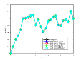
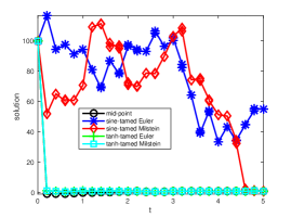
Figure 1: Solution paths from the midpoint scheme (5.2) and tamed schemes (1.5) and (1.6). The time step size $h$ is $10^{-3}$. Left: initial value $X(0)=0$. Right: initial value $X(0)=100$.

In summary, we conclude from this example that tamed schemes can preserve the convergence orders (half-order and first-order). Though the tamed schemes are convergent, requirements on time step sizes are different. Numerical results show that schemes with the hyperbolic tangent function allows larger time steps than those with the sine tame function.

References

- [1] J. Bi, Z. Zhang, A numerical scheme for nonlinear SDEs with both one-sided Lipschitz and Hölder continuous coefficients, In preparation.
- [2] Ĭ. Ī. Gīhman, A. V. Skorohod, Stochastic differential equations, Springer-Verlag, New York, 1972.
- [3] D. J. Higham, X. Mao, A. M. Stuart, Strong convergence of Euler-type methods for nonlinear stochastic differential equations, SIAM J. Numer. Anal. 40 (3) (2002) 1041–1063.
- [4] Y. Hu, Semi-implicit Euler-Maruyama scheme for stiff stochastic equations, in: Stochastic analysis and related topics, Birkhäuser Boston, Boston, MA, 1996, pp. 183–202.
- [5] M. Hutzenthaler, A. Jentzen, On a perturbation theory and on strong convergence rates for stochastic ordinary and partial differential equations with non-globally monotone coefficients, ArXiv, 2014.
- [6] M. Hutzenthaler, A. Jentzen, Numerical approximation of stochastic differential equations with non-globally Lipschitz continuous coefficients, Mem. Amer. Math. Soc. 236 (1112) (2015) 1.
- [7] M. Hutzenthaler, A. Jentzen, P. E. Kloeden, Strong and weak divergence in finite time of Euler’s method for stochastic differential equations with non-globally Lipschitz continuous coefficients, Proc. R. Soc. A (2130) (2011) 1563–1576.
- [8] M. Hutzenthaler, A. Jentzen, P. E. Kloeden, Strong convergence of an explicit numerical method for SDEs with nonglobally Lipschitz continuous coefficients, Ann. Appl. Probab. 22 (4) (2012) 1611–1641.
- [9] M. Hutzenthaler, A. Jentzen, X. Wang, Exponential integrability properties of numerical approximation processes for nonlinear stochastic differential equations, ArXiv, 2013
- [10] P. E. Kloeden, E. Platen, Numerical solution of stochastic differential equations, Springer-Verlag, Berlin, 1992.
- [11] W. Liu, X. Mao, Strong convergence of the stopped Euler-Maruyama method for nonlinear stochastic differential equations, Appl. Math. Comput. 223 (0) (2013) 389 – 400.
- [12] X. Mao, The truncated Euler–Maruyama method for stochastic differential equations, J. Comput. Appl. Math. 290 (2015) 370–384.
- [13] X. Mao, L. Szpruch, Strong convergence and stability of implicit numerical methods for stochastic differential equations with non-globally Lipschitz continuous coefficients, J. Comput. Appl. Math. 238 (2013) 14–28.
- [14] X. Mao, L. Szpruch, Strong convergence rates for backward Euler-Maruyama method for non-linear dissipative-type stochastic differential equations with super-linear diffusion coefficients, Stochastics 85 (1) (2013) 144–171.
- [15] G. N. Milstein, Numerical integration of stochastic differential equations, Kluwer Academic Publishers Group, Dordrecht, 1995.
- [16] G. N. Milstein, E. Platen, H. Schurz, Balanced implicit methods for stiff stochastic systems, SIAM J. Numer. Anal. 35 (3) (1998) 1010–1019.
- [17] G. N. Milstein, M. V. Tretyakov, Stochastic numerics for mathematical physics, Springer-Verlag, Berlin, 2004.
- [18] G. N. Milstein, M. V. Tretyakov, Numerical integration of stochastic differential equations with nonglobally Lipschitz coefficients, SIAM J. Numer. Anal. 43 (3) (2005) 1139–1154.
- [19] S. Sabanis, Euler approximations with varying coefficients: the case of superlinearly growing diffusion coefficients, ArXiv, 2013.
- [20] S. Sabanis, A note on tamed Euler approximations, Electron. Commun. Probab. 18 (2013) no. 47, 1–10.
- [21] L. Szpruch, V-stable tamed Euler schemes, ArXiv, 2013.
- [22] D. Talay, Stochastic Hamiltonian systems: exponential convergence to the invariant measure, and discretization by the implicit Euler scheme, Markov Process. Related Fields 8 (2) (2002) 163–198.
- [23] M. V. Tretyakov, Z. Zhang, A fundamental mean-square convergence theorem for SDEs with locally Lipschitz coefficients and its applications, SIAM J. Numer. Anal. 51 (6) (2013) 3135–3162.
- [24] X. Wang, S. Gan, The tamed Milstein method for commutative stochastic differential equations with non-globally Lipschitz continuous coefficients, J. Difference Equ. Appl. 19 (3) (2013) 466–490.
- [25] X. Zong, F. Wu, C. Huang, Convergence and stability of the semi-tamed Euler scheme for stochastic differential equations with non-Lipschitz continuous coefficients, Appl. Math. Comput. 228 (0) (2014) 240–250.