$Q^{2}$-evolution of parton densities at small $x$ values
and H1 and ZEUS experimental data.

Abstract

It is shown that in the leading twist approximation of the Wilson operator product expansion with “frozen” and analytic strong coupling constants, considering the Bessel-inspired behavior of the structure functions $F_{2}$ and the derivative $\partial\ln F_{2}/\partial\ln(1/x)$ at small $x$ values, obtained for a flat initial condition in the DGLAP evolution equations, leads to a good agreement with the deep inelastic scattering H1 and ZEUS experimental data from HERA.

1 Introduction

A reasonable agreement between HERA data H197 -DIS02 and the next-to-leading-order (NLO) approximation of perturbative Quantum Chromodynamics (QCD) has been observed for $Q^{2}\geq 2$ GeV² (see reviews in CoDeRo and references therein), which gives us a reason to believe that perturbative QCD is capable of describing the evolution of the structure function (SF) $F_{2}$ and its derivatives down to very low $Q^{2}$ values, where all the strong interactions are conventionally considered to be soft processes.

A standard way to study the $x$ behavior of quarks and gluons is to compare the data with the numerical solution to the Dokshitzer-Gribov-Lipatov-Altarelli-Parisi (DGLAP) equations DGLAP by fitting the parameters of $x$-profile of partons at some initial $Q_{0}^{2}$ and the QCD energy scale $\Lambda$ Martin:2009bu ; Ourfits . However, for the purpose of analyzing exclusively the small-$x$ region, there is an alternative to carry out a simpler analysis by using some of the existing analytical solutions to DGLAP equations in the small-$x$ limit BF1 –HT .

To improve the analysis at low $Q^{2}$ values, it is important to consider the well-known infrared modifications of the strong coupling constant. We will use its “frozen” and analytic versions (see, Kotikov:2010bm ; Cvetic:2009kw and references therein).

2 Generalized doubled asymptotic scaling approach

At low-$x$ values there is the simple analytical solution of DGLAP evolution BF1 : the HERA small-$x$ data can be interpreted in terms of the so-called doubled asymptotic scaling (DAS) phenomenon related to the asymptotic behavior of the DGLAP evolution discovered many years ago Rujula .

The original study of BF1 was extended in Munich ; Q2evo ; HT to include the finite parts of anomalous dimensions of Wilson operators . This has led to predictions Q2evo ; HT of the small-$x$ asymptotic form of parton distribution functions (PDFs) in the framework of the DGLAP dynamics starting at some $Q^{2}_{0}$ with the flat function

$$f_{a}(Q^{2}_{0})~{}=~{}A_{a}~{}~{}~{}~{}(\mbox{hereafter }a=q,g),$$ (1)

where $f_{a}$ are the parton distributions multiplied by $x$ and $A_{a}$ are unknown parameters to be determined from the data.

We refer to the approach of Munich ; Q2evo ; HT as generalized DAS approximation. In that approach the flat initial conditions in Eq. (1) determine the basic role of the singular parts of anomalous dimensions, as in the standard DAS case, while the contribution from finite parts of anomalous dimensions and from Wilson coefficients can be considered as corrections which are, however, important for better agreement with experimental data. In the present paper, similary to BF1 –HT , we neglect the contribution from the non-singlet quark component.

The flat initial condition (1) corresponds to the case when parton density tend to some constant value at $x\to 0$ and at some initial value $Q^{2}_{0}$. The main ingredients of the results Q2evo ; HT , are:

• Both, the gluon and quark singlet densities are presented in terms of two components ($"+"$ and $"-"$) which are obtained from the analytic $Q^{2}$-dependent expressions of the corresponding ($"+"$ and $"-"$) PDF moments.

• The twist-two part of the $"-"$ component is constant at small $x$ at any values of $Q^{2}$, whereas the one of the $"+"$ component grows at $Q^{2}\geq Q^{2}_{0}$ as

  $$\sim e^{\sigma},~{}~{}~{}\sigma=2\sqrt{\left[\left|\hat{d}_{+}\right|s-\left(\hat{d}_{++}+\left|\hat{d}_{+}\right|\frac{\beta_{1}}{\beta_{0}}\right)p\right]\ln\left(\frac{1}{x}\right)}\ ,~{}~{}~{}\rho=\frac{\sigma}{2\ln(1/x)}\ ,$$ (2)

  where $\sigma$ and $\rho$ are the generalized Ball–Forte variables,

  $$s=\ln\left(\frac{a_{s}(Q^{2}_{0})}{a_{s}(Q^{2})}\right),~{}~{}p=a_{s}(Q^{2}_{0})-a_{s}(Q^{2}),~{}~{}~{}\hat{d}_{+}=-\frac{12}{\beta_{0}},~{}~{}~{}\hat{d}_{++}=\frac{412}{27\beta_{0}}.$$ (3)

Hereafter we use the notation $a_{s}=\alpha_{s}/(4\pi)$. The first two coefficients of the QCD $\beta$-function in the ${\overline{\mbox{MS}}}$-scheme are $\beta_{0}=11-(2/3)f$ and $\beta_{1}=102-(114/9)f$ with $f$ is being the number of active quark flavors.

Note here that the perturbative coupling constant $a_{s}(Q^{2})$ is different at the leading-order (LO) and NLO approximations. Indeed, from the renormalization group equation we can obtain the following equations for the coupling constant

$$\frac{1}{a_{s}^{\rm LO}(Q^{2})}\,=\,\beta_{0}\ln{\left(\frac{Q^{2}}{\Lambda^{2}_{\rm LO}}\right)},~{}~{}~{}~{}~{}\frac{1}{a_{s}(Q^{2})}\,+\,\frac{\beta_{1}}{\beta_{0}}\ln{\left[\frac{\beta_{0}^{2}a_{s}(Q^{2})}{\beta_{0}+\beta_{1}a_{s}(Q^{2})}\right]}\,=\,\beta_{0}\ln{\left(\frac{Q^{2}}{\Lambda^{2}}\right)}$$ (4)

at the LO and NLO approximations, respoectively. Usually at the NLO level ${\rm\overline{MS}}$-scheme is used, so we apply $\Lambda=\Lambda_{\rm\overline{MS}}$ below.

3 Parton distributions and the structure function $F_{2}$

Here, for simplicity we consider only the LO approximation. The structure function $F_{2}$ and PDFs $f_{a}$ $(a=q,g)$ have the form

$$F_{2}(x,Q^{2}) = e\,f_{q}(x,Q^{2}),~{}~{}f_{a}(x,Q^{2})~{}=~{}f_{a}^{+}(x,Q^{2})+f_{a}^{-}(x,Q^{2}),$$ (5)

where $e=(\sum_{1}^{f}e_{i}^{2})/f$ is an average charge squared.

The small-$x$ asymptotic expressions for parton densities $f^{\pm}_{a}$ look like

$$f^{+}_{g}(x,Q^{2}) = \biggl{(}A_{g}+\frac{4}{9}A_{q}\biggl{)}I_{0}(\sigma)\;e^{-\overline{d}_{+}s}+O(\rho),~{}~{}f^{+}_{q}(x,Q^{2})~{}=~{}\frac{f}{9}\frac{\rho I_{1}(\sigma)}{I_{0}(\sigma)}\,f^{+}_{g}(x,Q^{2})+O(\rho),$$

$$f^{-}_{g}(x,Q^{2}) = -\frac{4}{9}A_{q}e^{-d_{-}s}\,+\,O(x),~{}~{}f^{-}_{q}(x,Q^{2})~{}=~{}A_{q}e^{-d_{-}(1)s}\,+\,O(x),$$ (6)

where $I_{\nu}$ ($\nu=0,1$) are the modified Bessel functions and $\sigma$ and $\rho$ can be found in (2) when $p=0$. The coefficient $\hat{d}_{+}$ (see eq. (3)) and

$$\overline{d}_{+}=1+\frac{20f}{27\beta_{0}},~{}~{}~{}d_{-}=\frac{16f}{27\beta_{0}}$$ (7)

denote singular and regular parts of the anomalous dimensions $d_{+}(n)$ and $d_{-}(n)$, respectively, in the limit $n\to 1$. Here $n$ is a variable in the Mellin space.

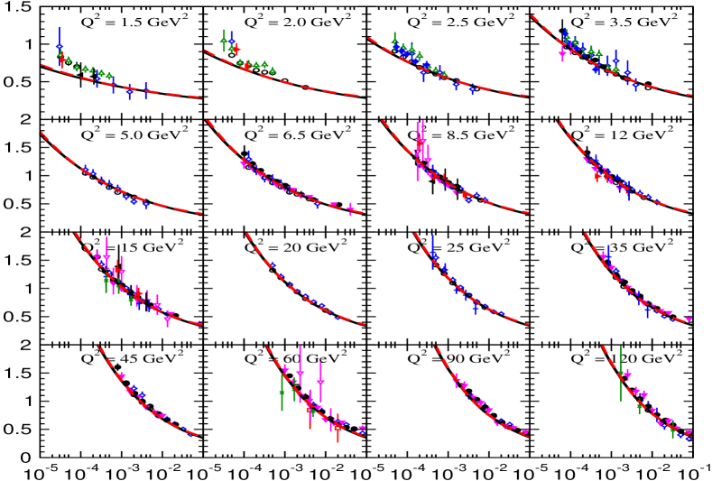
Figure 1: $F_{2}(x,Q^{2})$ as a function of $x$ for different $Q^{2}$ bins. The experimental points are from H1 H197 (open points) and ZEUS ZEUS01 (solid points) at $Q^{2}\geq 1.5$ GeV². The solid curve represents the NLO fit. The dashed curve (hardly distinguishable from the solid one) represents the LO fit.

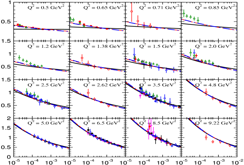
Figure 2: $x$ dependence of $F_{2}(x,Q^{2})$ in bins of $Q^{2}$. The experimental data from H1 (open points) and ZEUS (solid points) are compared with the NLO fits for $Q^{2}\geq 0.5$ GeV² implemented with the canonical (solid lines), frozen (dot-dashed lines), and analytic (dashed lines) versions of the strong-coupling constant. For comparison, also the results obtained in Ref. HT through a fit based on the renormalon model of higher-twist terms are shown (dotted lines).

Table 1: The result of the LO and NLO fits to H1 and ZEUS data for different low $Q^{2}$ cuts. In the fits $f$ is fixed to 4 flavors.

	$A_{g}$	$A_{q}$	$Q_{0}^{2}~{}[{\rm GeV}^{2}]$	$\chi^{2}/n.o.p.$
$Q^{2}\geq 1.5{\rm GeV}^{2}$
LO	0.784$\pm$.016	0.801$\pm$.019	0.304$\pm$.003	754/609
LO$\&$an.	0.932$\pm$.017	0.707$\pm$.020	0.339$\pm$.003	632/609
LO$\&$fr.	1.022$\pm$.018	0.650$\pm$.020	0.356$\pm$.003	547/609
NLO	-0.200$\pm$.011	0.903$\pm$.021	0.495$\pm$.006	798/609
NLO$\&$an.	0.310$\pm$.013	0.640$\pm$.022	0.702$\pm$.008	655/609
NLO$\&$fr.	0.180$\pm$.012	0.780$\pm$.022	0.661$\pm$.007	669/609
$Q^{2}\geq 0.5{\rm GeV}^{2}$
LO	0.641$\pm$.010	0.937$\pm$.012	0.295$\pm$.003	1090/662
LO$\&$an.	0.846$\pm$.010	0.771$\pm$.013	0.328$\pm$.003	803/662
LO$\&$fr.	1.127$\pm$.011	0.534$\pm$.015	0.358$\pm$.003	679/662
NLO	-0.192$\pm$.006	1.087$\pm$.012	0.478$\pm$.006	1229/662
NLO$\&$an.	0.281$\pm$.008	0.634$\pm$.016	0.680$\pm$.007	633/662
NLO$\&$fr.	0.205$\pm$.007	0.650$\pm$.016	0.589$\pm$.006	670/662

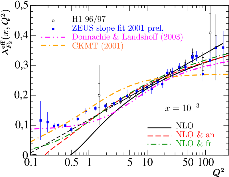
Figure 3: $Q^{2}$ dependence of $\lambda^{\rm eff}_{\rm F_{2}}(x,Q^{2})$ for an average small-$x$ value of $x=10^{-3}$. The experimental data from H1 (open points) and ZEUS (solid points) are compared with the NLO fits for $Q^{2}\geq 0.5$ GeV² implemented with the canonical (solid line), frozen (dot-dashed line), and analytic (dashed line) versions of the strong-coupling constant. The linear rise of $\lambda^{\rm eff}_{\rm F_{2}}(x,Q^{2})$ with $\ln Q^{2}$ is indicated by the straight dashed line. For comparison, also the results obtained in the phenomenological models by Capella et al. CaKaMeTTV (dash-dash-dotted line) and by Donnachie and Landshoff Donnachie:2003cs (dot-dot-dashed line) are shown.

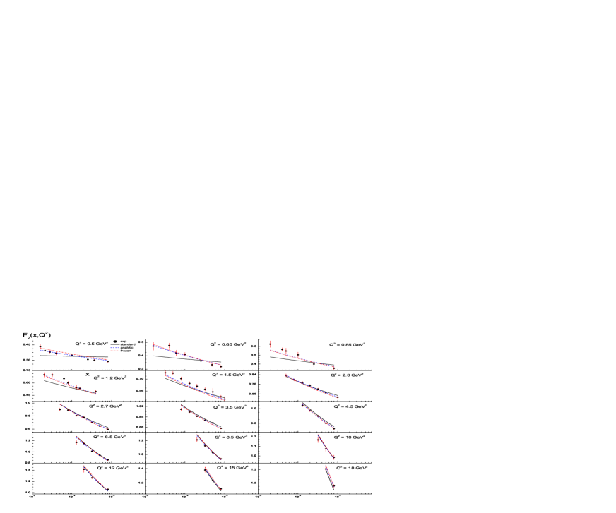
Figure 4: $x$ dependence of $F_{2}(x,Q^{2})$ in bins of $Q^{2}$. The combined experimental data from H1 and ZEUS Collaborations Aaron:2009aa are compared with the NLO fits for $Q^{2}\geq 0.5$ GeV² implemented with the standard (solid lines), frozen (dot-dashed lines), and analytic (dashed lines) versions of the strong coupling constant.

4 Effective slopes

Contrary to the approach in BF1 -HT various groups have been able to fit the available data using a hard input at small $x$: $x^{-\lambda},~{}\lambda>0$ with different $\lambda$ values at low and high $Q^{2}$ (see LoYn -DeJePa ). Such results are well-known at low $Q^{2}$ values DoLa . At large $Q^{2}$ values, for the modern HERA data it is also not very surprising, because improssible to distinguish between the behavior based on a steep input parton parameterization, at quite large $Q^{2}$, and the steep form acquired after the dynamical evolution from a flat initial condition at quite low $Q^{2}$ values.

As it has been mentioned above and shown in Q2evo ; HT ; KoPa02 , the behavior of parton densities and $F_{2}$ given in the Bessel-like form by generalized DAS approach can mimic a power law shape over a limited region of $x$ and $Q^{2}$

$$f_{a}(x,Q^{2})\sim x^{-\lambda^{\rm eff}_{a}(x,Q^{2})}~{}\mbox{ and }~{}F_{2}(x,Q^{2})\sim x^{-\lambda^{\rm eff}_{\rm F_{2}}(x,Q^{2})}.$$

The effective slopes $\lambda^{\rm eff}_{a}(x,Q^{2})$ and $\lambda^{\rm eff}_{\rm F_{2}}(x,Q^{2})$ have the form:

$$\lambda^{\rm eff}_{g}(x,Q^{2})~{}=~{}\frac{f^{+}_{g}(x,Q^{2})}{f_{g}(x,Q^{2})}\,\rho\,\frac{I_{1}(\sigma)}{I_{0}(\sigma)},~{}~{}~{}~{}\lambda^{\rm eff}_{\rm F_{2}}(x,Q^{2})~{}=~{}\lambda^{\rm eff}_{q}(x,Q^{2})~{}=~{}\frac{f^{+}_{q}(x,Q^{2})}{f_{q}(x,Q^{2})}\,\rho\,\frac{I_{2}(\sigma)}{I_{1}(\sigma)}.$$ (8)

The effective slopes $\lambda^{\rm eff}_{a}$ and $\lambda^{\rm eff}_{\rm F_{2}}$ depend on the magnitudes $A_{a}$ of the initial PDFs and also on the chosen input values of $Q^{2}_{0}$ and $\Lambda$. To compare with the experimental data it is necessary the exact expressions (8), but for qualitative analysis it is better to use an approximation. At quite large values of $Q^{2}$, where the “$-$” component is negligible, the dependence on the initial PDFs disappears, having in this case for the asymptotic behavior the following expressions:

$$\lambda^{\rm eff,as}_{g}(x,Q^{2})~{}=~{}\rho\,\frac{I_{1}(\sigma)}{I_{0}(\sigma)}\approx\rho-\frac{1}{4\ln{(1/x)}},~{}~{}~{}\lambda^{\rm eff,as}_{\rm F_{2}}(x,Q^{2})~{}=~{}\lambda^{\rm eff,as}_{q}(x,Q^{2})~{}=~{}\rho\frac{I_{2}(\sigma)}{I_{1}(\sigma)}\approx\rho-\frac{3}{4\ln{(1/x)}}$$ (9)

where the symbol $\approx$ marks the approximation obtained in the expansion of the modified Bessel functions.

5 “Frozen” and analytic coupling constants

In order to improve an agreement at low $Q^{2}$ values, the QCD coupland is modified in the infrared region. We considered Cvetic:2009kw two modifications that effectively increase the argument of the coupling constant at low $Q^{2}$ values (see DoShi ).

In the first case, which is more phenomenological, we introduce freezing of the coupling constant by changing its argument $Q^{2}\to Q^{2}+M^{2}_{\rho}$, where $M_{\rho}$ is the $\rho$-meson mass (see Greco ). Thus, in the above formulae we have to carry out the following replacement:

$$a_{s}(Q^{2})\to a_{\rm fr}(Q^{2})\equiv a_{s}(Q^{2}+M^{2}_{\rho})$$ (10)

The second possibility follows the Shirkov–Solovtsov idea ShiSo concerning the analyticity of the coupling constant that leads to additional power dependence of the latter. Then, in the above formulae the coupling constant $a_{s}(Q^{2})$ should be replaced as follows:

$$a^{\rm LO}_{\rm an}(Q^{2})\,=\,a^{\rm LO}_{s}(Q^{2})-\frac{1}{\beta_{0}}\frac{\Lambda^{2}_{\rm LO}}{Q^{2}-\Lambda^{2}_{\rm LO}},~{}~{}~{}~{}~{}~{}a_{\rm an}(Q^{2})\,=\,a_{s}(Q^{2})-\frac{1}{2\beta_{0}}\frac{\Lambda^{2}}{Q^{2}-\Lambda^{2}}+\ldots\,,$$ (11)

in the LO and NLO approximations, respectively. Here the the symbol $\ldots$ stands for the terms that provide negligible contributions when $Q^{2}\geq 1$ GeV ShiSo . Note that the perturbative coupling constant $a_{s}(Q^{2})$ is different in the LO and NLO approximations (see eq. (4) above).

6 Comparison with experimental data

Using the results of previous section we have analyzed Q2evo ; HT ; Cvetic:2009kw HERA data for $F_{2}$ and the slope $\partial\ln F_{2}/\partial\ln(1/x)$ at small $x$ from the H1 and ZEUS Collaborations H197 -DIS02 . In order to keep the analysis as simple as possible, we fix $f=4$ and $\alpha_{s}(M^{2}_{Z})=0.1166$ (i.e., $\Lambda^{(4)}=284$ MeV) in agreement with the more recent ZEUS results ZEUS01 .

As it is possible to see in Fig. 1 (see also Q2evo ; HT ), the twist-two approximation is reasonable at $Q^{2}\geq 2$ GeV². Moreover, the results of fits in HT have an important property: they are very similar in LO and NLO approximations of perturbation theory. The similarity is related to the fact that the small-$x$ asymptotics of the NLO corrections are usually large and negative (see, for example, $\alpha_{s}$-corrections FaLi ; KoLi to Balitsky–Fadin–Kuraev–Lipatov (BFKL) kernel BFKL ). Then, the LO form $\sim\alpha_{s}(Q^{2})$ for some observable and the NLO one $\sim\alpha_{s}(Q^{2})(1-K\alpha_{s}(Q^{2}))$ with a large value of $K$ are similar, because $\Lambda\gg\Lambda_{\rm LO}$ and, thus, $\alpha_{s}(Q^{2})$ at LO is considerably smaller then $\alpha_{s}(Q^{2})$ at NLO for HERA $Q^{2}$ values.

In other words, performing some resummation procedure (such as Grunberg’s effective-charge method Grunberg ), one can see that the results up to NLO approximation may be represented as $\sim\alpha_{s}(Q^{2}_{\rm eff})$, where $Q^{2}_{\rm eff}\gg Q^{2}$. Indeed, from different studies DoShi ; bfklp ; Andersson , it is well known that at small-$x$ values the effective argument of the coupling constant is higher then $Q^{2}$.

At smaller $Q^{2}$, some modification of the twist-two approximation should be considered. In Ref. HT we have added the higher twist corrections. For renormalon model of higher twists, we have found a good agreement with experimental data at essentially lower $Q^{2}$ values: $Q^{2}\geq 0.5$ GeV² (see Figs. 2 and 3 in HT ), but we have added 4 additional parameters: amplitudes of twist-4 and twist-6 corrections to quark and gluon densities.

To improve the agreement at small $Q^{2}$ values without additional parameters, we modified Cvetic:2009kw the QCD coupling constant. We considered two modifications: analytic and frozen coupling constants, which effectively increase the argument of the coupling constant at small $Q^{2}$ values (in agreement with DoShi ; bfklp ; Andersson ).

Figure 2 and Table 1 show a strong improvement of the agreement with experimental data for $F_{2}$ (almost 2 times!). Similar results can be seen also in Fig. 3 for the experimental data for $\lambda_{F_{2}}^{\rm eff}(x,Q^{2})$ at $x\sim 10^{-3}$, which represents an average of the $x$-values of HERA experimental data. Note that the “frozen” and analytic coupling constants $\alpha_{\rm fr}(Q^{2})$ and $\alpha_{\rm an}(Q^{2})$, lead to very close results (see also KoLiZo ; Kotikov:2010bm ).

Indeed, the fits for $F_{2}(x,Q^{2})$ in HT yielded $Q^{2}_{0}\approx 0.5$–$0.8$ GeV². So, initially we had $\lambda^{\rm eff}_{F_{2}}(x,Q^{2}_{0})=0$, as suggested by Eq. (1). The replacements of Eqs. (10) and (11) modify the value of $\lambda^{\rm eff}_{F_{2}}(x,Q^{2}_{0})$. For the “frozen” and analytic coupling constants $\alpha_{\rm fr}(Q^{2})$ and $\alpha_{\rm an}(Q^{2})$, the value of $\lambda^{\rm eff}_{F_{2}}(x,Q^{2}_{0})$ is nonzero and the slopes are quite close to the experimental data at $Q^{2}\approx 0.5$ GeV². Nevertheless, for $Q^{2}\leq 0.5$ GeV², there is still some disagreement with the data for the slope $\lambda^{\rm eff}_{F_{2}}(x,Q^{2})$, which needs additional investigation. Note that at $Q^{2}\geq 0.5$ GeV² our results for $\lambda^{\rm eff}_{F_{2}}(x,Q^{2})$ are even better the results of phenomenological models CaKaMeTTV ; Donnachie:2003cs .

Table 2: The results of LO and NLO fits to H1 $\&$ ZEUS data Aaron:2009aa , with various lower cuts on $Q^{2}$; in the fits the number of flavors $f$ is fixed to 4.

	$A_{g}$	$A_{q}$	$Q_{0}^{2}~{}[{\rm GeV}^{2}]$	$\chi^{2}/n.d.f.$
$Q^{2}\geq 5{\rm GeV}^{2}$
LO	0.623$\pm$0.055	1.204$\pm$0.093	0.437$\pm$0.022	1.00
LO$\&$an.	0.796$\pm$0.059	1.103$\pm$0.095	0.494$\pm$0.024	0.85
LO$\&$fr.	0.782$\pm$0.058	1.110$\pm$0.094	0.485$\pm$0.024	0.82
NLO	-0.252$\pm$0.041	1.335$\pm$0.100	0.700$\pm$0.044	1.05
NLO$\&$an.	0.102$\pm$0.046	1.029$\pm$0.106	1.017$\pm$0.060	0.74
NLO$\&$fr.	-0.132$\pm$0.043	1.219$\pm$0.102	0.793$\pm$0.049	0.86
$Q^{2}\geq 3.5{\rm GeV}^{2}$
LO	0.542$\pm$0.028	1.089$\pm$0.055	0.369$\pm$0.011	1.73
LO$\&$an.	0.758$\pm$0.031	0.962$\pm$0.056	0.433$\pm$0.013	1.32
LO$\&$fr.	0.775$\pm$0.031	0.950$\pm$0.056	0.432$\pm$0.013	1.23
NLO	-0.310$\pm$0.021	1.246$\pm$0.058	0.556$\pm$0.023	1.82
NLO$\&$an.	0.116$\pm$0.024	0.867$\pm$0.064	0.909$\pm$0.330	1.04
NLO$\&$fr.	-0.135$\pm$0.022	1.067$\pm$0.061	0.678$\pm$0.026	1.27
$Q^{2}\geq 2.5{\rm GeV}^{2}$
LO	0.526$\pm$0.023	1.049$\pm$0.045	0.352$\pm$0.009	1.87
LO$\&$an.	0.761$\pm$0.025	0.919$\pm$0.046	0.422$\pm$0.010	1.38
LO$\&$fr.	0.794$\pm$0.025	0.900$\pm$0.047	0.425$\pm$0.010	1.30
NLO	-0.322$\pm$0.017	1.212$\pm$0.048	0.517$\pm$0.018	2.00
NLO$\&$an.	0.132$\pm$0.020	0.825$\pm$0.053	0.898$\pm$0.026	1.09
NLO$\&$fr.	-0.123$\pm$0.018	1.016$\pm$0.051	0.658$\pm$0.021	1.31
$Q^{2}\geq 0.5{\rm GeV}^{2}$
LO	0.366$\pm$0.011	1.052$\pm$0.016	0.295$\pm$0.005	5.74
LO$\&$an.	0.665$\pm$0.012	0.804$\pm$0.019	0.356$\pm$0.006	3.13
LO$\&$fr.	0.874$\pm$0.012	0.575$\pm$0.021	0.368$\pm$0.006	2.96
NLO	-0.443$\pm$0.008	1.260$\pm$0.012	0.387$\pm$0.010	6.62
NLO$\&$an.	0.121$\pm$0.008	0.656$\pm$0.024	0.764$\pm$0.015	1.84
NLO$\&$fr.	-0.071$\pm$0.007	0.712$\pm$0.023	0.529$\pm$0.011	2.79

At the next step we considered Kotikov:2012sm the combined H1$\&$ZEUS data for $F_{2}$ Aaron:2009aa . As can be seen from Fig. 4 and Table 2, the twist-two approximation is reasonable for $Q^{2}\geq 2$ GeV². At lower $Q^{2}$ we observe that the fits in the cases with “frozen” and analytic strong coupling constants are very similar (see also KoLiZo ; Cvetic:2009kw ; Kotikov:2010bm ) and describe the data in the low $Q^{2}$ region significantly better than the standard fit. Nevertheless, for $Q^{2}\leq 1.5$ GeV² there is still some disagreement with the data, which needs to be additionally studied. In particular, the BFKL resummation BFKL may be important here Kowalski:2012ur . It can be added in the generalized DAS approach according to the discussion in Ref. KoBaldin .

7 Conclusions

We have shown the $Q^{2}$-dependence of the structure functions $F_{2}$ and the slope $\lambda^{\rm eff}_{F_{2}}=\partial\ln F_{2}/\partial\ln(1/x)$ at small-$x$ values in the framework of perturbative QCD. Our twist-two results are in a very good agreement with precise HERA data for $Q^{2}\geq 2$ GeV², where perturbative theory is applicable. Using the “frozen” and analytic coupling constants $\alpha_{\rm fr}(Q^{2})$ and $\alpha_{\rm an}(Q^{2})$ improves an agreement with the recent HERA data Surrow ; H1slo ; DIS02 for the slope $\lambda^{\rm eff}_{F_{2}}(x,Q^{2})$ for small $Q^{2}$ values, $Q^{2}\geq 0.5$ GeV².

As the next spep, we are going to adopt the Grunberg approach Grunberg together with the “frozen” and analytic modifications of the strong coupling constant for analyse of the combined H1$\&$ZEUS data for $F_{2}$ Aaron:2009aa . The similar study has been done recently Kotikov:2012eq for experimental data of the Bjorken sum rule.

References

- (1) H1 Collab. (C. Adloff et al.), Nucl. Phys. B 497 (1997) 3; Eur. Phys. J. C 21 (2001) 33.
- (2) ZEUS Collab. (S. Chekanov et al.), Eur. Phys. J. C 21 (2001) 443.
- (3) H1 and ZEUS Collab. ( F. D. Aaron et al.), JHEP 1001 (2010) 109.
- (4) H1 and ZEUS Collab. (B. Surrow), Phenomenological studies of inclusive e p scattering at low momentum transfer Q**2, hep-ph/0201025.
- (5) H1 Collab. (C. Adloff et al.), Phys. Lett. B 520 (2001) 183.
- (6) H1 Collab. (T. Lastovicka), Acta Phys. Polon. B 33 (2002) 2835; H1 Collab. (J. Gayler), Acta Phys. Polon. B 33 (2002) 2841.
- (7) A. M. Cooper-Sarkar, R. C. E. Devenish, and A. De Roeck, Int. J. Mod. Phys. A 13 (1998) 3385; A. V. Kotikov, Phys. Part. Nucl. 38 (2007) 1. [Erratum-ibid. 38 (2007) 828].
- (8) V. N. Gribov and L. N. Lipatov, Sov. J. Nucl. Phys. 15 (1972) 438, 675; L. N. Lipatov, Sov. J. Nucl. Phys. 20 (1975) 94; G. Altarelli and G. Parisi, Nucl. Phys. B 126 (1977) 298; Yu. L. Dokshitzer, Sov. Phys. JETP 46 (1977) 641.
- (9) A. D. Martin, W. J. Stirling, R. S. Thorne and G. Watt, Eur. Phys. J. C 64 (2009) 653; H. -L. Lai, J. Huston, Z. Li, P. Nadolsky, J. Pumplin, D. Stump and C. -P. Yuan, Phys. Rev. D 82 (2010) 054021; S. Alekhin, J. Blumlein and S. Moch, Phys. Rev. D 86 (2012) 054009; R. D. Ball, V. Bertone, S. Carrazza, C. S. Deans, L. Del Debbio, S. Forte, A. Guffanti and N. P. Hartland et al., Nucl. Phys. B 867 (2013) 244; P. Jimenez-Delgado and E. Reya, Phys. Rev. D 80 (2009) 114011; Phys. Rev. D 79 (2009) 074023
- (10) A. V. Kotikov, G. Parente, and J. Sanchez Guillen, Z. Phys. C 58 (1993) 465; G. Parente, A. V. Kotikov, and V. G. Krivokhizhin, Phys. Lett. B 333 (1994) 190; A. L. Kataev, A. V. Kotikov, G. Parente, and A. V. Sidorov, Phys. Lett. B 388 (1996) 179; Phys. Lett. B 417 (1998) 374; A. L. Kataev, G. Parente, and A. V. Sidorov, Nucl. Phys. B 573 (2000) 405; A. V. Kotikov and V. G. Krivokhijine, Phys. At. Nucl. 68 (2005) 1873; B. G. Shaikhatdenov, A. V. Kotikov, V. G. Krivokhizhin and G. Parente, Phys. Rev. D 81 (2010) 034008 [Erratum-ibid. D 81 (2010) 079904].
- (11) R. D. Ball and S. Forte, Phys. Lett. B 336 (1994) 77.
- (12) L. Mankiewicz, A. Saalfeld, and T. Weigl, Phys. Lett. B 393 (1997) 175.
- (13) A. V. Kotikov and G. Parente, Nucl. Phys. B 549 (1999) 242; Nucl. Phys. (Proc. Suppl.) A 99 (2001) 196. [hep-ph/0010352].
- (14) A. Yu. Illarionov, A. V. Kotikov, and G. Parente, Phys. Part. Nucl. 39 (2008) 307; Nucl. Phys. (Proc. Suppl.) 146 (2005) 234.
- (15) A. V. Kotikov, V. G. Krivokhizhin and B. G. Shaikhatdenov, Phys. Atom. Nucl. 75 (2012) 507.
- (16) G. Cvetic, A. Y. .Illarionov, B. A. Kniehl and A. V. Kotikov, Phys. Lett. B 679 (2009) 350.
- (17) A. De Rújula, S. L. Glashow, H. D. Politzer, S.B. Treiman, F. Wilczek, and A. Zee, Phys. Rev. D 10, 1649 (1974) 1649.
- (18) S. Albino, P. Bolzoni, B. A. Kniehl and A. Kotikov, Nucl. Phys. B 851 (2011) 86; Nucl. Phys. B 855 (2012) 801.
- (19) P. Bolzoni, B. A. Kniehl and A. V. Kotikov, Phys. Rev. Lett. 109 (2012) 242002; Nucl. Phys. B 875 (2013) 18.
- (20) C. Lopez and F. J. Ynduráin, Nucl. Phys. B 171 (1980) 231; Nucl. Phys. B 183 (1981) 157; C. Lopez, F. Barreiro, and F. J. Ynduráin, Z. Phys. C 72 (1996) 561; K. Adel, F. Barreiro, and F. J. Ynduráin, Nucl. Phys. B 495 (1997) 221.
- (21) A. Donnachie and P. V. Landshoff, Phys. Lett. B 296 (1992) 227; 437 (1998) 408.
- (22) H. Abramowitz, E. M. Levin, A. Levy, and U. Maor, Phys. Lett. B 269 (1991) 465; A. V. Kotikov, Mod. Phys. Lett. A 11 (1996) 103; Phys. At. Nucl. 59 (1996) 2137.
- (23) A. V. Kotikov, Phys. At. Nucl. 56 (1993) 1276; Phys. Rev. D 49 (1994) 5746.
- (24) G. M. Frichter, D. W. McKay, and J. P. Ralston, Phys. Rev. Lett. 74 (1995) 1508.
- (25) A. Capella, A. B. Kaidalov, C. Merino, and J. Tran Thanh Van, Phys. Lett. B 337 (1994) 358; A. B. Kaidalov, C. Merino, and D. Pertermann, Eur. Phys. J. C 20 (2001) 301.
- (26) P. Desgrolard, L. L. Jenkovszky, and F. Paccanoni, Eur. Phys. J. C 7 (1999) 655; V. I. Vovk, A. V. Kotikov, and S. I. Maximov, Theor. Math. Phys. 84 (1990) 744; L. L. Jenkovszky, A. V. Kotikov, and F. Paccanoni, Sov. J. Nucl. Phys. 55 (1992) 1224; JETP Lett. 58 (1993) 163; Phys. Lett. B 314 (1993) 421; A. V. Kotikov, S. I. Maximov, and I. S. Parobij, Theor. Math. Phys. 111 (1997) 442.
- (27) A. V. Kotikov and G. Parente, J. Exp. Theor. Phys. 97 (2003) 859.
- (28) G. Curci, M. Greco, and Y. Srivastava, Phys. Rev. Lett. 43 (1979) 834; Nucl. Phys. B 159 (1979) 451; M. Greco, G. Penso, and Y. Srivastava, Phys. Rev. D 21 (1980) 2520; PLUTO Collab. (C. Berger et al.), Phys. Lett. B 100 (1981) 351; N. N. Nikolaev and B. M. Zakharov, Z. Phys. C 49 (1991) 607; 53 (1992) 331; B. Badelek, J. Kwiecinski, and A. Stasto, Z. Phys. C 74 (1997) 297.
- (29) D. V. Shirkov and I. L. Solovtsov, Phys. Rev. Lett 79 (1997) 1209; Theor. Math. Phys. 120 (1999) 1220.
- (30) V. S. Fadin and L. N. Lipatov, Phys. Lett. B 429 (1998) 127; G. Camici and M. Ciafaloni, Phys. Lett. B430 (1998) 349.
- (31) A. V. Kotikov and L. N. Lipatov, Nucl. Phys. B 582 (2000) 19; Nucl. Phys. B 661 (2003) 19.
- (32) L. N. Lipatov, Sov. J. Nucl. Phys. 23 (1976) 338; E. A. Kuraev, L. N. Lipatov, and V. S. Fadin, Phys. Lett. B 60 (1975) 50; Sov. Phys. JETP 44 (1976) 443; 45 (1977) 199; Ya. Ya. Balitzki and L. N. Lipatov, Sov. J. Nucl. Phys. 28 (1978) 822; L. N. Lipatov, Sov. Phys. JETP 63 (1986) 904.
- (33) G. Grunberg, Phys. Rev. D 29 (1984) 2315; Phys. Lett. B 95 (1980) 70.
- (34) Yu. L. Dokshitzer and D. V. Shirkov, Z. Phys. C 67 (1995) 449; A. V. Kotikov, JETP Lett. 59 (1994) 1; Phys. Lett. B 338 (1994) 349; W. K. Wong, Phys. Rev. D 54 (1996) 1094.
- (35) S. J. Brodsky, V. S. Fadin, V. T. Kim, L.N. Lipatov, G.B. Pivovarov, JETP. Lett. 70 (1999) 155; M. Ciafaloni, D. Colferai, and G. P. Salam, Phys. Rev. D 60 (1999) 114036 ; JHEP 07 (2000) 054; R. S. Thorne, Phys. Lett. B 474 (2000) 372; Phys. Rev. D 60 (1999) 054031; 64 (2001) 074005; G. Altarelli, R. D. Ball, and S. Forte, Nucl. Phys. B 621 (2002) 359.
- (36) Bo Andersson et al., Eur. Phys. J. C 25 (2002) 77.
- (37) A. V. Kotikov, A. V. Lipatov, and N. P. Zotov, J. Exp. Theor. Phys. 101 (2005) 811.
- (38) A. Donnachie and P. V. Landshoff, Acta Phys. Polon. B 34 (2003) 2989.
- (39) A. V. Kotikov and B. G. Shaikhatdenov, Phys. Part. Nucl. 44 (2013) 543.
- (40) H. Kowalski, L. N. Lipatov and D. A. Ross, Phys. Part. Nucl. 44 (2013) 547.
- (41) A. V. Kotikov, PoS Baldin-ISHEPP-XXI (2012) 033 [ arXiv:1212.3733 [hep-ph]].
- (42) A. V. Kotikov and B. G. Shaikhatdenov, Phys. Part. Nucl. 45 (2014) 26.