Zonal flow scaling in rapidly-rotating compressible convection

Abstract

The surface winds of Jupiter and Saturn are primarily zonal. Each planet exhibits strong prograde equatorial flow flanked by multiple alternating zonal winds at higher latitudes. The depth to which these flows penetrate has long been debated and is still an unsolved problem. Previous rotating convection models that obtained multiple high latitude zonal jets comparable to those on the giant planets assumed an incompressible (Boussinesq) fluid, which is unrealistic for gas giant planets. Later models of compressible rotating convection obtained only few high latitude jets which were not amenable to scaling analysis.

Here we present 3-D numerical simulations of compressible convection in rapidly-rotating spherical shells. To explore the formation and scaling of high-latitude zonal jets, we consider models with a strong radial density variation and a range of Ekman numbers, while maintaining a zonal flow Rossby number characteristic of Saturn.

All of our simulations show a strong prograde equatorial jet outside the tangent cylinder. At low Ekman numbers several alternating jets form in each hemisphere inside the tangent cylinder. To analyse jet scaling of our numerical models and of Jupiter and Saturn, we extend Rhines scaling based on a topographic $\beta$-parameter, which was previously applied to an incompressible fluid in a spherical shell, to compressible fluids. The jet-widths predicted by this modified Rhines length are found to be in relatively good agreement with our numerical model results and with cloud tracking observations of Jupiter and Saturn.

1 Introduction

The surface flows of the gas giants Jupiter and Saturn are dominated by strong zonal motions (i.e. azimuthal flows). Zonal wind profiles at the surface are obtained by tracking cloud features with ground-based and space observations (e.g. Sanchez-Lavega et al., 2000; Porco et al., 2003, 2005; Vasavada and Showman, 2005).

As shown in Fig. 1, these zonal winds form a differential rotation profile with alternating eastward and westward flows. Both gas giants feature a strong prograde equatorial jet flanked by several weaker alternating secondary jets. Jupiter’s central equatorial jet reaches a maximum velocity around 100-140 m/s and covers latitudes within $\pm 15^{\circ}$. However the region of fast equatorial zonal flow extends to roughly $\pm 25^{\circ}$, and features several strong prograde and retrograde jets that display marked equatorial asymmetry. The secondary undulating zonal winds at higher latitudes are weaker ($\sim 10-20$ m/s) and narrower than the equatorial flow. Saturn’s equatorial flow is stronger than that of Jupiter, wider, and more symmetrical, with a single equatorial jet extending roughly $\pm 30^{\circ}$ in latitude. It is flanked by several secondary jets in each hemisphere. These winds are significantly shifted towards the prograde direction when assuming the rotation period measured by Voyager (Desch and Kaiser, 1981). However, the suitability of this so-called System III rotation period, which is based on Saturn’s kilometric radio (SKR) emissions, for characterizing the mean planetary rotation rate has been questioned. The current Cassini space mission has measured an apparent 6 minute increase in the SKR rotation period since Voyager (e.g. Sánchez-Lavega, 2005). This simple change of 1% in the rotation rate can substantially modify the zonal wind speed (typically around 20% near the equator). Since such changes in the planetary rotation rate are unlikely (Heimpel and Aurnou, 2012), alternative rotation systems have been proposed. Here we adopt the System IIIw rotation period of Read et al. (2009), which is based on an analysis of potential vorticity. This System IIIw rotation period yields more symmetric zonal flows between the prograde and the retrograde directions (see Fig. 1). The amplitude of the equatorial flow then reduces from 450 m/s in the System III rotation period to 370 m/s in System IIIw.

Figure 1: Surface zonal flow profiles for Jupiter (left panel) and Saturn (right panel). Jupiter’s zonal flow profiles come from Cassini’s data by Porco et al. (2003) and Vasavada and Showman (2005). Saturn’s profiles in the two rotations systems have been derived by Read et al. (2009). The conversion between zonal winds velocities in m/s and Rossby numbers is given by $u/\Omega r_{o}$, $r_{o}$ being the planetary radius at the $1$ bar level.

Modelling of zonal wind dynamics can be categorised in two main approaches. In “shallow models”, which are typically based on the hydrostatic approximation of fluid dynamics, the dynamics is confined to a very thin layer close to the cloud level (e.g. Vallis, 2006; Liu and Schneider, 2011). In this approach, zonal winds are maintained by turbulent motions coming from several possible physical forcings that occur at the stably-stratified cloud level (e.g. latent heat release or solar radiation). These shallow models reproduce several features observed on Jupiter and Saturn and notably the alternating direction of the zonal winds (Williams, 1978; Cho and Polvani, 1996). While earlier models yielded a retrograde equatorial jet for both gas giants, prograde equatorial flow has been obtained in more recent models via the inclusion of additional forcing mechanisms, such as water vapor condensation (Lian and Showman, 2010) or enhanced radiative damping (e.g. Liu and Schneider, 2011).

In an alternative approach, zonal winds may be driven by deep-seated convection. This is supported by the latitudinal thermal emission profiles of Jupiter and Saturn, which are relatively flat, implying that deep-seated, outward directed heat flow exceeds absorbed solar heat for both planets (Ingersoll, 1976; Pirraglia, 1984). Although deep convection must drive the dynamos that produce the global magnetic fields of Jupiter and Saturn, it is thought that fast zonal flows would be strongly attenuated at depth by the magnetic braking resulting from the strong increase in the electrical conductivity (Guillot et al., 2004; French et al., 2012). Based on an estimate of the associated Ohmic dissipation, Liu et al. (2008) concluded that the zonal flows must therefore be confined to a relatively thin layer (i.e. $0.96\,R_{J}$ and $0.85\,R_{S}$). This magnetic exclusion of fast zonal flow to an outer region has been demonstrated in recent dynamo models that include radially variable electrical conductivity (Heimpel and Gómez Pérez, 2011; Duarte et al., 2013).

The deep convection hypothesis has been tested by 3-D numerical models of turbulent convection in rapidly-rotating spherical shells (e.g. Christensen, 2001; Heimpel et al., 2005). Rapid rotation causes convection to develop as axially-oriented quasi-geostrophic columns (Busse, 1970). This columnar flow gives rise to Reynolds stresses, a statistical correlation between the convective flow components that feeds energy into zonal flows (e.g. Busse, 1994). The usual prograde tilt of the convective columns goes along with a positive flux of angular momentum away from the rotation axis that yields an eastward equatorial flow (e.g. Zhang, 1992). While such models can easily reproduce the correct direction and amplitude of the equatorial jets observed on Jupiter and Saturn, they usually fail to produce multiple high-latitude jets (Christensen, 2002). Numerical models in relatively deep layers and moderately small Ekman numbers (i.e. aspect ratio $r_{i}/r_{o}=0.6$ and $E=10^{-4}-10^{-5}$) typically produce only a pair of jets in each hemisphere (Christensen, 2001; Jones and Kuzanyan, 2009; Gastine and Wicht, 2012).

Reaching quasi-geostrophic turbulence in a 3-D model of rotating convection is indeed numerically very demanding. These numerical difficulties can be significantly reduced by using the quasi-geostrophic approximation which includes the effects of the curvature of the spherical shell (i.e. the topographic $\beta$-effect) while solving the flow only in the 2-D equatorial plane (Aubert et al., 2003; Schaeffer and Cardin, 2005). For instance, the two-dimensional annulus model of rotating convection considered by Jones et al. (2003); Rotvig and Jones (2006) and Teed et al. (2012) allows very low Ekman numbers to be reached. Multiple alternating zonal flows have been found and the typical width of each jet scales with the Rhines length (e.g. Rhines, 1975; Danilov and Gurarie, 2002; Read et al., 2004; Sukoriansky et al., 2007). Independently of these models, the 3-D simulations of Heimpel et al. (2005) and Heimpel and Aurnou (2007) were computed with lower Ekman numbers and larger aspect ratio ($r_{i}/r_{o}\geq 0.85$) than previous numerical models (e.g. Christensen, 2001). These simulations show clear evidence of multiple jets inside the tangent cylinder. While these simulations produce fewer bands than observed in the quasi-geostrophic simulations, at least in part due to the unavoidable computational limitations, the width of each zonal band follows the Rhines scaling (Heimpel and Aurnou, 2007, hereafter HA07).

Most of the previous models have employed the Boussinesq approximation where compressibility effects are simply ignored. In giant planets, however, the density increases by more than 1000 in the molecular envelope (Guillot, 1999; French et al., 2012) and the applicability of the topographic Rhines scaling is therefore questionable (Evonuk, 2008). More recent anelastic models that allow to incorporate compressibility effects have nevertheless shown several similarities with the previous Boussinesq studies. While the density contrast affects the small-scale convective motions, the large-scale zonal flows are relatively unaffected by the density stratification (Jones and Kuzanyan, 2009; Gastine and Wicht, 2012). However, these results seem incompatible with the new vorticity source introduced by compressibility, which may change the definition of the $\beta$-effect (e.g. Ingersoll and Pollard, 1982; Glatzmaier et al., 2009; Verhoeven and Stellmach, 2014). As pointed out by Jones and Kuzanyan (2009), defining a consistent Rhines scaling in a compressible fluid is not straightforward.

To tackle this problem, we consider numerical models of rapidly-rotating convection in a compressible fluid. We present numerical simulations of a thin spherical shell ($r_{i}/r_{o}=0.85$) with a strong density stratification ($\rho_{\text{bot}}/\rho_{\text{top}}\simeq 150$). A series of simulations, with decreasing Ekman number, are employed to gradually reach the multiple-jets regime. To analyse the zonal flow scaling, we present a consistent derivation of Rhines scaling in compressible fluids.

The paper is organised as follows. In section 2, we present the anelastic formulation and the numerical method. The results of the numerical simulations are presented in section 3. A new derivation of compressible Rhines scaling is presented in section 4. In section 5, we concentrate on the applications to numerical models and gas giants, before concluding in section 6.

2 Hydrodynamical model

2.1 Governing equations

We consider numerical simulations of a compressible fluid in a spherical shell rotating at a constant rotation rate $\Omega$ about the $z$-axis. Following Christensen and Aubert (2006), we adopt a dimensionless formulation of the Navier-Stokes equations where $\Omega^{-1}$ is the time unit and the spherical shell thickness $d=r_{o}-r_{i}$ is the reference lengthscale. Entropy is given in units of $\Delta s$, the fixed entropy contrast over the layer. Density and temperature are non-dimensionalised using $\rho_{o}=\tilde{\rho}(r=r_{o})$ and $T_{o}=\tilde{T}(r=r_{o})$, their reference values at the outer boundary. Heat capacity $c_{p}$, kinematic viscosity $\nu$ and thermal diffusivity $\kappa$ are assumed to be constant.

We employ the anelastic approximation of Braginsky and Roberts (1995) and Lantz and Fan (1999) which allows to incorporate the effects of density stratification while filtering out fast acoustic waves (see also Brown et al., 2012). This approximation assumes an hydrostatic and adiabatic reference state given by $d\tilde{T}/dr=-g/c_{p}$. Assuming an ideal gas leads to a polytropic equation of state given by $\tilde{\rho}=\tilde{T}^{m}$, $m$ being the polytropic index. Following Jones and Kuzanyan (2009); Gastine and Wicht (2012) and Gastine et al. (2013), we assume that the mass is concentrated in the inner part, such that $g\propto 1/r^{2}$ provides a good first-order approximation of the gravity profile in the molecular envelope of a giant planet. This leads to the following temperature $\tilde{T}$ and density $\tilde{\rho}$ profiles

$$\tilde{T}(r)=\dfrac{c_{0}}{(1-\eta)r}+1-c_{0}\quad\text{and}\quad\tilde{\rho}(r)=\tilde{T}^{m},$$ (1)

where $c_{0}=\eta/(1-\eta)[\exp(N_{\rho}/m)-1]$. $N_{\rho}=\ln\tilde{\rho}(r_{i})/\tilde{\rho}(r_{o})$ is the number of density scale heights of the background density profile and $\eta=r_{i}/r_{o}$ is the aspect ratio of the spherical shell.

The thermodynamic quantities, density, pressure and temperature are then decomposed into the sum of the reference state and small perturbations $\tilde{x}(r)+x^{\prime}(r,\theta,\phi)$. The dimensionless equations that govern compressible convection under the anelastic approximation are given by

$$\mathchoice{\mbox{\boldmath$\displaystyle\nabla$}}{\mbox{\boldmath$\textstyle\nabla$}}{\mbox{\boldmath$\scriptstyle\nabla$}}{\mbox{\boldmath$\scriptscriptstyle\nabla$}}\cdot\left(\tilde{\rho}\mathchoice{\mbox{\boldmath$\displaystyle u$}}{\mbox{\boldmath$\textstyle u$}}{\mbox{\boldmath$\scriptstyle u$}}{\mbox{\boldmath$\scriptscriptstyle u$}}\right)=0,$$ (2)

$$\dfrac{\partial\mathchoice{\mbox{\boldmath$\displaystyle u$}}{\mbox{\boldmath$\textstyle u$}}{\mbox{\boldmath$\scriptstyle u$}}{\mbox{\boldmath$\scriptscriptstyle u$}}}{\partial t}+\mathchoice{\mbox{\boldmath$\displaystyle u$}}{\mbox{\boldmath$\textstyle u$}}{\mbox{\boldmath$\scriptstyle u$}}{\mbox{\boldmath$\scriptscriptstyle u$}}\cdot\mathchoice{\mbox{\boldmath$\displaystyle\nabla$}}{\mbox{\boldmath$\textstyle\nabla$}}{\mbox{\boldmath$\scriptstyle\nabla$}}{\mbox{\boldmath$\scriptscriptstyle\nabla$}}\mathchoice{\mbox{\boldmath$\displaystyle u$}}{\mbox{\boldmath$\textstyle u$}}{\mbox{\boldmath$\scriptstyle u$}}{\mbox{\boldmath$\scriptscriptstyle u$}}+2\mathchoice{\mbox{\boldmath$\displaystyle e_{z}$}}{\mbox{\boldmath$\textstyle e_{z}$}}{\mbox{\boldmath$\scriptstyle e_{z}$}}{\mbox{\boldmath$\scriptscriptstyle e_{z}$}}\times\mathchoice{\mbox{\boldmath$\displaystyle u$}}{\mbox{\boldmath$\textstyle u$}}{\mbox{\boldmath$\scriptstyle u$}}{\mbox{\boldmath$\scriptscriptstyle u$}}=-\mathchoice{\mbox{\boldmath$\displaystyle\nabla$}}{\mbox{\boldmath$\textstyle\nabla$}}{\mbox{\boldmath$\scriptstyle\nabla$}}{\mbox{\boldmath$\scriptscriptstyle\nabla$}}{\dfrac{p}{\tilde{\rho}}}+Ra^{*}\dfrac{r_{o}^{2}}{r^{2}}s\,\mathchoice{\mbox{\boldmath$\displaystyle e_{r}$}}{\mbox{\boldmath$\textstyle e_{r}$}}{\mbox{\boldmath$\scriptstyle e_{r}$}}{\mbox{\boldmath$\scriptscriptstyle e_{r}$}}+\dfrac{E}{\tilde{\rho}}\mathchoice{\mbox{\boldmath$\displaystyle\nabla$}}{\mbox{\boldmath$\textstyle\nabla$}}{\mbox{\boldmath$\scriptstyle\nabla$}}{\mbox{\boldmath$\scriptscriptstyle\nabla$}}\cdot\mathsf{S},$$ (3)

$$\tilde{\rho}\tilde{T}\left(\dfrac{\partial s}{\partial t}+\mathchoice{\mbox{\boldmath$\displaystyle u$}}{\mbox{\boldmath$\textstyle u$}}{\mbox{\boldmath$\scriptstyle u$}}{\mbox{\boldmath$\scriptscriptstyle u$}}\cdot\mathchoice{\mbox{\boldmath$\displaystyle\nabla$}}{\mbox{\boldmath$\textstyle\nabla$}}{\mbox{\boldmath$\scriptstyle\nabla$}}{\mbox{\boldmath$\scriptscriptstyle\nabla$}}s\right)=\dfrac{\text{E}}{\text{Pr}}\mathchoice{\mbox{\boldmath$\displaystyle\nabla$}}{\mbox{\boldmath$\textstyle\nabla$}}{\mbox{\boldmath$\scriptstyle\nabla$}}{\mbox{\boldmath$\scriptscriptstyle\nabla$}}\cdot\left(\tilde{\rho}\tilde{T}\mathchoice{\mbox{\boldmath$\displaystyle\nabla$}}{\mbox{\boldmath$\textstyle\nabla$}}{\mbox{\boldmath$\scriptstyle\nabla$}}{\mbox{\boldmath$\scriptscriptstyle\nabla$}}s\right)+\dfrac{\text{E}}{\text{Ra}^{*}}(1-\eta)c_{o}\,Q_{\nu},$$ (4)

where $\textstyle u$, $p$ and $s$ are velocity, pressure and entropy, respectively. The traceless rate-of-strain tensor $\mathsf{S}$ is given by

$$\mathsf{S}_{ij}=2\tilde{\rho}\left(\mathsf{e}_{ij}-\frac{1}{3}\delta_{ij}\mathchoice{\mbox{\boldmath$\displaystyle\nabla$}}{\mbox{\boldmath$\textstyle\nabla$}}{\mbox{\boldmath$\scriptstyle\nabla$}}{\mbox{\boldmath$\scriptscriptstyle\nabla$}}\cdot\mathchoice{\mbox{\boldmath$\displaystyle u$}}{\mbox{\boldmath$\textstyle u$}}{\mbox{\boldmath$\scriptstyle u$}}{\mbox{\boldmath$\scriptscriptstyle u$}}\right)\quad\text{with}\quad\mathsf{e}_{ij}=\dfrac{1}{2}\left(\frac{\partial u_{i}}{\partial x_{j}}+\frac{\partial u_{j}}{\partial x_{i}}\right),$$ (5)

where $\delta_{ij}$ is the identity matrix. $Q_{\nu}$ is the viscous heating contribution expressed by

$$Q_{\nu}=2\tilde{\rho}\left[\mathsf{e}_{ij}\mathsf{e}_{ji}-\dfrac{1}{3}(\mathchoice{\mbox{\boldmath$\displaystyle\nabla$}}{\mbox{\boldmath$\textstyle\nabla$}}{\mbox{\boldmath$\scriptstyle\nabla$}}{\mbox{\boldmath$\scriptscriptstyle\nabla$}}\cdot\mathchoice{\mbox{\boldmath$\displaystyle u$}}{\mbox{\boldmath$\textstyle u$}}{\mbox{\boldmath$\scriptstyle u$}}{\mbox{\boldmath$\scriptscriptstyle u$}})^{2}\right].$$ (6)

The system of equations (2-4) is controlled by three nondimensional numbers: the Ekman number $E=\nu/\Omega d^{2}$; the Prandtl number $Pr=\nu/\kappa$ and the modified Rayleigh number $Ra^{*}=g_{o}\Delta s/c_{p}\Omega^{2}d$, $g_{o}$ being the gravity at the outer boundary. Note that $Ra^{*}$ relates to the conventional definition of the Rayleigh number via $Ra^{*}=RaE^{2}/Pr$ and that $\sqrt{Ra^{*}}$ is commonly referred to as the convective Rossby number (e.g. Elliott et al., 2000).

In all the numerical models presented here, we have assumed constant entropy and free-slip velocity boundary conditions at both spherical shell boundaries $r_{i}$ and $r_{o}$.

2.2 Numerical modelling

Table 1: Parameters of the simulations computed in this study and corresponding dimensionless numbers in Jupiter and Saturn.

	$E$	$Pr$	$Ra^{*}$	$N_{r}\times\ell_{\text{max}}\times m_{s}$	$\alpha$
Simulation 1	$3\times 10^{-4}$	1	1.71	$97\times 288\times 1$	2
Simulation 2	$10^{-4}$	1	0.65	$97\times 341\times 1$	3
Simulation 3	$3\times 10^{-5}$	0.3	0.282	$129\times 426\times 4$	7
Simulation 4	$10^{-5}$	0.1	0.18	$145\times 682\times 8$	12
Simulation 5	$3\times 10^{-6}$	0.1	0.116	$193\times 682\times 8$	22
Jupiter	$10^{-16}$	$0.1-1$	$2\times 10^{-4}$
Saturn	$10^{-17}$	$0.1-1$	$6\times 10^{-5}$

The numerical simulations have been computed using the anelastic version of the code MagIC (Wicht, 2002; Gastine and Wicht, 2012), which has been recently benchmarked (Jones et al., 2011). The system of equations (2-4) is solved using a poloidal-toroidal decomposition of the mass flux:

$$\tilde{\rho}\mathchoice{\mbox{\boldmath$\displaystyle u$}}{\mbox{\boldmath$\textstyle u$}}{\mbox{\boldmath$\scriptstyle u$}}{\mbox{\boldmath$\scriptscriptstyle u$}}=\mathchoice{\mbox{\boldmath$\displaystyle\nabla$}}{\mbox{\boldmath$\textstyle\nabla$}}{\mbox{\boldmath$\scriptstyle\nabla$}}{\mbox{\boldmath$\scriptscriptstyle\nabla$}}\times(\mathchoice{\mbox{\boldmath$\displaystyle\nabla$}}{\mbox{\boldmath$\textstyle\nabla$}}{\mbox{\boldmath$\scriptstyle\nabla$}}{\mbox{\boldmath$\scriptscriptstyle\nabla$}}\times W\,\mathchoice{\mbox{\boldmath$\displaystyle e_{r}$}}{\mbox{\boldmath$\textstyle e_{r}$}}{\mbox{\boldmath$\scriptstyle e_{r}$}}{\mbox{\boldmath$\scriptscriptstyle e_{r}$}})+\mathchoice{\mbox{\boldmath$\displaystyle\nabla$}}{\mbox{\boldmath$\textstyle\nabla$}}{\mbox{\boldmath$\scriptstyle\nabla$}}{\mbox{\boldmath$\scriptscriptstyle\nabla$}}\times Z\,\mathchoice{\mbox{\boldmath$\displaystyle e_{r}$}}{\mbox{\boldmath$\textstyle e_{r}$}}{\mbox{\boldmath$\scriptstyle e_{r}$}}{\mbox{\boldmath$\scriptscriptstyle e_{r}$}}.$$ (7)

The poloidal and toroidal potentials $W$ and $Z$, as well as $s$ and $p$, are expanded in spherical harmonic functions up to degree and order $\ell_{\text{max}}$ in colatitude $\theta$ and longitude $\phi$, and in Chebyshev polynomials up to degree $N_{r}$ in radius. As indicated in Tab. 1, the numerical truncations considered here range from ($N_{r}=97,\,\ell_{\text{max}}=288$) for the case with the largest Ekman number to ($N_{r}=193,\,\ell_{\text{max}}=682$) for the numerical model with $E=3\times 10^{-6}$. To save some computational resources, the most demanding numerical simulations have been solved on an azimuthally truncated sphere with a four-fold ($m_{s}=4$) or a eight-fold ($m_{s}=8$) symmetry. This enforced symmetry may influence the dynamics of the solution at high latitude and help the flow to become more axisymmetric. However, since compressible convection in the rapidly-rotating regime is dominated by small-scale structures, this assumption is not considered to have a strong effect on the solution (e.g. Christensen, 2002; Jones and Kuzanyan, 2009; Gastine et al., 2013).

Despite the large grid sizes employed here, the convergence of these numerical models still requires the use of hyperdiffusivity. This means that the diffusive terms entering in Eqs. (3-4) are multiplied by an operator of the functional form

$$d(\ell)=\left(1+\alpha\left[\dfrac{\ell-1}{\ell_{\text{max}}-1}\right]^{\beta}\right).$$ (8)

Here, $d(\ell)$ is the hyperdiffusivity function that depends on the spherical harmonic degree $\ell$, $\alpha$ is the hyperdiffusion amplitude and $\beta$ is the hyperdiffusion exponent (e.g. Kuang and Bloxham, 1999). $\beta$ is set to 3 in the present numerical models while $\alpha$ varies from $2$ for the model at $E=3\times 10^{-4}$ to $\alpha=22$ for the case at $E=3\times 10^{-6}$ (see Tab. 1). Fig. 2 shows that this formulation of hyperdiffusion leaves the effective molecular diffusivities unchanged for $\ell\lesssim 100$. For larger values of $\ell$, the diffusivities increase to the maximum factor $(1+\alpha)$ at the truncation degree $\ell_{\text{max}}$.

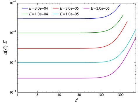
Figure 2: Hyperdiffusion profiles as a function of the spherical harmonic degree $\ell$ for the numerical simulations of Tab. 1 (Eq. 8).

While ensuring the stability of numerical models at values of Ekman and Rayleigh numbers that would normally require higher levels of truncation, the use of hyperdiffusion has some potential caveats. It potentially introduces some anisotropy between the horizontal and the radial direction as $d(\ell)$ depends on the horizontal scale only. In addition, hyperdiffusion yields an artificial viscous heating that can affect the heat transport balance (Glatzmaier, 2002). However the amplitudes employed here are relatively weak and hyperdiffusivity seems to mainly act as a low pass-filter on the small-scale convective structures close to the outer boundary. As a reliability check, the initial amplitudes of hyperdiffusion have been reduced stepwise when the simulations reached a statistically steady-state without qualitatively affecting the results.

2.3 Parameter choice

The parameters of the five numerical models discussed here have been chosen to model the dynamics of the molecular envelope of a giant planet, within the accessible numerical parameter space. Tab. 1 summarizes this parameter choice. The values of $E$ and $Ra^{*}$ explored here are far from estimated values for a gas giant planet. Computational resolution limits us to a minimum Ekman number that is roughly 10 orders of magnitude larger than that for Jupiter. The Ekman number has been gradually lowered, spanning the range from $E=3\times 10^{-4}$ to $E=3\times 10^{-6}$. The values of $Ra^{*}$ have been tuned to obtain zonal Rossby number profiles of similar amplitudes for the different Ekman numbers. To maintain zonal flow velocities comparable to Saturn ($Ro\simeq 0.05$ at the equator) the model $Ra^{*}$ values decrease with decreasing $E$. However, $Ra^{*}$ is still orders of magnitude greater than planetary values for the case with the lowest Ekman number. In contrast with our previous parameter studies, which were dedicated to the influence of $Ra^{*}$ on the zonal flow regime (Gastine et al., 2013, 2014), here we consider numerical models with similar Rossby numbers and focus on the influence of the Ekman number. The Prandtl number is set to 1 for $E\geq 10^{-4}$ and then successively lowered in the most demanding cases to ensure a quicker nonlinear saturation. We employ a larger aspect ratio of $\eta=0.85$ than in our previous studies (Gastine and Wicht, 2012; Gastine et al., 2013) which is known to promote the formation of multiple high latitude jets (e.g. Christensen, 2001; Heimpel et al., 2005; Heimpel and Aurnou, 2007).

The thickness of this convective layer exceeds estimates of the zonal flow depth of Jupiter ($\sim 0.95\,R_{J}$) but is comparable to estimated values for Saturn ($\sim 0.85\,R_{S}$, see Liu et al., 2008; Nettelmann et al., 2013). Using these estimates of the zonal flow depth as lengthscales, $\nu=3\times 10^{-7}~{}\text{m}^{2}/\text{s}$ as a typical value for the kinematic viscosity in the molecular envelope and $\Omega_{J}=1.75\times 10^{-4}~{}\text{s}^{-1}$ ($\Omega_{S}=1.64\times 10^{-4}~{}\text{s}^{-1}$) allow to estimate the Ekman numbers for Jupiter ($E=10^{-16}$) and Saturn ($E=10^{-17}$). According to the internal models by (French et al., 2012), the thermal diffusivity varies from $\kappa=3\times 10^{-7}~{}\text{m}^{2}/\text{s}$ to $\kappa=2\times 10^{-6}~{}\text{m}^{2}/\text{s}$ in Jupiter’s molecular envelope, which yields $0.15<Pr<1$. A direct estimate of $Ra^{*}$ for Jupiter and Saturn is not accessible as the value of the superadiabatic entropy contrast $\Delta s$ is not known. However, following Gastine et al. (2013), this parameter can be indirectly inferred from the modified flux-based Rayleigh number $Ra_{q}^{*}=Ra^{*}\,Nu^{*}=\alpha gq/\rho c_{p}\Omega^{3}d^{2}$ and the heat transport scaling law that relates the modified Nusselt number $Nu^{*}$ to $Ra_{q}^{*}$ via $Nu^{*}=0.076\,(Ra_{q}^{*})^{0.53}$ (e.g. Christensen, 2002; Gastine and Wicht, 2012). The values given in Tab. 2 then yield $Ra^{*}=2\times 10^{-4}$ and $Ra^{*}=6\times 10^{-5}$ for Jupiter and Saturn, respectively.

Table 2: Physical properties and values assumed for Jupiter and Saturn (Hanel et al., 1981; Guillot, 1999; French et al., 2012).

quantity	meaning (units)	Jupiter	Saturn
$d$	Lengthscale (m)	$0.05\,R_{J}=3.5\times 10^{6}$	$0.15\,R_{S}=8.7\times 10^{6}$
$\Omega$	Rotation rate (s-1)	$1.75\times 10^{-4}$	$1.64\times 10^{-4}$
$q$	Heat flux (W/m2)	5.5	2
$\rho$	Density (kg/m3)	250	330
$\alpha$	Thermal expansivity (K-1)	$9\times 10^{-5}$	$3\times 10^{-4}$
$g$	Gravity (m/s2)	25	12
$c_{p}$	Heat capacity (J/kg/K)	$1.2\times 10^{4}$	$1.2\times 10^{4}$

All the simulations have a polytropic index $m=2$ and a strong density contrast of $N_{\rho}=5$, which corresponds to $\rho_{\text{bot}}/\rho_{\text{top}}\simeq 150$. Due to the numerical limitations, this stratification is still weaker than the actual density contrast of the envelope of a giant planet: for instance, Saturn’s model by Nettelmann et al. (2013) suggests $N_{\rho}=7.4$ between $0.85\,R_{S}$ and the 1 bar level (see also Guillot, 1999). The most demanding setup explored here is similar to the case F computed by Jones and Kuzanyan (2009), albeit with a smaller Ekman number and stronger zonal flows ($Ro\sim 0.05$ compared to $Ro\sim 0.01$)

The numerical models with $E\geq 10^{-4}$ have been initiated from a random entropy perturbation superimposed on the conductive thermal state. The converged solutions of these runs have then been used as a starting condition for the more demanding cases, the Ekman number being lowered in stages. All the cases were run for at least 0.5 viscous diffusion time, ensuring that a statistical steady state has been reached.

3 Results of the numerical models

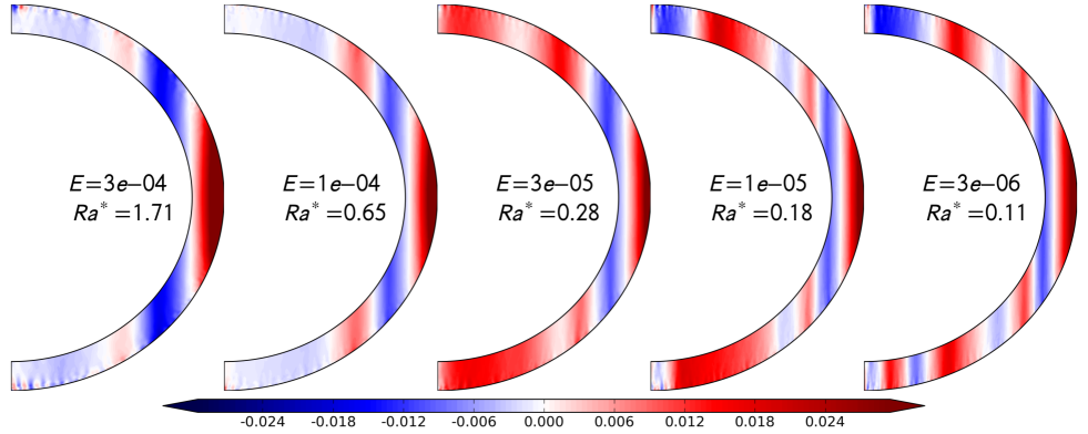
Figure 3: Snapshots of zonally averaged azimuthal velocity in the meridian plane for the numerical models of Tab. 1. Velocities are expressed in Rossby number units (i.e. $u_{\phi}/\Omega r_{o}$) and colorscales are centered around zero: prograde (retrograde) jets are rendered in red (blue). In all cases, the prograde contours have been truncated in amplitude to emphasize the structure of the secondary jets.

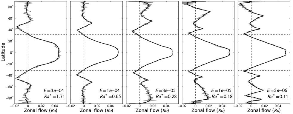
Figure 4: Surface zonal flow profiles of the numerical models of Tab. 1 (expressed in units of $Ro=u_{\phi}/\Omega r_{o}$). The grey lines correspond to the snapshots displayed in Fig. 3, while the black lines correspond to time-averaged zonal flows. On each panel, the location of the tangent cylinder is marked by the two horizontal dashed lines.

Fig. 3 shows the zonal flow structure for the five Ekman numbers employed here. The values of $Ra^{*}$ are set to keep the Rossby number at an approximately constant value. Fig. 4 portrays the corresponding latitudinal profiles of the surface zonal flows. For $E\geq 10^{-4}$ (the two first panels), the main prograde equatorial jet is flanked by retrograde zonal flows attached to the tangent cylinder. At mid-latitudes (i.e. $\theta\simeq\pm 50-60^{\circ}$) a pair of weak prograde jets develops in a similar way to our previous thicker-shell simulations (Gastine and Wicht, 2012). Typical of strongly stratified numerical models, the amplitude of the main equatorial jet is significantly larger than those of the secondary jets ($Ro\simeq 0.05$ at the equator compared to $Ro\simeq 0.01$ at $\theta\pm 45^{\circ}$). While the zonal winds are dominated by geostrophic flows, some ageostrophic features are discernable at high latitudes, especially near the outer boundary. These small-scale structures are strongly time-dependent and live on a typical convective turnover timescale. These features are responsible for the time-dependence visible in the surface zonal flow profiles (grey lines in Fig. 4) but disappear when time-averaged zonal flows are considered (black lines in Fig. 4). The geostrophic zonal flow profiles are consistent with the results of previous anelastic models by Jones and Kuzanyan (2009) and Gastine and Wicht (2012). Kaspi et al. (2009) and Showman et al. (2011) developed a modified anelastic approach that neglects viscous heating but includes a more realistic equation of state. In their models at $E\simeq 10^{-4}$, the zonal flows show a significant variation in the direction of the rotation axis, in contrast with our findings (and Jones and Kuzanyan, 2009; Gastine and Wicht, 2012). A possible explanation for this difference might come from the different heating mode employed in the different models. While, following Jones and Kuzanyan (2009), we adopt here a fixed entropy contrast, Kaspi et al. (2009) used flux-boundary conditions and internal heating. This yields significant latitudinal entropy contrasts which promotes baroclinic and ageostrophic zonal flows via the thermal-wind balance:

$$2\dfrac{\partial u_{\phi}}{\partial z}\simeq Ra^{*}\dfrac{r_{o}^{2}}{r^{3}}\dfrac{\partial s}{\partial\theta}.$$ (9)

In contrast, the latitudinal variation of entropy remains weak in our model leading to the nearly perfectly geostrophic zonal flows ($\partial u_{\phi}/\partial z\simeq 0$) shown in Fig. 3.

For the intermediate cases with $E=3\times 10^{-5}$ and $E=10^{-5}$ (third and fourth panels), additional jets start to appear at mid and high latitudes. The secondary jets already visible in the previous cases with $E\geq 10^{-4}$ are gradually squeezed towards lower latitudes. Some of the simulations shown here have a higher number of jets in one hemisphere (here the southern hemisphere). As reported by Jones and Kuzanyan (2009), this symmetry breaking is quite common in the multiple-jets regime and is sensitive to the initial conditions used in the numerical models (for another example of such an asymmetry, see the $\eta=0.9$ case by HA07). At $E=3\times 10^{-6}$ (last panels), the multiple jets inside the tangent cylinder are well-delimited and reach an amplitude of $Ro\simeq 0.015-0.02$. The number of jets is still smaller than observed on Saturn. This may be due to the model Ekman number which, even at the computationally challenging value of $E=3\times 10^{-6}$, is still orders of magnitude greater than estimates of $E$ for giant planets (Tab. 1). Nevertheless, it is evident from Fig. 4 that the jet wavelength of our models is approaching an asymptotic value with decreasing Ekman number. Thus, we find that the latitudinal extent of the zonal flows and the relative amplitude of equatorial to secondary jets shows some similarities with Saturn’s surface winds (see Fig. 1).

4 Zonal flow scaling in compressible convection

4.1 Jet scaling in quasi-geostrophic turbulence

In a typical three-dimensional turbulent flow, the energy directly cascades from large-scale eddies to smaller-scale structures. However, due to the dominance of the Coriolis force, rapidly-rotating flows are strongly anisotropic. The turbulent structures are aligned with the rotation axis and form a quasi-geostrophic flow which approximately satisfies the Taylor-Proudman theorem. This quasi-two-dimensionalisation of the flow promotes the development of an inverse energy cascade which transfers energy from small-scale to larger-scale structures (e.g. Sukoriansky et al., 2007). In addition, due to the latitude-dependent effect of the Coriolis force, the flows can also be characterized by Rossby waves with wavenumbers that depend on the so-called $\beta$-effect. In a 2-D shallow layer model (under the $\beta$-plane approximation), the $\beta$-effect can be attributed to the latitudinal variations of the Coriolis parameter $f=2\Omega\sin\theta$, leading to $\beta=1/r_{o}\,(df/d\theta)$ where $\theta$ is the latitude and $r_{o}$ is the radius of the 2D spherical surface (e.g. Williams, 1978). Alternatively, in a quasi-geostrophic flow that develops in a 3D spherical shell, the topographic $\beta$-effect depends on the relative height variation of the shell with the distance to the rotation axis: $\beta=2\Omega\,(d\ln h/ds)$, where $s$ is the cylindrical radius and $h$ is the height of the spherical shell (e.g. Aubert et al., 2003; Schaeffer and Cardin, 2005, HA07). In his original derivation, Rhines (1975) proposed that the inverse cascade ceases at a typical lengthscale defined by $L_{\beta}\sim k_{\beta}^{-1}\sim(2U_{\text{rms}}/\beta)^{1/2}$, subsequently referred to as the Rhines scale. In other words, $k_{\beta}$ separates the spectrum on turbulence (smaller scales with $k>k_{\beta}$) and Rossby waves (larger scales with $k<k_{\beta}$). Furthermore, $k_{\beta}$ is related to the zonation of the turbulent flow which forms alternating jets of typical width $k_{\beta}^{-1}$. The interpretation of the Rhines wavelength is however still debated and the precise role played by the inverse cascade on the zonation mechanism remains controversial (Sukoriansky et al., 2007; Tobias et al., 2011; Srinivasan and Young, 2012). Despite these uncertainties, this lengthscale plays a major role in many natural systems encompassing oceanic circulation (e.g. Vallis and Maltrud, 1993); atmosphere dynamics (e.g. Held and Larichev, 1996; Schneider, 2004) and circulation in the gas giants atmospheres (Vasavada and Showman, 2005, HA07).

In a compressible fluid, the exact definition of the $\beta$ parameter that enters the Rhines wavelength is, however, not clear. Indeed, Evonuk (2008) and Glatzmaier et al. (2009) pointed out that the compressibility adds a new vorticity source that could potentially alter the definition of $L_{\beta}$. In their two-dimensional numerical models, the flow is cylindrical, with no boundary curvature effect (i.e. $\beta=0$) and the density only varies in a direction perpendicular to the rotation axis. In this particular setup, $L_{\beta}$ can thus be simply replaced by $L_{\rho}=(2U_{\text{rms}}/\beta_{\rho})^{1/2}$, with $\beta_{\rho}=2\Omega\,(d\ln\tilde{\rho}/ds)$, $s$ being the cylindrical radius (see also Verhoeven and Stellmach, 2014). In a 3-D spherical shell, however, this compressional Rhines scale is unlikely to be directly applicable. First, the height of the container varies with the distance to the rotation axis and the classical topographic $\beta$ will therefore play a role. Secondly, the density varies with the spherical radius $r$ and the definition of $L_{\rho}$ based on $s$ must take this into account (Jones and Kuzanyan, 2009).

4.2 $\beta$-effect in a compressible fluid

A formulation of the $\beta$-parameter that depends on the variation of the axially integrated mass with distance from the rotation axis was proposed by Ingersoll and Pollard (1982) for quasi-geostrophic flows. Here we verify this scaling argument by deriving the compressional $\beta$-parameter and Rhines scale in a spherical shell in a consistent way with the momentum equation (3). To do this we first examine the flow structure in the compressible quasi-geostrophic limit. Taking the curl of Eq. (3) gives the following vorticity equation

$$\dfrac{D\mathchoice{\mbox{\boldmath$\displaystyle\omega$}}{\mbox{\boldmath$\textstyle\omega$}}{\mbox{\boldmath$\scriptstyle\omega$}}{\mbox{\boldmath$\scriptscriptstyle\omega$}}}{Dt}+\mathchoice{\mbox{\boldmath$\displaystyle\omega$}}{\mbox{\boldmath$\textstyle\omega$}}{\mbox{\boldmath$\scriptstyle\omega$}}{\mbox{\boldmath$\scriptscriptstyle\omega$}}(\mathchoice{\mbox{\boldmath$\displaystyle\nabla$}}{\mbox{\boldmath$\textstyle\nabla$}}{\mbox{\boldmath$\scriptstyle\nabla$}}{\mbox{\boldmath$\scriptscriptstyle\nabla$}}\cdot\mathchoice{\mbox{\boldmath$\displaystyle u$}}{\mbox{\boldmath$\textstyle u$}}{\mbox{\boldmath$\scriptstyle u$}}{\mbox{\boldmath$\scriptscriptstyle u$}})-(\mathchoice{\mbox{\boldmath$\displaystyle\omega$}}{\mbox{\boldmath$\textstyle\omega$}}{\mbox{\boldmath$\scriptstyle\omega$}}{\mbox{\boldmath$\scriptscriptstyle\omega$}}\cdot\mathchoice{\mbox{\boldmath$\displaystyle\nabla$}}{\mbox{\boldmath$\textstyle\nabla$}}{\mbox{\boldmath$\scriptstyle\nabla$}}{\mbox{\boldmath$\scriptscriptstyle\nabla$}})\mathchoice{\mbox{\boldmath$\displaystyle u$}}{\mbox{\boldmath$\textstyle u$}}{\mbox{\boldmath$\scriptstyle u$}}{\mbox{\boldmath$\scriptscriptstyle u$}} =2\left[\dfrac{\partial\mathchoice{\mbox{\boldmath$\displaystyle u$}}{\mbox{\boldmath$\textstyle u$}}{\mbox{\boldmath$\scriptstyle u$}}{\mbox{\boldmath$\scriptscriptstyle u$}}}{\partial z}-(\mathchoice{\mbox{\boldmath$\displaystyle\nabla$}}{\mbox{\boldmath$\textstyle\nabla$}}{\mbox{\boldmath$\scriptstyle\nabla$}}{\mbox{\boldmath$\scriptscriptstyle\nabla$}}\cdot\mathchoice{\mbox{\boldmath$\displaystyle u$}}{\mbox{\boldmath$\textstyle u$}}{\mbox{\boldmath$\scriptstyle u$}}{\mbox{\boldmath$\scriptscriptstyle u$}})\mathchoice{\mbox{\boldmath$\displaystyle e_{z}$}}{\mbox{\boldmath$\textstyle e_{z}$}}{\mbox{\boldmath$\scriptstyle e_{z}$}}{\mbox{\boldmath$\scriptscriptstyle e_{z}$}}\right]$$ (10)

$$+\mathchoice{\mbox{\boldmath$\displaystyle\nabla$}}{\mbox{\boldmath$\textstyle\nabla$}}{\mbox{\boldmath$\scriptstyle\nabla$}}{\mbox{\boldmath$\scriptscriptstyle\nabla$}}\times\left(Ra^{*}\dfrac{r_{o}^{2}}{r^{2}}s\,\mathchoice{\mbox{\boldmath$\displaystyle e_{r}$}}{\mbox{\boldmath$\textstyle e_{r}$}}{\mbox{\boldmath$\scriptstyle e_{r}$}}{\mbox{\boldmath$\scriptscriptstyle e_{r}$}}+\dfrac{E}{\tilde{\rho}}\mathchoice{\mbox{\boldmath$\displaystyle\nabla$}}{\mbox{\boldmath$\textstyle\nabla$}}{\mbox{\boldmath$\scriptstyle\nabla$}}{\mbox{\boldmath$\scriptscriptstyle\nabla$}}\cdot\mathsf{S}\right),$$

where $D/Dt$ corresponds to the substantial time derivative. In the limit of small Ekman and Rossby numbers, the first-order contribution of this equation comes from the Coriolis force. Retaining only the first term on the right hand side of Eq. (10), and using the continuity equation (2), in cylindrical coordinates $(s,\phi,z)$, one thus obtains in the geostrophic limit

$$\dfrac{\partial u_{s}}{\partial z}=\dfrac{\partial u_{\phi}}{\partial z}=0\quad;\quad\dfrac{\partial u_{z}}{\partial z}=-\dfrac{d\ln\tilde{\rho}}{dr}u_{r}.$$ (11)

This is the Taylor-Proudman theorem reformulated for a compressible fluid (see also Tortorella, 2005; Jones and Kuzanyan, 2009). $u_{\phi}$ and $u_{s}$ are $z$-independent as in the Boussinesq approximation, while $u_{z}$ depends on $z$, owing to the strong density gradients close to the surface. The first-order flow contributions can thus be expressed as $u_{s}(s,\phi)$, $u_{\phi}(s,\phi)$ and $u_{z}(s,\phi,z)$. This also means that the $z$-vorticity component (i.e. $\omega_{z}=(\mathchoice{\mbox{\boldmath$\displaystyle\nabla$}}{\mbox{\boldmath$\textstyle\nabla$}}{\mbox{\boldmath$\scriptstyle\nabla$}}{\mbox{\boldmath$\scriptscriptstyle\nabla$}}\times u)_{z}$) is a function of $s$ and $\phi$ only in the geostrophic limit.

To derive the compressible formulation of the $\beta$-effect, we focus on the $z$-component of Eq. (10). Following Rhines (1975), we first establish the dispersion relation for pure compressible Rossby waves, using the linearised $z$-vorticity equation without source and dissipation terms. We consider in the following the dimensional formulation of this equation to ease further comparisons with observations.

$$\dfrac{\partial\omega_{z}}{\partial t}=2\Omega\left(\dfrac{\partial u_{z}}{\partial z}+\mathchoice{\mbox{\boldmath$\displaystyle u$}}{\mbox{\boldmath$\textstyle u$}}{\mbox{\boldmath$\scriptstyle u$}}{\mbox{\boldmath$\scriptscriptstyle u$}}\cdot\mathchoice{\mbox{\boldmath$\displaystyle\nabla$}}{\mbox{\boldmath$\textstyle\nabla$}}{\mbox{\boldmath$\scriptstyle\nabla$}}{\mbox{\boldmath$\scriptscriptstyle\nabla$}}\ln\tilde{\rho}\right).$$ (12)

Expanding the density gradient in cylindrical coordinates then leads to

$$\dfrac{\partial\omega_{z}}{\partial t}=2\Omega\left(\dfrac{\partial u_{z}}{\partial z}+\dfrac{1}{\tilde{\rho}}\dfrac{\partial\tilde{\rho}}{\partial s}u_{s}+\dfrac{1}{\tilde{\rho}}\dfrac{\partial\tilde{\rho}}{\partial z}u_{z}\right).$$ (13)

We then multiply this equation by $\tilde{\rho}$ and average over the height $h$ of the spherical shell, where $h=2\sqrt{\smash{r_{o}^{2}}-s^{2}}$ outside the tangent cylinder and $h=\sqrt{\smash{r_{o}^{2}}-s^{2}}-\sqrt{\smash{r_{i}^{2}}-s^{2}}$ inside

$$\dfrac{1}{h}\int_{h}\dfrac{\partial\tilde{\rho}{\omega}_{z}}{\partial t}dz=2\Omega\left(\dfrac{1}{h}\int_{h}\dfrac{\partial\tilde{\rho}u_{z}}{\partial z}dz+\dfrac{1}{h}\int_{h}\dfrac{\partial\tilde{\rho}}{\partial s}u_{s}dz\right).$$ (14)

Using the anelastic Taylor-Proudman theorem given in Eq. (11), $u_{s}$ and $\omega_{z}$ can be taken out of the integrals, leading to

$$\dfrac{M}{h}\dfrac{\partial\omega_{z}}{\partial t}=2\Omega\left(\underbrace{\dfrac{1}{h}\int_{h}\dfrac{\partial\tilde{\rho}u_{z}}{\partial z}dz}_{(a)}+\underbrace{\dfrac{u_{s}}{h}\int_{h}\dfrac{\partial\tilde{\rho}}{\partial s}dz}_{(b)}\right),$$ (15)

where $M=\int_{h}\tilde{\rho}dz$ is the integrated mass along the axial direction. The first integral in the right hand side of this equation is a surface integral that can be simplified using the impermeable flow boundary condition $u_{r}[r_{i},r_{o}]=0$. In cylindrical coordinates, this leads to

$$\cos\theta\,u_{z}(r=[r_{i},r_{o}])+\sin\theta\,u_{s}(r=[r_{i},r_{o}])=0.$$ (16)

Using $\cos\theta=z/r$ and $\sin\theta=s/r$ then leads to

$$(a)=\left\{\begin{aligned} &-\dfrac{\rho_{o}s}{r_{o}^{2}-s^{2}}\bar{u}_{s}\,\text{for}\,s\geq r_{i},\\ &\dfrac{s\left(\rho_{i}\sqrt{\frac{r_{o}^{2}-s^{2}}{r_{i}^{2}-s^{2}}}-\rho_{o}\sqrt{\frac{r_{i}^{2}-s^{2}}{r_{o}^{2}-s^{2}}}\,\right)}{\sqrt{r_{o}^{2}-s^{2}}-\sqrt{r_{i}^{2}-s^{2}}}\bar{u}_{s}\,\text{for}\,s<r_{i},\end{aligned}\right.$$ (17)

where $\rho_{o}$ and $\rho_{i}$ are the density at outer and inner radii, respectively. The second integral of Eq. (15) can be rearranged using the Leibniz rule of differentiation under the integral sign:

$$\dfrac{\partial M}{\partial s}=\dfrac{\partial}{\partial s}\int_{h}\tilde{\rho}dz=\left[\tilde{\rho}\dfrac{dh}{ds}\right]_{h}+\int_{h}\dfrac{\partial\tilde{\rho}}{\partial s}dz.$$ (18)

One thus gets

$$(b)=\left\{\begin{aligned} &\dfrac{1}{h}\dfrac{\partial M}{\partial s}\bar{u}_{s}+\dfrac{\rho_{o}s}{r_{o}^{2}-s^{2}}\bar{u}_{s}\,\text{for}\,s\geq r_{i},\\ &\dfrac{1}{h}\dfrac{\partial M}{\partial s}\bar{u}_{s}-\dfrac{s\left(\rho_{i}\sqrt{\frac{r_{o}^{2}-s^{2}}{r_{i}^{2}-s^{2}}}-\rho_{o}\sqrt{\frac{r_{i}^{2}-s^{2}}{r_{o}^{2}-s^{2}}}\,\right)}{\sqrt{r_{o}^{2}-s^{2}}-\sqrt{r_{i}^{2}-s^{2}}}\bar{u}_{s}\,\text{for}\,s<r_{i}.\end{aligned}\right.$$ (19)

The sum of $(a)$ and $(b)$ simply yields

$$\dfrac{\partial\omega_{z}}{\partial t}=\beta_{\rho}u_{s}\quad\text{with}\quad\beta_{\rho}=\dfrac{2\Omega}{M}\dfrac{\partial M}{\partial s}.$$ (20)

In a compressible fluid, the $\beta$-effect therefore depends on the variation of the $z$-integrated mass with the distance to the rotation axis. This confirms the expression suggested by Ingersoll and Pollard (1982) for a quasi-geostrophic anelastic fluid. In the Boussinesq limit, $\beta_{\rho}$ reduces to the topographic $\beta$ effect derived by HA07:

$$\left\{\begin{aligned} \dfrac{\beta_{h}}{2\Omega}=\dfrac{1}{h}\dfrac{dh}{ds}&=-\dfrac{s}{r_{o}^{2}-s^{2}};\quad s\geq r_{i},\\ \dfrac{\beta_{h}}{2\Omega}=\dfrac{1}{h}\dfrac{dh}{ds}&=\dfrac{s}{\sqrt{\smash{r_{o}^{2}}-s^{2}}\sqrt{\smash{r_{i}^{2}}-s^{2}}};\quad s<r_{i}.\\ \end{aligned}\right.$$ (21)

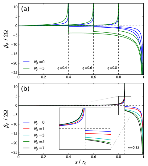
Figure 5: Upper panel: $\beta_{\rho}$ profiles for different spherical shell geometries $\eta=[0.4,0.6,0.8]$ with $N_{\rho}=0$ and $N_{\rho}=5$. Lower panel: $\beta_{\rho}$ profiles for different density stratifications $N_{\rho}=[0,1,3,5,7]$ with $\eta=0.85$. On each panel, the location of the tangent cylinder is marked by a vertical dashed line.

Figure 5 shows some examples of such $\beta_{\rho}$ profiles for different spherical shell geometries and density stratifications. Outside the tangent cylinder, the integrated mass decreases when going away from the rotation axis resulting in negative $\beta_{\rho}$. The opposite happens inside the tangent cylinder. The differences with the classical topographic $\beta_{h}$ profiles (blue curves in Fig. 5a) are more pronounced in the case of a relatively thick spherical shell ($\eta=0.4$ or $\eta=0.6$). For a thinner shell ($\eta=0.8$), this difference fades away for $s<r_{i}$ but $\beta_{\rho}$ is still significantly larger in amplitude than $\beta_{h}$ outside the tangent cylinder due to the strong density gradient in the equatorial region. This is highlighted in the lower panel of Fig. 5 where we consider several density contrasts in a thin spherical shell with $\eta=0.85$. In such a thin shell, $\beta_{\rho}$ increases regularly with $N_{\rho}$ outside the tangent cylinder. Inside, the profiles are nearly unaffected by the density stratification except in the immediate vicinity of the tangent cylinder.

4.3 Compressible Rhines scale

The Rhines scale is obtained when the phase velocity of Rossby waves equals the mean rms flow velocity. We thus need to determine the dispersion relation of the anelastic Rossby wave. With the compressible Taylor-Proudman theorem given in Eq. (11), the continuity equation $\mathchoice{\mbox{\boldmath$\displaystyle\nabla$}}{\mbox{\boldmath$\textstyle\nabla$}}{\mbox{\boldmath$\scriptstyle\nabla$}}{\mbox{\boldmath$\scriptscriptstyle\nabla$}}\cdot\tilde{\rho}\mathchoice{\mbox{\boldmath$\displaystyle u$}}{\mbox{\boldmath$\textstyle u$}}{\mbox{\boldmath$\scriptstyle u$}}{\mbox{\boldmath$\scriptscriptstyle u$}}=0$ applied to the first-order flow can be rewritten as

$$\dfrac{1}{s}\dfrac{\partial su_{s}}{\partial s}+\dfrac{1}{s}\dfrac{\partial u_{\phi}}{\partial\phi}=0.$$ (22)

Introducing a streamfunction $\psi$, $u_{s}$ and $u_{\phi}$ are expressed as

$$u_{s}=\dfrac{1}{s}\dfrac{\partial\psi}{\partial\phi}\quad\text{and}\quad u_{\phi}=-\dfrac{\partial\psi}{\partial s}.$$ (23)

Noting that $\omega_{z}=-\Delta\psi$, the linear inviscid $z$-vorticity equation (Eq. 20) can be rewritten as

$$\dfrac{\partial\Delta\psi}{\partial t}=-\dfrac{\beta_{\rho}}{s}\dfrac{\partial\psi}{\partial\phi}.$$ (24)

Looking for plane waves with $\psi=\hat{\psi}\exp i(\mathchoice{\mbox{\boldmath$\displaystyle k$}}{\mbox{\boldmath$\textstyle k$}}{\mbox{\boldmath$\scriptstyle k$}}{\mbox{\boldmath$\scriptscriptstyle k$}}\cdot\mathchoice{\mbox{\boldmath$\displaystyle r$}}{\mbox{\boldmath$\textstyle r$}}{\mbox{\boldmath$\scriptstyle r$}}{\mbox{\boldmath$\scriptscriptstyle r$}}-\omega t)$, we obtain the following dispersion relation

$$\omega=-\dfrac{\beta_{\rho}k_{\phi}}{k^{2}},$$ (25)

where $k^{2}=k_{s}^{2}+k_{\phi}^{2}$. This is identical to the dispersion relation of Rhines (1975), except that $\beta_{\rho}$ replaces Rhines’ $\beta$-plane parameter for 2-D turbulence. Due to the sign change of $\beta_{\rho}$ at the tangent cylinder (see Fig. 5), the anelastic Rossby waves propagate westward inside the tangent cylinder and eastward outside in a similar way as the classical Rossby waves.

Retaining buoyancy driving and viscosity in the vorticity equation (12) would lead to a set of coupled differential equations. There is no easy way to derive the exact dispersion relation of the thermal Rossby waves in spherical geometry with $\tilde{\rho}$, $\tilde{T}$ and $s$ varying with radius. A possible workaround to establish an approximate dispersion relation would be to consider an anelastic annulus in which the convective forcing is maintained in the $s$ direction. In addition, the diffusion operators are more complicated than a simple Laplacian in an anelastic fluid as they involve partial derivatives of $\tilde{\rho}$. As a first-order approximation and in analogy with the Busse annulus, we can nevertheless speculate that an additional factor that involves the Prandtl number might enter the dispersion relation of the thermal Rossby waves (e.g. Busse, 1970). An approximate dispersion relation for compressible thermal Rossby waves would then be

$$\omega_{th}\sim-\dfrac{\beta_{\rho}k_{\phi}}{(1+Pr)\,k^{2}}.$$ (26)

Comparing with Eq. (25) we see that a correction factor to the classical Rossby waves is therefore moderate for $Pr=0.1-1$, which is relevant for the gas giants. Owing to the uncertainties associated with the derivation of Eq. (26) and the rather small correction factor, we will therefore work in the following with the dispersion relation of classical Rossby waves (Eq. 25).

Following Rhines (1975), the phase velocity (given by $v_{p}=\Re(\omega/k)$) is obtained by taking an average orientation of the wave crests. This leads to $v_{p}\sim\beta_{\rho}/2k^{2}$. Equating $v_{p}$ with $U_{\text{rms}}$ yields the compressible Rhines wavenumber $k_{\beta}$ given by

$$k_{\beta}=\sqrt{\dfrac{|\beta_{\rho}|}{2U_{\text{rms}}}}=\sqrt{\dfrac{\Omega}{U_{\text{rms}}}\left|\dfrac{\partial\ln M}{\partial s}\right|}.$$ (27)

From that, the Rhines wavelength in the $s$ direction is given by

$$\lambda_{g}=\dfrac{2\pi}{k_{\beta}}.$$ (28)

Note that HA07 used the Rhines wavelength in the $\theta$ direction to ease the comparison with the planetary observations. Here we employ the cylindrical coordinates which are more natural in the quasi-geostrophic limit.

5 Applications of the compressional Rhines scaling

5.1 An application to a numerical model

Figure 6: Sketch explaining the definition of the jets boundaries used in this study. The solid black line corresponds to an arbitrary surface zonal flow profile plotted against the cylindrical radius $s$, while the dotted vertical lines show the zonal flow boundaries. $\lambda_{g}$ refers to the Rhines wavelength defined in Eq. (28).

To check the influence of the compressional $\beta$-effect, we test the applicability of the Rhines scaling to our numerical results. As visible on Figs. 3 and 4, the different numerical models have comparable Rossby numbers. As these models also share the same reference density profile, the Rhines scaling would therefore predict the same number of jets in these different models according to Eq. (27). In contrast, we observe a gradual increase of the number of jets when the Ekman number is decreased (Fig. 3). Although this might challenge the applicability of the Rhines scaling to our numerical models, there are some encouraging hints that suggest that the jet wavelength in our model at $E=3\times 10^{-6}$ is approaching an asymptotic state. Indeed, the zonal bands at low and mid latitudes (i.e. $|\theta|<45^{\circ}$) have already a very similar structure between the $E=10^{-5}$ and the $E=3\times 10^{-6}$ cases and only the high-latitude jets continue to further develop when decreasing the Ekman number. This indicates that our models are converging towards the saturated state of the jet wavelength suggested by the Rhines scaling for a given value of $U_{\text{rms}}/\Omega$. As a consequence we focus here on the model with the smallest Ekman number ($E=3\times 10^{-6}$).

The jet width is defined in cylindrical coordinates as the distance between two successive minima of $|\bar{u}_{\phi}|$. Here, the overbar corresponds to an azimuthal average. A jet boundary can therefore occur either at a sign change of $\bar{u}_{\phi}$ or, more rarely, at a local minimum. As shown in Fig. 6, this measured jet width corresponds to half the Rhines wavelength $\lambda_{g}/2$. Considering symmetry about the equator we take the outer boundary ($s=r_{o}$) as the center of the equatorial jet, as shown in Fig. 6.

To evaluate the jet width predicted by the Rhines scaling, the right hand side of Eq. (28) is averaged for each jet separately. Strictly speaking the total rms velocity should be considered when evaluating $k_{\beta}$. However, for comparison with the gas giants, where the zonal velocity component dominates, consideration of $\bar{u}_{\phi}$ is sufficient. In addition, we note that for our simulation at $E=3\times 10^{-6}$, the energy budget is dominated by the zonal flow contribution ($E_{\text{zon}}/E_{\text{tot}}\simeq 0.97$), so that using $\bar{u}_{\phi}$ does not significantly affect the results.

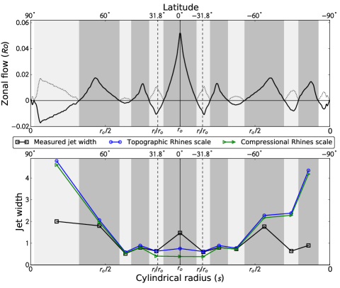
Figure 7: Upper panel: surface zonal flow profiles plotted against the cylindrical radius $s$ for a numerical model with $E=3\times 10^{-6}$, $N_{\rho}=5$, $\eta=0.85$, $m=2$ (last panels of Figs. 3-4). Lower panel: comparison of measured and predicted jet width for this numerical model. The jets boundaries (defined as on Fig. 6) are successively highlighted by light and dark grey shaded area. The location of the tangent cylinder is marked by vertical dashed lines: $r_{i}/r_{o}=0.85$ corresponds to a latitude of $31.8^{\circ}$.

The upper panel of Fig. 7 shows the surface zonal flow profile of this numerical model as a function of $s$. This simulation has several jets inside the tangent cylinder which are highlighted by different grey shading. The lower panel of Fig. 7 shows the comparison between these measured zonal flow widths and the theoretical values based on the Rhines scale. Inside the tangent cylinder, due to the similarities between $\beta_{\rho}$ and $\beta_{h}$ (see Fig. 5b), topographic and compressional Rhines scale give very similar predictions. Both profiles are in relatively good agreement with the observed widths of the mid-latitude jets (i.e. $r_{o}/2<s<r_{i}/r_{o}$ or $30^{\circ}<|\theta|<60^{\circ}$). As $\beta_{\rho}$ tends to zero at the poles, the Rhines wavelength becomes very large close to the rotation axis and fails to predict the observed width of the high-latitude jets ($s<r_{o}/2$ or $\theta>60^{\circ}$). Outside the tangent cylinder, the compressional Rhines wavelength predicts a narrower jet as the topographic one, owing to $|\beta_{\rho}|>|\beta_{h}|$ there. Both underestimate the width of the equatorial jet by at least a factor of 2. This confirms previous observations by HA07 which have shown that the Rhines scale does not apply at the equator (see also Williams, 1978). The width of the equatorial jet seems instead to be largely controlled by the shell gap (e.g. Christensen, 2001; Heimpel et al., 2005; Gastine and Wicht, 2012).

5.2 An application to giant planets

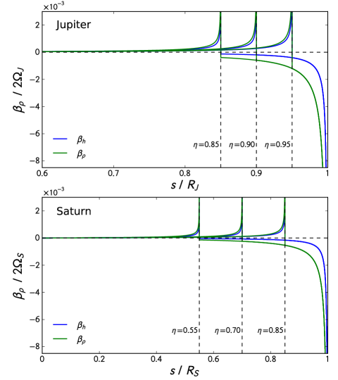
Figure 8: $\beta_{\rho}$ and $\beta_{h}$ profiles for Jupiter and Saturn (calculated from French et al., 2012; Nettelmann et al., 2013). The vertical dashed lines correspond to different possible locations of the tangent cylinder.

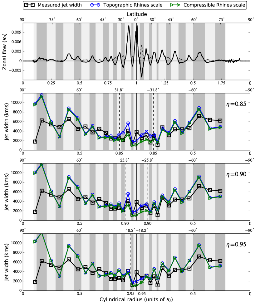
Figure 9: Upper panel: Jupiter’s zonal flow profiles from Porco et al. (2003). Lower panels: comparison of measured and predicted jet widths for three different aspect ratios: $\eta=0.85$, $\eta=0.9$ and $\eta=0.95$. The jet boundaries (defined as on Fig. 6) are successively highlighted by light and dark grey shaded area. The dashed line in the upper panel corresponds to the absolute value of the surface zonal flows. The locations of the tangent cylinders are marked by vertical dashed lines.

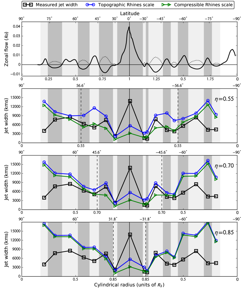
Figure 10: Upper panel: Saturn’s zonal flow profiles from Read et al. (2009). Lower panels: comparison of measured and predicted jet widths for three different aspect ratios $\eta=0.55$, $\eta=0.7$ and $\eta=0.85$. The jet boundaries (defined as on Fig. 6) are successively highlighted by light and dark grey shaded area. The dashed line in the upper panel corresponds to the absolute value of the surface zonal flows. The locations of the tangent cylinders are marked by vertical dashed lines.

The deep structure of the zonal jets in the gas giant interiors is still a matter of ongoing debates. The recent models by Kaspi et al. (2009), for instance, suggest an important variation of the zonal flow amplitude along the axis of rotation which is not captured by our numerical simulations. It is therefore not clear if the compressional Rhines scale derived within the quasi-geostrophic limit is still applicable if the zonal flows show such a pronounced $z$-dependence. Keeping this limitation in mind, we nevertheless test the applicability of the compressional Rhines scaling to giant planets.

To estimate the width of the zonal jets, we use the observed surface zonal flow profiles by Porco et al. (2003) for Jupiter and by Read et al. (2009) for Saturn (see Fig. 1). Figure 8 shows the radial distribution of $\beta_{\rho}$ determined from the 1-D interior models by French et al. (2012) and Nettelmann et al. (2013). These profiles are consistent with the strongly stratified cases (i.e. $N\rho\geq 5$) displayed in Fig. 5.

Following the same procedure as for the numerical model, we compare on Figs. 9-10 the measured jet width with the predicted values derived from the Rhines scaling (Eq. 28). Owing to the uncertainties on the depth of the zonal jets in giant planets, we consider several possible locations of the tangent cylinder. These values have been chosen to cover the actual estimated zonal flow depth, ranging from the entire molecular layer (i.e. $0.55\,R_{S}$ and $0.85\,R_{J}$) to the shallower layers predicted by Liu et al. (2008) (i.e. $0.85R_{S}$ and $0.95\,R_{J}$).

For Jupiter (Fig. 9), the influence of the compressibility on $k_{\beta}$ is difficult to disentangle from the topographic Rhines scaling except in the small region close to the tangent cylinder. In a similar way as for the numerical model, both $\beta_{\rho}$ and $\beta_{h}$ predict a much narrower equatorial jet than observed. The widths of the low-latitude off-equatorial jets (i.e. $10^{\circ}<|\theta|<30^{\circ}$) are in general better predicted by the compressional Rhines scale than by the incompressible one. The scaling of these low-latitude jets is independent of the thickness of the layer. At mid-latitudes ($30^{\circ}<|\theta|<60^{\circ}$), both profiles are generally in a good agreement with the observations. We nevertheless observe an increasing misfit at these latitudes when shallower layers are considered (visible here for the $\eta=0.95$ case). At higher latitudes ($|\theta|>60^{\circ}$), the misfit becomes larger and this can be attributed to the singularity of the Rhines scale when $|\theta|$ tends toward $90^{\circ}$. The previous study by HA07 based on the topographic $\beta$-effect showed that for Jupiter the best-fit is achieved when the tangent cylinder is located at $0.86\,R_{J}$. We find a similar result, with predicted values in good agreement with the observations when $\eta\simeq 0.85-0.9\,R_{J}$. However, the improvement of the fit in that range, compared to the shallower cases, is relatively small. It is therefore difficult to derive a strong constraint on the zonal flow depth based on Rhines scaling.

For Saturn (Fig. 10) the differences between calculated and observed values are, on average, larger. The prediction based on $\beta_{\rho}$ is in better agreement with the observations than $\beta_{h}$, except for the equatorial jet which is much narrower in the compressible case. Excluding this equatorial jet, the best-fit is obtained for the thicker layer with $\eta=0.55$. Considering a thinner shell indeed leads to much broader mid and high latitude (i.e. $|\theta|>45^{\circ}$) jets than observed.

On the other hand, if one focuses on the scaling of the equatorial jet only, the constraint on the depth of the molecular layer is quite different. In fact, in the numerical models at low Ekman numbers (i.e. $E<1\times 10^{-5}$), the latitudinal extent of the equatorial jet is always controlled by the geometry of the spherical shell in such a way that the first retrograde jet is attached to the tangent cylinder (see Fig. 4 and Christensen, 2001; Heimpel et al., 2005; Jones and Kuzanyan, 2009; Gastine and Wicht, 2012). For example, when $r_{i}/r_{o}=0.85$, the first minimum is located at $\arccos r_{i}/r_{o}\simeq 31.8^{\circ}$. Applying this geometrical argument to giant planets would lead to a transition radius around $0.96\,R_{J}$ and $0.86\,R_{S}$, in relatively close agreement with the values derived by Liu et al. (2008). This again underlines the difficulties to put a strong constraint on the depth of the zonal winds based on the Rhines scaling.

5.3 Asymptotic scaling laws

Using the compressional Rhines scaling also allows to construct an asymptotic scaling law for the number of zonal jets. This number is estimated as the ratio of the outer radius $r_{o}$ to the mean Rhines length $\langle\lambda_{g}\rangle$:

$$n_{\text{jets}}=2\dfrac{r_{o}}{\langle\lambda_{g}\rangle}=\dfrac{r_{o}}{\pi}\sqrt{\dfrac{\Omega\,d}{U_{\text{rms}}}}\sqrt{\dfrac{1}{d}\left\langle\left|\dfrac{\partial\ln M}{\partial s}\right|\right\rangle}.$$ (29)

The factor $2$ comes from the summation of the two hemispheres, and the triangular brackets denote an average value of the relative mass variation $|\partial\ln M/\partial s|$. The jet scaling thus directly involves the inverse square root of the Rossby number $Ro=U_{rms}/\Omega d$.

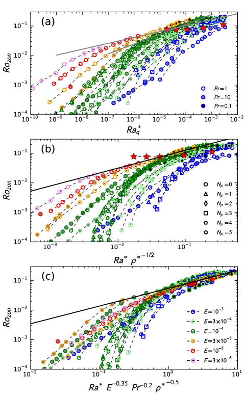
Figure 11: Different possible scaling laws for the zonal Rossby number $Ro_{\text{zon}}$ using the Boussinesq and the anelastic numerical models by Gastine and Wicht (2012); Gastine et al. (2013) and Gastine et al. (2014). a) $Ro_{\text{zon}}$ versus the modified flux-based Rayleigh number. The two solid grey lines correspond to the scaling derived by Christensen (2002) and by Gastine et al. (2013). b) $Ro_{\text{zon}}$ versus the modified Rayleigh number $Ra^{*}$. c) $Ro_{\text{zon}}$ versus $Ra^{*}\,E^{-0.35}\,Pr^{-0.2}\,{\rho^{*}}^{-0.5}$. The solid black lines in the panels b) and c) correspond to the asymptotic scaling laws. In each panel, the five red stars correspond to the numerical simulations of Tab. 1. For the three panels, the color of the rim of the symbols corresponds to the Ekman number, the inner color to the Prandtl number and the shape to the density contrast.

Several attempts have recently been made to derive an asymptotic scaling for the zonal Rossby number using 3-D numerical models of rapidly-rotating convection in spherical shells. Using Boussinesq models, Christensen (2002) suggested that the zonal Rossby number depends on the available buoyancy-power (given by the flux-based Rayleigh number $Ra_{q}^{*}$) and obeys the following scaling law:

$$Ro_{\text{zon}}=\dfrac{U_{\text{zon}}}{\Omega d}=\alpha\,\left(Ra_{q}^{*}\right)^{\beta},$$ (30)

where $(\alpha=0.65,\,\beta=1/5)$. More recently, Showman et al. (2011) and Gastine and Wicht (2012) derived similar convective power scaling laws using anelastic models of rotating convection. However, the exponents vary from $(\alpha=1,\,\beta=1/4)$ in Showman et al. (2011) to $(\alpha=2.45,\,\beta=1/3)$ in Gastine et al. (2013). The first panel of Fig. 11 shows an example of such a power-based scaling applied to the large database of Boussinesq and anelastic models of convection in rapidly-rotating spherical shells built in our previous parameter studies (Gastine and Wicht, 2012; Gastine et al., 2013, 2014). Using a spherical shell with an aspect ratio $\eta=0.6$, this database spans the range of $3\times 10^{-6}<E<10^{-3}$, $Pr\in[0.1,1,10]$ and $0<N_{\rho}<5$. As described by Showman et al. (2011), the $Ro_{\text{zon}}$ scaling undergoes several slope changes that may be attributed to some successive regime transitions. For moderate driving of convection, $Ro_{\text{zon}}$ increases relatively fast with $Ra_{q}^{*}$. The slope then gradually tapers off and seems, at first glance, to saturate at a level compatible with the $1/5$ scaling suggested by Christensen (2002) (upper gray line). However, a closer look indicates that the Ekman number dependence is not well-captured as the different lines associated with the different Ekman numbers are nearly parallel, each of them following a scaling close to $1/3$ (lower gray line). In addition, the impression of an asymptotic scaling is also artificially reinforced by the $x$-axis spanning 8 decades of $Ra_{q}^{*}$ (Yadav et al., 2013a).

Alternatively, Christensen (2002) also suggested that $Ro_{\text{zon}}$ might directly scale as a function of the modified Rayleigh number $Ra^{*}$, a proxy of the ratio between buoyancy and Coriolis force in the global force balance:

$$Ro_{\text{zon}}=\alpha\,(Ra^{*})^{\beta}.$$ (31)

Fig. 11b shows such a scaling applied to the database of Boussinesq and anelastic models. The prefactor $\alpha$ shows some dependence on the background density contrast, which can be easily captured when introducting the normalised density $\rho^{*}$ as suggested by Yadav et al. (2013b):

$$\rho^{*}=\dfrac{1}{V}\int_{v}\tilde{\rho}\,dV.$$ (32)

Using $(\rho^{*})^{-1/2}$ then allows to nicely collapse the different density stratifications for one given Ekman number (open green symbols for instance). Although the scatter is significantly reduced compared to the previous $Ra_{q}^{*}$ scaling, defining an asymptotic state remains relatively awkward. Buoyancy indeed starts to play a significant role in the force balance when $Ra^{*}$ approaches unity. This change in the force balance is accompanied by a sharp transition in the zonal flow regime when $Ra^{*}\gtrsim 1$. (Aurnou et al., 2007; Gastine et al., 2013, 2014). This is already visible on the right part of Fig. 11b where we observe a gradual flattening of the $Ro_{\text{zon}}$ scaling. We can nevertheless bound the rapidly-rotating regime to the numerical models that fulfill $Ra^{*}\,(\rho^{*})^{-1/2}<0.1$. This yields the tentative asymptotic scaling $Ro_{\text{zon}}=0.5\,(Ra^{*}/{\rho^{*}}^{1/2})^{0.6}$ shown by the solid black line in Fig. 11b. The thin shell simulations of the present study, visible as the five red stars, are however relatively far from the asymptotic scaling, suggesting a possible additional dependence on the geometry of the spherical shell.

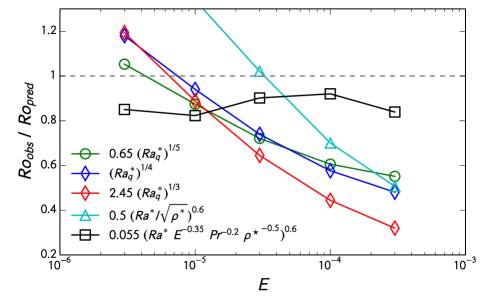
Figure 12: Test of the predictive power of different scaling laws: ratio of the actual zonal Rossby number ($Ro_{obs}$) of the different numerical models of Tab. 1 to the values predicted ($Ro_{pred}$) by different scaling laws. The horizontal dashed line corresponds to the ideal case of a perfect prediction ($Ro_{pred}=Ro_{obs}$).

This scatter around the asymptotic laws therefore suggests that the zonal flow might obey a more complex scaling. The general form of a polynomial scaling for the zonal flow component can be written as the following function of the different control parameters:

$$Ro_{\text{zon}}=\alpha\,{Ra^{*}}^{\beta}\,E^{\delta}\,Pr^{\gamma}\,{\rho^{*}}^{\epsilon}.$$ (33)

A best-fit on the database of simulations then yields:

$$Ro_{\text{zon}} =0.055\left(Ra^{*}\,E^{-0.35}\,Pr^{-0.2}\,{\rho^{*}}^{-0.5}\right)^{0.6},$$ (34)

$$=0.055\left(Ra\,E^{1.65}\,Pr^{-1.2}\,{\rho^{*}}^{-0.5}\right)^{0.6}.$$

This scaling has the same dependence on $Ra$ and $\rho^{*}$ as the previously obtained $Ra^{*}$ scaling but is not diffusivity-free anymore owing to the additional dependence on $E$ and $Pr$. Fig. 11c shows that using this scaling significantly reduces the scatter. In addition, the anelastic numerical simulations of Tab. 1 (the five red stars) now fall very close to the asymptotic scaling law. This is encouraging as it means that Eq. (34) correctly captures the dependence on the spherical shell mass and geometry.

Table 3: Table of results. The first column corresponds to the observed values for the mean surface zonal flow amplitude and the number of jets for the numerical simulation with $E=3\times 10^{-6}$, Jupiter and Saturn. The second, third and fourth columns correspond to the predicted values using the convective-power scaling by Christensen (2002), Showman et al. (2011) and Gastine and Wicht (2012). The fifth column corresponds to the $Ra^{*}$ scaling, while the last column corresponds to the predicted values using the scaling given in Eq. (34). Note that the zonal flow velocities for the numerical models have been obtained using the Saturnian rotation rate $\Omega$ and lengthscale $d$ (Tab. 2).

	Obs.	$0.65\,(Ra_{q}^{*})^{1/5}$	$(Ra_{q}^{*})^{1/4}$	$2.45\,(Ra_{q}^{*})^{1/3}$	$0.5\,(Ra^{*}/\sqrt{\rho^{*}})^{0.6}$	Eq. (34)
Zonal flow (m/s)
Simulation ($E=3\times 10^{-6}$)	110	100	90	90	60	130
Jupiter	45	3	2	1	0.3	60
Saturn	170	5	2	1	0.3	100
$n_{\text{jets}}$
Simulation ($E=3\times 10^{-6}$)	12	10	11	11	13	9
Jupiter	30	70	100	170	260	17
Saturn	17	50	80	150	220	12

Fig. 12 shows a comparison of the predicting power of these different scaling laws. The ratio of the actual $Ro_{\text{zon}}$ of the numerical models to the predicted values are plotted for the five cases of Tab. 1 for the different aforementioned asymptotic scalings. The power-based scalings fail to predict the correct Rossby number with a better accuracy than 50% for $E\geq 10^{-4}$ and gradually approach the correct values at the lowest Ekman number. The $Ra^{*}$ scaling shows a similar trend at large Ekman number and even further deviates from the correct values at low Ekman numbers. In contrast, the scaling (34) predicts the Rossby number of the five numerical models within a 20% error range without any notable remaining Ekman number dependence.

Using the values given in Tabs. 1-2 allows to extrapolate these different scalings to Jupiter and Saturn, and to evaluate the mean zonal flow amplitude and the number of jets. Confirming Showman et al. (2011) and Gastine and Wicht (2012), the power-based scalings predict zonal flow velocities around 1-5 m/s for both Jupiter and Saturn and even smaller velocities are obtained when using the $Ra^{*}$ scaling. In contrast, our new scaling (34) predicts velocities in good agreement with the observed surface mean values. The number of jets are then derived using Eq. (29) and a mean $|\partial\ln M/\partial s|$ of $2\times 10^{-7}$ m^-1 for Jupiter and $2.5\times 10^{-7}$ m^-1 for Saturn. The convective power scalings and the $Ra^{*}$ scaling overestimate the number of zonal bands by a factor of 3 to 5 for both planets. Although $n_{\text{jets}}$ is underestimated by roughly $1/2$ for both Saturn and Jupiter, the scaling (34) once again gives an improved prediction of the observed quantities.

The scaling (34) obtained from a large database of Boussinesq and anelastic models is therefore encouraging as the predicted quantities are much closer to the observed values. It is nevertheless still a tentative scaling that would require additional theoretical work to further establish the obtained exponents on physical grounds.

6 Conclusion

We have investigated several numerical simulations of rapidly-rotating convection in spherical shells. We have considered strongly stratified models with $\rho_{\text{bot}}/\rho_{\text{top}}\simeq 150$ in spherical shells with a large aspect ratio of $r_{i}/r_{o}=0.85$. Extending the previous Boussinesq study by HA07, we have explored a range of Ekman numbers ($E=3\times 10^{-4}-3\times 10^{-6}$) to allow the formation of multiple high latitude jets.

At the lowest Ekman number considered here, a strong prograde equatorial zonal flow is flanked by several alternating jets in each hemisphere. This confirms previous findings by Jones and Kuzanyan (2009) that compressible models can also maintain multiple zonal bands, provided low Ekman numbers and thin spherical shells are considered. The number of jets in our simulations is far fewer than observed for Jupiter. Smaller Ekman numbers, and even thinner shells would result in a greater number of narrower jets. However, both of these properties require computational expense that is presently impractical. Following our previous parameter studies of compressible convection (Gastine and Wicht, 2012; Gastine et al., 2013), the zonal flow profiles obtained here show many similarities with their Boussinesq counterparts (e.g. Heimpel et al., 2005, HA07). In agreement with the theory of geostrophic turbulence, the jet widths of these previous Boussinesq models have been found to scale with the Rhines length, i.e. $k_{\beta}^{-1}=\sqrt{2U/\beta}$, $\beta$ being the relative variation of the height of the spherical shell with the distance to the rotation axis (Rhines, 1975). The similarities in the zonal flow profiles of Boussinesq and anelastic models would therefore suggest that this topographic Rhines scale could be also applicable to compressible convection. This seems however at odds with the two-dimensional anelastic models by Evonuk (2008) and Glatzmaier et al. (2009) which suggested a possible modification of the Rhines lengthscale due to compressibility effects.

To address this issue, we have derived here the expression of the $\beta$-effect in a 3-D spherical shell filled with a compressible fluid. Confirming the calculations by Ingersoll and Pollard (1982), the compressional $\beta$-effect (i.e. $\beta_{\rho}$) is found to be proportional to the relative variation of the integrated mass with the distance to the rotation axis. Similarly to the classical topographic Rhines scaling (i.e. $\beta_{h}$), the compressional $\beta$-effect marks a sign reversal at the tangent cylinder. In the thin spherical shells considered here, the $\beta_{\rho}$ and $\beta_{h}$ profiles are found to be very similar inside the tangent cylinder. This explains the similarities of the high-latitude jets observed in Boussinesq and anelastic models. The main differences between topographic and compressional $\beta$-effects occur outside the tangent cylinder where the density gradient is mainly perpendicular to the rotation axis. However the Rhines scaling does not seem to be applicable there as there is only one single equatorial jet which seems to be always controlled by the geometry of the spherical shell (see also HA07). An efficient test of the compressional Rhines scale for $s>r_{i}$ would therefore require multiple zonal bands outside the tangent cylinder. While those low-latitude jets are frequently observed in the transient phases of the 3-D numerical models, they always merge on longer time resulting in one single prograde equatorial flow flanked by a retrograde jet attached to the tangent cylinder (e.g. Sun and Schubert, 1995; Christensen, 2001). Although numerically challenging, 3-D models in thicker spherical shells (i.e. $r_{i}/r_{o}\leq 0.6$) at low Ekman numbers (i.e. $E\sim 10^{-6}$) may help to check the stability of the zonal winds outside the tangent cylinder. As the differences between $\beta_{h}$ and $\beta_{\rho}$ are also more pronounced in thicker shells, it would be interesting to check the applicability of the Rhines scaling to these low-latitude jets.

The compressional $\beta$-effect has also been applied to Jupiter’s and Saturn’s surface winds. For Jupiter, $\beta_{h}$ and $\beta_{\rho}$ are relatively similar and both predict jet-widths in relatively good agreement with the observed values. For Saturn, the misfit between predictions and observations is on average larger. The compressional Rhines scale gives nevertheless a better estimate of the jet-width than the topographic one. Excluding the equatorial jet, the best fit is achieved for a range of radius ratios of $\eta\simeq 0.85-0.9$ for Jupiter and $\eta\simeq 0.55$ for Saturn. These values are on the low-side compared to the estimates derived by Liu et al. (2008). However these depths are relatively poorly constrained by the Rhines scaling owing to the small changes when the radius ratio is varied. In addition, the factor 2 entering the Rhines scale definition is not firmly established as it comes from an ad-hoc averaging of the orientation of the Rossby waves (Rhines, 1975). Sukoriansky et al. (2007) therefore argues that this factor should be replaced by a rather elusive coefficient of proportionality. It is therefore difficult to put a strong constraint on the zonal flow depth based on $\beta_{\rho}$ only. Using the compressional Rhines scale also allows to construct an asymptotic scaling for the number of zonal jets. However, estimating this number requires to employ an asymptotic scaling for the zonal flow amplitude. The disagreement between the different buoyancy power scalings published to date suggests that the zonal flow might obey a more complex scaling. Thus, we propose a simple best-fit scaling law that successfully predicts the correct zonal flow amplitude and number of bands for both the numerical models and the gas giant planets. Although encouraging, the predicted dependence on the control parameters $Ra^{*}$, $E$ and $Pr$ is still tentative and needs further theoretical investigations to confirm and justify these exponents.

The exact structure of the zonal jets in the gas giant interiors is still a matter of debate. The anelastic models by Kaspi et al. (2009) for instance suggest an important variation of the zonal flow amplitude along the direction of the rotation axis that is not captured by our quasi-geostrophic zonal flow profiles. Testing the applicability of the compressional Rhines scaling to this kind of baroclinic jets is therefore an interesting prospect that would need to be addressed by future models.

Finally a deeper understanding of the jet scaling would also require the study of integrated models that include the deep-interior dynamics. Recent Boussinesq and anelastic dynamo models with radially decreasing electrical conductivity have shown that the penetration of the zonal flows is limited by Lorentz forces that increase strongly at depth (Stanley and Glatzmaier, 2010; Heimpel and Gómez Pérez, 2011; Duarte et al., 2013). While those models still show a strong prograde equatorial zonal flow, they lack well-defined high-latitude jets. Further investigations are therefore needed to analyse the depth and the stability of these high-latitude zonal winds.

References

- Aubert et al. (2003) Aubert, J., Gillet, N., Cardin, P., 2003. Quasigeostrophic models of convection in rotating spherical shells. Geochemistry, Geophysics, Geosystems 4, 1052.
- Aurnou et al. (2007) Aurnou, J., Heimpel, M., Wicht, J., 2007. The effects of vigorous mixing in a convective model of zonal flow on the ice giants. Icarus 190, 110–126.
- Braginsky and Roberts (1995) Braginsky, S.I., Roberts, P.H., 1995. Equations governing convection in earth’s core and the geodynamo. Geophysical and Astrophysical Fluid Dynamics 79, 1–97.
- Brown et al. (2012) Brown, B.P., Vasil, G.M., Zweibel, E.G., 2012. Energy Conservation and Gravity Waves in Sound-proof Treatments of Stellar Interiors. Part I. Anelastic Approximations. ApJ 756, 109.
- Busse (1970) Busse, F.H., 1970. Thermal instabilities in rapidly rotating systems. Journal of Fluid Mechanics 44, 441–460.
- Busse (1994) Busse, F.H., 1994. Convection driven zonal flows and vortices in the major planets. Chaos 4, 123–134.
- Cho and Polvani (1996) Cho, J., Polvani, L.M., 1996. The morphogenesis of bands and zonal winds in the atmospheres on the giant outer planets. Science 273, 335–337.
- Christensen (2001) Christensen, U.R., 2001. Zonal flow driven by deep convection in the major planets. Geophys. Res. Lett. 28, 2553–2556.
- Christensen (2002) Christensen, U.R., 2002. Zonal flow driven by strongly supercritical convection in rotating spherical shells. Journal of Fluid Mechanics 470, 115–133.
- Christensen and Aubert (2006) Christensen, U.R., Aubert, J., 2006. Scaling properties of convection-driven dynamos in rotating spherical shells and application to planetary magnetic fields. Geophysical Journal International 166, 97–114.
- Danilov and Gurarie (2002) Danilov, S., Gurarie, D., 2002. Rhines scale and spectra of the -plane turbulence with bottom drag. Phys. Rev. E 65, 067301.
- Desch and Kaiser (1981) Desch, M.D., Kaiser, M.L., 1981. Voyager measurement of the rotation period of Saturn’s magnetic field. Geophys. Res. Lett. 8, 253–256.
- Duarte et al. (2013) Duarte, L.D.V., Gastine, T., Wicht, J., 2013. Anelastic dynamo models with variable electrical conductivity: An application to gas giants. Physics of the Earth and Planetary Interiors 222, 22–34.
- Elliott et al. (2000) Elliott, J.R., Miesch, M.S., Toomre, J., 2000. Turbulent Solar Convection and Its Coupling with Rotation: The Effect of Prandtl Number and Thermal Boundary Conditions on the Resulting Differential Rotation. ApJ 533, 546–556.
- Evonuk (2008) Evonuk, M., 2008. The role of density stratification in generating zonal flow structures in a rotating fluid. ApJ 673, 1154–1159.
- French et al. (2012) French, M., Becker, A., Lorenzen, W., Nettelmann, N., Bethkenhagen, M., Wicht, J., Redmer, R., 2012. Ab Initio Simulations for Material Properties along the Jupiter Adiabat. ApJS 202, 5.
- Gastine and Wicht (2012) Gastine, T., Wicht, J., 2012. Effects of compressibility on driving zonal flow in gas giants. Icarus 219, 428–442.
- Gastine et al. (2013) Gastine, T., Wicht, J., Aurnou, J., 2013. Zonal flow regimes in rotating spherical shells: An application to giant planets. Icarus 225, 156–172.
- Gastine et al. (2014) Gastine, T., Yadav, R.K., Morin, J., Reiners, A., Wicht, J., 2014. From solar-like to antisolar differential rotation in cool stars. MNRAS 438, L76–L80.
- Glatzmaier et al. (2009) Glatzmaier, G., Evonuk, M., Rogers, T., 2009. Differential rotation in giant planets maintained by density-stratified turbulent convection. Geophysical and Astrophysical Fluid Dynamics 103, 31–51.
- Glatzmaier (2002) Glatzmaier, G.A., 2002. Geodynamo Simulations – How Realistic are They? Annual Review of Earth and Planetary Sciences 30, 237–257.
- Guillot (1999) Guillot, T., 1999. Interior of Giant Planets Inside and Outside the Solar System. Science 286, 72–77.
- Guillot et al. (2004) Guillot, T., Stevenson, D.J., Hubbard, W.B., Saumon, D., 2004. The interior of Jupiter. pp. 35–57.
- Hanel et al. (1981) Hanel, R., Conrath, B., Herath, L., Kunde, V., Pirraglia, J., 1981. Albedo, internal heat, and energy balance of Jupiter - Preliminary results of the Voyager infrared investigation. J. Geophys. Res. 86, 8705–8712.
- Heimpel and Aurnou (2007) Heimpel, M., Aurnou, J., 2007. Turbulent convection in rapidly rotating spherical shells: A model for equatorial and high latitude jets on Jupiter and Saturn. Icarus 187, 540–557.
- Heimpel et al. (2005) Heimpel, M., Aurnou, J., Wicht, J., 2005. Simulation of equatorial and high-latitude jets on Jupiter in a deep convection model. Nature 438, 193–196.
- Heimpel and Aurnou (2012) Heimpel, M., Aurnou, J.M., 2012. Convective Bursts and the Coupling of Saturn’s Equatorial Storms and Interior Rotation. ApJ 746, 51.
- Heimpel and Gómez Pérez (2011) Heimpel, M., Gómez Pérez, N., 2011. On the relationship between zonal jets and dynamo action in giant planets. Geophys. Res. Lett. 38, L14201.
- Held and Larichev (1996) Held, I.M., Larichev, V.D., 1996. A Scaling Theory for Horizontally Homogeneous, Baroclinically Unstable Flow on a Beta Plane. Journal of Atmospheric Sciences 53, 946–952.
- Hunter (2007) Hunter, J.D., 2007. Matplotlib: A 2d graphics environment. Computing In Science & Engineering 9, 90–95.
- Ingersoll (1976) Ingersoll, A., 1976. Pioneer 10 and 11 observations and the dynamics of jupiter’s atmosphere. Icarus 29, 245–253.
- Ingersoll and Pollard (1982) Ingersoll, A.P., Pollard, D., 1982. Motion in the interiors and atmospheres of Jupiter and Saturn - Scale analysis, anelastic equations, barotropic stability criterion. Icarus 52, 62–80.
- Jones et al. (2011) Jones, C.A., Boronski, P., Brun, A.S., Glatzmaier, G.A., Gastine, T., Miesch, M.S., Wicht, J., 2011. Anelastic convection-driven dynamo benchmarks. Icarus 216, 120–135.
- Jones and Kuzanyan (2009) Jones, C.A., Kuzanyan, K.M., 2009. Compressible convection in the deep atmospheres of giant planets. Icarus 204, 227–238.
- Jones et al. (2003) Jones, C.A., Rotvig, J., Abdulrahman, A., 2003. Multiple jets and zonal flow on Jupiter. Geophys. Res. Lett. 30, 1731.
- Kaspi et al. (2009) Kaspi, Y., Flierl, G.R., Showman, A.P., 2009. The deep wind structure of the giant planets: Results from an anelastic general circulation model. Icarus 202, 525–542.
- Kuang and Bloxham (1999) Kuang, W., Bloxham, J., 1999. Numerical Modeling of Magnetohydrodynamic Convection in a Rapidly Rotating Spherical Shell: Weak and Strong Field Dynamo Action. Journal of Computational Physics 153, 51–81.
- Lantz and Fan (1999) Lantz, S.R., Fan, Y., 1999. Anelastic magnetohydrodynamic equations for modeling solar and stellar convection zones. ApJS 121, 247–264.
- Lian and Showman (2010) Lian, Y., Showman, A.P., 2010. Generation of equatorial jets by large-scale latent heating on the giant planets. Icarus 207, 373–393.
- Liu et al. (2008) Liu, J., Goldreich, P.M., Stevenson, D.J., 2008. Constraints on deep-seated zonal winds inside Jupiter and Saturn. Icarus 196, 653–664.
- Liu and Schneider (2011) Liu, J., Schneider, T., 2011. Convective Generation of Equatorial Superrotation in Planetary Atmospheres. Journal of Atmospheric Sciences 68, 2742–2756.
- Nettelmann et al. (2013) Nettelmann, N., Puestow, R., Redmer, R., 2013. Saturn layered structure and homogeneous evolution models with different EOSs. Icarus 225, 548–557.
- Pirraglia (1984) Pirraglia, J., 1984. Meridional energy balance of jupiter. Icarus 59, 169–176.
- Porco et al. (2005) Porco, C.C., Baker, E., Barbara, J., Beurle, K., Brahic, A., Burns, J.A., Charnoz, S., Cooper, N., Dawson, D.D., Del Genio, A.D., Denk, T., Dones, L., Dyudina, U., Evans, M.W., Giese, B., Grazier, K., Helfenstein, P., Ingersoll, A.P., Jacobson, R.A., Johnson, T.V., McEwen, A., Murray, C.D., Neukum, G., Owen, W.M., Perry, J., Roatsch, T., Spitale, J., Squyres, S., Thomas, P., Tiscareno, M., Turtle, E., Vasavada, A.R., Veverka, J., Wagner, R., West, R., 2005. Cassini Imaging Science: Initial Results on Saturn’s Atmosphere. Science 307, 1243–1247.
- Porco et al. (2003) Porco, C.C., West, R.A., McEwen, A., Del Genio, A.D., Ingersoll, A.P., Thomas, P., Squyres, S., Dones, L., Murray, C.D., Johnson, T.V., Burns, J.A., Brahic, A., Neukum, G., Veverka, J., Barbara, J.M., Denk, T., Evans, M., Ferrier, J.J., Geissler, P., Helfenstein, P., Roatsch, T., Throop, H., Tiscareno, M., Vasavada, A.R., 2003. Cassini Imaging of Jupiter’s Atmosphere, Satellites, and Rings. Science 299, 1541–1547.
- Read et al. (2009) Read, P.L., Dowling, T.E., Schubert, G., 2009. Saturn’s rotation period from its atmospheric planetary-wave configuration. Nature 460, 608–610.
- Read et al. (2004) Read, P.L., Yamazaki, Y.H., Lewis, S.R., Williams, P.D., Miki-Yamazaki, K., Sommeria, J., Didelle, H., Fincham, A., 2004. Jupiter’s and Saturn’s convectively driven banded jets in the laboratory. Geophys. Res. Lett. 31, 22701.
- Rhines (1975) Rhines, P.B., 1975. Waves and turbulence on a beta-plane. Journal of Fluid Mechanics 69, 417–443.
- Rotvig and Jones (2006) Rotvig, J., Jones, C.A., 2006. Multiple jets and bursting in the rapidly rotating convecting two-dimensional annulus model with nearly plane-parallel boundaries. Journal of Fluid Mechanics 567, 117–140.
- Sánchez-Lavega (2005) Sánchez-Lavega, A., 2005. How long is the day on saturn? Science 307, 1223–1224.
- Sanchez-Lavega et al. (2000) Sanchez-Lavega, A., Rojas, J.F., Sada, P.V., 2000. Saturn’s Zonal Winds at Cloud Level. Icarus 147, 405–420.
- Schaeffer and Cardin (2005) Schaeffer, N., Cardin, P., 2005. Rossby-wave turbulence in a rapidly rotating sphere. Nonlinear Processes in Geophysics 12, 947–953.
- Schneider (2004) Schneider, T., 2004. The Tropopause and the Thermal Stratification in the Extratropics of a Dry Atmosphere. Journal of Atmospheric Sciences 61, 1317–1340.
- Showman et al. (2011) Showman, A.P., Kaspi, Y., Flierl, G.R., 2011. Scaling laws for convection and jet speeds in the giant planets. Icarus 211, 1258–1273.
- Srinivasan and Young (2012) Srinivasan, K., Young, W.R., 2012. Zonostrophic Instability. Journal of Atmospheric Sciences 69, 1633–1656.
- Stanley and Glatzmaier (2010) Stanley, S., Glatzmaier, G.A., 2010. Dynamo models for planets other than Earth. Space Sci. Rev. 152, 617–649.
- Sukoriansky et al. (2007) Sukoriansky, S., Dikovskaya, N., Galperin, B., 2007. On the Arrest of Inverse Energy Cascade and the Rhines Scale. Journal of Atmospheric Sciences 64, 3312–3327.
- Sun and Schubert (1995) Sun, Z.P., Schubert, G., 1995. Numerical simulations of thermal convection in a rotating spherical fluid shell at high Taylor and Rayleigh numbers. Physics of Fluids 7, 2686–2699.
- Teed et al. (2012) Teed, R.J., Jones, C.A., Hollerbach, R., 2012. On the necessary conditions for bursts of convection within the rapidly rotating cylindrical annulus. Physics of Fluids 24, 066604.
- Tobias et al. (2011) Tobias, S.M., Dagon, K., Marston, J.B., 2011. Astrophysical Fluid Dynamics via Direct Statistical Simulation. ApJ 727, 127.
- Tortorella (2005) Tortorella, D.A., 2005. Numerical studies of thermal and compressible convection in rotating spherical shells: an application to the giant planets. Ph.D. thesis. International Max Planck Research School, Universities of Braunschweig and Göttingen, Germany.
- Vallis (2006) Vallis, G.K., 2006. Atmospheric and oceanic fluid dynamics: fundamentals and large-scale circulation. Cambridge University Press.
- Vallis and Maltrud (1993) Vallis, G.K., Maltrud, M.E., 1993. Generation of Mean Flows and Jets on a Beta Plane and over Topography. Journal of Physical Oceanography 23, 1346–1362.
- Vasavada and Showman (2005) Vasavada, A.R., Showman, A.P., 2005. Jovian atmospheric dynamics: an update after Galileo and Cassini. Reports on Progress in Physics 68, 1935–1996.
- Verhoeven and Stellmach (2014) Verhoeven, J., Stellmach, S., 2014. The compressional beta effect: a source of zonal winds in planets? . Icarus , private communication.
- Wicht (2002) Wicht, J., 2002. Inner-core conductivity in numerical dynamo simulations. Physics of the Earth and Planetary Interiors 132, 281–302.
- Williams (1978) Williams, G.P., 1978. Planetary circulations. I - Barotropic representation of Jovian and terrestrial turbulence. Journal of Atmospheric Sciences 35, 1399–1426.
- Yadav et al. (2013a) Yadav, R.K., Gastine, T., Christensen, U.R., 2013a. Scaling laws in spherical shell dynamos with free-slip boundaries. Icarus 225, 185–193.
- Yadav et al. (2013b) Yadav, R.K., Gastine, T., Christensen, U.R., Duarte, L.D.V., 2013b. Consistent Scaling Laws in Anelastic Spherical Shell Dynamos. ApJ 774, 6.
- Zhang (1992) Zhang, K., 1992. Spiralling columnar convection in rapidly rotating spherical fluid shells. Journal of Fluid Mechanics 236, 535–556.