A Non-Phenomenological Model to Explain Population Growth Behaviors

Abstract

This paper proposes a non-phenomenological model of population growth that is based on the interactions between the individuals that compose the system. It is assumed that the individuals interact cooperatively and competitively. As a consequence of this interaction, it is shown that some well-known phenomenological population growth models (such as the Malthus, Verhulst, Gompertz, Richards, Von Foerster, and power-law growth models) are special cases of the model presented herein. Moreover, other ecological behaviors can be seen as the emergent behavior of such interactions. For instance, the Allee effect, which is the characteristic of some populations to increase the population growth rate at a small population size, is observed. Whereas the models presented in the literature explain the Allee effect with phenomenological ideas, the model presented here explains this effect by the interactions between the individuals. The model is tested with empirical data to justify its formulation. Other interesting macroscopic emergent behavior from the model proposed here is the observation of a regime of population divergence at a finite time. It is interesting that this characteristic is observed in humanity’s global population growth. It is shown that in a regime of cooperation, the model fits very well to the human population growth data since 1000 A.D.

I Introduction

The study of population growth is applicable to many areas of knowledge, such as biology, economics and sociology murray ; solomon ; polones ; primate-societies . In recent years, this wide spectrum of applicability has motivated a quest for universal growth patterns that could account for different types of systems by means of the same idea chester ; guiot ; west-nature ; west-pnas . To model a more embracing context, generalized growth models have been proposed to address different systems without specifying functional forms generalized_model_gross . These generalized models have helped guide the search for such universal growth patterns fabiano-pre ; fabiano-physicaA ; fabiano_2species ; vector_growth .

The first population growth models were proposed to describe a very simple context or a specific empirical situation. For instance, the Malthus model malthus ; murray was proposed to explain populations whose growth is strictly dependent on the number of individuals in the population, i.e. populations that have a constant growth rate. The model yields to an exponential growth of the population, and although it fits very well to some empirical data when the population is sufficiently small, it fails after a long period of time livro_math_bio ; murray . To describe a more realistic population, Verhulst introduced verhulst-1845 ; verhulst-1947 ; murray a quadratic term in the Malthus equation to represent an environment with limited resources. The Verhulst model yields to the logistic growth curve, which fits many empirical data very well; examples includes bacterial growth and human population growth livro_math_bio ; murray . Another important model is the Gompertz model, which was introduced in gompertz to describe the human life span but has many others applications gompertz_1998 . The model is a corruption of Malthus’s original model by the substitution of a constant growth rate with an exponentially decaying growth rate ausloos . The model yields to a asymmetric sigmoid growth curve.

In the last few decades, a search for theoretical models that aggregate as many situations as possible has been conducted; the idea is that the larger the applicability of the model is, the better the theory is chester . For instance, the Richards model, which was introduced to describe plants’ growth dynamics richards_59 ; richards_1998 , has the Verhulst and Gompertz growth models as particular cases. Another model important in this context is the Bertalanffy model bertalanffy-paper ; bertalanffy-model ; savageau-1979 , which summarizes many classes of animal growth using the same approach. An additional model, which was introduced in polones_q , presents a generalization of the Malthus and Verhust models based on the generalized logarithm and exponential function . Other types of models that deserve attention are the ones that use an expansion of the Verhulst therm in a power series and apply it to multiple-species systems generalized_model_gross ; solomon . Furthermore, there are models that use second-order differential equations to describe growth, and these models have been strongly corroborated by empirical data chester ; second-order-EDO .

All of the models cited above can be seen as phenomenological models, because the only assumption that such models take into account in their formulation is the population’s - macroscopic level - information. This information includes, for example, the population’s size, density, and average quantities. The particularities of the individuals - the microscopic level - are removed from the formulation of these models. It is the thought process of most of the models presented in the literature. This approach is very appropriate, as it is difficult to know in detail the particularities of all of the components of the population. Indeed, taking these details into account complicates the calculus and computations that are necessary to predict the population behavior from the model. However, finding universal patterns of growth is extremely helpful in observing how the components of the system behave. There would most likely be some types of individual behaviors that are common even in different systems. If that is the case, then one can justify the same pathern of growth being observed in completely different type of systems as a consequence of similarities at the microscopic level.

It is observed in many fields of science that simple interaction rules of the components of a system can result in complex macroscopic behavior. Moreover, some properties of such systems are universal, such as the same critical exponents in magnetic and fluid systems; these properties are universal even in systems that are completely different yeomans ; kodanoff . In the language of complex system theory, it is said that the collective behavior (macroscopic level) emerges from the interactions of the components of the system (microscopic level). Thus, the collective effects are called emergent behavior boccara ; mitchell . The idea of Mombach et all, that is reported in mombach , which will hereafter be referred to as the MLBI model, was to apply emergent behavior’s idea to population growth. Hence, in oppositione to the common models that present modeling from a phenomenological point of view, this model is based on microscopic assumptions. As a result, the (non-phenomenological) MLBI model, which was formulated in the context of inhibition patterns in cell populations, reaches many well known phenomenological growth models (such as the Malthus, Verhulst, Gompertz and Richards models) as an emergent behavior from individuals’ interactions. Recently, this model was analyzed in donofrio ; fabiano_2species ; fabiano-physicaA ; fabiano-pre .

The model that is proposed here continues the main idea of the MLBI model. However, the proposal of the present work is to increase the scope of this model. It will be considered that the individuals that constitute the population interact with each other not only through competition, as was proposed in the original MLBI model, but also through cooperation. The emergent behavior of this more embracing formulation is the Allee effect, which is the property of some biological populations to increase their growth rate with increases in the population size for small population. This behavior cannot be deduced from the original MLBI model. Other interesting macroscopic emergent behavior from the model proposed here includes the observation of a regime of population divergence after a finite amount of time. It is interesting that this characteristic is observed in humanity’s global population growth, as will be shown in the following sections of the paper.

The paper is organized as follows: In the first section, a model based on the interactions (cooperation or competition) between the individuals of the population is presented, and in the second section, it will be shown that the model can explain the Allee effect in a non-phenomenological way. That is, the Allee effect can be explained by the interactions between the individuals of the population. The model is tested with empirical data to justify its formulation. In the third section, it will be shown that some very important models in the literature can be obtained by changing some variables of the present model, such as the strength of the interaction, the geometry in which the population is embedded, and the spatial distribution of the population. Thus, some very-know models in the literatur can be seen as special cases of the present model.

II The Model

The work presented here is based on the MLBI model, which was introduced in mombach and reworked by D’Onofrio in donofrio . The MLBI model was proposed to explain the population growth of cells by considering the inhibitory interactions between them. As a result, researchers dicovered that some very-known phenomenological models present in the literature (such as Verhulst, Gompertz and Richard’s models) can be obtained as consequence of the microscopic interactions between individuals.

The present work follows the idea of the MLBI model, and expands its applicability to other ecological systems. In particular an expanded version of the model is presented, and cooperative interactions between individuals are introduced. Then, one shows that the model can deal not only with populations of cells (the context that inspired the original version of the model), but also with the population growth of some mammals and even human populations. Moreover, the expanded version of the model can explain the Allee effect, which is is not possible by regarding only its original version.

First, consider that the replication rate $R$ of a single individual in a population is given by

$$R = \text{\small{[Self-stimulated replication]}}-\text{\small{[competition from field]}}+$$ (1)

$$+\text{\small{[cooperation from field].}}$$

This idea is identical to the one proposed by Mombach (in the first line of (1)), except for the cooperative stimulus term (the second line). Following Mombach et al, suppose that the intensity of the competitive interaction between two individuals decays according to the distance $r$ between them in the form $1/r^{\gamma}$, where $\gamma$ is the decay exponent (see figure (1)). In the present work, it will be assumed that the cooperative interaction behaves in the same way. Thus, the replication rate of the $i$-th individual of the population has the form

$$R_{i}=k_{i}-J_{1}\sum_{j\neq i}\frac{1}{|\mathbf{r}_{i}-\mathbf{r}_{j}|^{\gamma_{1}}}+J_{2}\sum_{j\neq i}\frac{1}{|\mathbf{r}_{i}-\mathbf{r}_{j}|^{\gamma_{2}}}.$$ (2)

This equation mathematically represents the idea introduced in equation (1), where: $k_{i}$ is the self-stimulated replication of the $i$-th individual; $\mathbf{r}_{i}$ and $\mathbf{r}_{j}$ represent the position vectors of the individuals $i$ and $j$, respectively, and consequently $|\mathbf{r}_{i}-\mathbf{r}_{j}|$ is the absolute distance between them; $\gamma_{l}$ is the exponent decay of the competitive interaction ($l=1$), or the cooperative interaction ($l=2$); lastly, $J_{l}>0$ represents the strength of the competitive ($l=1$) or cooperative($l=2$) interaction.

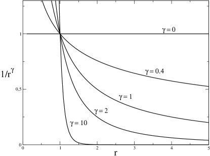
Figure 1: A graph that represents the intensity of the interactions between two individuals as a function of the distance $r$, according to some values of $\gamma$. As $\gamma$ (the exponent decay) increases, the interaction range decreases. When $\gamma=0$, the interaction range is infinity; that is, the intensity of the interaction does not depend on the distance.

The update of the population must obey the rule $N(t+\leavevmode\nobreak\ \Delta t)=N(t)+\leavevmode\nobreak\ \Delta t\sum_{i=1}^{N}R_{i}$. In the limit $\Delta t\to 0$, one has the differential equation $dN/dt=\sum_{i=1}^{N}R_{i}$. By equation (2), one has

$$\frac{d}{dt}N=\sum_{i=1}^{N}\left(k_{i}-J_{1}I_{i}^{(1)}+J_{2}I_{i}^{(2)}\right),$$ (3)

where

$$I_{i}^{(l)}\equiv\sum_{j\neq i}\frac{1}{|\mathbf{r}_{i}-\mathbf{r}_{j}|^{\gamma_{l}}}$$ (4)

is the (cooperative or competitive) interaction term that individual $i$ feels from its neighbors.

In appendix (B), a extended version of the calculus of Mombach et all with respect to the sum in equation (4) is presented. One can prove (see the appendix) that the interaction factor $I_{i}^{(l)}$ is the same for all individuals of the population (regardless of $i$), and it has the form

$$I^{(l)}\equiv I_{i}^{(l)}=\frac{\omega_{D}}{D_{f}(1-\frac{\gamma_{l}}{D_{f}})}\left[\left(\frac{D_{f}}{\omega_{D}}N\right)^{1-\frac{\gamma_{l}}{D_{f}}}-1\right].$$ (5)

Here, $\omega_{D}$ is a constant that depends exclusively on the Euclidean dimension $D(=1,2,3)$ in which the population is embedded, and $D_{f}$ is the fractal dimension of the spatial structure formed by the population. To maintain the physical propert that $I_{i}^{(l)}$ is positive (note that the sum in equation (4) is over absolute terms), the model must be restricted to the case where $\omega_{D}/D_{f}<N$. In fact, it is demonstrated in the analysis around equation (40) (appendix B), that $\omega_{D}/D_{f}\sim 1$ (which is much smaller than the population size).

As presented in fabiano-pre , one can write the term on the right-hand side of expression (5) by means of the generalized logarithm (see appendix (A)):

$$I^{(l)}=\frac{\omega_{D}}{D_{f}}\ln_{\tilde{q}_{l}}\left(\frac{D_{f}}{\omega_{D}}N\right),$$ (6)

where

$$\tilde{q}_{l}\equiv 1-\gamma_{l}/D_{f}.$$ (7)

The parameter $q_{l}$ gives information about the relation between the decay exponent and the fractal dimension of the population.

By introducing the average of the intrinsic growth rate $\langle k\rangle\equiv(1/N)\sum_{i=1}^{N}k_{i}$, employing the definition $J_{l}^{\prime}\equiv J_{l}\omega_{D}/D_{f}$, and using result (6), one obtain from (3) the Richard-like model

$$G(N)=\frac{1}{N}\frac{d}{dt}N=\langle k\rangle-J_{1}^{\prime}\ln_{\tilde{q_{1}}}\left(\frac{D_{f}}{\omega_{D}}N\right)+J_{2}^{\prime}\ln_{\tilde{q_{2}}}\left(\frac{D_{f}}{\omega_{D}}N\right).$$ (8)

The per- capita growth rate $G(N)$ gives information about the type of interaction that predominates in the population. For instance, $dG(N)/dN>0$ means that cooperation predominates: the larger the population is, the larger the per- capita growth rate is. However, $dG(N)/dN<0$ means that competition predominates: the larger the population is, the smaller the per- capita growth rate is.

Comments

The result (8) depends only on the macroscopic parameters of the system, besides to be deduced from microscopic (or individual level) premises. That is a remarkable result, and it was first obtained by Mombach et all in the context of inhibitory interactions and is now expanded to cooperative interactions. This result represents a significant advance in the knowledge of patterns in population growth. It is because the model is not a phenomenological one, that is, it is not a model that is constructed to fit macroscopic data. The MLBI model, which was extended here, is deduced from the own individuals’ interactions. Then, the macroscopic behavior emerges as a consequence of the interactions.

Moreover, the model presented in this work is more robust than its original version. The original model is fully obtained by assuming that $J^{\prime}_{2}=0$ in (8). In this case, the per- capita growth rate $G(N)$ is a monotonically decreasing function of the size of the population (because if $J^{\prime}_{2}=0$, then $dG/dN<0$ for any population size). Consequently, the simpler form of expression (8), which does not present the cooperative effects, cannot explain the Allee effect. However, if the cooperative term is considered ($J^{\prime}_{2}\neq 0$ in (8)), the Allee effect can be predicted by the model. This effect will be discussed in more detail in the next section.

III The Allee Effect

The Allee effect is the property of some populations to increase their per- capita growth rates with incriasing population size when the population is small allee_revisao ; theta-logistic . For instance, in figure (3), the experimental data of the per- capita growth rate of the muskox population are presented as a function of the population size. For a small population the experimental data show an increasing trend with respect to the size of the population. Then, when the population is sufficiently large, the per- capita growth rate decreases.

This effect has been studied in recent theoretical models theta-logistic ; courchamp1999 ; alexandre_allee . However, these models are restricted to the macroscopic approach and do not consider the microscopic level of the system. In the model proposed here, the Allee effect can not only be obtained, but it can also be interpreted as a macroscopic behavior that is observed as a consequence of the interactions of the individuals that compose the population.

To show that model (8) can present the Allee effect, figure (2) is included. The lower graph of this figure presents the form of $G(N)$ when $J_{2}^{\prime}>J_{1}^{\prime}$ and $\tilde{q}_{1}>\tilde{q}_{2}$. In this specific case, the per- capita growth rate reaches its maximum at $N=N^{*}$. This result can be explained by analyzing the two terms that composed $G(N)$ in equation (8). The upper graphic of this figure presents the curves $\langle k\rangle+J_{2}^{\prime}\ln_{\tilde{q_{2}}}\left(\frac{D_{f}}{\omega_{D}}N\right)$ (the intrinsic reproductive rate and cooperative term) and $J_{1}^{\prime}\ln_{\tilde{q_{1}}}\left(\frac{D_{f}}{\omega_{D}}N\right)$ (the competitive term) as a function of $N$. The two curves are monotonic crescent functions of $N$, but they have different forms. The per- capita growth rate $G(N)$ is the difference between these two functions. For small $N$, $G(N)$ is an increasing function of the population size; that is the Allee effect.

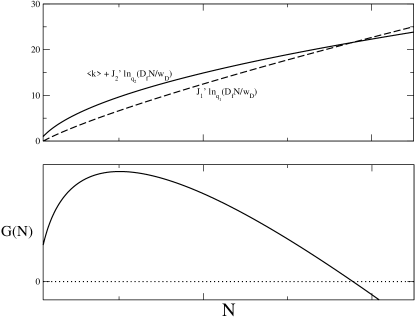
Figure 2: The upper graph presents separately the functions that compos $G(N)$ as a function of $N$, which conform to equation (8): $\langle k\rangle+J_{2}^{\prime}\ln_{\tilde{q_{2}}}\left(\frac{D_{f}}{\omega_{D}}N\right)$ (the intrinsic reproductive rate and cooperative term); and $J_{1}^{\prime}\ln_{\tilde{q_{1}}}\left(\frac{D_{f}}{\omega_{D}}N\right)$ (the competitive term). In this particular case, it was assumed $J_{2}^{\prime}>J_{1}^{\prime}$ and $q_{1}>q_{2}$. The lower graph presents $G(N)$ (which is obtained by the difference between the above two functions) as a function of $N$.

One can find the population size $N^{*}$ at which $G$ is at its maximum by taking $dG(N)/dN=\leavevmode\nobreak\ 0$ in (8), which gives

$$N^{*}=\frac{\omega_{D}}{D_{f}}\left(\frac{J_{2}}{J_{1}}\right)^{\frac{1}{\tilde{q}_{1}-\tilde{q}_{2}}}.$$ (9)

Note that if $J_{2}=0$, which is the MLBI model, then $N^{*}$ is null or indeterminate. That is, the MLBI model cannot explain Allee effect.

One can also find when $G(N)$ becomes null, which happens at the the threshold value $N=N_{c}$ in which the per capita growth rate became null, that is, $G(N_{c})=0$. This threshold population value can be determined by solving the transcendental equation

$$N_{c}=\frac{\omega_{D}}{D_{f}}e_{q_{1}}\left[\frac{\langle k\rangle}{J_{1}^{\prime}}\ln_{q_{2}}\left(\frac{D_{f}}{\omega_{D}}N_{c}\right)\right].$$ (10)

When $N>N_{c}$, the population is decreasing. Note that the maximum value of $G$ happens when the difference between the two functions plotted in the upper graph of figure (2) is maximal, and the threshold value $N_{c}$ happens when these two functions are equal.

Model (8) fits very well to the muskox population data, which are presented in figure (3). According to the model and result (9), the transition from cooperation to competition for the muskox data is $\leavevmode\nobreak\ N^{*}\approx 246$.

Figure 3: The experimental data of the per- capita growth rate of a population of muskoxen as a function of the population size. The data were obtained directly from gregory . The line is the fit from model (8) with the following parameters: $J_{1}^{\prime}\approx 1.0305$; $J_{2}^{\prime}\approx 1.0327$; $q_{1}\approx 0.9859$; $q_{2}\approx 0.9855$; and $\langle k\rangle\approx 6.828$. The term $D_{f}/\omega\equiv 1$ was kept fixed. The statistical analysis shows $R^{2}=0.10694$.

III.1 Comments

One can interpret the Allee effect as cooperative and competitive interactions between the individuals of the population. When the population is too small, cooperation predominates, which favors the increase of the per- capita growth rate as $N$ increases. However, when the population is sufficiently large, competition predominates, which implies a decrease in the population growth rate as the population increases.

With respect to the spatial structure of the population and its representation by the model presented here, a good example is pollination in plants. The smaller the inter-individual distance is , the greater the efficiency of the pollination is allee_revisao ; allee_ghazoul ; allee_desert_mustard ; allee_annual_plant . As result, there is a cooperative effect (or facilitation, as argued in allee_1949 ) that is strongly dependent on the distance between the individuals. However, when the inter-individual distance is small, competitive effects begin to appear in form of sunlight disputes, elimination of inhibitory toxins, or competition for soil or other resources. In this way, there is a tradeoff between the individuals to stay close or more distant. The Allee effect is an example of an emergent phenomenon that can emerge as a consequence of these types of individual-individual mechanisms.

IV Analysis of a Special Case: $\gamma\equiv\gamma_{1}=\gamma_{2}$

This section will be restricted to the special case in which the two decay exponents (for competition and cooperation) have equal values. That is, $\gamma\equiv\gamma_{1}=\gamma_{2}$, which is equivalent to saying that $\tilde{q}\equiv\tilde{q}_{1}=\tilde{q}_{2}$. In this particular case, model (8) becomes

$$\frac{1}{N}\frac{dN}{dt}=\langle k\rangle+J^{\prime}\ln_{\tilde{q}}\left(\frac{D_{f}}{\omega_{D}}N\right),$$ (11)

where it is assumed $J^{\prime}\equiv J_{2}^{\prime}-J_{1}^{\prime}$. The parameter $J^{\prime}$, which can assume both positive and negative values, determines what type of interaction has more strength: cooperation ($J^{\prime}>0$) or competition ($J^{\prime}<0$). When $\tilde{q}=0$, i.e. when $\gamma=D_{f}$, the generalized logarithm function becomes the usual logarithm, and then, Eq. (11) is the Gompertz growth model.

Using the properties of the generalized logarithm, one can show that equation (11) can be rewritten as

$$\frac{d}{dt}N=aN^{1+q}-bN.$$ (12)

with solution

$$N(t)=\left[\frac{a}{b}+\left(N_{0}^{-q}-\frac{a}{b}\right)e^{bqt}\right]^{-\frac{1}{q}}.$$ (13)

In the last two equations, the parameters $a$ and $b$ are given by

$$a\equiv\frac{J^{\prime}}{\tilde{q}}\left(\frac{D_{f}}{\omega_{D}}\right)^{\tilde{q}},$$ (14)

and

$$b\equiv\frac{J^{\prime}}{\tilde{q}}-\langle k\rangle,$$ (15)

respectively. Model (12) is the Richards model richards_59 , which is utilized in bertalanffy-model ; savageau-1979 ; west-nature to describe animal growth. Recently, this model was studied by West et al in the context of the growth of cities west-pnas . Thus, the Richards model is the same model that was deduced here from the individuals’ interactions.

The sign of the argument of the exponential in (13) is important, as it determines the convergence (or divergence) of the population. When $b\tilde{q}<0$, the exponential term goes to zero at $t\to\infty$, and then, the population has a saturation. However, when $b\tilde{q}>0$ the exponential diverges. Thus, there is a change in the behavior when $b\tilde{q}=0$, which happens when $\gamma=\gamma^{*}$, where

$$\gamma^{*}\equiv D_{f}\left(1-\frac{J^{\prime}}{\langle k\rangle}\right)$$ (16)

(according to the definitions in (15) and (7)).

The term $\gamma^{*}$ plays an important role in the analysis of the population growth behavior, and it will be discussed in more detail in the next section. The sign of the exponent $(-1/\tilde{q})$ in (13) is also important in the analysis of the dynamics. Transition behavior happens when $1/\tilde{q}=0$, that is, when $\gamma=D_{f}$ (according to (7)). In the next section, the analysis of solution (13) for the predomination of cooperation and competition will be presented separately. The convergence or divergence of the population according to the value of $\gamma$ will also be analyzed there.

IV.1 The Predominance of Cooperation

Let’s analyze the particular case in which the system described by model (11) presents cooperation predominance, that is, when $J^{\prime}>0$. In this case, given that $\langle k\rangle$ is positive, the population always grows, without saturation. However, the way the population grows depends on the value of the exponent decay.

For instance, when $\gamma>D_{f}$, then $b<0$, $-1/\tilde{q}>0$ and $b\tilde{q}>0$. The solution for this case (see (13)) can be written as

$$N(t\gg 1)\sim\left[e^{b\tilde{q}t}\right]^{-\frac{1}{\tilde{q}}}=e^{\left(\langle k\rangle-\frac{J^{\prime}}{\tilde{q}}\right)t}.$$ (17)

That is, $\gamma>D_{f}$ implies exponential growth of the population, which is the Malthus model with growth rate $-b=\langle k\rangle-\frac{J^{\prime}}{\tilde{q}}$ (see Eq (15)). When $\gamma=D_{f}$ (the Gompertz model), the population diverges asymptotically as $N(t\gg 1)\sim e^{e^{J^{\prime}\frac{\omega_{D}}{D_{f}}t}}$. When $\gamma<D_{f}$, the population diverges at a finite time $t_{c}$ given by

$$t_{c}\equiv\frac{-1}{b\tilde{q}\ln\left(1-\frac{b}{a}N_{0}^{-\tilde{q}}\right)}.$$ (18)

These results are summarized in figure (4).

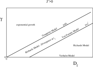
Figure 4: A schema of the population growth according to the exponent decay $\gamma$ when cooperation predominates ($J^{\prime}>0$). The upper graph is the phase diagram corresponding to $\gamma$-x-$D_{f}$; the lower graph presents the population growth behavior as a function of $\gamma$, where $D_{f}$ is fixed. The exponent decay represents the following models: $\gamma=0$ implies that one has the Verhulst model; $\gamma=\gamma^{*}$ implies one has Von Foerster model; $\gamma=D_{f}$ implies one has the Gompertz model. When $\gamma<D_{f}$, one has the Richards model, and hence, the population diverges at a finite time $t_{c}$ given by (18). When $\gamma=D_{f}$ (the Gompertz model), the population diverges as $t\to\infty$. lastly, when $\gamma>D_{f}$, the population grows exponentially (the Malthus model), as in Eq. (17).

IV.2 The Predominance of Competition

When competition predominates, that is, when $J^{\prime}<0$, the model described here is quite similar to the MLBI model. Thus, the analysis of the convergence or divergence of the population is similar to the analysis discussed and presented by D’Onofrio in donofrio .

When $\gamma<\gamma^{*}$, which implies $-1/q>0$ and
$bq<0$, solution (13) implies that the population converges to a finite size - which is the carrying capacity - and is given by

$$K=\left(\frac{a}{b}\right)^{-\frac{1}{\tilde{q}}}=\left[\frac{\left(\frac{D_{f}}{\omega_{D}}\right)^{\tilde{q}}}{1-\langle k\rangle\frac{\tilde{q}}{J^{\prime}}}\right]^{-\frac{1}{\tilde{q}}}.$$ (19)

When $\gamma>\gamma^{*}$ (which implies $\tilde{q}<0$), at $t\gg 1$ solution (13) becomes

$$N(t)\sim e^{\left(\langle k\rangle-\frac{J^{\prime}}{\tilde{q}}\right)t}=e^{\left(\langle k\rangle-|\frac{J^{\prime}}{\tilde{q}}|\right)t},$$ (20)

i.e., one has exponential growth (the Malthus model). When $|J^{\prime}/\tilde{q}|<\langle k\rangle$ the population diverges exponentially. As the population grows indefinitely even due to predominance of competition, one can call this situation weak competition. However, when $|J^{\prime}/\tilde{q}|>\langle k\rangle$, the population decays exponentially, and it goes to extinction for $t\to\infty$. Thus, one can call this situation strong competition. These results are summarized in figure (5). The case $\gamma=\gamma^{*}$ will be analyzed in the next section in the general context of the parameter $J^{\prime}$ (which may be positive or negative).

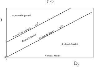
Figure 5: A schema of the population growth according to the exponent decay $\gamma$, when competition predominates ($J^{\prime}<0$). whereas the upper graph is the phase diagram $\gamma$-x-$D_{f}$, the lower graph presents the population growth behavior as a function of $\gamma$, where $D_{f}$ is fixed. The exponent decay represents the following models: $\gamma=0$ implies one has the Verhulst model; $\gamma=\gamma^{*}$ implies power law growth (see eq. (23)); $\gamma=D_{f}$ implies one has the Gompertz model. When $\gamma<\gamma^{*}$, the population converges to a finite size (the carrying capacity $K$), which is given by (19). When $\gamma>\gamma^{*}$ the population presents exponential growth, which conforms to eq. (20), and the population goes to extinction when $|J^{\prime}/\tilde{q}|>\langle k\rangle$; it diverges otherwise.

IV.3 Comments about $\gamma=\gamma*$ and the Human Population Growth

The particular case that $\gamma=\gamma^{*}$ must receive more attention. In this case, the parameter $b$ becomes null (according to Eq. (16) and (15)), and then, the model (13) becomes

$$\frac{d}{dt}N=aN^{1+\tilde{q}}.$$ (21)

This is the von Foerster growth model, which was studied both in von-foester and more recently in polones to describe human population growth. The solution of model (21) is

$$N(t)=N_{0}e_{\tilde{q}}\left(\frac{a}{N_{0}^{\tilde{q}}}t\right),$$ (22)

which was presented in fabiano-physicaA ; fabiano-pre , where $e_{q}(x)$ is the generalized exponential function (see appendix A). Note that result (22) is exactly the model proposed in polones_q . In this reference, the model was introduced by a modification of the exponential term of the Malthus model solution without any justification. However, with the formulation of the microscopic model proposed here, all of the involved quantities have a physical interpretation, and the growth behavior described by (22) is a consequence of the of interactions of the individuals.

Given that $\omega_{D}$, $D_{f}$, and $\langle k\rangle$ are positive parameters, the manner in which the population grows for large $t$ is totally dependent on $J^{\prime}$. For instance, when $J^{\prime}=0$, the population grows exponentially because the competitive and cooperative strength completely cancel each other out, and then, the population grows without individual interactions.

When $J^{\prime}<0$, solution (22) behaves asymptomatically as a power law:

$$N(t\gg 1)\sim t^{-\frac{\langle k\rangle}{J^{\prime}}}.$$ (23)

In this way, if $J^{\prime}<0$, then the population diverges only when $t\to\infty$. The concavity of $N(t)$ is also determinede by $J^{\prime}$: if $J^{\prime}>-\langle k\rangle$, then $N(t)$ is a convex function, and it is concave otherwise. Whereas $J^{\prime}<0$ the population diverges only when $t\to\infty$, for $J^{\prime}>0$ the population diverges at a finite time $t_{c}$, which is given by

$$t_{c}=\frac{1}{J^{\prime}}\left(\frac{N_{0}D_{f}}{\omega_{D}}\right)^{-\frac{J^{\prime}}{\langle k\rangle}}.$$ (24)

Figure (6) summarizes these conclusions.

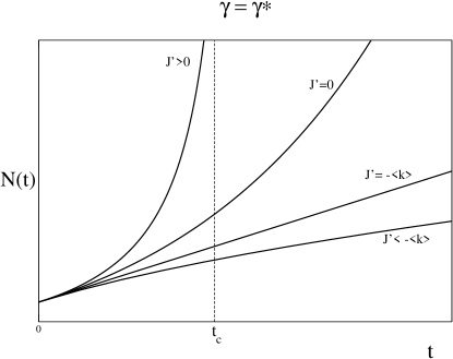
Figure 6: The time evolution of the population according to the strength of the interaction $J^{\prime}$ for $\gamma=\gamma^{*}$. When $J^{\prime}>0$, that is, when one has cooperation, the population diverges at a finite time $t_{c}$ (in the Von Foerster model). When $J^{\prime}=0$, the population experiences exponential growth. In this case, the interaction effect is fully nullified and the growth rate is given only by the intrinsic growth rate $\langle k\rangle$. When $J^{\prime}<0$, that is, when one has competition, the population diverges only as $t\to\infty$. The special cases are: $J^{\prime}=-\langle k\rangle$, linear growth; and $J^{\prime}<-\langle k\rangle$, logarithmic growth. $N(t)$ is a convex function when $J^{\prime}>-\langle k\rangle$, and it is a concave function otherwise.

When $J^{\prime}>0$, it is interesting to write solution (21) in terms of the critical time $t_{c}$ in which the population diverges.Thus, solution (22) behaves as

$$N(t)\sim(t_{c}-t)^{-\frac{\langle k\rangle}{J^{\prime}}}$$ (25)

when cooperation predominates. An interesting application of this result is in human population growth, as represented in figure (7). Note that Eq. (25) applies very well to human population growth, as the data from $1000$ A.D. until $2013$ conform with what was presented in polones ; von-foester . However, with the presentation of the microscopic point of view of the interactions between the individuals, one can argue that the “divergent behavior” of the human population can be seen as a result of cooperative effects, as the parameter $J^{\prime}$ must be positive (i.e. cooperation predominates) to fit the data.

Figure 7: The human population as a function of time since the Middle Ages. The data were obtained from polones and from the U.S. Census Bureau census . The curve is a plot of the equation $N(t)=65,6(2026-t)^{-0,78}$ (from Eq. (25)), whose parameters values were obtained via a data fit.

V Conclusion

In the present work, one has proposed a growth model based on the microscopic level of the interaction of the individuals that constitute the population. It was shown that the model reached several well known growth models presented in literature as special cases. For instance, one has obtained the Malthus, Verhulst, Gompertz, Richards, Bertalanffy, power law, and Von Foerster growth models. The present model explains some macroscopic behaviors using a non- phenomenological approach. Moreover, it uses parameters that have physical meanings and that can be measured in real systems. In addiction, the model showed more flexibility than the original version (i.e., the MLBI model). For instance, the extended model presented here permits us to explain the Allee effect as an emergent behavior from the individual-individual interactions, which is contrast to the common phenomenological explanation presented in the literature. It is important to stress that the MLBI model, which considers only competitive interactions, can not explain this effect.

It was observed that the relation between the decay exponent ($\gamma$), the fractal dimension ($D_{f}$) of the population, and the interaction strength ($J$) determine the behavior of the population growth. For instance, one has presented a phase diagram in which one related diverse types of growth as consequences of the distance dependent interactions (by the exponent decay $\gamma$) and the fractal dimension of the population. Moreover, one has shown how the strength of the interaction gives both the concavity of the growth (as a function of time) and the saturation or divergence of the population.

In conclusion, the model proposed here incorporates many types of macroscopic ecological patterns by focusing on the balance of cooperative and competitive interactions at the individual level. In this way, the model presents a new direction in the search for universal patterns, which could shed more light on population growth behavior.

Appendix A The Generalized Logarithm and Exponential Function

In this appendix, one presents the generalizations of the logarithmic and exponential functions and some of their properties. The introduction of the functions is shown to be very useful for dealing with the mathematical representation of the population growth model that is presented in this work.

The $\tilde{q}$-logarithm function is defined as

$$\ln_{\tilde{q}}(x)=\lim_{\tilde{q}^{\prime}\rightarrow\tilde{q}}\frac{x^{\tilde{q}^{\prime}}-1}{\tilde{q}^{\prime}}=\int_{1}^{x}\frac{dt}{t^{1-\tilde{q}}}\;,$$ (26)

which is the area of the crooked hyperbole, and is controlled by $\tilde{q}$. This equation is a generalization of the natural logarithm function, which is reproduced when $\tilde{q}=0$. This function was introduced in the context of nonextensive statistical mechanics tsallis_1988 ; tsallis_qm and was studied recently in arruda_2008 ; martinez:2008b ; Martinez:2009p1410 . Some of the properties of this function are as follows: for $\tilde{q}<0$, $\ln_{\tilde{q}}(\infty)=-1/\tilde{q}$; for $\tilde{q}>0$, $\ln_{\tilde{q}}(0)=-1/\tilde{q}$; for all $\tilde{q}$, $\ln_{\tilde{q}}(1)=0$; $\ln_{\tilde{q}}(x^{-1})=-\ln_{-\tilde{q}}(x)$; $d\ln_{\tilde{q}}(x)/dx=x^{\tilde{q}-1}$. Moreover, the $\tilde{q}$-logarithm is a function: convex for $\tilde{q}>1$; linear for $\tilde{q}=1$; and concave for $\tilde{q}<1$.

The inverse of the $\tilde{q}$-logarithm function is the $\tilde{q}$-exponential function, which is by

$$e_{\tilde{q}}(x)=\left\{\begin{array}[]{ll}\lim_{\tilde{q}^{{}^{\prime}}\to\tilde{q}}(1+\tilde{q}^{{}^{\prime}}x)^{\frac{1}{\tilde{q}^{{}^{\prime}}}}&,\textrm{ if $\tilde{q}x>-1$}\\ 0&,\textrm{ otherwise}\end{array}\right.\;.$$ (27)

Some properties of this function are as follows: $e_{\tilde{q}}(0)=1$, for all $\tilde{q}$; $\left[e_{\tilde{q}}(x)\right]^{a}=e_{\tilde{q}/a}(ax)$, where $a$ is a constant; and for $a=-1$, one has $1/e_{\tilde{q}}(x)=e_{-\tilde{q}}(-x)$. Moreover, the $\tilde{q}$-exponential is a function: convex for $\tilde{q}<1$; linear for $\tilde{q}=1$; and concave for $\tilde{q}>1$.

Appendix B A Detailed Calculus of $I_{i}^{(l)}$

In this appendix one presents a detailed calculus for the intensity of the interaction felt by a single individual $i$ from the other individuals of the population, which is represented by $I_{i}^{(l)}$ (see section (II). One follows Mombach et al mombach to show that this intensity is independent of the individual. That is, it is the same for all individuals of the population and depends only on the size of the population. More specifically, one shows that $I_{i}^{(l)}=I^{(l)}(N)$ regardless of $i$.

First, it was presented in section (II) that

$$I_{i}^{(l)}=\sum_{j\neq i}\frac{1}{|\mathbf{r}_{i}-\mathbf{r}_{j}|^{-\gamma_{l}}}=\sum_{j=1}^{N}\frac{\left(1-\delta_{ij}\right)}{|\mathbf{r}_{i}-\mathbf{r}_{j}|^{-\gamma_{l}}},$$ (28)

where $\delta_{ij}$, which is the Kronecker’s delta, was introduced to avoid the restriction in the sum. Introducing the property

$$f(\mathbf{r}_{0})=\int_{V_{D}}d^{D}\mathbf{r}\delta(\mathbf{r}-\mathbf{r}_{0})f(\mathbf{r}),$$ (29)

where $\delta(\cdots)$ is the Dirac’s delta, the expression (28) becames

$$I_{i}^{(l)}=\sum_{j=1}^{N}(1-\delta_{ij})\int_{V_{D}}d^{D}\mathbf{r}\delta\Big{(}\mathbf{r}-(\mathbf{r}_{j}-\mathbf{r}_{i})\Big{)}|\mathbf{r}|^{-\gamma_{l}}.$$ (30)

In the last two expressions, was introduced: $D(=1,2,3)$, which is the Euclidean dimension in which the population is embedded, and $V_{D}$, which is the total (hipper)volume (in $D$ dimensions) that contains the population. The form represented in (30) was obtained by the variable substitution $\mathbf{r}_{j}-\mathbf{r}_{i}$ by $\mathbf{r}$, using Dirac’s delta.

Some algebraic manipulation and the introduction of $r\equiv|\mathbf{r}|$, allows to write

$$I_{i}^{(l)}=\int_{V_{D}}\frac{d^{D}\mathbf{r}}{\mathbf{r}^{\gamma_{l}}}\sum_{j\neq i}\delta\Big{(}\mathbf{r}-(\mathbf{r}_{j}-\mathbf{r}_{j})\Big{)}.$$ (31)

Note that $dN(\mathbf{r})\equiv d^{D}\mathbf{r}\sum_{j\neq i}\delta\Big{(}\mathbf{r}-(\mathbf{r}_{j}-\mathbf{r}_{j})\Big{)}$ is the number of individuals which is at the element of (hipper)volume $d^{D}\mathbf{r}$ at the distance $\mathbf{r}$ from the individual $i$, localized at $\mathbf{r}_{i}$. In this way, the density of individuals at $\mathbf{r}_{i}+\mathbf{r}$ (neighbors of $i$), that is $\rho(\mathbf{r}_{i}\leavevmode\nobreak\ +\leavevmode\nobreak\ \mathbf{r})=dN(\mathbf{r})/d^{D}\mathbf{r}$, can be written as

$$\rho(\mathbf{r}_{i}+\mathbf{r})=\sum_{j\neq i}\delta\Big{(}\mathbf{r}-(\mathbf{r}_{j}-\mathbf{r}_{j})\Big{)}.$$ (32)

The density of individuals can also be thought of in terms of the scale of the system (in conformity with Falconer ). The volume of the system grows in the form $V_{D}\sim L^{D}$, where $L$ is the typical size of the system. However, the number of individuals grows as the form $N\sim L^{D_{f}}$, where $D_{f}$ is the fractal dimension formed by the spatial structure of the population. By considering $r$, which is the absolute distance from $i$, as a typical distance of the system, one can say that the density of individuals ($V_{D}/N$) has the form

$$\rho(\mathbf{r}_{i}+\mathbf{r})\equiv\rho(r)=a\frac{r^{D_{f}}}{r^{D}},$$ (33)

where $a$ is a constant.

Using results (33) and (32) in (31), one obtains

$$I_{i}^{(l)}=a\int_{V_{D}}d^{D}\mathbf{r}r^{D_{f}-D-\gamma_{l}}.$$ (34)

Note that the integration argument does not depend on the angular coordinates. Thus, one can write $d^{D}\mathbf{r}=\leavevmode\nobreak\ r^{D-1}drd\Omega_{D}$, where $d\Omega_{D}$ is the solid angle, which implies

$$I_{i}^{(l)}=a\int d\Omega_{D}\int_{r_{0}}^{R_{max}}drr^{D_{f}-1-\gamma_{l}}$$ (35)

Note that the only term that depends on the Euclidean dimension is the solid angle, and the integral $\int d\omega_{D}$ assumes the following values according to these tree possibilities: $D=1$, $\int d\omega_{1}=1$; $D=2$, $\int d\Omega_{2}=2\pi$; $D=3$, $\int d\Omega_{3}=4\pi$. By introducing the constant $\omega_{D}=a\int d\Omega_{D}$, which depends only on $D$, one obtains

$$I^{(l)}\equiv I_{i}^{(l)}=\omega_{D}\left(\frac{R_{max}^{D_{f}-\gamma_{l}}-1}{D_{f}-\gamma_{l}}\right)$$ (36)

Thus, $I_{i}^{(l)}$ does not depend on the label $i$ anymore. As a result, one can say that $I_{i}^{(l)}=I^{(l)}$ regardless of $i$.

Furthemore, one can introduce the total number of individuals in the relation above by the following thinking. The total number of individuals in the population can be determined by the integral

$$N=\int dN(r)=\int_{V_{D}}d^{D}\mathbf{r}\rho(r).$$ (37)

Using equation (33) and integrating the solid angle, one obtains

$$N = \omega_{D}\int_{0}^{R_{max}}r^{D_{f}-1}dr$$ (38)

$$= \omega_{D}\int_{0}^{r_{0}}r^{D_{f}-1}+\omega_{D}\int_{r_{0}}^{R_{max}}r^{D_{f}-1}$$ (39)

$$= \omega_{D}\frac{r_{0}^{D_{f}}}{D_{f}}+\omega_{D}\frac{R_{max}^{D_{f}}}{D_{f}}-\omega_{D}\frac{r_{0}^{D_{f}}}{D_{f}}.$$ (40)

Note that the first term on the right in (39) and (40) can be zero (indicating the absence of individuals) or 1 (indicating the presence of a single individual). These values are possible because the ratio of the individual is $r_{0}$, and hence, there can be at most one individual inside the region that consists of the length between $0$ and $r_{0}$. Thus, for $r_{0}=1$, $\omega_{d}/D_{f}\sim 1$. $R_{max}$ can be obtained from (40), which is a function of $N$ according to

$$R_{max}=\left(\frac{D_{f}}{\omega_{D}}N\right)^{\frac{1}{D_{f}}}.$$ (41)

Returning to relation (36) one finds

$$I=I(N)=\frac{\omega_{D}}{D_{f}(1-\frac{\gamma}{D_{f}})}\left[\left(\frac{D_{f}}{\omega_{D}}N\right)^{1-\frac{\gamma}{D_{f}}}-1\right].$$ (42)

By introducing $\tilde{q}=1-\gamma/D_{f}$ and the properties of the generalized logarithm (Appendix A) one obtains

$$I=I(N|D,\tilde{q})=\frac{\omega_{D}}{D_{f}}\ln_{\tilde{q}}\left(\frac{D_{f}}{\omega_{D}}N\right).$$ (43)

References

J. D. Murray. Mathematical biology I: an introduction. Springer, New York (2002).

Sorin Solomon. Generalized Lotka-Volterra (GLV) Models and Generic Emergence of Scaling Laws in Stock Markets. arXiv:cond-mat/9901250

Dominik Strzalka. Connections Between Von Foester Coalition Growth Model and Tsallis q-Exponential. Acta Physica Polonica B No 1, Vol. 40 (2009).

Timothy A. Kohler, George G. Gumerman. Dynamics in Human and Primate Societies. Oxford University Press, USA (2000).

Marvin Chester. A Law of Nature? Open Journal of Ecology Vol.1, No.3, 77-84 (2011)

Guiot C, Degiorgis PG, Delsanto PP, Gabriele P, Deisboeck TS. Does tumor growth follow a ”universal law”? J Theor Biol. 2003 Nov 21;225(2):147-51.

Geoffrey B. West, James H. Brown & Brian J. Enquist. A general model for ontogenetic growth. NATURE VOL 413 (2001).

Luis M. A. Bettencourt et all. Growth, innovation, scaling, and the pace of life in cities. PNAS April 24, vol. 104 no. 17 (2007).

Christian Kuehn, Stefan Siegmund, Thilo Gross. On the dynamical analysis of evolution equations via generalized models. http://arxiv.org/abs/1012.4340

Brenno Caetano Troca Cabella, Alexandre Souto Martinez and Fabiano Ribeiro. Data collapse, scaling functions, and analytical solutions of generalized growth models. PHYSICAL REVIEW E 83, 061902 (2011).

Brenno Caetano Troca Cabella, Fabiano Ribeiro, Alexandre Souto Martinez. Effective carrying capacity and analytical solution of a particular case of the Richards-like two-species population dynamics model. Physica A 391 (2012) 1281-1286.

Fabiano Ribeiro, Brenno Caetano Troca Cabella and Alexandre Souto Martinez. Richards-like two species population dynamics model. Paper submited to the Physical Review E.

L. Barberis, C.A. Condat, P. Román.Vector growth universalities. Chaos, Solitons & Fractals 44 (2011) 1100-1105.

Malthus, T. R.. An Essay on the Principle of Population as It Afects the Future Improvement of Society. J. Johnson, London, 1798.

Leah Edelstein-Keshet. Mathematical Models in Biology (Classics in Applied Mathematics. SIAM: Society for Industrial and Applied Mathematics; 1 edition (February 2005).

Verhulst, P.F., Recherches mathematiques sur la loi d’accroissement de la population. Nouveaux Memoires de l’Academie Royale des Sciences et Belles-Lettres de Bruxelles 18 (1845) 1-38.

Verhulst, P.F.. Deuxieme memoire sur la loi d’accroissement de la pop- ulation. Nouveaux memoires de l’Academie Royale des Sciences et Belles Lettres de Bruxelles, 20 (1847) 1-32.

Gompertz, R.. On the Nature of the Function Expressive of the Law of Human Mortality, and on a New Mode of Determining the Value of Life Contingencies. Philos. Trans. R. Soc. London, 115 (1825) 513-585.

Haybittle JL. The use of the Gompertz function to relate changes in life expectancy to the standardized mortality ratio. Int J Epidemiol. 1998 Oct;27(5):885-9.

Marcel Ausloos Another analytic view about quantifying social forces. arXiv:1208.6179, Submitted on 30 Aug 2012.

. Richards F., J. Exp. Bot., 10 (1959) 290.

A. Gregorczyk. Richards Plant Growth Model. Journal of Agronomy and Crop Science, Volume 181, Issue 4, pages 243-247 (1998).

L. von Bertalanffy. Quantitative laws in metabolism and growth. Q Rev Biol. 1957 Sep;32(3):217-31.

L. von Bertalanffy. Principles and theory of growth, in Fundamental Aspects of Normal and Malignant Growth. (W. W. Nowinski Ed.), Elsevier, New York, 1960, pp. 137-259.

MICHAEL A. SAVAGEAU. Growth Equations: A General Equation and a Survey of Special Cases. MATHEMATICAL BIOSCIENCES 48:267-278(1980).

Strzalka, Dominik; Grabowski, Franciszek. Towards possible q-generalizations of the Malthus and Verhulst growth models. Physica A, Volume 387, Issue 11, p. 2511-2518.

Ginzburg, L.R.. The analogies of the “free motion” and “force” concepts in population theory. Ratner, V.A. Ed., Studies on theoretical genetics, Academy of Sciences of the USSR, Novosibirsk, 65-85(1972).

. J. M. Yeomans. Statistical Mechanics of Phase Transitions. Oxford University Press, USA (June 25, 1992).

Leo P. Kadanoff. Statistical Physics: Statics, Dynamics and Remormalization. World Scientific Pub Co Inc (July 2000).

. Nino Boccara. Modeling Complex Systems (Graduate Texts in Contemporary Physics). Springer; 1 edition (November 18, 2003).

Melanie Mitchell. Complexity: A Guided Tour. Oxford University Press, USA (September 1, 2011).

J. C. M. Mombach, N. Lemke, B. E. J. Bodmann and M. A. P. Idiart.A mean-field theory of cellular growth. Europhys. Lett., 59 (6), pp. 923-928 (2002).

d’Onofrio A. textitFractal growth of tumors and other cellular populations: Linking the …. Chaos, Solitons & Fractals (2008), doi:10.1016/j.chaos.2008.04.014.

Webpage: http://www.census.gov/population/international/index.html

Richard M. Sibly, Daniel Barker, Michael C. Denham, Jim Hone, Mark Pagel. On the Regulation of Populations of Mammals, Birds, Fish, and Insects. SCIENCE VOL 309 22 JULY 2005.

Heinz von Foerster, Patricia M. Mora, Lawrence W. Amiot Doomsday: Friday, 13 November, A.D. 2026 At this date human population will approach infinity if it grows as it has grown in the last two millenia. SCIENCE, VOL. 132 (1960).

Geoffrey B. West, et al. A General Model for the Origin of Allometric Scaling Laws in Biology. Science 276, 122 (1997); DOI: 10.1126/science.276.5309.122

Franck Courchamp, Tim Clutton-Brock and Bryan Grenfell. Inverse density dependence and the Allee effect. TREE vol. 14, no. 10 October 1999.

Allee, W.C. et al. Principles of Animal Ecology. Saunders (1949).

Ghazoul, J., Liston, K.A. and Boyle, T.J.B. Disturbance-induced density dependent seed set in Shorea siamensis (Dipterocarpaceae), a tropical forest tree. J. Ecol. 86, 462-473 (1998).

Roll, J. et al. Reproductive success increases with local density of conspecifics in a desert mustard (Lesquerella fendleri). Conserv. Biol. 11, 738-746 (1997).

Groom, M.J. Allee effects limit population viability of an annual plant Am. Nat. 151, 487-496 (1998).

Gregory, S.D., Bradshaw, C.J.A., Brook, B.W., Courchamp, F.C.. Limited evidence for the demographic Allee effect from numerous species across taxa. Ecology 91, 2151-2161 (2009).

Falconer K. J., Fractal Geometry: Mathematical Foundations and Applications. Wiley, New York, 1990.

Franck Courchamp, Tim Clutton-Brock and Bryan Grenfell. Inverse density dependence and the Allee effect . TREE vol. 14, no. 10 October 1999.

Brenno Cabela, Alexandre Martinez and Lindomar. Submetide paper to Physica A.

C. Tsallis. Possible generalization of Boltzmann-Gibbs statistics. Journal of Statistical Physics 52, 479 1988.

C. Tsallis. What are the numbers that experiments provide?. Journal Química Nova 17, 468 1994.

T. J. Arruda, R. S. González, C. A. S. Terçariol, A. S. Martinez. Phys. Lett. A, 372, 2578 (2008).

A. S. Martinez, R. S. González, C. A. S. Terçariol. Physica A, 387, 5679 (2008).

A. S. Martinez, R. S. González, A. L. Espíndola. Physica A 388, 2922(2009).