Buchstaber numbers and classical invariants of simplicial complexes

Abstract.

Buchstaber invariant is a numerical characteristic of a simplicial complex, arising from torus actions on moment-angle complexes. In the paper we study the relation between Buchstaber invariants and classical invariants of simplicial complexes such as bigraded Betti numbers and chromatic invariants. The following two statements are proved. (1) There exists a simplicial complex $U$ such that $s(U)\neq s_{\mathbb{R}}(U)$. (2) There exist two simplicial complexes with equal bigraded Betti numbers and chromatic numbers, but different Buchstaber invariants. To prove the first theorem we define Buchstaber number as a generalized chromatic invariant. This approach allows to guess the required example. The task then reduces to a finite enumeration of possibilities which was done using GAP computational system. To prove the second statement we use properties of Taylor resolutions of face rings.

1. Introduction

Let $K$ be a simplicial complex on a set of vertices $[m]=\{1,2,\ldots,m\}$. In toric topology a special topological space, called moment-angle complex, is associated to $K$.

Definition 1.1 (Moment-angle complex [5, 6]).

(1) Let $D^{2}\subset\mathbb{C}$ be the unit disk and $S^{1}$ — its boundary circle. For any simplex $I\in K$ define the subset $(D^{2},S^{1})^{I}\subset(D^{2})^{m}$, $(D^{2},S^{1})^{I}=(D^{2})^{I}\times(S^{1})^{[m]\setminus I}$. Here, in the product, disks stand on the positions from $I$ and circles stand on all other positions. The moment-angle complex of $K$ is the topological space

$$\mathcal{Z}_{K}=\bigcup_{I\in K}(D^{2},S^{1})^{I}\subseteq(D^{2})^{m}.$$

This subset is preserved by the coordinatewise action of the compact torus $T^{m}=(S^{1})^{m}\leavevmode\nobreak\ \curvearrowright\leavevmode\nobreak\ (D^{2})^{m}$, where each component $S^{1}$ acts on corresponding $D^{2}\subset\mathbb{C}$ by rotations. This defines the action $T^{m}\curvearrowright\mathcal{Z}_{K}$.

(2) Let $D^{1}=[-1;1]\subset\mathbb{R}$ and $S^{0}=\partial D^{1}=\{-1,1\}$. For any simplex $I\in K$ define the subset $(D^{1},S^{0})^{I}\subset(D^{1})^{m}$, $(D^{1},S^{0})^{I}=(D^{1})^{I}\times(S^{0})^{[m]\setminus I}$. The real moment-angle complex of $K$ is the topological space

$${{}_{\mathbb{R}}\mathcal{Z}}_{K}=\bigcup_{I\in K}(D^{1},S^{0})^{I}\subseteq(D^{1})^{m}.$$

This subset is preserved by the coordinatewise action of the finite group $\mathbb{Z}_{2}^{m}\curvearrowright(D^{1})^{m}$. Here the group $\mathbb{Z}_{2}=\mathbb{Z}/2\mathbb{Z}$ acts on $D^{1}\subset\mathbb{R}$ by changing sign. This defines the action $\mathbb{Z}_{2}^{m}\curvearrowright{{}_{\mathbb{R}}\mathcal{Z}}_{K}$.

Constructions in toric topology, in particular moment-angle complexes, give rise to interesting and nontrivial invariants of simplicial complexes. Note that the actions $T^{m}\curvearrowright\mathcal{Z}_{K}$ and $\mathbb{Z}_{2}^{m}\curvearrowright{{}_{\mathbb{R}}\mathcal{Z}}_{K}$ are not free if $K$ has at least one nonempty simplex. The main objects of this paper are Buchstaber invariants measuring the degree of symmetry of moment-angle complexes.

Definition 1.2 (Buchstaber invariant).

(1) The (ordinary) Buchstaber invariant $s(K)$ of a simplicial complex $K$ is the maximal rank of toric subgroups $G\subset T^{m}$ for which the restricted action $G\curvearrowright\mathcal{Z}_{K}$ is free.

(2) The real Buchstaber invariant $s_{\mathbb{R}}(K)$ is the maximal rank of subgroups $G\subset\mathbb{Z}_{2}^{m}$ for which the restricted action $G\curvearrowright{{}_{\mathbb{R}}\mathcal{Z}}_{K}$ is free.

Here ‘‘rank of subgroup $G\subset\mathbb{Z}_{2}^{m}$’’ means the dimension of $G$ as a vector subspace over the field of two elements. This finite field will also be denoted by $\mathbb{Z}_{2}$.

Several approaches to the study of Buchstaber invariants are developed up to date [21, 22, 12, 13, 16]. We refer to [14] for the comprehensive review of this field. In this paper we study the connection of Buchstaber invariants with each other and with other invariants of simplicial complexes.

Generally, there is a bound

(1.1) $$1\leqslant s(K)\leqslant s_{\mathbb{R}}(K)\leqslant m-\dim K-1$$

In toric topology the case $s(K)=s_{\mathbb{R}}(K)=m-\dim K-1$ is the most important; it appears quite often. Still there are many examples of $K$ for which $1<s_{\mathbb{R}}(K)<m-\dim K-1$ or $1<s(K)<m-\dim K-1$. It is always very difficult to compute $s(K)$ for such examples (Section 3 contains an example of such computation). The real invariant $s_{\mathbb{R}}(K)$ is easier because its calculation allows computer-aided analysis. Thus an important question is: whether $s(K)=s_{\mathbb{R}}(K)$ for any complex $K$? The answer is negative.

Theorem 1.

There exists a simplicial complex $U$ of dimension $3$ such that $s(U)\leavevmode\nobreak\ \neq\leavevmode\nobreak\ s_{\mathbb{R}}(U)$.

Remark 1.3.

Theorem 1 was announced without a proof in [2]. The proof was published later in [3], but unfortunately, that issue of the journal was not published in English. We provide the proof here (Section 3).

The second block of questions asks about the relation between Buchstaber invariants and other well-studied invariants. If $\mathcal{A}(\cdot)$ is an invariant (possibly, a set of invariants) of a simplicial complex, then the general question is:

Question 1.4.

Does $\mathcal{A}(K)=\mathcal{A}(L)$ imply $s(K)=s(L)$ or $s_{\mathbb{R}}(K)=s_{\mathbb{R}}(L)$?

There are several natural candidates for $\mathcal{A}(\cdot)$:

• Chromatic number $\gamma(K)$ or its generalizations;

• $f$-vector (or, equivalently, $h$-vector) of $K$;

• Topological characteristics of $K$, e.g. Betti numbers;

• Topological characteristics of the moment-angle complex $\mathcal{Z}_{K}$.

Classical chromatic number $\gamma(K)$ on itself is too weak invariant for rigidity question 1.4 to make sense. On the other hand, Buchstaber invariants can themselves be considered as generalized chromatic invariants (see Section 2). N. Erokhovets [11, 12] proved that Buchstaber invariants are not determined by the $f$-vector and the chromatic number. More precisely, he constructed two simplicial polytopes, whose boundaries have equal $f$-vectors and chromatic numbers, but Buchstaber invariants are different.

The cohomology ring of a moment-angle complex is the subject of intensive study during last fifteen years. It is known [5, 15] that,

(1.2) $$H^{*}(\mathcal{Z}_{K};\Bbbk)\cong\operatorname{Tor}^{*,*}_{\Bbbk[m]}(\Bbbk[K],\Bbbk)=\bigoplus\limits_{\ell,j}\operatorname{Tor}^{-\ell,2j}_{\Bbbk[m]}(\Bbbk[K],\Bbbk)$$

— the $\operatorname{Tor}$-algebra of a Stanley–Reisner ring. The dimensions of graded components

(1.3) $$\beta^{-\ell,2j}(K)\stackrel{{\scriptstyle\text{\tiny def}}}{{=}}\dim_{\Bbbk}\operatorname{Tor}^{-\ell,2j}_{\Bbbk[m]}(\Bbbk[K],\Bbbk).$$

are called bigraded Betti numbers of $K$. In general they depend on the ground field $\Bbbk$. These invariants represent a lot of information about $K$ [26, 6]. In particular, from bigraded Betti numbers it is possible to extract: the $h$-vector of $K$; the ordinary Betti numbers of $K$ and the ordinary Betti numbers of $\mathcal{Z}_{K}$ by formulas:

$$h_{0}(K)+h_{1}(K)t+\ldots+h_{n}(K)t^{n}=\dfrac{1}{(1-t)^{m-n}}\sum\beta^{-\ell,2j}(-1)^{\ell}t^{j}\quad\mbox{\cite[cite]{[\@@bibref{}{BP}{}{}, Th.7.15]}};$$

$$\dim\tilde{H}^{i}(K;\Bbbk)=\beta^{-(m-i-1),2m}(K)\quad\mbox{(the part of Hochster's formula \cite[cite]{[\@@bibref{}{Hoch}{}{}]},\cite[cite]{[\@@bibref{}{BP}{}{}, Th.3.27]})};$$

$$\dim H^{i}(\mathcal{Z}_{K};\Bbbk)=\sum\limits_{-\ell+2j=i}\beta^{-\ell,2j}(K)\quad\mbox{(follows from \eqref{eqCohomMA})},$$

where $n=\dim K+1$. Note, that bigraded Betti numbers do not determine the dimension of $K$. The cone over $K$ always has the same bigraded Betti numbers as $K$ but the dimension is different.

So far, $\beta^{-i,2j}(K)$ (together with $\dim K$) is a very strong set of invariants. The question 1.4 makes sense for this set of invariants. Still the answer is negative.

Theorem 2.

There exist simplicial complexes $K_{1}$ and $K_{2}$ such that

1. $\beta^{-i,2j}(K_{1})=\beta^{-i,2j}(K_{2})$ for all $i,j$;

2. $\dim K_{1}=\dim K_{2}$;

3. $\gamma(K_{1})=\gamma(K_{2})$;

4. $s(K_{1})\neq s(K_{2})$ and $s_{\mathbb{R}}(K_{1})\neq s_{\mathbb{R}}(K_{2})$.

We also show that $\operatorname{Tor}$-algebras of the constructed complexes $K_{1}$ and $K_{2}$ have trivial multiplications. Thus not only bigraded Betti numbers but also multiplicative structure of $H^{*}(\mathcal{Z}_{K})$ does not determine Buchstaber invariant.

The paper consists of two essential parts which are independent from each other. Sections 2 and 3 form the first part. Theorem 1 is proved in Section 3. Section 2 clarifies the combinatorial meaning of Buchstaber invariants and contains definitions and constructions necessary for understanding the proof. In the second part of the paper we explore the connection between Buchstaber invariants and bigraded Betti numbers. This requires some basic homological algebra and the construction of the Taylor resolution of a Stanley–Reisner ring. Section 4 contains all necessary definitions and the proof of Theorem 2.

2. Combinatorial approach to Buchstaber invariants

2.1. Characteristic functions

A subgroup $G\subseteq T^{m}$ acts freely on a moment-angle complex $\mathcal{Z}_{K}$ if and only if $G$ intersects stabilizers of the action $T^{m}\curvearrowright\mathcal{Z}_{K}$ trivially.

Lemma 2.1.

Stabilizers of the action $T^{m}\curvearrowright\mathcal{Z}_{K}$ are coordinate subtori $T^{I}\subseteq T^{m}$, corresponding to simplices $I\in K$.

Proof.

The subgroup $T^{I}$ preserves the point $\{0\}^{I}\times\{1\}^{[m]\setminus I}\in(D^{2},S^{1})^{I}\subseteq\mathcal{Z}_{K}$. ∎

In this section we suppose for simplicity that $K$ does not have ghost vertices. In other words, $\{i\}\in K$ for any $i\in[m]$. Let $G\subset T^{m}$ be a toric subgroup of rank $s$ acting freely on $\mathcal{Z}_{K}$. Consider the quotient map $\phi\colon T^{m}\to T^{m}/G$, and fix an arbitrary coordinate representation $T^{m}/G\cong T^{r}$, where $r=m-s$. We get a map $\phi\colon T^{m}\to T^{r}$ such that the restriction $\phi|_{T^{I}}$ to any stabilizer subgroup is injective. For each vertex $i\in[m]$ consider an $i$-th coordinate subgroup $T^{\{i\}}\subset T^{m}$. Since $\{i\}\in K$, the subgroup $\phi(T^{\{i\}})\subset T^{r}$ is $1$-dimensional, therefore $\phi(T^{\{i\}})=(t^{\lambda_{i}^{1}},t^{\lambda_{i}^{2}},\ldots,t^{\lambda_{i}^{r}})$, where $t\in T^{1}$ and $(\lambda_{i}^{1},\lambda_{i}^{2},\ldots,\lambda_{i}^{r})\in\mathbb{Z}^{r}$. Define a map: $\Lambda\colon[m]\to\mathbb{Z}^{r}$, $\Lambda(i)=(\lambda_{i}^{1},\lambda_{i}^{2},\ldots,\lambda_{i}^{r})$, called characteristic map (corresponding to the subgroup $G\subseteq T^{m}$). Since $\phi|_{T^{I}}$ is injective the characteristic map satisfies the condition:

($$* I=\{i_{1},\ldots,i_{k}\}\in K \Lambda(i_{1}),\ldots,\Lambda(i_{k}) \mathbb{Z}^{r}$$) If , then form a part of a basis of the lattice .

Vice a versa any map $\Lambda\colon[m]\to\mathbb{Z}^{r}$ satisfying ($*$ ‣ 2.1) corresponds to some toric subgroup $G\subset T^{m}$ of rank $s=m-r$ acting freely on $\mathcal{Z}_{K}$.

The case of real moment-angle complexes is similar. Each subgroup $G\subset\mathbb{Z}_{2}^{m}$ of rank $s$ acting freely on ${{}_{\mathbb{R}}\mathcal{Z}}_{K}$ determines a map $\Lambda_{\mathbb{R}}\colon[m]\to\mathbb{Z}_{2}^{r}$ with $r=m-s$. This map satisfies the condition

($$*_{\mathbb{R}} I=\{i_{1},\ldots,i_{k}\}\in K \Lambda(i_{1}),\ldots,\Lambda(i_{k}) \mathbb{Z}_{2}^{r}$$) If , then are linearly independent in .

These considerations prove the following statement.

Statement 2.2 (I.Izmestiev [22]).

Let $r(K)$ denote the minimal integer $r$ for which there exists a map $[m]\to\mathbb{Z}^{r}$ satisfying ($*$ ‣ 2.1). Let $r_{\mathbb{R}}(K)$ denote the minimal integer $r$ for which there exists a map $[m]\to\mathbb{Z}_{2}^{r}$ satisfying ($*_{\mathbb{R}}$). Then $s(K)=m-r(K)$ and $s_{\mathbb{R}}(K)=m-r_{\mathbb{R}}(K)$.

Remark 2.3.

Note that actually there is no 1-to-1 correspondence between freely acting subgroups and characteristic functions. The first reason is a choice of an isomorphism $T^{m}/G\cong T^{r}$ which was arbitrary. The second reason is that characteristic function was defined only up to sign. Integral vectors $(\lambda_{i}^{1},\lambda_{i}^{2},\ldots,\lambda_{i}^{r})$ and $-(\lambda_{i}^{1},\lambda_{i}^{2},\ldots,\lambda_{i}^{r})$ determine the same 1-dimensional toric subgroup.

2.2. Generalized chromatic invariants

Let $K$ and $L$ be simplicial complexes on sets $V(K)$ and $V(L)$, possibly infinite. A map $f\colon V(K)\to V(L)$ is called a simplicial map (or a map of simplicial complexes) if $I\in K$ implies $f(I)\in L$. For a simplicial map we write $f\colon K\to L$. A map $f\colon K\to L$ is called non-degenerate if $|f(I)|=|I|$ for each simplex $I\in K$. The following general definition is due to R. Živaljević [28, def. 4.11].

Definition 2.4 (Generalized chromatic invariant).

Let $\mathcal{F}=\{T_{\alpha}\mid\alpha\in A\}$ be a family of ‘‘test’’ simplicial complexes and let $\operatorname{wt}\colon A\to\mathbb{R}$ be a real-valued function. A $T_{\alpha}$-coloring of $K$ is just a non-degenerate simplicial map $f\colon K\to T_{\alpha}$ and $\gamma_{(\mathcal{F},\operatorname{wt})}$, the $(\mathcal{F},\operatorname{wt})$-chromatic number of $K$, is defined as the infimum of all weights over all $T_{\alpha}$-colorings,

(2.1) $$\gamma_{(\mathcal{F},\operatorname{wt})}(K)\stackrel{{\scriptstyle\text{\tiny def}}}{{=}}\inf\{\operatorname{wt}(\alpha)\mid\mbox{ there exists a }T_{\alpha}\mbox{-coloring of }K\}$$

If there are no colorings at all, set $\gamma_{(\mathcal{F},\operatorname{wt})}(K)\stackrel{{\scriptstyle\text{\tiny def}}}{{=}}+\infty$.

Example 2.5.

Let $\mathcal{F}_{\Delta}=\{\Delta_{[n]}\mid n\in\mathbb{N}\}$ be the family of simplices weighted by numbers of vertices $\operatorname{wt}_{\Delta}(n)\stackrel{{\scriptstyle\text{\tiny def}}}{{=}}n$. The $\mathcal{F}_{\Delta}$-coloring is a non-degenerate simplicial map $f\colon K\to\Delta_{[n]}$. This is just a map $f\colon V(K)\to[n]$ such that $f(i)\neq f(j)$ for $\{i,j\}\in K$. Thus, $f$ is a coloring in classical sense and $\gamma_{(\mathcal{F}_{\Delta},\operatorname{wt}_{\Delta})}(K)=\gamma(K)$ — the ordinary chromatic number.

Example 2.6.

Consider the complex $\Delta_{\infty}^{(n)}$ which has infinite countable set $\Omega$ of vertices and simplices — all subsets $I\subset\Omega$ with $|I|\leqslant n+1$. Consider the family $\mathcal{F}_{d}=\{\Delta_{\infty}^{(n)}\mid n\in\mathbb{N}\}$ weighted by $\operatorname{wt}_{d}(n)\stackrel{{\scriptstyle\text{\tiny def}}}{{=}}n$. Then, obviously, $\gamma_{(\mathcal{F}_{d},\operatorname{wt}_{d})}(K)=\dim(K)$.

Example 2.7.

Many classical and new invariants in graph theory are generalized chromatic invariants. These include fractional and circular chromatic numbers [23], orthogonal colorings [19], quantum chromatic number [8].

Example 2.8.

An integral vector $v\in\mathbb{Z}^{n}$, $v\neq 0$ is called primitive if $v$ is not divisible by natural numbers other than $1$. A collection of integral vectors $I=\{v_{1},\ldots,v_{k}\}\subset\mathbb{Z}^{n}$ is called unimodular if $I$ is a part of some basis of a lattice $\mathbb{Z}^{n}$. Clearly, any vector in a unimodular collection is primitive. A subcollection of a unimodular collection is unimodular.

Consider the simplicial complex $U_{n}$ in which: (1) vertices are primitive vectors of $\mathbb{Z}^{n}$; (2) simplices are unimodular collections of vectors. Obviously, maximal simplices are bases of the lattice $\mathbb{Z}^{n}$, so $\dim U_{n}=n-1$. Define the test family $\mathcal{F}_{U}=\{U_{n}\mid n\in\mathbb{N}\}$ weighted by $\operatorname{wt}_{U}(n)\stackrel{{\scriptstyle\text{\tiny def}}}{{=}}n$. Then an $(\mathcal{F}_{U},\operatorname{wt}_{U})$-coloring of a complex $K$ is exactly the map $\Lambda\colon[m]\to\mathcal{Z}^{n}$, which satisfies ($*$ ‣ 2.1)-condition. Therefore, the generalized chromatic invariant $\gamma_{(\mathcal{F}_{U},\operatorname{wt}_{U})}(K)$ is exactly $r(K)=m-s(K)$.

Similarly, define ${{}_{\mathbb{R}}U}_{n}$ as a simplicial complex on the set $\mathbb{Z}_{2}^{n}\setminus\{0\}$ in which $I$ is a simplex if $I$ is a set of binary vectors linearly independent over $\mathbb{Z}_{2}$. Clearly, $\dim{{}_{\mathbb{R}}U}_{n}=n-1$. Define the test family $\mathcal{F}_{U\mathbb{R}}=\{{{}_{\mathbb{R}}U}_{n}\mid n\in\mathbb{N}\}$ weighted by $\operatorname{wt}_{U\mathbb{R}}(n)\stackrel{{\scriptstyle\text{\tiny def}}}{{=}}n$. Then $\gamma_{(\mathcal{F}_{U\mathbb{R}},\operatorname{wt}_{U\mathbb{R}})}(K)=r_{\mathbb{R}}(K)=m-s_{\mathbb{R}}(K)$.

We can always assume that test families satisfy $\gamma_{(\mathcal{F},\operatorname{wt})}(T_{\alpha})=\operatorname{wt}(T_{\alpha})$ in Definition 2.4. This holds for the families described above.

Generalized chromatic invariants share a common property. If there exists a non-degenerate map $g\colon K\to L$, then $\gamma_{(\mathcal{F},\operatorname{wt})}(K)\leqslant\gamma_{(\mathcal{F},\operatorname{wt})}(L)$. This fact follows easily from the definition: if $f\colon L\to\mathcal{F}_{\alpha}$ is an $\mathcal{F}_{\alpha}$-coloring of $L$, then $f\circ g\colon K\to L\to\mathcal{F}_{\alpha}$ is an $\mathcal{F}_{\alpha}$-coloring of $K$ with the same weight. For Buchstaber invariants (Example 2.8) this observation gives

$$s(K)\geqslant s(L)-m_{L}+m_{K},\qquad s_{\mathbb{R}}(K)\geqslant s_{\mathbb{R}}(L)-m_{L}+m_{K},$$

where $m_{K}$, $m_{L}$ are the numbers of vertices of $K$ and $L$. This fact was first pointed out by N.Erokhovets in [11].

On the other hand, the aforementioned monotonicity property is in general not substantial due of the following ‘‘general nonsense’’ argument.

Claim 2.9.

Let $a(\cdot)$ be an invariant of simplicial complexes taking values in $\mathbb{R}$ and such that $a(K)\leqslant a(L)$ if there exists a non-degenerate map $g\colon K\to L$. Then $a(\cdot)$ is a generalized chromatic invariant.

Proof.

Just take the family of all simplicial complexes weighted by $a(\cdot)$ itself. Of course, we suppose that all complexes under consideration belong to some ‘‘good universe’’ to avoid set-theoretical problems. ∎

Let us describe the relation between different generalized chromatic invariants. Let $(\mathcal{F}_{1},\operatorname{wt}_{1})$ and $(\mathcal{F}_{2},\operatorname{wt}_{2})$ be weighted test families. We say that there is a morphism $\Psi\leavevmode\nobreak\ \colon(\mathcal{F}_{1},\operatorname{wt}_{1})\to(\mathcal{F}_{2},\operatorname{wt}_{2})$ if for each complex $T\in\mathcal{F}_{1}$ there exists a non-degenerate simplicial map from $T$ to some $S\in\mathcal{F}_{2}$ with $\operatorname{wt}_{2}(S)\leqslant\operatorname{wt}_{1}(T)$.

Lemma 2.10.

If there is a morphism from $(\mathcal{F}_{1},\operatorname{wt}_{1})$ to $(\mathcal{F}_{2},\operatorname{wt}_{2})$ then $\gamma_{(\mathcal{F}_{2},\operatorname{wt}_{2})}(K)\leqslant\gamma_{(\mathcal{F}_{1},\operatorname{wt}_{1})}(K)$ for any $K$.

The proof is immediate.

Lemma 2.11.

There is a series of morphisms:

$$(\mathcal{F}_{\Delta},\operatorname{wt}_{\Delta})\to(\mathcal{F}_{U},\operatorname{wt}_{U})\to(\mathcal{F}_{U\mathbb{R}},\operatorname{wt}_{U\mathbb{R}})\to(\mathcal{F}_{d},\operatorname{wt}_{d}+1)$$

for the families defined in Examples 2.5,2.6 and 2.8

Proof.

Indeed, for each $n\in\mathbb{N}$ we have the following. (1) A non-degenerate map $\Delta_{[n]}\leavevmode\nobreak\ \to\leavevmode\nobreak\ U_{n}$, sending $[n]$ to a basis of the lattice $\mathbb{Z}^{n}$. (2) A non-degenerate map $p\leavevmode\nobreak\ \colon\leavevmode\nobreak\ U_{n}\leavevmode\nobreak\ \to\leavevmode\nobreak\ {{}_{\mathbb{R}}U}_{n}$, which reduces each primitive vector (a vertex of $U_{n}$) modulo $2$. The map $p$, obviously, sends unimodular collections from $\mathbb{Z}^{n}$ to linearly independent sets in $\mathbb{Z}_{2}^{n}$. (3) A non-degenerate inclusion map ${{}_{\mathbb{R}}U}_{n}\leavevmode\nobreak\ \to\leavevmode\nobreak\ \Delta_{\infty}^{n-1}$. ∎

From Lemmas 2.10 and 2.11 follows

$$\dim K+1\leqslant r_{\mathbb{R}}(K)\leqslant r(K)\leqslant\gamma(K),$$

for any $K$. Equivalently:

(2.2) $$m-\gamma(K)\leqslant s(K)\leqslant s_{\mathbb{R}}(K)\leqslant m-\dim K-1.$$

The estimation of $s(K)$ by ordinary chromatic number was first proved in [21]. The inequality between real and ordinary Buchstaber invariant can be understood topologically as well [16].

We call two test families equivalent, $(\mathcal{F}_{1},\operatorname{wt}_{1})\sim(\mathcal{F}_{2},\operatorname{wt}_{2})$, if there are morphisms in both directions: $\Psi\colon(\mathcal{F}_{1},\operatorname{wt}_{1})\to(\mathcal{F}_{2},\operatorname{wt}_{2})$ and $\Phi\colon(\mathcal{F}_{2},\operatorname{wt}_{2})\to(\mathcal{F}_{1},\operatorname{wt}_{1})$. Equivalent families define equal generalized chromatic invariants by Lemma 2.10. Therefore to prove that certain generalized chromatic invariants are different we need to prove that their test families are not equivalent.

In particular, to prove that $r(\cdot)$ and $r_{\mathbb{R}}(\cdot)$ are different invariants, it is sufficient to show that for some $n\in\mathbb{N}$ there is no non-degenerate map from ${{}_{\mathbb{R}}U}_{n}$ to $U_{n}$. In other words, we should prove that $r({{}_{\mathbb{R}}U}_{n})>n=r_{\mathbb{R}}({{}_{\mathbb{R}}U}_{n})$ for some $n\in\mathbb{N}$. This consideration is summarized as follows:

Claim 2.12.

If there exists a simplicial complex $K$ such that $s(K)\neq s_{\mathbb{R}}(K)$ then such complex can be found among $\{{{}_{\mathbb{R}}U}_{n}\mid n\in\mathbb{N}\}$.

We start to check complexes ${{}_{\mathbb{R}}U}_{n}$ for small values of $n$. For a test family $(\mathcal{F},\operatorname{wt})$ define $(\mathcal{F}^{(\ell)},\operatorname{wt})$ as a family of $\ell$-skeletons of members of $\mathcal{F}$.

Proposition 2.13.

If $\dim K=0,1,2$, then $s(K)=s_{\mathbb{R}}(K)$. In particular, $s({{}_{\mathbb{R}}U}_{n})=s_{\mathbb{R}}({{}_{\mathbb{R}}U}_{n})$ for $i=1,2,3$.

Proof.

For complexes $K$ of dimension $0,1,2$ a non-degenerate map from $K$ to $T$ is the same as a non-degenerate map from $K$ to $T^{(2)}$. Therefore, $\gamma_{(\mathcal{F},\operatorname{wt})}(K)=\gamma_{(\mathcal{F}^{(2)},\operatorname{wt})}(K)$.

We prove that $(\mathcal{F}_{U}^{(2)},\operatorname{wt}_{U})\sim(\mathcal{F}_{U\mathbb{R}}^{(2)},\operatorname{wt}_{U\mathbb{R}})$. The proof exploits a trick invented in [12, 14]. The modulo 2 reduction map $p\leavevmode\nobreak\ \colon\leavevmode\nobreak\ U_{n}^{(2)}\leavevmode\nobreak\ \to\leavevmode\nobreak\ {{}_{\mathbb{R}}U}_{n}^{(2)}$ is already constructed. Let us construct a non-degenerate map $q\leavevmode\nobreak\ \colon\leavevmode\nobreak\ {{}_{\mathbb{R}}U}_{n}^{(2)}\leavevmode\nobreak\ \to\leavevmode\nobreak\ U_{n}^{(2)}$. The vertex $v$ of ${{}_{\mathbb{R}}U}_{n}$ is a vector in $\mathbb{Z}_{2}^{n}\setminus\{0\}$. It can be written as an array of $0$ and $1$. Consider $q(v)\in\mathbb{Z}^{n}$ — the same array of $0$ and $1$ as an integral vector. It is easily shown that if $I\subset\mathbb{Z}_{2}^{n}$ is a set of at most $3$ linearly independent vectors, then $\{q(v)\mid v\in I\}$ is unimodular in $\mathbb{Z}^{n}$. Thus $q$ is a non-degenerate map from ${{}_{\mathbb{R}}U}_{n}^{(2)}$ to $U_{n}^{(2)}$.

Finally, $r(K)=\gamma_{(\mathcal{F}_{U},\operatorname{wt}_{U})}(K)=\gamma_{(\mathcal{F}_{U}^{(2)},\operatorname{wt}_{U})}(K)=\gamma_{(\mathcal{F}_{U\mathbb{R}}^{(2)},\operatorname{wt}_{U\mathbb{R}})}(K)=\gamma_{(\mathcal{F}_{U\mathbb{R}},\operatorname{wt}_{U\mathbb{R}})}(K)=r_{\mathbb{R}}(K)$. The proposition now follows from Statement 2.2. ∎

More can be said in the case $\dim K\leqslant 1$.

Proposition 2.14.

If $\dim K\leqslant 1$ then $s(K)=s_{\mathbb{R}}(K)=m-[\log_{2}\gamma(K)]-1$. Here $m$ is the number of vertices of $K$, $\gamma(K)$ — chromatic number, and $[\,\cdot\,]$ denotes an integral part.

Proof.

Note that ${{}_{\mathbb{R}}U}_{n}^{(1)}\cong\Delta_{[2^{n}-1]}^{(1)}$, since both complexes are complete graphs on $2^{n}\leavevmode\nobreak\ -\leavevmode\nobreak\ 1$ vertices. Thus the family $(\mathcal{F}_{U\mathbb{R}}^{(1)},\operatorname{wt}_{U\mathbb{R}})$ is equivalent to $(\{\Delta_{[2^{n}-1]}^{(1)}\},\operatorname{wt}_{\Delta})$ which is the subfamily of $(\mathcal{F}_{\Delta}^{(1)},\operatorname{wt}_{\Delta})$. Formula $r_{\mathbb{R}}(K)=[\log_{2}\gamma(K)]+1$ follows easily. ∎

Corollary 2.15.

For finite $1$-dimensional simplicial complexes (i.e. simple graphs) the problem to decide, whether $s(K)$ (or $s_{\mathbb{R}}(K)$) is equal to $m-2$, is NP-complete.

Proof.

By Proposition 2.14, $s_{\mathbb{R}}(K)=m-2$ if and only if $\gamma(K)=2$ or $\gamma(K)=3$. $2$-colorability of a graph $K$ can be verified in polynomial time. $3$-colorability of a graph $K$ is an NP-complete decision problem [18, A1,GT4 in Appendix]. ∎

3. Real and ordinary Buchstaber invariants are different

In this section we prove Theorem 1, by showing that $s({{}_{\mathbb{R}}U}_{4})>4=s_{\mathbb{R}}({{}_{\mathbb{R}}U}_{4})$ for the complex ${{}_{\mathbb{R}}U}_{4}$ defined in the previous section. In other words, we prove that there is no non-degenerate simplicial map from ${{}_{\mathbb{R}}U}_{4}$ to $U_{4}$.

Let $e$ denote the nonzero element of $\mathbb{Z}_{2}$ to avoid confusion with integral unit. Recall the map $p\colon U_{4}\to{{}_{\mathbb{R}}U}_{4}$ described in Lemma 2.11. This map sends $(x_{1},x_{2},x_{3},x_{4})\in\mathbb{Z}^{4}$ to $(x_{1},x_{2},x_{3},x_{4})\mod 2\in\mathbb{Z}_{2}^{4}$.

Lemma 3.1.

Let $f\colon{{}_{\mathbb{R}}U}_{4}\to N$ be a non-degenerate map. Then $f$ is an injective map of vertices.

Proof.

Vertices of ${{}_{\mathbb{R}}U}_{4}$ are pairwise connected. By non-degeneracy, $|\{f(v_{1}),f(v_{2})\}|=2$, thus $f(v_{1})\neq f(v_{2})$. ∎

Remark 3.2.

Every non-degenerate map $f\colon{{}_{\mathbb{R}}U}_{4}\to N$ is injective on simplices as well.

Lemma 3.3.

If there exists a non-degenerate map $\tilde{\nu}\colon{{}_{\mathbb{R}}U}_{4}\to U_{4}$, then there exists a non-degenerate map $\nu\colon{{}_{\mathbb{R}}U}_{4}\to U_{4}$ such that

(3.1) $$p\circ\nu=\operatorname{id}\colon{{}_{\mathbb{R}}U}_{4}\to{{}_{\mathbb{R}}U}_{4}.$$

Proof.

Consider a map $q=p\circ\tilde{\nu}\colon{{}_{\mathbb{R}}U}_{4}\to{{}_{\mathbb{R}}U}_{4}$. The map $q$ is a non-degenerate simplicial map, therefore, by Lemma 3.1, it is injective on vertices of ${{}_{\mathbb{R}}U}_{4}$. Thus $q$ defines a permutation on a finite set of vertices $V({{}_{\mathbb{R}}U}_{4})$. Then $q^{n}=\operatorname{id}$ for some $n\geqslant 1$. Take $\nu=\tilde{\nu}\circ q^{n-1}\colon{{}_{\mathbb{R}}U}_{4}\to U_{4}$. Then $\nu$ is a non-degenerate simplicial map, and $p\circ\nu=q^{n}=\operatorname{id}$. ∎

A non-degenerate map $\nu\colon{{}_{\mathbb{R}}U}_{4}\to U_{4}$ will be called a lift if it satisfies (3.1). To prove the theorem it is sufficient to prove that lifts do not exist.

Suppose the contrary. Let $\Lambda\colon{{}_{\mathbb{R}}U}_{4}\to U_{4}$ be a lift. Vertices of ${{}_{\mathbb{R}}U}_{4}$ are, by definition, nonzero vectors of $\mathbb{Z}_{2}^{4}$. We list them in (3). Vectors at the right hand side of (3) are the values of $\Lambda$. Each vector at the right is a primitive vector in $\mathbb{Z}^{4}$. Since $\Lambda$ is a lift, numbers $a_{i}$ are odd and $b_{i}$ are even.

$$v_{1}=(e,0,0,0) \longmapsto(a_{1},b_{1},b_{2},b_{3})$$

$$v_{2}=(0,e,0,0) \longmapsto(b_{4},a_{2},b_{5},b_{6})$$

$$v_{3}=(0,0,e,0) \longmapsto(b_{7},b_{8},a_{3},b_{9})$$

$$v_{4}=(0,0,0,e) \longmapsto(b_{10},b_{11},b_{12},a_{4})$$

$$v_{5}=(e,e,0,0) \longmapsto(a_{5},a_{6},b_{13},b_{14})$$

$$v_{6}=(e,0,e,0) \longmapsto(a_{7},b_{15},a_{8},b_{16})$$

$$v_{7}=(e,0,0,e) \longmapsto(a_{9},b_{17},b_{18},a_{10})$$

(3.2) $$v_{8}=(0,e,e,0) \longmapsto(b_{19},a_{11},a_{12},b_{20})$$

$$v_{9}=(0,e,0,e) \longmapsto(b_{21},a_{13},b_{22},a_{14})$$

$$v_{10}=(0,0,e,e) \longmapsto(b_{23},b_{24},a_{15},a_{16})$$

$$v_{11}=(0,e,e,e) \longmapsto(b_{25},a_{17},a_{18},a_{19})$$

$$v_{12}=(e,0,e,e) \longmapsto(a_{20},b_{26},a_{21},a_{22})$$

$$v_{13}=(e,e,0,e) \longmapsto(a_{23},a_{24},b_{27},a_{25})$$

$$v_{14}=(e,e,e,0) \longmapsto(a_{26},a_{27},a_{28},b_{28})$$

$$v_{15}=(e,e,e,e) \longmapsto(a_{29},a_{30},a_{31},a_{32})$$

Values of $\Lambda$ should satisfy ($*$ ‣ 2.1)-condition. It is reformulated for this particular case as follows:

($$* v_{i_{1}},v_{i_{2}},v_{i_{3}},v_{i_{4}}\in\mathbb{Z}_{2}^{4} \det(v_{i_{1}},v_{i_{2}},v_{i_{3}},v_{i_{4}})=e\in\mathbb{Z}_{2} \det(\Lambda(v_{i_{1}}),\Lambda(v_{i_{2}}),\Lambda(v_{i_{3}}),\Lambda(v_{i_{4}}))=\pm 1\in\mathbb{Z}$$) If satisfy , then .

Lemma 3.4.

Condition ($*$ ‣ 3) is preserved under the change of sign of any $\Lambda(v_{i})$.

This is clear.

Lemma 3.5.

Without loss of generality we may assume that $\Lambda(v_{1})=(1,0,0,0)$, $\Lambda(v_{2})=(0,1,0,0)$, $\Lambda(v_{3})=(0,0,1,0)$, $\Lambda(v_{4})=(0,0,0,1)$.

Proof.

Indeed, $\det(v_{1},v_{2},v_{3},v_{4})=e$, therefore, by ($*$ ‣ 3)-condition, $\Lambda(v_{i})_{i=1,2,3,4}$ is a basis of the lattice $\mathbb{Z}^{4}$. Expand all vectors $\Lambda(v_{i})$ in this basis. ∎

Lemma 3.6.

In the notation of (3) $a_{i}=\pm 1$ for each $i=1,\ldots,32$.

Proof.

Consider the matrix $A$ over $\mathbb{Z}_{2}$:

$$A=\begin{pmatrix}e&0&0&0\\ 0&e&0&0\\ 0&0&e&0\\ *&*&*&e\end{pmatrix}\quad\rightsquigarrow\quad B=\begin{pmatrix}1&0&0&0\\ 0&1&0&0\\ 0&0&1&0\\ *&*&*&a_{i}\end{pmatrix}$$

Since $\det(A)=e$, ($*$ ‣ 3)-condition and Lemma 3.5 imply $\det B=\pm 1$. Therefore, $a_{i}=\pm 1$ if $a_{i}$ stands on the last position. Similar for other positions of $a_{i}$. ∎

In particular, $\Lambda(v_{15})=\Lambda((e,e,e,e))=(\pm 1,\pm 1,\pm 1,\pm 1)$.

Lemma 3.7.

Without loss of generality we may assume that $\Lambda(v_{15})=(1,1,1,1)$.

Proof.

Let $\Lambda(v_{15})=(\varepsilon_{1},\varepsilon_{2},\varepsilon_{3},\varepsilon_{4})$. Consider a new basis of the lattice: $e_{1}^{\prime}=\varepsilon_{1}e_{1},e_{2}^{\prime}=\varepsilon_{2}e_{2},e_{3}^{\prime}=\varepsilon_{3}e_{3},e_{4}^{\prime}=\varepsilon_{4}e_{4}$. Vector $\Lambda(v_{15})$ has coordinates $(1,1,1,1)$ in the basis $\{e_{1}^{\prime},e_{2}^{\prime},e_{3}^{\prime},e_{4}^{\prime}\}$. Vectors $\Lambda(v_{1}),\Lambda(v_{2}),\Lambda(v_{3}),\Lambda(v_{4})$ have coordinates $(\varepsilon_{1},0,0,0)$, $(0,\varepsilon_{2},0,0)$, etc. We may change their signs, if necessary, by Lemma 3.4 and get $\Lambda(v_{1})=(1,0,0,0)$, $\Lambda(v_{2})=(0,1,0,0)$, etc. as before. ∎

To summarize:

Claim 3.8.

Without loss of generality, $\Lambda(v_{1})=(1,0,0,0)$, $\Lambda(v_{2})=(0,1,0,0)$, $\Lambda(v_{3})=(0,0,1,0)$, $\Lambda(v_{4})=(0,0,0,1)$, $\Lambda(v_{15})=(1,1,1,1)$ and $a_{i}=\pm 1$ for all $i=1,\ldots,32$ in (3).

Now we investigate which $b_{i}$ occur in (3). A new portion of notation is needed. From now on the bases of $\mathbb{Z}_{2}^{4}$ and $\mathbb{Z}^{4}$ are fixed. For $v=(\alpha_{1},\alpha_{2},\alpha_{3},\alpha_{4})\in\mathbb{Z}_{2}^{4}$ the support is defined as the set of positions with nonzero entries: $\operatorname{supp}(v)\stackrel{{\scriptstyle\text{\tiny def}}}{{=}}\{i\leavevmode\nobreak\ \mid\leavevmode\nobreak\ \alpha_{i}=e\}$. Consider the standard Hamming norm $\|v\|\stackrel{{\scriptstyle\text{\tiny def}}}{{=}}|\operatorname{supp}(v)|$. By definition, $\|v_{i}\|=2$ for $5\leqslant i\leqslant 10$ and $\|v_{i}\|=3$ for $11\leqslant i\leqslant 14$ in the notation of (3).

Integral numbers standing in $\Lambda(v)$ at positions from $\operatorname{supp}(v)$ are called odds of $v$, numbers, standing at other positions are called evens of $v$. Thus, for example, odds of $v_{5}$ are $\{a_{5},a_{6}\}$ and its evens are $\{b_{13},b_{14}\}$. Odds are odd numbers and evens are even numbers as was mentioned before. Moreover, all odds are $\pm 1$ by Lemma 3.6. By Lemma 3.4 we may assume that the first odd of each $v_{i}\in\mathbb{Z}_{2}^{4}\setminus\{0\}$ is $1$. The vector $v_{i}\in\mathbb{Z}_{2}^{4}\setminus\{0\}$ is called alternated if $\Lambda(v_{i})$ contains both $+1$ and $-1$ as odds. If $v_{i}$ is not alternated, then all its odds are $+1$.

Lemma 3.9.

If $v_{i}\in\mathbb{Z}_{2}^{4}$ is alternated, then all its evens are equal to $0$. If $v_{i}\in\mathbb{Z}_{2}^{4}$ is not alternated, then its evens are equal to $0$ or $2$.

Proof.

Consider the matrix:

$$A=\begin{pmatrix}e&0&0&0\\ 0&e&0&0\\ e&e&e&e\\ *&*&0&e\end{pmatrix}\quad\rightsquigarrow\quad B=\begin{pmatrix}1&0&0&0\\ 0&1&0&0\\ 1&1&1&1\\ *&*&b_{j}&a_{i}\end{pmatrix}$$

Since $\det(A)=e$, ($*$ ‣ 3)-condition implies $\det B=\pm 1$. Therefore, $a_{i}-b_{j}=\pm 1$. If $a_{i}=1$, then $b_{j}$ is either $0$ or $2$ which proves the second part of the statement. If $a_{i}=-1$, then $b_{j}=0$ or $-2$. If $v$ is alternated, then each $b_{j}$ should be either $0$ or $2$, and, on the other hand, it should be either $0$ or $-2$ by the same reasons. Thus $b_{j}=0$ in the alternated case. ∎

Lemma 3.9 reduces the task of finding characteristic function from ${{}_{\mathbb{R}}U}_{4}$ to $\mathbb{Z}^{4}$ to the finite enumeration of possibilities. Each $a_{i}$ can be $1$ or $-1$ and $b_{i}$ can be $0$ or $2$. But still there are too many possibilities to use computer-aided search; we want to simplify the task a bit more.

Lemma 3.10.

Let $v_{i},v_{j}\in\mathbb{Z}_{2}^{4}$ be two different alternated vectors and $\|v_{i}\|=\|v_{j}\|=2$. Then $\operatorname{supp}(v_{i})\cap\operatorname{supp}(v_{j})=\varnothing$.

Proof.

Suppose that supports intersect. Without loss of generality $i=5$, $j=8$. We have $\Lambda(v_{5})=(1,-1,0,0)$ and $\Lambda(v_{8})=(0,1,-1,0)$ by Lemma 3.9. Then

$$\det\begin{pmatrix}e&e&0&0\\ 0&e&e&0\\ e&e&e&e\\ 0&0&0&e\end{pmatrix}=e\quad\rightsquigarrow\quad\det\begin{pmatrix}1&-1&0&0\\ 0&1&-1&0\\ 1&1&1&1\\ 0&0&0&1\end{pmatrix}=3,$$

so the ($*$ ‣ 3)-condition is violated. The contradiction. ∎

Now we use the following algorithm to show that a lift $\Lambda$, satisfying ($*$ ‣ 3) does not exist. Consider three possible cases depending on the number of alternated vectors among $v_{5},\ldots,v_{10}$: (a) there are no alternated vectors; (b) there is exactly one alternated vector, say $v_{5}$; (c) there are two alternated vectors with nonintersecting supports, say $v_{5}$ and $v_{10}$. In each case do the following

1. Find all values of $(b_{13},\ldots,b_{24})\in\{0,2\}^{12}$ for which ($*$ ‣ 3)-condition is satisfied on the set $\{v_{1},\ldots,v_{10},v_{15}\}$.

2. For each output of the previous step check all $(b_{25},\ldots,b_{28})\in\{0,2\}^{4}$ and $(\widehat{a_{17}},a_{18},\ldots,\widehat{a_{20}},\ldots,\widehat{a_{23}},\ldots,\widehat{a_{26}},\ldots,a_{28})\in\{1,-1\}^{8}$ for which ($*$ ‣ 3)-condition is satisfied on the whole set $\{v_{1},\ldots,v_{15}\}=\mathbb{Z}_{2}^{4}\setminus\{0\}$.

The task is split into two steps to reduce the time of computation. GAP system [17] was used to perform this calculation. The implementation of described algorithm shows that there are no values of $a_{i}$ and $b_{i}$ for which ($*$ ‣ 3)-condition is satisfied. Thus $r({{}_{\mathbb{R}}U}_{4})>4$ and

$$s({{}_{\mathbb{R}}U}_{4})<11=s_{\mathbb{R}}({{}_{\mathbb{R}}U}_{4}),$$

which was to be proved.

4. Buchstaber number is not determined by bigraded Betti numbers

4.1. Technique of the proof

This section contains the proof of Theorem 2. To construct simplicial complexes with desired properties the following ingredients are used:

• The characterization of the Buchstaber invariant in terms of minimal non-simplices, found by N. Erokhovets.

• The Taylor resolution of a Stanley–Reisner module. We use this resolution to construct different simplicial complexes with equal bigraded Betti numbers.

4.2. Erokhovets criterium

A subset $I\subseteq[m]$ is called a minimal non-simplex (or a missing face) of $K$ if $I\notin K$, but $J\in K$ for any $J\subsetneq I$. The set of all minimal non-simplices of $K$ is denoted by $N(K)$.

Statement 4.1 (N. Erokhovets [13, 14]).

The following conditions are equivalent:

1. $s(K)\geqslant 2$;

2. $s_{\mathbb{R}}(K)\geqslant 2$;

3. there exist $J_{1},J_{2},J_{3}\in N(K)$ such that $J_{1}\cap J_{2}\cap J_{3}=\varnothing$. Sets $J_{i}$ are allowed to coincide.

The next example will be used in the proof of Theorem 2.

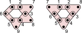
Figure 1. Collections $\mathcal{C}_{1}$ and $\mathcal{C}_{2}$ of subsets

Example 4.2.

Let $S_{9}\stackrel{{\scriptstyle\text{\tiny def}}}{{=}}\{1,2,\ldots,9\}$. Consider two collections of subsets of $S_{9}$ shown on fig.1. In the first collection there are no $A_{1},A_{2},A_{3}\in\mathcal{C}_{1}$ such that $A_{1}\cup A_{2}\cup A_{3}=S_{9}$. On the other hand there exist $A_{1},A_{2},A_{3}\in\mathcal{C}_{2}$ such that $A_{1}\cup A_{2}\cup A_{3}=S_{9}$.

Now consider simplicial complexes $L_{1}$ and $L_{2}$ with $N(L_{i})=\{I\subset S_{9}\mid S_{9}\setminus I\in\mathcal{C}_{i}\}$ for $i=1,2$. Then condition (3) of Statement 4.1 does not hold for $L_{1}$, but holds for $L_{2}$. Statement 4.1 implies $s(L_{1})=1$ and $s(L_{2})\geqslant 2$ (and the same for $s_{\mathbb{R}}$).

Remark 4.3.

One can consider collections $\mathcal{C}_{1}$ and $\mathcal{C}_{2}$ as simplicial complexes. Then the complexes $L_{i}$ are Alexander duals of $\mathcal{C}_{i}$ by the definition of combinatorial Alexander duality (see e.g. [6, Ex.2.26]).

4.3. Bigraded Betti numbers and Taylor resolution

First, we review the basics of commutative algebra needed to define bigraded Betti numbers.

Let $\Bbbk$ be a ground field and $\Bbbk[m]=\Bbbk[v_{1},\ldots,v_{m}]$ — the polynomial algebra graded by $\deg v_{i}=2$. Also define the multigrading by $\operatorname{mdeg}(v_{1}^{n_{1}}\cdot\ldots\cdot v_{m}^{n_{m}})=(2n_{1},\ldots,2n_{m})\in\mathbb{Z}^{m}$. Denote by $\Bbbk[m]^{+}$ the maximal graded ideal of $\Bbbk[m]$ — i.e. the ideal generated by monomials of positive degrees.

The Stanley–Reisner algebra (otherwise called the face ring) of a simplicial complex $K$ on $m$ vertices is the quotient algebra $\Bbbk[K]=\Bbbk[m]/I_{SR}(K)$, where $I_{SR}(K)$ is the square-free ideal generated by monomials, corresponding to non-simplices of $K$:

$$I_{SR}(K)=(v_{i_{1}}\cdot\ldots\cdot v_{i_{k}}\mid\{i_{1},\ldots,i_{k}\}\notin K);$$

Both $\Bbbk$ and $\Bbbk[K]$ carry the structure of (multi)graded $\Bbbk[m]$-modules via quotient epimorphisms $\Bbbk[m]\to\Bbbk[m]/\Bbbk[m]^{+}\cong\Bbbk$ and $\Bbbk[m]\to\Bbbk[K]$. Then $\operatorname{Tor}^{*,*}_{\Bbbk[m]}(\Bbbk[K],\Bbbk)$ is a $\operatorname{Tor}$-functor of (multi)graded modules $\Bbbk[K]$ and $\Bbbk$. Recall its standard construction in homological algebra.

Construction 4.4.

To describe $\operatorname{Tor}^{*,*}_{\Bbbk[m]}(\Bbbk[K],\Bbbk)$ do the following:

1. Take any free resolution of the module $\Bbbk[K]$ by (multi)graded $\Bbbk[m]$-modules:

   $$\ldots\xrightarrow{d}R^{-\ell}\xrightarrow{d}R^{-\ell+1}\xrightarrow{d}\ldots\to R^{-1}\to R^{0}\xrightarrow{d}\Bbbk[K]\qquad(\mathcal{R})$$

2. apply the functor $\otimes_{\Bbbk[m]}\Bbbk$;

3. take cohomology of the resulting complex:

   $$\operatorname{Tor}^{*,*}_{\Bbbk[m]}(\Bbbk[K],\Bbbk)\stackrel{{\scriptstyle\text{\tiny def}}}{{\cong}}H^{*}(\mathcal{R}^{*}\otimes_{\Bbbk[m]}\Bbbk;d\otimes_{\Bbbk[m]}\Bbbk)$$

The resulting vector space inherits inner (multi)grading from $\mathcal{R}$. It also obtains an additional grading $-\ell$. It is well known that $\operatorname{Tor}^{*,*}_{\Bbbk[m]}(\Bbbk[K],\Bbbk)\cong\bigoplus_{(\ell,\bar{j})\in\mathbb{Z}^{m+1}}\operatorname{Tor}^{-\ell,2\bar{j}}_{\Bbbk[m]}(\Bbbk[K],\Bbbk)$ does not depend on the choice of a free (multi)graded resolution $\mathcal{R}$. Define bigraded Betti numbers of $K$ as

$$\beta^{-\ell,2j}(K)\stackrel{{\scriptstyle\text{\tiny def}}}{{=}}\dim_{\Bbbk}\operatorname{Tor}_{\Bbbk[m]}^{-\ell,2j}(\Bbbk[K],\Bbbk).$$

Definition 4.5 (Minimal resolution).

A resolution $\mathcal{R}$ is called minimal if $\operatorname{im}(d)\subset\Bbbk[m]^{+}\cdot\mathcal{R}$, or, equivalently, $d\otimes_{\Bbbk[m]}\Bbbk=0$.

For a minimal resolution $\mathcal{R}$ step (3) in Construction 4.4 is skipped. Therefore:

$$\beta^{-\ell,2j}(K)=\mbox{number of generators of the module }R^{-\ell}\mbox{ in degree }2j.$$

Several explicit constructions of free resolutions of $\Bbbk[K]$ are known. In our considerations we use one of the most important and basic constructions — the Taylor resolution. In general, Taylor resolution is defined for any monomial ideal (see [25] or [24]). Here we concentrate only on the case of Stanley–Reisner rings, i.e. the case of square-free monomial ideals. The work [27] is also concerned with this particular case.

In the sequel the following convention is used. Any subset $B\subseteq[m]$ determines the vector $\delta_{B}\in\mathbb{Z}^{m}$ with $i$-th coordinate equal to $1$ if $i\in B$ and $0$ otherwise. We simply write $B\in\mathbb{Z}^{m}$ meaning $\delta_{B}\in\mathbb{Z}^{m}$. For a set $B$ we denote the monomial $\overline{v}^{\delta_{B}}=v_{1}^{\delta_{B}^{1}}\ldots v_{m}^{\delta_{B}^{m}}\in\Bbbk[m]$ simply by $v^{B}$.

Construction 4.6 (Taylor resolution).

Consider the set $N(K)$ of minimal non-simplices. Fix a linear order on $N(K)$. For each $J\in N(K)$ associate a formal variable $w_{J}$ and construct the free $\Bbbk[m]$-module

$$R_{T}^{-\ell}\stackrel{{\scriptstyle\text{\tiny def}}}{{=}}\Lambda^{\ell}[\{w_{J}\}]\otimes\Bbbk[m]$$

Here $\Lambda^{\ell}[\{w_{J}\}]$ is the vector space over $\Bbbk$, generated by formal expressions $W_{\sigma}=w_{J_{1}}\wedge\ldots\wedge w_{J_{\ell}}$ for all subsets $\sigma=\{J_{1},\ldots,J_{\ell}\}\subseteq N(K)$, $J_{1}<\ldots<J_{\ell}$.

Define the multigrading

(4.1) $$\operatorname{mdeg}(w_{J_{1}}\wedge\ldots\wedge w_{J_{\ell}})\stackrel{{\scriptstyle\text{\tiny def}}}{{=}}\left(-\ell,2\bigcup_{i=1}^{\ell}J_{i}\right)\in\mathbb{Z}\times\mathbb{Z}^{m},$$

and the double grading

$$\operatorname{bideg}(w_{J_{1}}\wedge\ldots\wedge w_{J_{\ell}})\stackrel{{\scriptstyle\text{\tiny def}}}{{=}}\left(-\ell,2\left|\bigcup_{i=1}^{\ell}J_{i}\right|\right)\in\mathbb{Z}^{2}.$$

The first component is called a homological grading.

Define the differential of $\Bbbk[m]$-modules $d_{T}\colon R_{T}^{-\ell}\to R_{T}^{-\ell+1}$ on the generators $W_{\sigma}=w_{J_{1}}\wedge\ldots\wedge w_{J_{\ell}}$ by

(4.2) $$d_{T}(w_{J_{1}}\wedge\ldots\wedge w_{J_{\ell}})\stackrel{{\scriptstyle\text{\tiny def}}}{{=}}\sum\limits_{i=1}^{\ell}(-1)^{i+1}v^{X_{\sigma,J_{i}}}\cdot w_{J_{1}}\wedge\ldots\widehat{w_{J_{i}}}\ldots\wedge w_{J_{\ell}},$$

where $v^{X_{\sigma,J_{i}}}\in\Bbbk[m]$ is the monomial corresponding to the set

$$X_{\sigma,J_{i}}\stackrel{{\scriptstyle\text{\tiny def}}}{{=}}J_{i}\setminus\left(J_{1}\cup\ldots\widehat{J_{i}}\ldots\cup J_{\ell}\right)\subset[m].$$

Define the multiplication on the $\Bbbk[m]$-module $\mathcal{R}_{T}=\bigoplus_{\ell}R_{T}^{-\ell}$ by describing the products of generators. Let $\sigma=\{J_{1}<\ldots<J_{\ell}\},\tau=\{I_{1}<\ldots<I_{k}\}\subseteq N(K)$.

(4.3) $$W_{\sigma}\cdot W_{\tau}\stackrel{{\scriptstyle\text{\tiny def}}}{{=}}\begin{cases}0,\mbox{ if }\sigma\cap\tau\neq\varnothing;\\ \operatorname{sgn}(\sigma,\tau)v^{Y_{\sigma,\tau}}W_{\sigma\sqcup\tau},\mbox{ otherwise.}\end{cases}$$

Here $v^{Y_{\sigma,\tau}}\in\Bbbk[m]$ is the monomial corresponding to the set of indices $Y_{\sigma,\tau}=(\bigcup_{\sigma}J_{i})\cap(\bigcup_{\tau}I_{i})$. The sign $\operatorname{sgn}(\sigma,\tau)$ is the sign of the permutation needed to sort the unordered set $(J_{1},\ldots,J_{\ell},I_{1},\ldots,I_{k})$.

Proposition 4.7 ([25],[24]).

1. The vector space $\mathcal{R}_{T}=\bigoplus_{\ell}R_{T}^{-\ell}$ is a differential $\mathbb{Z}^{m+1}$-graded algebra over the ring $\Bbbk[m]$ w.r.t. to the multigrading, the differential, and the multiplication described above. This algebra is skew-commutative with respect to homological grading.

2. $H^{-\ell}(\mathcal{R}_{T},d)=0$ if $\ell>0$. $H^{0}(\mathcal{R}_{T},d)\cong\Bbbk[K]$ as $\Bbbk[m]$-algebras.

Therefore, $\mathcal{R}_{T}$ is a free multiplicative resolution of a Stanley–Reisner algebra $\Bbbk[K]$.

Example 4.8.

Let $o_{m}$ be a simplicial complex on a set $[m]$ in which all vertices are ghost. We have $\Bbbk[o_{m}]\cong\Bbbk$ and $N(o_{m})=[m]$. The Taylor resolution in this case is given by $R_{T}^{-\ell}=\Lambda^{\ell}[u_{1},\ldots,u_{m}]\otimes\Bbbk[m]$, where formal variables $u_{i}$ correspond to elements of $N(o_{m})=[m]$ and $\operatorname{bideg}u_{i}=(-1,2)$. By looking at general definitions of differential and product we see that $\mathcal{R}_{T}$ is isomorphic to $\Lambda[u_{1},\ldots,u_{m}]\otimes\Bbbk[m]$ with the standard Grassmann product, and the differential given by $du_{i}=v_{i}$. In this example we get the multiplicative resolution $\Lambda[u_{1},\ldots,u_{m}]\otimes\Bbbk[m]$ of the $\Bbbk[m]$-module $\Bbbk$. This resolution is widely known as Koszul resolution.

Example 4.9.

Let $K$ be the boundary of a square. Its maximal simplices are $\{1,2\}$, $\{2,3\}$, $\{3,4\}$, $\{1,4\}$. In this case $N(K)=\{\{1,3\},\{2,4\}\}$. The Taylor resolution has the form

with the multigrading

$$\operatorname{mdeg}(w_{\{1,3\}}) =(-1;(2,0,2,0)),$$

$$\operatorname{mdeg}(w_{\{2,4\}}) =(-1;(0,2,0,2)),$$

$$\operatorname{mdeg}(W_{\{\{1,3\},\{2,4\}\}}) =(-2;(2,2,2,2)),$$

the differentials

$$d_{1}(w_{\{1,3\}}) =v_{1}v_{3}\cdot 1,$$

$$d_{1}(w_{\{2,4\}}) =v_{2}v_{4}\cdot 1,$$

$$d_{2}(W_{\{\{1,3\},\{2,4\}\}}) =v_{1}v_{3}\cdot w_{\{2,4\}}-v_{2}v_{4}\cdot w_{\{1,3\}},$$

and the product $w_{\{1,3\}}\times w_{\{2,4\}}=W_{\{\{1,3\},\{2,4\}\}}=-w_{\{2,4\}}\times w_{\{1,3\}}$. Clearly, $\operatorname{im}(d_{2})=\ker(d_{1})$ and $\operatorname{im}(d_{1})=I_{SR}(K)$.

Example 4.10.

Let $\Delta_{M}$ denote a simplex on a set $M\neq\varnothing$. Consider $K=\partial\leavevmode\nobreak\ \Delta_{M_{1}}\leavevmode\nobreak\ \ast\leavevmode\nobreak\ \ldots\leavevmode\nobreak\ \ast\leavevmode\nobreak\ \partial\leavevmode\nobreak\ \Delta_{M_{k}}$ — a simplicial sphere on a set $M_{1}\sqcup\ldots\sqcup M_{n}$. Then $N(K)=\{M_{1},\ldots,M_{n}\}$. The Taylor resolution of $K$ is a differential algebra

$$\Lambda^{*}[w_{1},\ldots,w_{n}]\otimes\Bbbk[M_{1}\sqcup\ldots\sqcup M_{n}]$$

with the standard Grassmann product, $\operatorname{bideg}(w_{i})=(-1,2|M_{i}|)$, and differential:

$$d_{T}(w_{i_{1}}\wedge\ldots\wedge w_{i_{\ell}})=\sum\limits_{k=1}^{\ell}(-1)^{k+1}v^{M_{i_{k}}}w_{i_{1}}\wedge\ldots\widehat{w_{i_{k}}}\ldots\wedge w_{i_{\ell}}.$$

The Taylor resolution is minimal, therefore $\operatorname{Tor}^{*,*}_{\Bbbk[M_{1}\sqcup\ldots\sqcup M_{n}]}(\Bbbk[K];\Bbbk)\cong\Lambda^{*}[w_{1},\ldots,w_{n}]$. Both previous examples are the particular cases of this one.

4.4. Multiplication in $\operatorname{Tor}$

Construction 4.11.

There is a standard way to understand the structure of $\operatorname{Tor}^{*,*}_{\Bbbk[m]}(\Bbbk[K];\Bbbk)$ using Koszul resolution. At first, note that $\operatorname{Tor}^{*,*}_{\Bbbk[m]}(\Bbbk[K];\Bbbk)\cong\operatorname{Tor}^{*,*}_{\Bbbk[m]}(\Bbbk;\Bbbk[K])$. By construction,

$$\operatorname{Tor}^{*,*}_{\Bbbk[m]}(\Bbbk;\Bbbk[K])\cong H^{*}(\mathcal{R}\otimes_{\Bbbk[m]}\Bbbk[K];d\otimes_{\Bbbk[m]}\Bbbk[K]),$$

where $(\mathcal{R}^{*},d)$ is any graded free resolution of $\Bbbk$ as a $\Bbbk[m]$-module. Take for example Koszul resolution $\mathcal{R}^{-\ell}\cong\Lambda[u_{1},\ldots,u_{m}]\otimes\Bbbk[m]$ with grading and differential as described in Example 4.8. Then

(4.4) $$\operatorname{Tor}^{*,*}_{\Bbbk[m]}(\Bbbk;\Bbbk[K])\cong H^{*}(\Lambda[u_{1},\ldots,u_{m}]\otimes\Bbbk[K];d\otimes_{\Bbbk[m]}\Bbbk[K]).$$

The differential complex $\Lambda[u_{1},\ldots,u_{m}]\otimes\Bbbk[K]$ has the structure of a differential graded algebra. Thus $\operatorname{Tor}^{*,*}_{\Bbbk[m]}(\Bbbk;\Bbbk[K])$ has the structure of an algebra as well. The word ‘‘$\operatorname{Tor}$-algebra’’ usually refers to this definition of a multiplication.

Statement 4.12 ([5, 15]).

The cohomology ring $H^{*}(\mathcal{Z}_{K};\Bbbk)$ is isomorphic as a graded algebra to the $\operatorname{Tor}$-algebra $\operatorname{Tor}^{*,*}_{\Bbbk[m]}(\Bbbk[K];\Bbbk)$ with the total grading $(-i,2j)\rightsquigarrow 2j-i$.

Remark 4.13.

According to Construction 4.4,

(4.5) $$\operatorname{Tor}^{*,*}_{\Bbbk[m]}(\Bbbk[K];\Bbbk)\cong H^{*}(\mathcal{R}_{T}\otimes_{\Bbbk[m]}\Bbbk;d_{T}\otimes_{\Bbbk[m]}\Bbbk),$$

where $(\mathcal{R}_{T},d_{T})$ is the Taylor resolution of $\Bbbk[K]$. The differential complex $\mathcal{R}_{T}\otimes_{\Bbbk[m]}\Bbbk$ obtains the multiplication from the multiplication in the Taylor resolution. This, in turn, induces the multiplication on $H^{*}(\mathcal{R}_{T}\otimes_{\Bbbk[m]}\Bbbk;d_{T}\otimes_{\Bbbk[m]}\Bbbk)$. A priori it is not clear, whether this multiplication on $\operatorname{Tor}^{*,*}_{\Bbbk[m]}(\Bbbk[K];\Bbbk)$ is the same as given by Construction 4.11 or not. Fortunately, this multiplicative structures are indeed the same (see e.g. [1, Constr. 2.3.2]). So far the cohomological product in $H^{*}(\mathcal{Z}_{K};\Bbbk)$ in some cases can be described in terms of the Taylor resolution [27].

4.5. Taylor resolutions and minimality

When the Taylor resolution is minimal, the benefits of both notions — Taylor resolution and minimality — can be used.

Lemma 4.14.

Let $K$ be a simplicial complex on $[m]$ and $N(K)$ — the set of minimal non-simplices. The following conditions are equivalent:

1. The Taylor resolution $(\mathcal{R}_{T},d_{T})$ of $\Bbbk[K]$ is minimal.

2. Any minimal simplex $J\in N(K)$ is not a subset in the union of others:

   (4.6) $$J\nsubseteq\bigcup_{I\in N(K),I\neq J}I.$$

Proof.

By definition, $\mathcal{R}_{T}$ is minimal if $d_{T}(R_{T}^{-\ell})\subseteq\Bbbk[m]^{+}\cdot R_{T}^{-\ell+1}$ for each $\ell\geqslant 0$. From (4.2) follows that $d_{T}(R_{T}^{-\ell})\subseteq\Bbbk[m]^{+}\cdot R_{T}^{-\ell+1}$ if and only if $v^{X_{\sigma,J}}\in\Bbbk[m]^{+}$ for each $\sigma\subseteq N(K)$ and $J\in\sigma$. This is equivalent to $X_{\sigma,J}\neq\varnothing$. By definition, $X_{\sigma,J}=J\setminus\left(\bigcup_{I\in\sigma,I\neq J}I\right)$. If the Taylor resolution is minimal, then, in particular, $X_{N(K),J}\neq\varnothing$, which is precisely the condition (4.6) of the lemma. On the other hand, $X_{N(K),J}\neq\varnothing$ implies $X_{\sigma,J}\neq\varnothing$ for any $\sigma\subseteq N(K)$. ∎

Lemma 4.15.

If the Taylor resolution of $\Bbbk[K]$ is minimal, then $\operatorname{Tor}^{*,*}_{\Bbbk[m]}(\Bbbk[K],\Bbbk)$ has the following description:

• It is generated as a vector space over $\Bbbk$ by $W_{\sigma}$ for $\sigma\subseteq N(K)$;

• The multidegree is given by (4.1);

• The multiplication is given by

  (4.7) $$W_{\sigma}\cdot W_{\tau}=\begin{cases}\operatorname{sgn}(\sigma,\tau)W_{\sigma\sqcup\tau},\mbox{ if }\sigma\cap\tau=\varnothing\mbox{ and }(\bigcup_{J\in\sigma}J)\cap(\bigcup_{I\in\tau}I)=\varnothing\\ 0,\mbox{ otherwise.}\end{cases}$$

The proof follows easily from the construction of Taylor resolution and the definition of minimality.

For complexes with the minimal Taylor resolution bigraded Betti numbers are expressed in combinatorial terms.

(4.8) $$\beta^{-\ell,2j}(K)=\#\left\{\sigma\subseteq N(K)\middle||\sigma|=\ell,\left|\bigcup_{J\in\sigma}J\right|=j\right\}$$

4.6. Proof of Theorem 2

At last, we have all necessary ingredients to prove Theorem 2. As a starting point take complexes $L_{1}$ and $L_{2}$ defined in Example 4.2. Our plan is the following:

1. To upgrade $L_{1}$ and $L_{2}$ to the new complexes $K_{1}$ and $K_{2}$ satisfying condition (4.6) (Taylor resolution is minimal);

2. To prove that $\beta^{-\ell,2j}(K_{1})=\beta^{-\ell,2j}(K_{2})$ using formula (4.8);

3. To prove that $s(K_{1})=1$ and $s(K_{2})\geqslant 2$.

4. Final technical remarks: $\dim(K_{1})=\dim(K_{2})$, $\gamma(K_{1})=\gamma(K_{2})$, and algebra isomorphism $\operatorname{Tor}_{\Bbbk[m]}(\Bbbk[K_{1}],\Bbbk)\cong\operatorname{Tor}_{\Bbbk[m]}(\Bbbk[K_{2}],\Bbbk)$.

Step 1. Let $L$ be any complex on a set $[m]$ with the set of minimal non-simplices $N(L)$. For each $J\in N(L)$ consider a symbol $a_{J}$. Define the complex ${\widetilde{L}}$ on the set $V=[m]\sqcup\{a_{J}\mid J\in N(K)\}$ with the set of minimal non-simplices given by

(4.9) $${\widetilde{J}}\in N({\widetilde{L}})\Leftrightarrow{\widetilde{J}}=J\sqcup\{a_{J}\}\subset V\mbox{ for }J\in N(K)$$

The Taylor resolution of the complex ${\widetilde{L}}$ is minimal. Indeed, any ${\widetilde{J}}\in N({\widetilde{L}})$ contains the vertex $a_{J}$ which does not belong to other minimal non-simplices. Therefore, condition (4.6) holds for ${\widetilde{L}}$.

Now we apply this construction to $L_{1}$ and $L_{2}$. Recall that $N(L_{i})=\{I\subset S_{9}\mid S_{9}\setminus I\in\mathcal{C}_{i}\}$ for $i=1,2$ and collections of subsets $\mathcal{C}_{1},\mathcal{C}_{2}$ shown on fig.1. Set $K_{i}={\widetilde{L_{i}}}$ for $i=1,2$. Both $K_{1}$ and $K_{2}$ have $9+6=15$ vertices.

Step 2. Apply (4.8) to $K_{i}$:

(4.10) $$\beta^{-\ell,2j}(K_{i})=\#\left\{\sigma\subseteq N(K_{i})\middle||\sigma|=\ell,\left|\bigcup_{{\widetilde{J}}\in\sigma}{\widetilde{J}}\right|=j\right\}=\\ \#\left\{\sigma\subseteq N(L_{i})\middle||\sigma|=\ell,\left|\bigcup_{J\in\sigma}{\widetilde{J}}\right|=j\right\}.$$

The last equality is the consequence of bijective correspondence between $N(L_{i})$ and $N(K_{i})$, sending $J\in N(L_{i})$ to ${\widetilde{J}}\in N(K_{i})$. We have

$$\bigcup_{J\in\sigma}{\widetilde{J}}=\bigcup_{J\in\sigma}(J\sqcup\{a_{J}\})=\left(\bigcup_{J\in\sigma}J\right)\sqcup\{a_{J}\mid J\in\sigma\},$$

therefore

$$\left|\bigcup_{J\in\sigma}{\widetilde{J}}\right|=\left|\bigcup_{J\in\sigma}J\right|+|\sigma|.$$

Returning to (4.10),

(4.11) $$\beta^{-\ell,2j}(K_{i})=\#\left\{\sigma\subseteq N(L_{i})\middle||\sigma|=\ell,\left|\bigcup_{J\in\sigma}{\widetilde{J}}\right|=j\right\}=\\ =\#\left\{\sigma\subseteq N(L_{i})\middle||\sigma|=\ell,\left|\bigcup_{J\in\sigma}J\right|=j-\ell\right\}=\\ =\#\left\{\sigma\subseteq\mathcal{C}_{i}\middle||\sigma|=\ell,\left|\bigcap_{A\in\sigma}A\right|=9-(j-\ell)\right\}.$$

The last equality follows from the definition of $L_{i}$, since $N(L_{i})$ consists of complements to subsets of the collection $\mathcal{C}_{i}$. By analyzing fig.1 we see that for each $\ell$ and $j$

$$\#\left\{\sigma\subseteq\mathcal{C}_{1}\middle||\sigma|=\ell,\left|\bigcap_{A\in\sigma}A\right|=9-(j-\ell)\right\}=\#\left\{\sigma\subseteq\mathcal{C}_{2}\middle||\sigma|=\ell,\left|\bigcap_{A\in\sigma}A\right|=9-(j-\ell)\right\}.$$

Indeed, in both $\mathcal{C}_{1}$ and $\mathcal{C}_{2}$ there are $3$ subsets of cardinality $2$, $3$ subsets of cardinality $3$, $6$ pairwise intersections of cardinality $1$, and all other intersections are empty. Therefore, $\beta^{-\ell,2j}(K_{1})=\beta^{-\ell,2j}(K_{2})$. The nonzero bigraded Betti numbers calculated by the described method are presented in fig.2 (empty cells are filled with zeroes).

Figure 2. Bigraded Betti numbers of $K_{1}$ and $K_{2}$

Step 3. We use the following simple observation. Condition (3) of Statement 4.1 holds for the complex $L$ whenever it holds for ${\widetilde{L}}$. Indeed, ${\widetilde{J_{1}}}\cap{\widetilde{J_{2}}}\cap{\widetilde{J_{3}}}=(J_{1}\sqcup\{a_{J_{1}}\})\cap(J_{2}\sqcup\{a_{J_{2}}\})\cap(J_{3}\sqcup\{a_{J_{1}}\})=J_{1}\cap J_{2}\cap J_{3}$. As observed in Example 4.2 condition (3) of Statement 4.1 holds for $L_{2}$ and does not hold for $L_{1}$. Therefore it also holds for $K_{2}={\widetilde{L_{2}}}$ and does not hold for $K_{1}={\widetilde{L_{1}}}$. Thus $s(K_{1})\neq s(K_{2})$ and $s_{\mathbb{R}}(K_{1})\neq s_{\mathbb{R}}(K_{2})$.

Step 4. Final remarks.

Remark 4.16.

Let us prove that $\dim K_{1}=\dim K_{2}=12$. Consider the complement to the set $\{1,4\}$ in the set of vertices of $K_{1}$ (see fig. 1):

$$S=\{1,2,\ldots,9,a_{1},\ldots,a_{6}\}\setminus\{1,4\}.$$

Suppose that $S\notin K_{1}$. Then there exists ${\widetilde{J}}\in N(K_{1})$ such that ${\widetilde{J}}\subseteq S$. Therefore, $\{1,4\}=S_{9}\setminus S\subseteq S_{9}\setminus{\widetilde{J}}$. By construction, $S_{9}\setminus{\widetilde{J}}\in\mathcal{C}_{1}$. But $\{1,4\}$ is not contained in any $A\in\mathcal{C}_{1}$ — the contradiction. Thus $S\in K_{1}$ and $\dim K_{1}\geqslant|S|-1=12$. Similar reasoning shows that there is no simplex in $K_{1}$ of cardinality $14$ (because any singleton lies in some $A\in\mathcal{C}_{1}$). Therefore $\dim K_{1}$ is exactly $12$. Same for $K_{2}$.

Remark 4.17.

In both complexes $K_{1}$ and $K_{2}$ there are no minimal non-simplices of cardinality $1$ and $2$. Therefore all pairs of vertices in $K_{1}$ and $K_{2}$ are connected by edges, so $1$-skeletons $K_{1}^{(1)}$, $K_{2}^{(1)}$ are complete graphs on $15$ vertices. Thus chromatic numbers coincide $\gamma(K_{1})=\gamma(K_{2})=15$.

Remark 4.18.

$\operatorname{Tor}$-algebras of $K_{1}$ and $K_{2}$ are isomorphic as algebras. Actually, the products in $\operatorname{Tor}_{\Bbbk[15]}(\Bbbk[K_{1}],\Bbbk)$ and $\operatorname{Tor}_{\Bbbk[15]}(\Bbbk[K_{2}],\Bbbk)$ are trivial by dimensional reasons (see fig. 2): products of nonzero elements always hit zero cells. The triviality of multiplication can be deduced also from Lemma 4.15 but this approach requires a complicated combinatorial reasoning.

These remarks conclude the proof of Theorem 2.

4.7. Other invariants coming from $\mathcal{Z}_{K}$

Remark 4.19.

Question 1.4 is answered in the negative if $A(\cdot)$ is a collection of bigraded Betti numbers. We may ask the same question for $A(\cdot)$ — the collection of all multigraded Betti numbers $\beta^{-i,2\overline{j}}(K)\stackrel{{\scriptstyle\text{\tiny def}}}{{=}}\dim\operatorname{Tor}_{\Bbbk[m]}^{-i,2\overline{j}}(\Bbbk[K],\Bbbk)$.

Eventually, this question does not make sense. Multigraded Betti numbers are too strong invariants: $\beta^{-1,2\overline{j}}(K)=\beta^{-1,2\overline{j}}(L)$ implies $K=L$. Indeed, for a subset $A\subseteq[m]$ the condition $\beta^{-1,2A}(K)\neq 0$ is equivalent to $A\in N(K)$ by the construction of the Taylor resolution (also by Hochster’s formula [7, Th.3.2.9]). Therefore multigraded Betti numbers encode all minimal non-simplices and determine the complex $K$ uniquely.

Remark 4.20.

Question 1.4 may be formulated for an equivariant cohomology ring of $\mathcal{Z}_{K}$. This task is not interesting as well. Indeed, $H^{*}_{T^{m}}(\mathcal{Z}_{K};\Bbbk)\cong\Bbbk[K]$ (see [9] or [5]). It is known, that the Stanley–Reisner algebra $\Bbbk[K]$ determines the combinatorics of $K$ uniquely [4]. Therefore multiplicative isomorphism $H^{*}_{T^{m}}(\mathcal{Z}_{K_{1}};\Bbbk)\cong H^{*}_{T^{m}}(\mathcal{Z}_{K_{2}};\Bbbk)$ implies $K_{1}\cong K_{2}$ and, in particular, $s(K_{1})=s(K_{2})$.

5. Conclusion and open questions

Constructions of Buchstaber invariants and bigraded Betti numbers are defined for any simplicial complex. Nevertheless, in toric topology the most important are simplicial complexes arising from polytopes.

Let $P$ be a simple polytope with $m$ vertices. The polar dual polytope $P^{*}$ is simplicial. The complex $K_{P}=\partial P^{*}$ is a simplicial sphere with $m$ vertices. It is known [5, 6] that $\mathcal{Z}_{K_{P}}$ is a smooth compact manifold and the action of $T^{m}$ on $\mathcal{Z}_{K_{P}}$ is smooth. The algebraic version of this fact is Avramov–Golod theorem [7, Th.3.4.4]. It states the following. The $\operatorname{Tor}$-algebra $\operatorname{Tor}^{*,*}_{\Bbbk[m]}(\Bbbk[K];\Bbbk)$ is a (multigraded) Poincare duality algebra if and only if the complex $K$ is Gorenstein*. Any simplicial sphere $K$ is Gorenstein* [26, Th.5.1]. In particular, for any simple polytope $P$ the complex $K_{P}$ is Gorenstein*, thus $\operatorname{Tor}^{*,*}_{\Bbbk[m]}(\Bbbk[K_{P}];\Bbbk)$ is a Poincare duality algebra. This is not surprising since $\operatorname{Tor}^{*,*}_{\Bbbk[m]}(\Bbbk[K_{P}];\Bbbk)\cong H^{*}(\mathcal{Z}_{K_{P}};\Bbbk)$ and $\mathcal{Z}_{K_{P}}$ is a manifold.

The problems solved in this paper can be posed for particular classes of simplicial complexes, for example boundaries of simplicial polytopes or simplicial spheres.

Problem 1.

Does $s(K_{P})=s_{\mathbb{R}}(K_{P})$ for any simple polytope $P$?

The complex $U={{}_{\mathbb{R}}U}_{4}$ constructed in the proof of Theorem 1 is not a boundary of a polytope; it is not a simplicial sphere as well. Nevertheless, $U$ is Cohen–Macaulay as proved in [9, Th.2.2].

Another problem can also be formulated for the class of polytopes.

Problem 2.

Does $\beta^{-i,2j}(K_{P})=\beta^{-i,2j}(K_{Q})$ imply $s(K_{P})=s(K_{Q})$ or $s_{\mathbb{R}}(K_{P})=s_{\mathbb{R}}(K_{Q})$ for simple polytopes $P$ and $Q$? If no, does an isomorphism of algebras $\operatorname{Tor}^{*,*}_{\Bbbk[m]}(\Bbbk[K_{P}];\Bbbk)\cong\operatorname{Tor}^{*,*}_{\Bbbk[m]}(\Bbbk[K_{Q}];\Bbbk)$ imply $s(K_{P})=s(K_{Q})$ or $s_{\mathbb{R}}(K_{P})=s_{\mathbb{R}}(K_{Q})$?

The complexes $K_{1}$ and $K_{2}$ constructed in Section 4 are not simplicial spheres as well. One can deduce this from the table of bigraded Betti numbers (fig. 2): if the complexes were spheres the distribution of bigraded Betti numbers would be symmetric according to (bigraded) Poincare duality.

It is tempting to modify the construction of $K_{1}$ and $K_{2}$ of Section 4 to obtain polytopal spheres in the output. Unfortunately, this attempt fails due to the following observation.

Proposition 5.1.

Let $K$ be a simplicial sphere. The Taylor resolution of $\Bbbk[K]$ is minimal if and only if $K$ is a join of boundaries of simplices.

Remark 5.2.

For such $K$ it is easily shown that $s(K)=s_{\mathbb{R}}(K)=m\leavevmode\nobreak\ -\leavevmode\nobreak\ \dim\leavevmode\nobreak\ K\leavevmode\nobreak\ -\leavevmode\nobreak\ 1$. Thus a counterexample to Problem 2 can not be constructed using minimal Taylor resolutions.

Proof of the proposition.

The ‘‘if’’ part is Example 4.10. Let us prove the ‘‘only if’’ part. Let $[m]$ be the vertex set of $K$. Any vertex $i\in[m]$ is contained in at least one minimal non-simplex. Otherwise, $K$ is a cone with the apex $i$, so $K$ is not a sphere. Since the Taylor resolution is minimal, we may apply Lemma 4.15. Complex $K$ is a sphere, thus $\Bbbk[K]$ is Gorenstein* and $\operatorname{Tor}^{*,*}_{\Bbbk[m]}(\Bbbk[K];\Bbbk)$ is a multigraded Poincare duality algebra. There should be a graded component of $\operatorname{Tor}^{*,*}_{\Bbbk[m]}(\Bbbk[K];\Bbbk)$ of maximal total degree which plays the role of the ‘‘fundamental cycle’’. Obviously, this component is generated by $W_{N(K)}$ in the notation of Lemma 4.15. This component has multidegree $(-|N(K)|,(2,2,\ldots,2))$. Non-degenerate pairing in Poincare duality algebra $\operatorname{Tor}^{*,*}_{\Bbbk[m]}(\Bbbk[K];\Bbbk)$ yields that for each $\sigma\subseteq N(K)$ exists $\tau\subseteq N(K)$ such that $W_{\sigma}\cdot W_{\tau}=\alpha W_{N(K)}$ with $\alpha\neq 0$. Taking multigrading into account and applying Lemma 4.15 we get the following condition: for each $\sigma\subseteq N(K)$ the vertex subsets $\bigcup_{J\in\sigma}J$ and $\bigcup_{J\in N(K)\setminus\sigma}J$ are disjoint. In particular, any single non-simplex $J\in N(K)$ is disjoint from the union of others. Therefore, $N(K)=\{J_{1},\ldots,J_{k}\}$ and $[m]=J_{1}\sqcup\ldots\sqcup J_{k}$. Thus $K=(\partial\Delta_{J_{1}})\ast\ldots\ast(\partial\Delta_{J_{k}})$ which was to be proved. ∎

References

- [1] Luchezar L.Avramov, Infinite free resolutions, Six lectures on commutative algebra (Bellaterra, 1996), Progr. Math. 166, Birkhauser, Basel, 1998; pp. 1–118.
- [2] A. Ayzenberg, The problem of Buchstaber number and its combinatorial aspects, arXiv:1003.0637.
- [3] A. Ayzenberg, Relation between the Buchstaber invariant and generalized chromatic numbers, Dal’nevost.Mat. Zh., 11:2 (2011), 113–139.
- [4] W. Bruns, J. Gubeladze, Combinatorial invariance of Stanley-Reisner rings, Georgian Mathematical Journal, V.3, N.4, (1996), pp. 315–318.
- [5] V. M. Bukhshtaber and T. E. Panov, Torus actions, combinatorial topology, and homological algebra, Russian Mathematical Surveys(2000),55(5):825
- [6] V. M. Buchstaber and T. E. Panov, Torus Actions and Their Applications in Topology and Combinatorics, Univ. Lecture Ser. 24 (2002).
- [7] Victor Buchstaber, Taras Panov, Toric Topology, preprint arXiv:1210.2368
- [8] On the quantum chromatic number of a graph, Peter J. Cameron, Michael W. Newman, Ashley Montanaro, Simone Severini, and Andreas Winter, Electronic Journal of Combinatorics 14(1), 2007
- [9] M. Davis, T. Januszkiewicz, Convex polytopes, Coxeter orbifolds and torus actions, Duke Math. J., 62:2 (1991), 417–451.
- [10] Nickolai Erokhovets, Maximal torus actions on moment-angle manifolds, doctoral thesis, Moscow State University, 2011 (in russian).
- [11] Nikolai Yu. Erokhovets, Buchstaber invariant of simple polytopes, Russian Math. Surveys, 63:5 (2008), 962–964.
- [12] Nickolai Erokhovets, Buchstaber Invariant of Simple Polytopes, preprint arXiv:0908.3407
- [13] Nickolai Erokhovets, Criterion for the Buchstaber invariant of simplicial complexes to be equal to two, preprint arXiv:1212.3970
- [14] Nickolai Erokhovets, The theory of Buchstaber invariant of simplicial complexes and convex polytopes, Trans. Moscow Math. Soc., in print.
- [15] M. Franz, The integral cohomology of toric manifolds, Proceedings of the Steklov Institute of Mathematics January 2006, Volume 252, Issue 1, pp. 53-62.
- [16] Yukiko Fukukawa and Mikiya Masuda, Buchstaber invariants of skeleta of a simplex, Osaka J. Math. 48:2 (2011), 549–582 (preprint arXiv:0908.3448v2).
-
[17]
The GAP Group, GAP – Groups, Algorithms, and Programming,
Version 4.4.12;
2008,
(http://www.gap-system.org). - [18] Michael R. Garey, David S. Johnson, Computers and Intractability: A Guide to the Theory of NP-Completeness, W. H. Freeman & Co. New York.
- [19] G. Haynes, C. Park, A. Schaeffer, J. Webster, L. H. Mitchell, Orthogonal Vector Coloring, The Electronic Journal of Combinatorics 17 (2010), #R55.
- [20] M. Hochster, Cohen-Macaulay rings, combinatorics, and simplicial complexes, in Ring theory, II (Proc. Second Conf.,Univ. Oklahoma, Norman, Okla., 1975), Lect. Notes Pure Appl. Math., 26 (1977), 171–223.
- [21] I. V. Izmestiev, Three-Dimensional Manifolds Defined by Coloring a Simple Polytope, Math. Notes, 69:3-4 (2001), 340–346.
- [22] I. V. Izmest’ev, Free torus action on the manifold and the group of projectivities of a polytope , Russian Math. Surveys, 56:3 (2001), 582–583.
- [23] D.N.Kozlov, Chromatic numbers, morphism complexes, and Stiefel-Whitney characteristic classes, ‘‘Geometric Combinatorics’’, IAS/Park City Mathematics, Ser. 14, AMS
- [24] Jeffrey Mermin, Three simplicial resolutions, Progress in Commutative Algebra 1 Combinatorics and Homology (preprint arXiv:1102.5062).
- [25] Ezra Miller and Bernd Sturmfels, Combinatorial Commutative Algebra, Graduate Texts in Math, Vol. 227.
- [26] R. Stanley, Combinatorics and Commutative Algebra, Birkhauser (Progress in Mathematics, V.41).
- [27] Qibing Zheng, Xiangjun Wang, The homology of simpicial complements and the cohomology of moment-angle complexes, preprint arXiv:1109.6382
- [28] Rade T. Živaljević. Combinatorial groupoids, cubical complexes, and the Lovász conjecture, Discrete and Computational Geometry, V.41, N 1, pp. 135–161 (preprint arXiv:math/0510204v2).