Physical mechanisms of nonlinear conductivity: a model analysis

Abstract

Nonlinear effects are omnipresent in thin films of ion conducting materials showing up as a significant increase of the conductivity. For a disordered hopping model general physical mechanisms are identified giving rise to the occurrence of positive or negative nonlinear effects, respectively. Analytical results are obtained in the limit of high but finite dimensions. They are compared with the numerical results for 3D up to 6D systems. A very good agreement can be found, in particular for higher dimensions. The results can also be used to rationalize previous numerical simulations. The implications for the interpretation of nonlinear conductivity experiments on inorganic ion conductors are discussed.

I Introduction

The preparation of thin films of solid ionic conductors helps to improve their application in micro-batteries, fuel cells, and electrochromic devices, see, e.g. Croce et al. (1998); Noda et al. (2004). The resulting large electric fields give rise to nonlinear contributions for the conductivity which in practice turn out to be positive Isard (1996); Murugavel and Roling (2005); Staesche and Roling (2010a) thus improving the applicability of, e.g., micro-batteries.

From a theoretical perspective the ion dynamics in disordered inorganic ion conductors is a complex multi-particle problem Ingram (1987); Dyre et al. (2009) with strong interactions among the mobile cations Maass (1999); Banhatti and Funke (2006). Interestingly, several features of the conductivity have been reproduced by analyzing a single-particle hopping motion in a discrete disordered energy landscape Hunt (1991); Baranovskii and Cordes (1999); Dyre and Schrøder (2000); Schrøder and Dyre (2008). Recently this approach has found a numerical justification since to a good approximation the ion dynamics can be mapped on a single-particle vacancy dynamics between distinct sites Lammert and Heuer (2010). Also via molecular dynamics simulations key properties of the nonlinear conductivity can be gained for realistic microscopic systems such as alkali silicate systemsKunow and Heuer (2006).

Model energy landscapes are frequently used to study transport phenomena such as anomalous diffusion, see, e.g., Ambegaokar and Halperin (1969); B.Derrida (1983); J.P.Bouchaud and A.Georges (1990); Khoury et al. (2011). Furthermore, for 1D lattice as well as continuous models it is possible to derive exact expressions for the field-dependent current Kehr et al. (1997); Heuer et al. (2005); Eimax et al. (2008). Of major current interest is also the study of driven open systems; see, e.g., Ref.Dierl et al. (2012). Interestingly, for periodic boundary conditions the conductivity displays non-analytic behavior at zero field in the thermodynamic limit Roling et al. (2008); Eimax et al. (2008). The numerical results indicate that the non-analytic behavior disappears in higher dimensions so that the 1D solution is of no relevance for the experimentally relevant 2D or 3D case Heuer et al. (2005). Here to the best of our knowledge no exact solutions exist which describe the field-dependence of the dynamics in a disordered energy landscape. Formal solutions have been formulated for general dimensions, which so far could only be evaluated for the 1D case Lubashevsky et al. (2009). For electron hopping transport in disordered semiconductors the population of states can be characterized by a field-dependent effective temperature Marianer and Shklovskii (1992); Jansson et al. (2008). Due to the different physical background (different hopping distances, multi-particle effects) this solution cannot be directly translated into the present problem of interest. A general introduction in the hopping transport in disordered systems can be found in Boettger and Bryksin (1985).

Without energetic disorder the field-dependence of the current in nearest-neighbor hopping models with point-like sites and the electric field along a coordinate axis reads $j(w)\propto\sinh(w)$ where $w=q\beta aE/2$ is the normalized electric field (q: charge, $\beta$: inverse temperature, $a$: hopping distance, $E$: electric field) Riess and Maier (2008). More generally one expects for isotropic systems

$$j(w)=\sigma_{1}w+\sigma_{3}w^{3}+...\quad.$$ (1)

An appropriate dimensionless measure for the nonlinearity is given by $\sigma_{r}=6\sigma_{3}/\sigma_{1}$. For the ordered hopping model, introduced above, $\sigma_{r}$ is unity if all site-energies are identical, i.e. for $j(w)\propto\sinh(w)$. Note that $\sigma_{r}$ can be directly obtained from the experiments and reaches values of the order of 100 Murugavel and Roling (2005); Staesche and Roling (2010b). Note that nearest-neighbor hopping dynamics and the presence of discrete sites is by far the dominant transport mechanism in alkali silicate systems in the linear and nonlinear regime Lammert et al. (2003); Kunow and Heuer (2006).

For single-particle hopping models on a lattice it is has been shown numerically that one obtains $\sigma_{r}<0$ for a broad box-type distribution of energies whereas a broad Gaussian energy distribution gives rise to $\sigma_{r}\gg 1$, in agreement with the experimental results Röthel et al. (2010). Furthermore, for the Gaussian case it has been observed that the specific value of $\sigma_{r}$ is strongly influenced by the presence of some few low-energy sites, representing the low-energy wing of the Gaussian. However, beyond these merely numerical results no physical understanding about the underlying mechanisms for the origin of the nonlinear effects has been gained.

In this work we discuss a disordered hopping model in arbitrary dimension with a bimodal energy distribution. This model is simple enough that strict analytical results for the nonlinearity can be obtained. However, at the same time it is complex enough that one can clearly extract the non-trivial underlying mechanisms which are responsible for the two different limits of either positive or negative nonlinear behavior. In particular, the numerical results for the box-type and the Gaussian distribution, as reported above, can be qualitatively understood based on the results of this work. Furthermore, this allows one to suggest the implications of the large positive nonlinear effect, seen experimentally. Since in the experiments only the third-order term of the current can be measured with sufficient accuracy we finally express our results in this experimentally relevant limit.

More specifically, we will proceed in two steps. (1) Exact numerical calculations are performed for dimensions between 3 and 6. (2) An analytical treatment is presented which contains the corrections to the mean-field case (infinite dimension) as an expansion in the inverse dimension. It thus becomes a good description in the limit of high dimensions. From comparison of the results of (1) and (2) it will turn out that the analytical results already reflect quite well the numerical results for the experimentally relevant 3D case and constitute an excellent reproduction of the results in higher dimensions.

The outline of this manuscript is as follows. In Sect. II details of the hopping model and the procedure for the analytical calculations are presented. Sect. III presents the numerical results for the linear and the non-linear conductivity in 3D. Next, Sect. IV contains the analytical results which are then compared with the numerical results in Sect. V. Finally, in Sect. VI we discuss the results.

II Model and Simulations

We consider a $d$-dimensional hypercubic lattice where all sites possess an energy, drawn from a bimodal energy distribution. Periodic boundary conditions are employed. The two energy values are denoted $\pm\Delta U/2$. Their distribution on the lattice is spatially uncorrelated. The fraction of low-energy sites with energy $-\Delta U/2$ is denoted $\alpha$. This parameter will turn out to be the key parameter for the present analysis. Correspondingly, the fraction of high-energy sites is $1-\alpha$. In total, one has $N^{d}$ sites. The external field is applied along one of the lattice directions. We introduce the variable $\Theta$ via $d=\Theta/2+1$, denoting the number of directions which are orthogonal to the electric field (e.g. $\Theta(d=3)=4$). It will serve as an appropriate expansion parameter. As a measure for the disorder we introduce the variable $Z=\exp(\beta\Delta U/2)$. For any adjacent pair of sites $j$ and $k$ we define the hopping rate $\gamma_{jk}$ from site $j$ to site $k$. Specifically, we choose $\gamma_{jk}=\gamma_{0}$ for transitions between equal energies, $\gamma_{jk}=\gamma_{0}Z$ for the down-rate (also denoted $\gamma_{+-}$) and $\gamma_{jk}=\gamma_{0}/Z$ for the up-rate (also denoted $\gamma_{-+}$). This choice implies that the barrier between sites with equal energy is larger than the downward barrier from a high-energy to a low-energy site. This is a reasonable assumption for complex energy landscapes Heuer and Silbey (1993); Heuer (1998). For reasons of simplicity we choose $\gamma_{0}=1$ in our analysis.

For hopping processes parallel or anti-parallel to the electric field the jump rates are supplemented by a factor $\exp(w)$ or $\exp(-w)$, respectively. In what follows we use the abbreviation $y=e^{w}$. For finite $w$ the stationary population probability $q_{j}(w)$ in general differs from the Boltzmann distribution $p_{j,eq}$. From knowledge of the population probabilities the total current can be calculated as $j(w)=\sum_{j}q_{j}(w)(y\gamma_{jk}-(1/y)\gamma_{ji})$ where $k$ denotes the neighbor site of site $j$ parallel to the direction of the field and $i$ anti-parallel to this direction.

The numerical analysis boils down to the determination of the stationary solution of the corresponding rate equations, i.e. to solving large systems of linear equations. In practice, we have solved the rate equations by the Runge-Kutta algorithm together with an adaptive step size and determined the stationary long-time limit. The field has been applied along the direction of one axis. For each field strength we have also inverted the electric field so that the resulting current is an uneven function of $w$. We have chosen system sizes $(40)^{3}$, $(16)^{4}$, $(9)^{5}$ and $(6)^{6}$, all corresponding to a similar number of total sites. We have checked that upon doubling the system size the values of $\sigma_{r}$ change less than 3% for $d=3$ and less than 1% for $d=6$ in the relevant limits of small and large $\alpha$ (see below). For the disorder we always chose $\Delta U/k_{B}T=8$. From the resulting population probabilities the current can be calculated. This procedure is performed for $w=0.1,0.1\cdot\sqrt{2}$, and $0.1\cdot\sqrt{3}$. Then we fitted $j(w)$ to a fifth-order polynomial in $w$ and extracted $\sigma_{1}$, $\sigma_{3}$, and, correspondingly, $\sigma_{r}$. We checked that a reduction of $w$ by a factor of two did not change the results. Thus, the expansion up to the fifth order is sufficient. The final results were averaged over 10 different random realisations of the disorder.

III Numerical Results

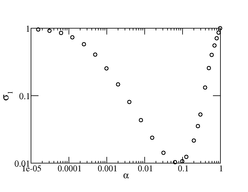
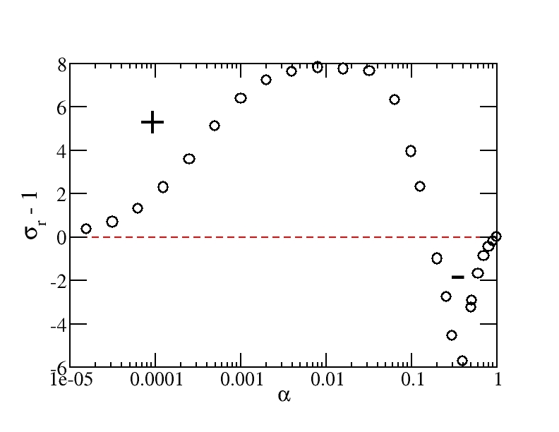
Figure 1: $\sigma_{1}$ and $\sigma_{r}-1$ as a function of $\alpha$ as obtained from the numerical simulations in 3D. $\sigma_{r}-1=0$ is highlighted by the broken line.

We start by showing $\sigma_{1}(\alpha)$ and $\sigma_{r}(\alpha)$ for the 3D case; see Fig.1. In the limits $\alpha\rightarrow 0$ and $\alpha\rightarrow 1$ the linear conductivity is identical because the particle is hopping in an energy landscape without any disorder. With the chosen normalization this conductivity equals unity. The conductivity is reduced by two orders of magnitude for intermediate $\alpha$ with a minimum around $\alpha\approx 0.1$. Qualitatively, the decrease of $\sigma_{1}$ for small $\alpha$ is related to the fact that the number of deep-lying traps is increasing which slows down the particle. In contrast, when approaching $\alpha=1$ from below, the residual high-energy states work as barriers, slowing down the dynamics. Since the fraction of high-energy states decreases for increasing $\alpha$ the conductivity increases correspondingly. The minimum reflects a crossover between the trap-regime and the barrier-regime.

Also the nonlinear conductivity as expressed via $\sigma_{r}$, i.e. the ratio of the nonlinear and the linear conductivity, displays two distinct regimes. Since for $\alpha=0$ and $\alpha=1$ one has $\sigma_{r}=1$ by construction, we discuss the behavior of $\sigma_{r}-1$ in the following. Interestingly in the trap-dominated regime one has $\sigma_{r}-1>0$, i.e. an increase of the nonlinearity as compared to the homogeneous case. In contrast, in the barrier-dominated regime we find $\sigma_{r}-1<0$ so that the nonlinearity is smaller. A physical understanding of these observations will be developed in the remaining part of this work. The simulations for higher dimensions display the same qualitative features.

IV Analytical results

In our analytical calculations we always consider the case of high but finite dimensions, expressed via $\Theta\gg 1$.

IV.1 Rate equations for a single low-energy site

We start with the case of a single low-energy state. This low-energy state as well as its direct neighbors are sketched in Fig.2. This region will be denoted trap-region.

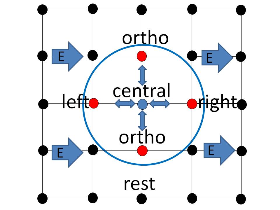
Figure 2: Sketch of the notation used in the main text. If the central site is a rare low-energy site $(\alpha\ll 1/\Theta$) local thermodynamic equilibrium is generated, motivating the notion of a trap-region with a border (circle).

For setting up a set of rate equations we assume that all sites adjacent to the trap-region possess the same non-equilibrium population $q_{rest}$ which, of course, depends on the applied field. Later one we argue that this assumption is not required and that it is sufficient in the limit of high dimensions to identify $q_{rest}$ with the average population. Then the rate equations read

$$(d/dt)q_{central} = -(1/Z)(y+1/y+\Theta)q_{central}+Z(yq_{left}+(1/y)q_{right}+\Theta q_{ortho}),$$ (2)

$$(d/dt)q_{ortho} = -(y+1/y+\Theta-1+Z)q_{ortho}+(y+1/y+\Theta-1)q_{rest}+(1/Z)q_{central},$$ (3)

$$(d/dt)q_{left} = -(Zy+1/y+\Theta)q_{left}+(y+\Theta)q_{rest}+(1/(yZ))q_{central},$$ (4)

$$(d/dt)q_{right} = -(Z/y+y+\Theta)q_{right}+(1/y+\Theta)q_{rest}+(y/Z)q_{central}.$$ (5)

In the stationary case the left side is zero so that one effectively obtains a system of four linear equations. In a first step one can obtain the general equation for $q_{central}$ and then after insertion solve for the other three populations. Whereas the general expression is too complex to directly extract relevant information we restrict ourselves to the limits $Z\gg\Theta$ and $Z\ll\Theta$. Since we always consider the case $\Theta\gg 1$ we express the final result as a linear expansion in $1/\Theta$.

IV.2 The limit of large disorder $Z\gg\Theta$ for $\alpha\Theta\ll 1$

We start by solving this set of equations, i.e. consider a single long-energy site. In the present case we have the two small parameters $1/\Theta$ and $\Theta/Z$. In practice we take the exact solution of this set of linear equations, expand this expression in powers of $1/Z$ and then, for fixed order $1/Z$, expand in $1/\Theta$. Finally, one keeps those up to linear order in $1/\Theta$ and $\Theta/Z$.

After a straightforward but somewhat lengthy calculation one obtains

$$q_{central} = c(y,Z)Z^{2}q_{rest},$$ (6)

$$q_{ortho} = \frac{1}{Z^{2}}q_{central},$$ (7)

$$q_{left} = \frac{y^{-2}}{Z^{2}}\left[1+\frac{\Theta}{Z}(y-y^{-1})\right]q_{central},$$ (8)

$$q_{right} = \frac{y^{2}}{Z^{2}}\left[1-\frac{\Theta}{Z}(y-y^{-1})\right]q_{central},$$ (9)

with

$$c(y,Z)=1-\frac{1}{\Theta}\frac{(y-y^{-1})^{2}}{f(y,Z)}.$$ (10)

where

$$f(y,Z)=1+\frac{\Theta}{Z}(y+y^{-1}-1).$$ (11)

The factor $f(y,Z)<1$ is close to unity and keeps track of corrections due to finite disorder as expressed by $Z$. Note that for finite field, i.e. $y\neq 1$, one obtains $c(y)<1$. This relation is of key importance for the subsequent discussion. Naturally, for vanishing external field, i.e. $y=1$, the Boltzmann populations are recovered.

Eqs.7-9 have a simple physical interpretation in the limit of large disorder, e.g. when the correction due to the $\Theta/Z$-term can be neglected. If a particle is sitting adjacent to a low-energy site the probability to jump to the low-energy site is by a factor of $Z/\Theta$ larger than to jump to one of the other $\Theta+1$ neighbor sites. Thus, many forward-backward jumps will occur between the low-energy site and its neighbors. As a consequence local thermodynamic equilibrium is generated around the central site which gives rise to the notation of a trap-region. The $y^{\pm 2}$-factors express that the external field attemps to shift the particle to the right. We mention in passing that this term has been also used in the work of Riess and Maier Riess and Maier (2009) about nonlinear conductivity, but with a very different meaning.

The factor of $c(y,Z)<1$ captures the absolute populations in the trap-region as compared to the population of the neighbors. As discussed in Appendix A its value (Eq.10) can be also rationalized via straightforward flux arguments.

The analysis, presented so far, was obtained under the additional assumption that all adjacent sites have the same population $q_{rest}$. Strictly speaking this is not true because the external field induces an anisotropic modification of the population. However, as discussed in Appendix B, this assumption can be relieved in the regime of high dimensions and $q_{rest}$ can be simply interpreted as the average population of the sites adjacent to the tagged region. Note that the types of sites, which allow one to obtain this conclusion, only exist for $d\geq 3$. Thus, one might expect that major deviations are present for $d=2$. It turns out (see Appendix B) that all higher-order terms in the expansion of $1/\Theta$ (starting with $1/\Theta^{2}$) would depend on the individual (unknown) populations. Exactly in the limit of high dimensions they can be neglected. This justifies that it is reasonable to stop the expansion in $1/\Theta$ after one term. Interestingly, already this first term captures many of the features, obtained for the numerical solution in 3D (see below).

Of particular relevance is the variation of the population of the central site $q_{central}=q_{rest}c(y,Z)Z^{2}$. Due to the factor $Z^{2}\gg 1$ even a small decrease of $c(y,Z)$ from unity gives rise to a significant decrease in population of the central site, i.e. particles less likely populate the low-energy site. This population difference has to be redistributed over the whole system, i.e. to the high-energy sites. We note in passing that this phenomenon resembles the Poole-Frenkel effect, albeit for different physical reasons Frenkel (1938). After escaping from the trap-region as a consequence of the external field these particles can now contribute to the total current. Since this population increase is induced by the external field, this effect contributes to the nonlinear response of the total system.

Now we generalize our analysis to a finite fraction $\alpha$ of low-energy sites. One can assume that they act independently if the probability that two low-energy sites are neighbors is small. Formally, this corresponds to $\alpha\Theta\ll 1$.

We choose the normalization such that the average population of a site is just unity, i.e. $(1-\alpha(3+\Theta))q_{rest}+\alpha(q_{central}+q_{left}+q_{right}+\Theta q_{ortho})=1$. In the limit of large $Z$ a straightforward evaluation of this expression together with Eqs.6-9 yields

$$q_{rest}=\frac{1}{1+c(y,Z)\alpha Z^{2}}.$$ (12)

After an expansion in $1/\Theta$ this can be rewritten as

$$q_{rest}=\frac{1}{1+\alpha Z^{2}}\left(1+\frac{\alpha Z^{2}}{\Theta(1+\alpha Z^{2})f(y,Z)}(y-1/y)^{2}\right).$$ (13)

The current (normalized per site), as generated by the sites beyond the trap-region is simply given by $q_{rest}(y-1/y)$. Furthermore, one can also calculate the contribution of the trap-regions. Although the population may be extremely high in this region it turns out that the current of the trap-region, i.e. $q_{left}(Zy-1/y)+q_{central}(y-1/y)/Z+q_{right}(y-Z/y)\propto\alpha q_{rest}Z^{0}$ is very small due to the factor of $\alpha$ and the missing factor of $Z$.

Inserting Eq.13 in the expression for the current and evaluation of the first-order and third-order terms in $w$ yields after a straightforward calculation (see Appendix C)

$$\sigma_{r}=1+\frac{\alpha Z^{2}}{(1+\alpha Z^{2}){f(y=1,Z)}}\frac{24}{\Theta}.$$ (14)

Naturally, for large $\Theta$ one recovers the mean-field limit $\sigma_{r}=1$.

IV.3 The limit of small disorder $Z\ll\Theta$ for $\alpha\ll 1/\Theta$

Using the same set of rate equations (Eq.2 to Eq.5) as in the previous case one directly performs an expansion in $1/\Theta$. One obtains after a straightforward calculation

$$q_{central} = Z^{2}q_{rest}+O(1/\Theta^{2}),$$ (15)

$$q_{ortho} = q_{rest}+O(1/\Theta^{2}),$$ (16)

$$q_{left} = [1-\frac{1}{\Theta}(y-1/y)(Z-1)]q_{rest},$$ (17)

$$q_{right} = [1+\frac{1}{\Theta}(y-1/y)(Z-1)]q_{rest}.$$ (18)

Note that in contrast to the limit of large disorder the total population in the trap-region is not changed upon application of an external field. In agreement with the previous case $q_{left}$ is somewhat decreased (because $Z>1$) whereas $q_{right}$ increases. In analogy to the limit of large disorder normalization leads to $q_{rest}=1/(1+\alpha(Z^{2}-1))$.

For the current, related to one left, one central and one right site one obtains after a short calculation $j_{left,center,right}=[(1+2Z)-(1/\Theta)(y+1/y)(Z-1)^{2}](y-1/y)q_{rest}$. The total current can be written as

$$j=\alpha j_{left,center,right}+(1-3\alpha)(y-1/y)q_{rest}.$$ (19)

This can be rewritten as

$$j=\frac{1+2\alpha(Z-1)}{1+\alpha(Z^{2}-1)}\left[1-\frac{1}{\Theta}\frac{\alpha(Z-1)^{2}}{1+2\alpha(Z-1)}(y+1/y)\right](y-1/y).$$ (20)

With a calculation in analogy to Appendix C one ends up with

$$\sigma_{r}(\alpha)=1-\frac{6}{\Theta}\frac{\alpha(Z-1)^{2}}{1+2\alpha(Z-1)}.$$ (21)

In contrast to strong disorder the nonlinearity decreases as compared to the homogeneous case. Qualitatively, this is due to the fact that upon increasing the external field intensity is shifted from the left to the right site. This shift of population decreases the total current because a particle on the right side is more likely shifted back to the central site and thus contributes with a negative sign.

IV.4 The limit $1-\alpha\ll 1/\Theta$

Here we deal with the limit that most sites are high-energy states. Actually, this limit is already implicitly contained in the previous calculation. The same approximations would have been valid if $0<Z<1$. If, for the moment, we interpret $\alpha$ as the number of high-energy states the value of $\sigma_{r}$ is again given by Eq.21. To keep the original notation we have to substitute $\alpha$ by $1-\alpha$ and $Z$ by $1/Z$ in Eq.21. This yields

$$\sigma_{r}(\alpha)=1-\frac{6}{\Theta}\frac{(1-\alpha)(Z-1)^{2}}{Z^{2}+2Z(1-\alpha)(1-Z)}.$$ (22)

Thus, independent of the degree of disorder one obtains a reduction of the nonlinearity if most states are low-energy states. The explanation is analogous to before, just the signs have to be reversed. To stress the qualitative picture one may imagine one inaccessible high-energy site. The external field pushes the particles in front of this site. Due to the inaccessibility the intensity $q_{left}$ is increased. Since, this left site cannot contribute to the current in field direction, there is an effective reduction in the total current.

IV.5 The general case except for the trap-regime

Here we introduce a very different approach for the high-dimensional case which is applicable for the whole parameter regime except for the trap-regime and is more general than the solutions, discussed above. The key idea is to use a statistical description which is as close to a mean field description (infinite $\Theta$) as possible but still reflects the properties of finite dimensions. Generally, two approximations reflect this limit. (1) After an orthogonal jump the previous site is randomly given a new energy based on the energy distribution, i.e. the memory on the previous site is lost. (2) For jumps along the field direction more information has to be included because these jumps determine the value of $\sigma_{r}$. Here the memory is lost after two successive jumps in one direction because then the backjump probability is proportional to $1/\Theta^{2}$.

This statistical picture is expected to break down in the case of a trap-regime ($\alpha\ll 1$ and $Z\gg\Theta$). Here after an orthogonal jump from a low-energy to a high-energy site it is essential to know that the previous site was a low-energy site because very likely the system will jump back. Within the statistical description, however, the backjump probability would be very small because the energy of the previous site would be determined according to the energy distribution which would, very likely, change the energy and thus suppress the trapping property.

The formal description, resulting from (1) and (2) requires the introduction of a probability $p_{ijk}$ that a particle sits on site $j\in\{+,-\}$ and has neighbor sites with energies $i$ and $k$ anti-parallel and parallel to the field direction, respectively ($i,k\in\{+,-\}$). Then the corresponding master equation reads

$$\dot{p}_{ijk} = \sum_{h}\alpha_{k}\,p_{hij}y\gamma_{ij}+\sum_{l}\alpha_{i}\,p_{jkl}\frac{1}{y}\gamma_{kj}+\Theta\,\alpha_{i}\alpha_{j}\alpha_{k}\left(\sum_{\tilde{i},\tilde{k}}p_{\tilde{i}-\tilde{k}}\gamma_{-j}+\sum_{\tilde{i},\tilde{k}}p_{\tilde{i}+\tilde{k}}\gamma_{+j}\right)$$ (23)

$$- p_{ijk}\left(y\gamma_{jk}+\frac{1}{y}\gamma_{ji}+\Theta\left(\alpha_{-}\gamma_{j-}+\alpha_{+}\gamma_{j+}\right)\right).$$

For the motivation of the individual terms we start by discussing the first term. The rate of jumping from site $i$ to site $j$ in the direction of the field is proportional to $p_{-ij}+p_{+ij}$, which is just the probability that two adjacent sites $(i,j)$ do exist. Since we want to calculate the change in the probability $p_{ijk}$ we also have to take into account that statistical factor $\alpha_{k}$ to have an adjacent site $k$. Furthermore a factor of $y$ keeps track of the direction of the jump. In summary, we obtain a contribution of $\sum_{h}\alpha_{k}\,p_{hij}y\gamma_{ij}$. To calculate the gain term after an orthogonal transition (third term) one has to keep into mind that the rate only depends on the energy difference of the old site (which was either plus or minus) and the energy of the new site $j$. Furthermore, the product $\alpha_{i}\alpha_{j}\alpha_{k}$ just expresses the probability to find three adjacent sites $(i,j,k)$. As discussed under point (1), no memory about the old site (plus or minus) is kept. The remaining terms can be derived analogously.

For the calculation of the stationary limit this corresponds to a set of 8 coupled linear equations. Again we perform a $1/\Theta$ expansion of the resulting population properties and, correspondingly, the resulting current. Here we just present the final result which we have checked by solving these equations by MAPLE. In lowest order of $1/\Theta$ the current reads

$$J(\alpha,w,Z,\Theta)=\frac{(1-\alpha+\alpha Z)^{2}}{1-\alpha+\alpha Z^{2}}\left[1-\frac{1}{\Theta}\,(y+1/y)\,\frac{\alpha(1-\alpha)(Z-1)^{2}}{(1-\alpha+\alpha Z)^{2}}\right](y-1/y).$$ (24)

This directly yields

$$\sigma_{r}(\alpha)\approx 1-\frac{1}{\Theta}\,6\,\frac{\alpha(1-\alpha)(Z-1)^{2}}{(1-\alpha+\alpha Z)^{2}}.$$ (25)

Most importantly, this general relation has Eq.21 and Eq.22 as limiting cases if choosing $\alpha\ll 1$ or $1-\alpha\ll 1$, respectively. As described above, the trapping picture cannot be described by this ansatz.

V Comparison of the numerical and the analytical results

The key results of this work deal with the limits $\alpha\Theta\ll 1$ or $\alpha\Theta\gg 1$ for the physical relevant limit of high disorder, i.e. $Z\gg\Theta$. In a first step we compare the numerical results for $d=3$ and $d=6$ for $\sigma_{1}$ and $\sigma_{r}$ with the analytical expressions in the respective limits. As before, we use $Z=\exp(4)$ and choose $\sigma_{r}-1$ for our comparison.

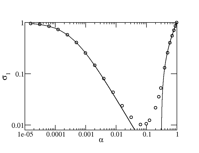
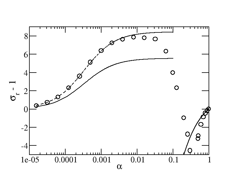
Figure 3: Squares: Numerical results for $\sigma_{1}(\alpha)$ (left) and $\sigma_{3}(\alpha)$ (right) for the 3D case. Solid lines: Analytical solutions for both the limits of small and large $\alpha$. The value of $Z$ is chosen as $\exp(4)$. Broken line: The analytical solution is scaled by a factor of 1.5.

The results for the 3D case are shown in Fig.3. The linear conductivity $\sigma_{1}$ is reproduced very well. Qualitatively, $\sigma_{r}-1$ is also reproduced for both limits of small $\alpha$ and large $\alpha$. Interestingly, when scaling the theoretical curve by a constant factor of 1.5 one achieves a perfect agreement between numerics and analytical theory for $\alpha\leq 2\cdot 10^{-3}$. This scaling property is just a consequence of the fact that in this regime the individual traps act independently. However, the fact that also the sigmoidal shape of $\sigma_{r}-1$ is reproduced clearly shows that the trap-mechanism, as discussed above, fully explains the nature of the nonlinear conductivity in the experimentally relevant 3D case. Also the $\alpha$-dependence for large $\alpha$, giving rise to negative $\sigma_{r}-1$, is reproduced. However, a quantitative comparison is only possible for $\alpha\geq 0.9$.

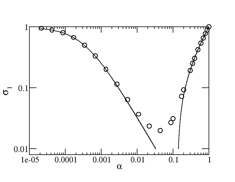
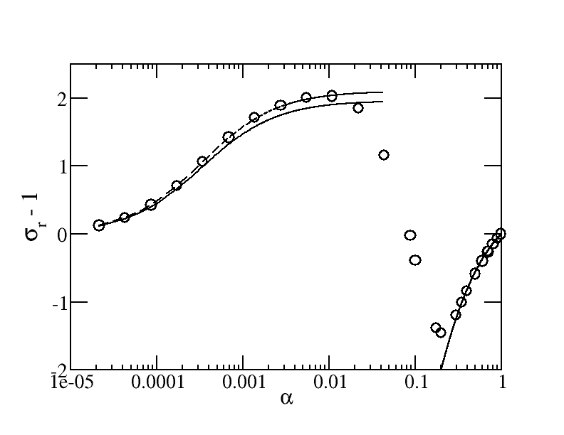
Figure 4: Same as the previous figure for the 6D case. The analytical solution is scaled by a factor of 1.08.

Next we compare the numerical and analytical results for $d=6$; see Fig.4. In agreement with the 3D case the linear conductivity is reproduced very well in both limits. The crossover regime has a similar size (one order of magnitude on the $\alpha$-scale) but is shifted to somewhat lower $\alpha$-values. This is to be expected because the crossover should scale like $1/\Theta$. Most remarkable, the agreement for the non-linearity $\sigma_{r}-1$ is very good. The trap-regime is fully reproduced, and the remaining scaling factor is reduced from 1.5 in 3D to 1.08 in 6D. This improvement does not come as a surprise because the analytical theory should be particulary good for high dimensions. A dramatic improvement as compared to the 3D case is observed for the barrier-regime. Here a quantitative agreement is seen for $\alpha$ as small as 0.3. Obviously, the neglect of back-jump memory is by far more justified for the 6D than for the 3D case.

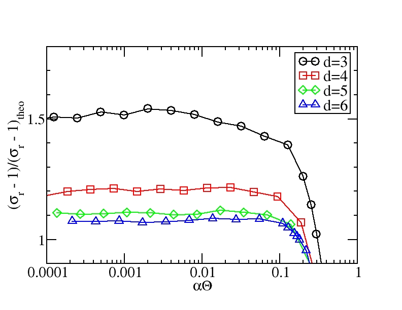
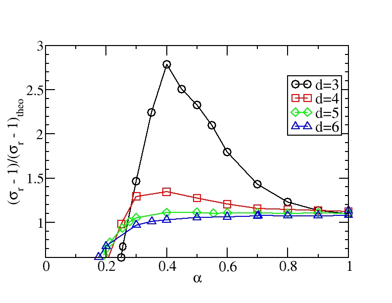
Figure 5: The ratio of the actual numerical and the approximate theoretical value of $(\sigma_{r}-1)$ for small $\alpha$ (left) and large $\alpha$ (right). The lines serve as a guide for the eyes.

For both dimensions we observe that the breakdown of the theoretical expectation for $\sigma_{1}$ and $\sigma_{r}$ in the trap-regime occurs at very similar values of $\alpha$ (3D: $\alpha\approx 0.04$; 6D: $\alpha\approx 0.02$). We checked that the same holds if we directly compare $\sigma_{3}$ with the theoretical expectation. Thus, the range of applicability of the linear and nonlinear prediction is very similar.

Finally, we compare the ratio of the actual numerical and the approximate theoretical value of the nonlinearity parameter $(\sigma_{r}-1)$; see Fig.5. This representation highlights the results, discussed in Figs.3 and 4 and, furthermore, allows one to see the gradual increase of predictability when going beyond the 3D case. In the trap-regime (small $\alpha$) we compare the different dimensions as a function of the scaled variable $\alpha\Theta$. It turns out that for all dimensions a plateau-value emerges. As discussed above this implies the relevance of the trap-picture for all dimensions. The plateau-value strongly depends on the dimension and approaches one for high dimensions. As discussed before, these deviations reflect that quality of the approximation that $q_{rest}$ can be identified with the average population. It becomes good for high dimensions. Interestingly, in all cases the plateau-behavior breaks down for $\alpha\Theta\approx 0.1$. As mentioned above, the presence of non-adjacent low-energy states and thus the applicability of the analytical approach in the trap-regime was related to the inequality $\alpha\Theta\ll 1$. In the opposite case, i.e. in the barrier-regime, the analytical prediction is good for $\alpha\geq 0.3$ except for the 3D case where the prediction already fails for $\alpha<0.8$. As expected from the range of validity of the underlying approach, the breakdown of this approximation is related to $\alpha$ rather than $\alpha\Theta$, at least for $d\geq 4$.

We also performed simulations in the limit $1\leq Z\leq\Theta$ and $\alpha\Theta\ll 1$, as reflected by Eq.21. Although the qualitative features, in particular a negative $\sigma_{r}-1$, can be reproduced, a quantitative comparison requires very high dimensions which are beyond the scope of our computer simulations.

VI Discussion

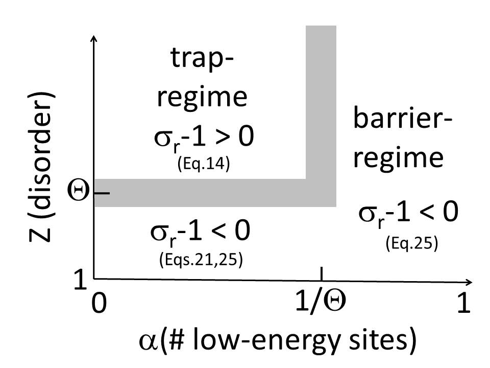
Figure 6: The nonlinear response in dependence of $\alpha,Z$ and $\Theta$ as discussed in this work.

In this work we have described the nonlinearity for a simple lattice model with a bimodal energy distribution in dependence of the fraction of low-energy sites $\alpha$, the disorder (via $Z$) and the dimension (via $\Theta$). A clear physical picture is presented for the limits of a small number ($\alpha\ll 1/\Theta$) and a large number ($1-\alpha\ll 1$) of low-energy states in the limit of large disorder ($Z\gg\Theta)$; see Fig.6 for a sketch of the whole $\alpha,Z$-phase space. In the first case the few low-energy states serve as traps which are in a local thermodynamic equilibrium-state with the adjacent sites. This gives rise to a reshuffling of intensity to the high-energy states so that the positive nonlinear contribution is via the nonlinear increase of the current of the high-energy states, i.e. $\sigma_{r}>1$. In the other limit of many low-energy states the remaining high-energy states serve as barriers which accumulate intensity on the neighbor site opposite to the field direction and decreases the intensity on the adjacent site parallel to the field direction, respectively. The contribution to the total current, however, has the reverse order. Thus, one obtains an effective decrease of the non-linear conductivity, i.e. $\sigma_{r}<1$.

Note that for sufficiently large $Z$ there exists a regime where $\sigma_{r}=1+24/\Theta$ does not depend on $\alpha$ ($1\ll\alpha Z^{2}$). Whereas this theoretical plateau value is close to the numerical value for higher dimensions, a difference of a factor of 1.5 is observed for the 3D case (see Fig.3). Furthermore, in this limit also the $Z$-dependence is very weak (only via $f(y,Z)$) and disappears for large $Z$. We mention in passing that also the 2D model displays a plateau value. However, here the numerical value is even two times higher than the theoretical value (data not shown).

For large disorder the theoretical predictions are not applicable in the regime $0.1<\alpha\Theta<2.5$ (see Fig.5). Note that the critical value $\alpha_{c}$ for site percolation for high dimensions is approximately $1/\Theta$ (e.g. $\alpha_{c}(d=13)\approx 1.025/\Theta$ Grassberger (2003)). It is known that above the percolation threshold the linear conductivity strongly increases because the particles can cross the sample without using the high-energy states. The present results show that also the nonlinear conductivity shows a significant change around this critical concentration of low-energy sites. However, a closer relation of the crossover-regime to the percolation approach is beyond the scope of this work.

From a theoretical perspective one might want to consider more complex energy distributions. Although the general physical mechanisms, described in this work, may remain the same, a quantitative analysis would become much more difficult if not intractable within the present approach. E.g., the analysis of a model with three instead of two different energy levels in the barrier-regime would require the solution of 27 instead of 8 linear equations. Nevertheless, the insight of the present work on the two-state model can be used to rationalize the numerical results, previously obtained for hopping models with continuous energy distributions (see Introduction). For a Gaussian distribution the resulting nonlinearity was analyzed in dependence on the lowest energy $U_{min}$ of all sites Röthel et al. (2010). Among the different realizations of the Gaussian random numbers the value of $U_{min}$ fluctuates quite significantly. It turned out that (1) only for sufficiently low values of $U_{min}$ one indeed observes $\sigma_{r}>1$ whereas otherwise one has $\sigma_{r}<1$ and (2) in the regime of sufficiently low values of $U_{min}$ (i.e., $\sigma_{r}>1$) the value of $\sigma_{r}$ hardly depends on the specific value of $U_{min}$ Röthel et al. (2010). Both observations can be qualitatively explained by the present results. Due to the dependence on the single low-energy value $U_{min}$ the continuous distribution can be related to a discrete model with one particular low-energy state. Qualitatively, this corresponds to the present bimodal model in the trap-regime. If $\Delta U$ is too small one indeed observes $\sigma_{r}<1$ because local equilibration does not occur and the nonlinearity is explained via the barrier-mechanism. Furthermore, for large $Z$ no dependence on the disorder is observed (explanation of observation(2)). Thus, several non-trivial observations from a continuous Gaussian distribution can be rationalized by the insights from the bimodal model. In previous simulations also the box-type distribution was analysed somewhat closer. It was shown that in this case one observes $\sigma_{r}<1$ Röthel et al. (2010). When mapping this distribution on a bimodal distribution an appropriate choice is $\alpha\approx 1/2$. Here we obtain $\sigma_{r}<1$ in agreement with the numerical result.

The rate equations Eq.2 to Eq.5 required implementation of the approximation that the population of all neighbor sites is identical. Although we found a strict argument why this approximation is not required for the validity of our approach, it is promising that the general approach Eq.23 yields identical results for the limits $1-\alpha\ll 1/\Theta$ as well as $\alpha\ll 1/\Theta$ together with $Z\ll\Theta$. This serves as an important consistency check of the two complementary approaches, used in this work.

As outlined in the Introduction hopping models constitute a reasonable approach for the real-world situation in inorganic ion conductors. The previous numerical results indicated that the experimental observation $\sigma_{r}>1$ suggests a very broad distribution of the site energies such that there exist a few sites with very low energies Röthel et al. (2010). However, in the previous work no physical picture for this observation could be supplied. The present work suggests that the presence of these low-energy sites gives rise to the phenomenon of local thermodynamic equilibrium which is responsible for the experimental observation $\sigma_{r}>1$. Please note that the terminology of sites was related to the vacancy picture. Going back to the ion rather than the vacancy picture the positive nonlinear effect translates into the presence of a few unfavorable sites which nevertheless have to be frequently visited by the ion due to the shortage of vacant sites.

In summary, to the best of our knowledge we have for the first time formulated quantitative predictions for the non-linear response of a disordered hopping model in high dimensions with several predictions which semi-quantitatively already hold for the experimentally relevant 3D case and hold very well for even higher dimensions. Thus, the experimentally observed positive nonlinear effect indicates the presence of strong disorder with only a few sites with very low energy as outlined for the case of the Gaussian distribution. A more direct experimental analysis of non-linear single-particle dynamics is possible with modern holographic-mechanical optical tweezers Hanes et al. (2009); Dalle-Ferrier et al. (2011) which can generate random potentials and may allow for a more quantitative comparison with the dynamics in disordered energy landscapes.

We acknowledge very helpful discussions with B. Roling, S. Röthel, T. Franosch, and S. Egelhaaf about this project. In particular we would like to acknowledge the very fruitful collaboration with our late colleague R. Friedrich on the topic of this work. We gratefully acknowledge the financial support by the DFG via FOR 1348 and SFB 458.

Appendix A

Here we present an alternative argument for Eq.10 in the limit $\Theta/Z\rightarrow 0$. In the stationary non-equilibrium case the total fluxes in and out of the trap-region have to be identical. Counting the number of possible transitions the flux balance can be written as

$$q_{left}(\Theta+1/y)+q_{right}(\Theta+y)+q_{ortho}\Theta(\Theta+y+1/y-1)=q_{rest}(\Theta^{2}+\Theta(y+1/y+1)+y+1/y)$$ (26)

Neglecting the terms of order $\Theta^{0}$ and using Eqs.7-9 (without the correction terms of order $\Theta/Z$) this can be rewritten as

$$(y^{-2}+y^{2}-2+y+1/y+1+\Theta)q_{ortho}=(y+1/y+1+\Theta)q_{rest}$$ (27)

which after expansion in $1/\Theta$ and comparison with Eq.7 directly yields Eq.10 (again without the correction terms). Thus, the factor $c(y,Z)<1$ balances the increase of intensity of $q_{left}+q_{right}$, following from $y^{2}+y^{-2}>2$ for $y>1$.

Appendix B

Here we show that for the derivation of the leading term of $c(y)$ it does not matter whether the populations of the sites, adjacent to the trap-region, are identical or not. Using a vector notation we choose the central site as $(0,...,0)$, the left and right sites as $(\pm 1,0,..,0)$ and the orthogonal sites as $(0,...,\pm 1,...)$. Coordinates different from zero are explicitly listed .Then the neighbors of the trap-region can be classified into six types: (1) $(0,...,\pm 1,...,\pm 1,...)$, (2) $(0,...,\pm 2,...)$, (3) $(+1,...,\pm 1,...)$, (4) $(-1,...,\pm 1,...)$, (5) $(+2,...)$, (6) $(-2,...)$. Within one type all populations are identical due to symmetry reasons. The individual populations are denoted $q_{i}$ with $i\in{1,...,6}$. The number of sites $n_{i}$ can be easily calculated. It turns out that only $n_{1}$ is of order $\Theta^{2}$ (namely $n_{1}=(1/2)\Theta^{2}-\Theta$) whereas all other $n_{i}$ are at most of order $\Theta$ $(n_{2}=n_{3}=n_{4}=\Theta,n_{5}=n_{6}=1)$ . The total number of sites $n_{tot}$ is $(1/2)\Theta^{2}+2\Theta+2$. Denoting $q_{rest}$ as the average population of a site one has the simple relation

$$\sum_{i=1}^{6}n_{i}q_{i}=n_{tot}q_{rest}.$$ (28)

In the mean-field limit $\Theta\rightarrow\infty$ one can write $q_{i}=q_{rest}$ because the Boltzmann probabilities are recovered. For finite but large dimension one can choose the expansion ansatz $q_{i}=q_{rest}(1+a_{i}/\Theta+b_{i}/\Theta^{2}+...)$ where, again, $q_{rest}$ denotes the average population of all sites. Inserting this ansatz into Eq.28 and comparing all terms of order $\Theta$ one immediately obtains $a_{1}=0$. Thus, in case of symmetry breaking the impact of finite order on $q_{1}$ is only of order $1/\Theta^{2}$.

Going back to the rate equations Eq.2 to Eq.5 one has to modify the source terms by replacing $q_{rest}$ by the specific populations $q_{i}$, defined above. After a straightforward calculation one realizes that for the relevant orders in $\Theta$ only the term $a_{1}$ would contribute which, however, is zero. Thus, all variations of $q_{i}$ from $q_{rest}$ are irrelevant for the first order expansion in $1/\Theta$ and would only show up in the higher-order terms.

Of course, the above arguments can be also applied for the next shell of sites around the sites considered above. Again, there is one type of sites which dominates all other sites in the limit of high dimensions. Reiterating this argument one can conclude that $q_{rest}$ can be even identified with the average population of all sites of the system beyond the tagged region if one restricts oneself to the corrections of order $1/\Theta$.

We mention in passing that for the 2D case ($\Theta=2$) one has $n_{1}=0$. Thus, the key states for argumentation only start to exist for $d=3$ and a quantitative comparison for the 2D case should be quite poor. This is indeed reflected by the actual comparison as indicated in the main text.

Appendix C

For the calculation of the nonlinear conductivity in Sect. IV B we start with the relation

$$q_{rest}\propto\left(1+k(y-1/y)^{2}\right).$$ (29)

with

$$k=\frac{\alpha Z^{2}}{\Theta(1+\alpha Z^{2})}.$$ (30)

The current $j$ is given by $(y+1/y)q_{rest}\propto(w+w^{3}/6)q_{rest}$. Up to third order in $w$ one can write (using $y=\exp(w)$)

$$j\propto(w+w^{3}/6)(1+k(2w)^{2})\propto w(1+(4k+1/6)w^{2}).$$ (31)

This immediately yields Eq.14.

References

- Croce et al. (1998) F. Croce, G. B. Appetecci, L. Persi, and B. Scrosati, Nature 400, 1998 (1998).
- Noda et al. (2004) K. Noda, T. Yasuda, and Y. Nishi, Electrochim. Acta 50, 2004 (2004).
- Isard (1996) J. O. Isard, J. Non-Cryst. Solids 202, 137 (1996).
- Murugavel and Roling (2005) S. Murugavel and B. Roling, J. Non-Cryst. Solids 351, 2819 (2005).
- Staesche and Roling (2010a) H. Staesche and B. Roling, Phys. Rev. B 82, 134202 (2010a).
- Ingram (1987) M. D. Ingram, Phys. Chem. Glasses 28, 215 (1987).
- Dyre et al. (2009) J. C. Dyre, P. Maass, B. Roling, and D. L. Sidebottom, Rep. Prog. Phys. 72, 046501 (2009).
- Maass (1999) P. Maass, J. Non-Cryst. Solids 255, 35 (1999).
- Banhatti and Funke (2006) R. D. Banhatti and K. Funke, Solid State Ionics 177, 1551 (2006).
- Hunt (1991) A. G. Hunt, J. Phys. Cond. Mat. 3, 7831 (1991).
- Baranovskii and Cordes (1999) S. D. Baranovskii and H. Cordes, J. Chem. Phys. 111, 7546 (1999).
- Dyre and Schrøder (2000) J. C. Dyre and T. B. Schrøder, Rev. Mod. Phys. 72, 873 (2000).
- Schrøder and Dyre (2008) T. B. Schrøder and J. C. Dyre, Phys. Rev. Lett. 101, 025901 (2008).
- Lammert and Heuer (2010) H. Lammert and A. Heuer, Phys. Rev. Lett. 104, 125901 (2010).
- Kunow and Heuer (2006) M. Kunow and A. Heuer, J. Chem. Phys. 124, 214703 (2006).
- Ambegaokar and Halperin (1969) V. Ambegaokar and B. I. Halperin, Phys. Rev. Lett. 22, 1364 (1969).
- B.Derrida (1983) B.Derrida, J. Stat. Phys. 31, 433 (1983).
- J.P.Bouchaud and A.Georges (1990) J.P.Bouchaud and A.Georges, Phys. Rep. 195, 127 (1990).
- Khoury et al. (2011) M. Khoury, A. M. Lacasta, J. M. Sancho, and K. Lindenberg, Phys. Rev. Lett. 106, 090602 (2011).
- Kehr et al. (1997) K. W. Kehr, K. Mussawisade, T. Wichmann, and W. Dieterich, Phys. Rev. E 56, R2351 (1997).
- Heuer et al. (2005) A. Heuer, S. Murugavel, and B. Roling, Phys. Rev. B 72, 174304 (2005).
- Eimax et al. (2008) M. Eimax, M. Koerner, P. Maass, and A. Nitzan, Phys. Chem. Chem. Phys. 12, 645 (2008).
- Dierl et al. (2012) M. Dierl, P. Maass, and M. Einax, Phys. Rev. Lett. 108, 060603 (2012).
- Roling et al. (2008) B. Roling, S. Murugavel, A. Heuer, L. Lühning, R. Friedrich, and S. Röthel, Phys. Chem. Chem. Phys. 10, 4211 (2008).
- Lubashevsky et al. (2009) I. Lubashevsky, R. Friedrich, A. Heuer, and A. Ushakov, Physica A 388, 4535 (2009).
- Marianer and Shklovskii (1992) S. Marianer and B. Shklovskii, Phys. Rev. B 46, 13100 (1992).
- Jansson et al. (2008) F. Jansson, S. Baranovskii, F. Gebhard, and R. Oesterbacka, Phys. Rev. B 77, 195211 (2008).
- Boettger and Bryksin (1985) H. Boettger and V. Bryksin, Hopping Conduction in Solids (VCH, New York, 1985).
- Riess and Maier (2008) I. Riess and J. Maier, Phys. Rev. Lett. 100, 205901 (2008).
- Staesche and Roling (2010b) H. Staesche and B. Roling, Z. Phys. Chem. 224, 1655 (2010b).
- Lammert et al. (2003) H. Lammert, M. Kunow, and A. Heuer, Phys. Rev. Lett. 90, 215901 (2003).
- Röthel et al. (2010) S. Röthel, R. Friedrich, L. Lühning, and A. Heuer, Z. Phys. Chem. 224, 1855 (2010).
- Heuer and Silbey (1993) A. Heuer and R. J. Silbey, Phys. Rev. Lett. 70, 3911 (1993).
- Heuer (1998) A. Heuer, Tunneling Systems in Amorphous and Crystalline Solids (ed. by P. Esquinazi) (Springer-Verlag, 1998), chapter 8.
- Riess and Maier (2009) I. Riess and J. Maier, J. Electrochem. Soc. 156, P7 (2009).
- Frenkel (1938) J. Frenkel, Phys. Rev. 54, 647 (1938).
- Grassberger (2003) P. Grassberger, Phys. Rev. E 672, 036101 (2003).
- Hanes et al. (2009) R. Hanes, M. Jenkins, and S. Egelhaaf, Rev. Sci. Instrum. 80, 083703 (2009).
- Dalle-Ferrier et al. (2011) C. Dalle-Ferrier, M. Krueger, R. D. L. Hanes, S. Walta, M. C. Jenkins, and S. U. Egelhaaf, Soft Matter 7, 2064 (2011).