THE PROPERTIES OF  EMISSION-LINE GALAXIES AT $z$ = 2.24^†

Abstract

Using deep narrow-band $H_{2}S1$ and $K_{\rm s}$-band imaging data obtained with CFHT/WIRCam, we identify a sample of 56  emission-line galaxies (ELGs) at $z=2.24$ with the 5$\sigma$ depths of $H_{2}S1=22.8$ and $K_{\rm s}=24.8$ (AB) over 383 arcmin² area in the Extended Chandra Deep Field South. A detailed analysis is carried out with existing multi-wavelength data in this field. Three of the 56  ELGs are detected in Chandra 4 Ms X-ray observations and two of them are classified as active galactic nuclei. The rest-frame UV and optical morphologies revealed by HST/ACS and WFC3 deep images show that nearly half of the  ELGs are either merging systems or have a close companion, indicating that the merging/interacting processes play a key role in regulating star formation at cosmic epoch $z=2-3$; About 14% are too faint to be resolved in the rest-frame UV morphology due to high dust extinction. We estimate dust extinction from spectral energy distributions. We find that dust extinction is generally correlated with  luminosity and stellar mass. Our results suggest that  ELGs are representative of star-forming galaxies. Applying extinction corrections for individual objects, we examine the intrinsic  luminosity function (LF) at $z=2.24$, obtaining a best-fit Schechter function characterized by a faint-end slope of $\alpha=-1.3$. This is shallower than the typical slope of $\alpha=\sim-1.6$ in previous works based on constant extinction correction. We demonstrate that this difference is mainly due to the different extinction corrections. The proper extinction correction is thus the key to recovering the intrinsic LF as the extinction globally increases with  luminosity. Moreover, we find that our  LF mirrors the stellar mass function of star-forming galaxies at the same cosmic epoch. This finding indeed reflects the tight correlation between star formation rate and stellar mass for the star-forming galaxies, i.e., the so-called main sequence.

1. INTRODUCTION

The cosmic star formation rate (SFR) density peaks at $z\sim 2-3$ and rapidly declines to the present day (Hopkins & Beacom, 2006; Karim et al., 2011; Sobral et al., 2013, and references therein). Systematic studies of galaxy populations at the peak epoch hold the key to our understanding of galaxy formation and evolution, in particular for massive galaxies. The population of massive quiescent galaxies began to emerge (e.g., Brammer et al., 2011) and the bulk of stars in local massive galaxies were formed at $z>\sim 1.5$ (Renzini, 2006). A number of techniques have been developed to probe different galaxy populations in this crucial epoch, including Lyman break selection (Steidel et al., 1999), red color cut (Franx et al., 2003), $BzK$ selection (Daddi et al., 2004), submillimeter detection (Chapman et al., 2005) and narrow-band imaging (Moorwood et al. 2000; see Shapley 2011 for a review). A complete picture is still missing due to the short of spectroscopic follow ups in the “redshift desert” $1.4<z<2.5$ for large samples selected in terms of physical quantities such as stellar mass or SFR.

The deep near-infrared (NIR) observations play a central role in probing high-$z$ galaxies in the rest-frame optical, which is more reflective of older stars (hence stellar mass). The NIR narrow-band imaging has turned out to be a modest way to identify emission-line galaxies (ELGs) in a narrow redshift range ($\delta z/(1+z)=1\%-2$%) over large sky coverage (Sobral et al., 2013). It provides redshifts with higher precision than the photometric redshift method based on broad-band spectral energy distributions (SEDs), and allows us to distinguish environments (e.g., groups or clusters) traced by the ELGs (e.g., Matsuda et al., 2011; Hatch et al., 2011; Geach et al., 2012). Moreover, the strength of an emission line, such as  and [O II]$\lambda$3727, can be measured by the flux excess in the narrow-band with respect to the corresponding broad-band. The optical and NIR emission lines from ionized gas surrounding massive young stars represent a nearly instantaneous measure of the SFR (Kennicutt & Evans, 2012). The  is often used as an SFR indicator because it is the strongest emission line in the optical/NIR, and less affected by dust obscuration compared to emission lines in the UV such as Ly$\alpha$ in typical star-forming galaxies (SFGs).

The past decade has seen a number of NIR narrow-band surveys using ground-based telescopes (e.g., Geach et al., 2008; Ly et al., 2011) and NIR grism spectroscopic surveys with the Hubble Space Telescope (HST; e.g., Yan et al., 1999; Atek et al., 2010; van Dokkum et al., 2011; Colbert et al., 2013) in the study of  ELGs at $z>$0.4, yielding  luminosity functions (LFs) with a steep faint-end slope $\alpha\sim-1.6$ out to $z\sim 2.5$ (Hayes et al., 2010; Ly et al., 2011; Sobral et al., 2013). The derived  LFs suffer from large uncertainties mostly arising from poor extinction correction due to the lack of ancillary data. Detailed studies of the properties of  ELGs will help to reduce the uncertainties. On the other hand, SFGs are found to follow a tight correlation between SFR and stellar mass (e.g., Noeske et al., 2007; Daddi et al., 2007). This correlation, namely the main sequence, has been convincingly established from the local universe (Brinchmann et al., 2004) to high-redshift universe (Guo et al., 2013; Peng et al., 2010; Karim et al., 2011; Reddy et al., 2012). One would expect that the SFR function traces the stellar mass function (SMF) for SFGs. Since  luminosity is a direct measure of SFR, the  LF is expected to mirror the SMF. However, the SMF tends to have a shallow faint-end with a slope $\alpha\sim-1.3$ over a wide redshift range $0<z<3$ (e.g., Ilbert et al., 2010; Brammer et al., 2011). The cause of this discrepancy in the faint-end slope between the two functions remains to be explored.

We carry out a deep 2.13 $\micron$ narrow-band imaging survey to search for  ELGs at $z$ = 2.24 in the Extended Chandra Deep Field South (ECDFS). This field contains the deepest observations from Chandra, Galaxy Evolution Explorer, HST, and Spitzer. With these data, we are able to securely identify a sample of  ELGs, perform a detailed analysis and determine the intrinsic  LF. We show that resolving dusty SFGs with intrinsically luminous  from those with observed faint  leads to a shallow faint-end slope for the  LF. We describe observations and data reduction in Section 2. Section 3 gives the selection of  ELGs and SED analysis to obtain photometric redshift, stellar mass and extinction. We present the properties of  ELGs in Section 4. The derived  LF at $z=2.24$ is given in Section 5. We discuss and summarize our results in Section 6. Throughout the paper we adopt a cosmology with [$\Omega_{\Lambda}$, $\Omega_{M}$, $h_{70}$] = [0.7, 0.3, 1.0]. Kroupa initial mass function (IMF; Kroupa, 2001) and the AB magnitude system (Oke, 1974) are used unless otherwise stated.

2. OBSERVATIONS AND DATA REDUCTION

The deep narrow-band imaging of the ECDFS ($\alpha$ = 03:28:45, $\delta$ = $-$27:48:00) were taken with WIRCam on board the Canada-France-Hawaii Telescope (CFHT; Puget et al., 2004) through the $H_{2}S1$ filter ($\lambda_{\mathrm{c}}=2.130\,\micron$, $\Delta\lambda=0.0293$ $\micron$). WIRCam is equipped with four 2048$\times$2048 HAWAII2-RG detectors, providing a field of view 20$\arcmin\times 20\arcmin$ and a pixel scale of 0$\farcs$3  pixel^-1. The gaps between detectors are 45$\arcsec$. The $H_{2}S1$ observations were carried out under seeing conditions of 0$\farcs$6$-0\farcs$8 with a total integration time of 17.22 hrs in semester 2011B. Dithering technique was adopted in observations in order to remove bad pixels and cover gaps between detectors.

The data were reduced using the pipeline SIMPLE (Simple Imaging and Mosaicking Pipeline) written in IDL (Wang et al., 2010; Hsieh et al., 2012), which include flat-fielding, background subtraction, removing cosmic rays, and instrumental features like crosstalk and residual images from saturated objects in previous exposures and masking satellite trails. Because of the rapid variation of sky background in the NIR, only exposures taken in the same dithering block (within 40 minutes) and by the same detector are reduced in the same run and combined into a background-subtracted science image. After that, the science images of four detectors are mosaicked into a frame science image. The $H_{2}S1$ images are astrometrically calibrated with the HST observations from the Galaxy Evolution from Morphology and SEDs (GEMS; Rix et al., 2004; Caldwell et al., 2008) survey using a list of 7415 compact sources with $K_{\mathrm{s}}<21.5$. The accuracy of astrometry is $\sim 0\farcs$1. The final science image was produced by co-adding 326 frame science images. The exposure time map was also created in the co-adding. The photometric calibration is performed with the $K_{\mathrm{s}}$-band photometric catalog of the Great Observatories Origins Deep Survey (GOODS) South extracted from VLT/ISAAC observations (Retzlaff et al., 2010). In total 125 point sources with $16.0<K_{\mathrm{s}}<19.0$ are chosen as photometric standard stars used to build empirical point spread function (PSF). A correction of 1.26 is derived from the empirical PSF to convert a flux integrated within an aperture of diameter of 2$\arcsec$ into the total flux. The calibrated fluxes of the chosen point sources in our mosaic $H_{2}S1$ image only show 1% scatter compared with these given in the reference catalog. The final $H_{2}S1$ science image has 383 arcmin² area with a total integrated exposure time $>10$ hr (and $>15$ hr for 47.3%). We limited source detection in this area, where a 5$\sigma$ depth corresponds to 22.8 mag for point sources.

We also utilize $K_{\mathrm{s}}$-band ($\lambda_{\mathrm{c}}=2.146\,\micron$, $\Delta\lambda=0.325\,\micron$) imaging of ECDFS obtained with CFHT/WIRCam (Hsieh et al., 2012). The $K_{\mathrm{s}}$-band observations were taken with CFHT/WIRCam in semesters 2009B and 2010B. The data were reduced and calibrated in the same way as we describe above for the $H_{2}S1$ data. The $K_{\mathrm{s}}$ image reaches a 5$\sigma$ depth of $K_{\mathrm{s}}$ = 24.8 mag for point sources in the $H_{2}S1$ source detection region. More technical details can be found in Wang et al. (2010) and Hsieh et al. (2012). The 5$\sigma$ limit for extended sources with a Sérsic index of unity is 0.4 mag lower for the $H_{2}S1$ image and 0.3 mag lower for the $K_{\mathrm{s}}$ image.

3. SAMPLE SELECTION

3.1. Selection of Emission-line Objects

We use SExtractor software (Bertin & Arnouts, 1996) to detect sources and measure fluxes in the $H_{2}S1$ image. A minimum of five contiguous pixels with fluxes $>2.5\sigma$ of the background noise is required for a secure source detection. The exposure map is taken as weight image to reduce spurious detections in low signal-to-noise (S/N) regions. The “dual-image” mode in SExtractor is used to perform photometry in the $K_{\mathrm{s}}$ image, namely, to measure fluxes in the $K_{\mathrm{s}}$ image over the same area of a detection as in the $H_{2}S1$ image. Of course, the two images are well aligned into the same frame. In total , 8720 sources are securely detected with an S/N $>5$ in both images.

As we have stated in Section 1, the narrow-band excess is an emission-line indicator that is widely used to identify emission-line objects. Here we use $K_{\rm s}-H_{2}S1$ to probe  emission-line objects following Bunker et al. (1995). A secure and significant narrow-band excess is mainly determined by the background noises of the narrow- and broad-band images $\sigma_{\rm H_{\mathrm{2}}S1}$ and $\sigma_{K_{\rm s}}$ as follows:

$$K_{\rm s}-H_{\mathrm{2}}S1>\Sigma\sqrt{\sigma_{K_{\rm s}}^{2}+\sigma_{\rm H_{\mathrm{2}}S1}^{2}},$$ (1)

where the right-hand side term is the combined background noise of the two bands and $\Sigma$ is the significant factor. Figure 1 shows the $K_{\rm s}-H_{2}S1$ color as a function of $H_{2}S1$ magnitude for 8720 sources. The solid curve represents the combined noise with $\Sigma$ = 3 and the dotted curve refers to the noise with $\Sigma$ = 2. We adopt $\Sigma>3$ to select emission-line candidates. In order to minimize false excess caused by photon noises of bright objects, we also employ an empirical cut EW $>50$ Å following Geach et al. (2008), where EW refers to the rest-frame equivalent width of an emission line. This cut corresponds to $K_{\rm s}-H_{\mathrm{2}}S1>0.39$ mag. We note that a lower EW cut (e.g., EW¿30 Å) only increases a few more candidates and will not significantly change on our results.

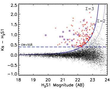
Figure 1.— Color-magnitude diagram for $H_{\mathrm{2}}S1$ detected objects. The blue solid/dotted line represents the limitation due to background noise at the $\Sigma=3$/$\Sigma=2$ level. The blue dashed line marks the excess cut corresponding to the rest-frame EW=50$\AA$. The red crosses are the 140 emission-line candidates. The blue squares mark the candidates with spec-$z$.

As shown in Figure 1, 146 emission-line candidates are selected with $\Sigma>3$ and EW $>50$ Å. To examine how many spurious sources will be selected by our criteria, we perform a “negative” selection with $K_{\rm s}-H_{\mathrm{2}}S1<-0.39$ mag and $-3\Sigma$ cut. Only one object being selected means our criteria enable a clean selection of emission-line object candidates. Furthermore, we perform a visual examination of our selected candidates. Of the 146, six are visually identified as spurious sources like spikes of bright stars or contaminations that were not rejected by data reduction. The other 140 candidates are expected to be objects with a strong emission line between Pa$\alpha$ at $z=0.14$ and Ly$\alpha$ at $z=16.52$. And 33 of the 140 objects are found to have spectroscopic redshifts from the catalog collected by Cardamone et al. (2010).

It is worth noting that the requirement of a secure detection ($>5\sigma$) in the $K_{\rm s}$ might miss emission-line objects with very high EWs. To quantify this effect, we re-examine $H_{2}S1$ sources and find 14 objects with $K_{\rm s}\geq$ 24.8 mag. Among them, six are visually identified as spurious sources. The other eight sources are very faint ($H_{2}S1>$22.5 mag), compared to the detection limit of $H_{2}S1=$ 22.8 mag. We suspect that their very high EWs ($>500$Å) would be dominated by noise and the intrinsic EWs could be lower. Considering that  emitters represent $30\%-40\%$ of all emitters (Hayes et al., 2010; Lee et al., 2012), less than three of the eight sources are expected to be  emitters. Moreover, they must be very low-mass galaxies with given $K_{\rm s}$ magnitudes. The missing fraction of  emitters with very high EWs is estimated to be very small ($<$ 5%). We therefore conclude that inclusion of the selection criterion $K_{\rm s}<$ 24.8 mag has negligible detrimental effects on our main results.

3.2. Photometric Redshifts and SED Modeling

To measure fluxes and construct SEDs for the selected 140 emission-line objects, we use 12 bands imaging data, including $U$, $B$, $V$, $R$ and $I$-band data from the Multiwavelength Survey by Yale-Chile (MUSYC; Gawiser et al., 2006), HST/ACS F606W ($V_{606}$) and F850LP ($z_{850}$) imaging from GEMS (Rix et al., 2004; Caldwell et al., 2008), HST/WFC3 F125W ($J_{125}$) and F160W ($H_{160}$) imaging from the Cosmic Assembly Near-infrared Deep Extragalactic Legacy Survey (CANDELS; Grogin et al., 2011; Koekemoer et al., 2011), and CFHT/WIRCam $J$ and $K_{\rm s}$ imaging (Hsieh et al., 2012) in combination with our $H_{2}S1$ data. Only 72 of the 140 have $J_{125}$ and $H_{160}$ data because CANDELS observations only cover the central part of ECDFS, i.e. the GOODS-South region. The 12 bands images have distinct PSFs. The HST images have PSFs with FWHM $\sim 0\farcs 1-0\farcs 16$, compared to $\sim 1\arcsec$ for the MUSYC images and $\sim 0\farcs 8$ for the CFHT images.

Instead of measuring fluxes within the same aperture from the 12 bands images downgraded to the worst PSF, we intend to maximize S/N for aperture-matched colors between the 12 bands. We first determine colors for MUSYC, HST and CFHT bands, respectively. Second, we match three sets of colors to establish SEDs from the $U$ to the $K_{\rm s}$. The aperture-matched fluxes in the $U$, $B$, $V$, $R$ and $I$ (and thus colors between them) are available for 124 of the 140 targets from the MUSYC public catalog (Cardamone et al., 2010). The other 16 are optically too faint to be detected by MUSYC observations. For the HST data set, $V_{606}$ and $z_{850}$ images are convolved with $H_{160}$ PSF, while $J_{125}$ and $H_{160}$ images are convolved with $z_{850}$ PSF. These operations enable us to match the four images to the same spatial resolution. An aperture of diameter of 1$\arcsec$ is used to measure fluxes from the convolved images and give aperture-matched colors between the four HST bands. Colors between CFHT $J$, $K_{\rm s}$ and $H_{2}S1$ bands are derived from photometry over the same area of a target using SExtractor in “dual-image” mode. The next step is to match MUSYC, HST and CFHT colors to the same aperture. This is done by deriving the aperture-matched color between the $J_{125}$ ($z_{850}$ instead if $J_{125}$ is not available) and $J$ bands, and that between the $V_{606}$ and $V$ bands. Since $J_{125}/z_{850}$-band PSF ($0\farcs 13$/$0\farcs 1$) is much smaller than $J$-band PSF ($0\farcs 8$), we convolve the $J_{125}/z_{850}$ image with the $J$-band PSF to match the spatial resolution of $J$-band image. An aperture of 2$\arcsec$ diameter is used to measure fluxes accordingly. Moreover, the MUSYC colors are linked to the HST-band colors by matching the interpolated $V_{606}$ between $V$- and $R$-band magnitudes with $V_{606}$. The aperture-matched colors establish the $U-K_{\rm s}$ SED. The SED is then scaled up to meet the total magnitude of $K_{\mathrm{s}}$ derived from aperture photometry within a diameter of 2$\arcsec$ corrected for missing flux out of the aperture (see Retzlaff et al. 2010 for more details). By doing so, we obtain SEDs for our 140 emission-line objects.

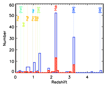
Figure 2.— Distribution of photo-$z$ for 138 selected emission-line candidates. The red shaded area shows the distribution of 33 candidates with spec-$z$. The dotted lines mark the emission-lines detected by the $H_{\mathrm{2}}S1$ filter at given redshifts.

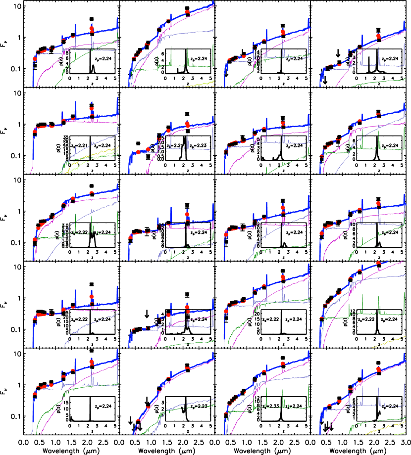
Figure 3.— Best-fit SEDs of  ELGs. The squares are the observed data points and circles are the best-fit data points from EAZY code (Brammer et al., 2008). The arrows show the upper limits of corresponding bands, which means the source is not detected or resolved in these bands. In each plan, the thick line shows the best-fit SED and light lines are the used templates; The inset plot shows the integrated probability of redshift.

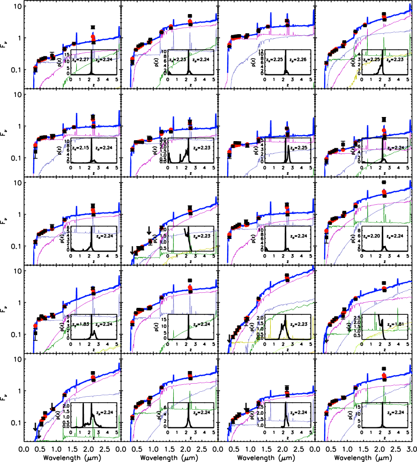
Figure 3.— (Continued).

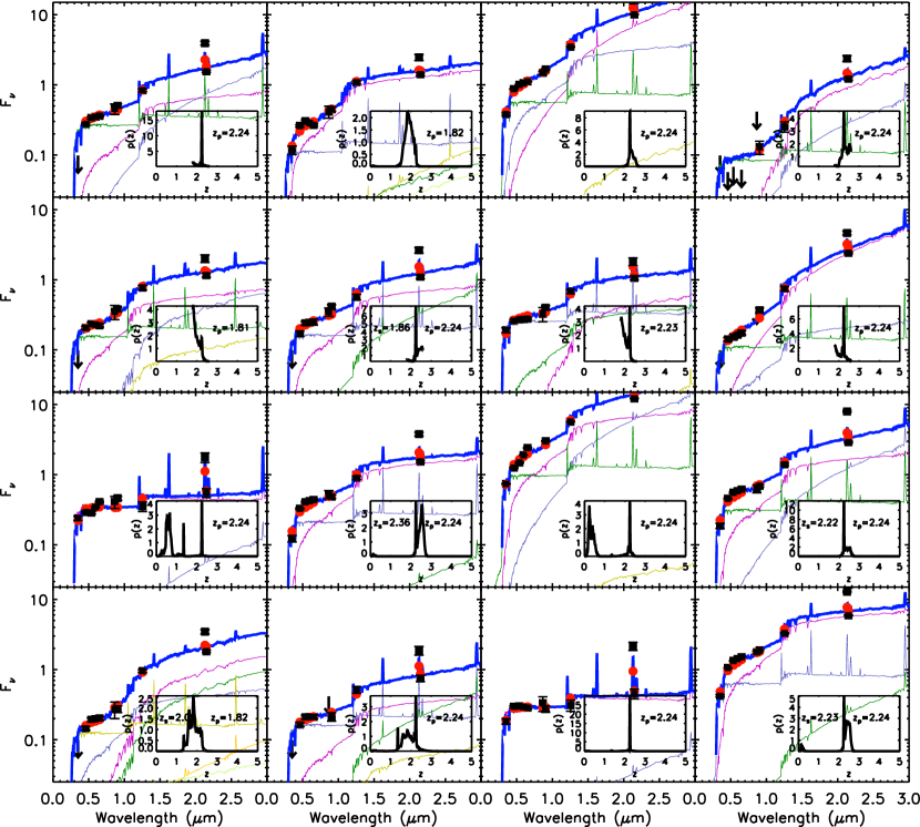
Figure 3.— (Continued).

The software tool EAZY (Easy and Accurate Redshifts from Yale; Brammer et al., 2008) is used to derive photometric redshifts (photo-$z$). The template-fitting method used in EAZY to estimate photo-$z$ suffers from the fact that template color frequently degenerates with redshift. The $K_{\mathrm{s}}$ magnitude is then taken as a Bayesian prior to assigning a low probability to a very low redshift and a similarly low probability for finding extremely bright galaxies at high-$z$. The emission-line objects selected with NIR narrow-band excess are mostly, if not all, SFGs (e.g., see Hayes et al., 2010). Therefore, the default library of galaxy templates in EAZY is chosen to derive photo-$z$. The library includes five templates generated based on the PÉGASE population synthesis models (Fioc & Rocca-Volmerange, 1997) and calibrated with synthetic photometry from semi-analytic models, and one template of young ($t=50$ Myr) and dusty ($A_{\mathrm{V}}=2.75$) starbursts. The combination of the six templates is able to model galaxies with colors over a broad range and minimize the color and redshift degeneracy. Moreover, the PÉGASE models provide a self-consistent treatment of emission lines. Among 140 emission-line objects, two have SED composed of $<5$ valid data points and fail to produce photo-$z$.

Figure 2 shows the distribution of photo-$z$ for the 138 objects. The 33 objects with spec-$z$ are shown by the hatched regions. The emission lines potentially detected by $H_{2}S1$ are marked. We can clearly see two prominent peaks at $z\sim 2.24$ and $z\sim 3.25$, corresponding to the emission lines  and [O III], respectively. These two peaks are confirmed by the spec-$z$ distribution. The good agreement between spec-$z$ and our photo-$z$ indicates that our $H_{2}S1$ data are critical to determining photo-$z$ to a relatively-high precision. Other two peaks at $z\sim 1.3$ and $z\sim 1.0$ contain 17 and 10 objects, respectively. The peak at $z\sim 1.3$ corresponds to [S III]$\lambda$9096, while the peak at $z\sim 1.0$ corresponds to P$\gamma\lambda$10935, P$\delta\lambda$10047 or He I$\lambda$10830 lines. The relatively high abundance of [S III]$\lambda$9096 was seldom reported in the literature. We further examine their properties in An et al. (2013). We note that two objects have photo-$z$ corresponding to no known strong emission lines. They are located close to the $\Sigma=3$ line in Figure 1. We argue that the two objects are likely noise contaminators.

Table 1 Multi-band Photometry of Our Sample of  ELGs

ID	Mag_$U$	Mag_$B$	Mag_$V$	Mag_$V_{\mathrm{606}}$	Mag_$R$	Mag_$I$	Mag_$z_{\mathrm{850}}$	Mag_$J_{\mathrm{125}}$	Mag_J	Mag_$H_{\mathrm{160}}$	Mag_$K_{\mathrm{s}}$	Mag_$H_{2}S1$	Mag_$24\mu$m
1	25.62$\pm$0.18	24.56$\pm$0.02	24.34$\pm$0.03	24.28$\pm$0.02	24.23$\pm$0.02	24.41$\pm$0.15	24.16$\pm$0.03	23.76$\pm$0.02	23.69$\pm$0.05	23.17$\pm$0.01	23.11$\pm$0.04	21.89$\pm$0.05	-99.99
2	-99.99	25.29$\pm$0.06	24.93$\pm$0.06	24.72$\pm$0.03	24.52$\pm$0.04	24.29$\pm$0.18	23.94$\pm$0.03	22.92$\pm$0.01	22.96$\pm$0.03	22.24$\pm$0.01	21.72$\pm$0.02	21.18$\pm$0.04	18.39 $\pm$0.21
3	-99.99	25.32$\pm$0.05	25.15$\pm$0.06	25.06$\pm$0.02	24.98$\pm$0.04	-99.99	24.68$\pm$0.03	24.22$\pm$0.02	24.09$\pm$0.06	23.73$\pm$0.02	23.28$\pm$0.04	22.43$\pm$0.07	-99.99
4	-99.99	-99.99	25.90$\pm$0.11	25.84$\pm$0.05	25.79$\pm$0.09	-99.99	25.40$\pm$0.07	24.85$\pm$0.04	24.65$\pm$0.11	24.16$\pm$0.02	23.65$\pm$0.07	22.84$\pm$0.12	-99.99
5	24.17$\pm$0.03	23.45$\pm$0.01	23.37$\pm$0.01	23.37$\pm$0.01	23.37$\pm$0.01	23.31$\pm$0.06	23.38$\pm$0.01	23.26$\pm$0.01	23.21$\pm$0.03	22.73$\pm$0.01	22.77$\pm$0.03	21.86$\pm$0.05	-99.99
6	…	…	…	25.19$\pm$0.03	…	…	26.25$\pm$0.17	24.62$\pm$0.03	24.51$\pm$0.10	23.90$\pm$0.02	24.20$\pm$0.12	22.80$\pm$0.12	-99.99
7	25.34$\pm$0.08	24.75$\pm$0.03	24.69$\pm$0.04	24.65$\pm$0.02	24.60$\pm$0.03	24.19$\pm$0.13	24.34$\pm$0.03	23.76$\pm$0.01	23.79$\pm$0.04	23.58$\pm$0.01	23.32$\pm$0.05	22.63$\pm$0.11	-99.99
8	26.34$\pm$0.18	25.39$\pm$0.05	25.14$\pm$0.05	25.09$\pm$0.02	25.04$\pm$0.05	24.96$\pm$0.24	24.55$\pm$0.03	23.86$\pm$0.01	23.80$\pm$0.04	23.45$\pm$0.01	22.89$\pm$0.03	22.53$\pm$0.09	-99.99
9	25.68$\pm$0.12	24.23$\pm$0.02	23.94$\pm$0.02	23.92$\pm$0.01	23.90$\pm$0.02	23.60$\pm$0.10	23.40$\pm$0.01	22.72$\pm$0.01	22.66$\pm$0.02	22.30$\pm$0.01	21.79$\pm$0.02	21.09$\pm$0.04	19.41 $\pm$0.32
10	25.55$\pm$0.08	24.83$\pm$0.03	24.74$\pm$0.03	24.78$\pm$0.02	24.82$\pm$0.04	24.75$\pm$0.19	24.71$\pm$0.03	24.53$\pm$0.02	24.38$\pm$0.08	24.10$\pm$0.02	24.14$\pm$0.11	22.74$\pm$0.11	-99.99
11	25.79$\pm$0.23	24.78$\pm$0.03	24.62$\pm$0.03	24.64$\pm$0.02	24.65$\pm$0.03	24.61$\pm$0.19	24.58$\pm$0.03	24.37$\pm$0.02	24.13$\pm$0.06	23.77$\pm$0.01	23.65$\pm$0.07	22.50$\pm$0.09	-99.99
12	25.45$\pm$0.09	24.50$\pm$0.02	24.31$\pm$0.03	24.33$\pm$0.01	24.34$\pm$0.02	24.33$\pm$0.15	24.21$\pm$0.02	23.70$\pm$0.01	23.56$\pm$0.04	23.40$\pm$0.01	23.06$\pm$0.04	22.41$\pm$0.08	-99.99
13	25.21$\pm$0.07	24.42$\pm$0.02	24.42$\pm$0.03	24.45$\pm$0.01	24.48$\pm$0.03	24.46$\pm$0.16	24.53$\pm$0.03	24.55$\pm$0.02	24.58$\pm$0.08	23.88$\pm$0.01	23.83$\pm$0.08	22.23$\pm$0.07	-99.99
14	-99.99	25.95$\pm$0.09	25.81$\pm$0.10	25.77$\pm$0.04	25.74$\pm$0.09	-99.99	25.67$\pm$0.08	25.21$\pm$0.04	25.06$\pm$0.13	24.37$\pm$0.02	24.80$\pm$0.18	22.99$\pm$0.13	-99.99
15	24.60$\pm$0.20	23.57$\pm$0.01	23.40$\pm$0.01	23.36$\pm$0.01	23.33$\pm$0.01	23.18$\pm$0.07	23.06$\pm$0.01	22.54$\pm$0.00	22.60$\pm$0.02	22.17$\pm$0.00	21.68$\pm$0.02	20.83$\pm$0.03	18.59 $\pm$0.23
16	25.05$\pm$0.08	23.96$\pm$0.02	23.64$\pm$0.02	23.46$\pm$0.01	23.28$\pm$0.01	22.88$\pm$0.05	22.68$\pm$0.01	21.91$\pm$0.00	21.88$\pm$0.01	21.29$\pm$0.00	20.73$\pm$0.01	19.81$\pm$0.01	17.82 $\pm$0.16
17	24.77$\pm$0.06	24.11$\pm$0.02	23.85$\pm$0.02	…	23.74$\pm$0.02	23.60$\pm$0.11	…	23.37$\pm$0.01	22.94$\pm$0.03	22.82$\pm$0.01	22.41$\pm$0.03	21.10$\pm$0.03	19.67 $\pm$0.35
18	-99.99	-99.99	-99.99	26.51$\pm$0.11	-99.99	-99.99	25.11$\pm$0.06	23.80$\pm$0.01	23.84$\pm$0.07	23.08$\pm$0.01	22.36$\pm$0.03	21.95$\pm$0.07	-99.99
19	25.86$\pm$0.15	24.85$\pm$0.04	24.64$\pm$0.04	24.50$\pm$0.02	24.36$\pm$0.03	24.06$\pm$0.15	23.85$\pm$0.03	23.02$\pm$0.01	22.91$\pm$0.03	22.49$\pm$0.01	21.94$\pm$0.02	21.24$\pm$0.04	19.05 $\pm$0.28
20	-99.99	-99.99	-99.99	25.45$\pm$0.04	-99.99	-99.99	24.72$\pm$0.04	23.83$\pm$0.01	24.18$\pm$0.07	23.21$\pm$0.01	22.73$\pm$0.03	21.89$\pm$0.05	19.71 $\pm$0.36
21	25.83$\pm$0.11	25.13$\pm$0.04	25.00$\pm$0.05	24.95$\pm$0.02	24.90$\pm$0.04	24.71$\pm$0.20	24.92$\pm$0.04	24.23$\pm$0.01	24.16$\pm$0.06	23.77$\pm$0.01	23.69$\pm$0.06	22.48$\pm$0.08	-99.99
22	25.11$\pm$0.15	24.12$\pm$0.02	23.85$\pm$0.02	23.77$\pm$0.01	23.69$\pm$0.02	23.55$\pm$0.09	23.31$\pm$0.01	22.76$\pm$0.00	22.72$\pm$0.03	22.40$\pm$0.00	22.13$\pm$0.02	21.46$\pm$0.05	-99.99
23	24.00$\pm$0.01	23.25$\pm$0.02	23.22$\pm$0.01	23.20$\pm$0.01	23.18$\pm$0.02	23.27$\pm$0.05	23.11$\pm$0.01	22.81$\pm$0.01	22.70$\pm$0.03	22.44$\pm$0.01	22.35$\pm$0.03	21.98$\pm$0.07	-99.99
24	25.10$\pm$0.07	24.44$\pm$0.02	24.24$\pm$0.03	24.15$\pm$0.01	24.06$\pm$0.03	23.78$\pm$0.10	23.46$\pm$0.02	22.64$\pm$0.01	22.63$\pm$0.03	22.14$\pm$0.00	21.69$\pm$0.02	21.25$\pm$0.04	-99.99
25	25.37$\pm$0.28	24.41$\pm$0.02	24.27$\pm$0.02	24.25$\pm$0.01	24.22$\pm$0.02	24.18$\pm$0.13	24.12$\pm$0.02	23.74$\pm$0.01	23.78$\pm$0.08	23.44$\pm$0.01	23.41$\pm$0.07	22.64$\pm$0.12	-99.99
26	25.09$\pm$0.06	24.48$\pm$0.02	24.47$\pm$0.03	24.47$\pm$0.01	24.48$\pm$0.03	24.20$\pm$0.13	24.19$\pm$0.02	23.66$\pm$0.01	23.69$\pm$0.04	23.65$\pm$0.01	23.38$\pm$0.05	22.91$\pm$0.12	-99.99
27	24.57$\pm$0.05	23.81$\pm$0.02	23.56$\pm$0.01	23.57$\pm$0.01	23.58$\pm$0.02	-99.99	23.75$\pm$0.04	…	23.37$\pm$0.04	…	22.90$\pm$0.04	22.41$\pm$0.01	-99.99
28	26.23$\pm$0.14	25.55$\pm$0.05	25.47$\pm$0.07	25.39$\pm$0.05	25.32$\pm$0.06	24.90$\pm$0.22	…	…	24.85$\pm$0.14	…	24.33$\pm$0.14	22.92$\pm$0.13	-99.99
29	25.56$\pm$0.10	24.96$\pm$0.04	24.86$\pm$0.04	24.77$\pm$0.03	24.67$\pm$0.03	24.38$\pm$0.16	…	…	23.80$\pm$0.06	…	23.41$\pm$0.07	22.71$\pm$0.12	-99.99
30	-99.99	26.68$\pm$0.15	26.30$\pm$0.14	26.29$\pm$0.10	26.27$\pm$0.14	-99.99	25.79$\pm$0.21	…	24.66$\pm$0.11	…	23.55$\pm$0.06	23.09$\pm$0.14	-99.99
31	25.26$\pm$0.07	24.53$\pm$0.02	24.45$\pm$0.03	24.35$\pm$0.02	24.26$\pm$0.02	24.03$\pm$0.11	24.21$\pm$0.05	…	23.77$\pm$0.05	…	23.48$\pm$0.06	22.69$\pm$0.10	-99.99
32	25.32$\pm$0.37	24.19$\pm$0.02	23.90$\pm$0.02	23.85$\pm$0.02	23.80$\pm$0.02	23.64$\pm$0.11	23.38$\pm$0.04	…	22.88$\pm$0.04	…	22.05$\pm$0.03	20.98$\pm$0.04	18.76 $\pm$0.25
33	25.15$\pm$0.23	24.04$\pm$0.03	23.82$\pm$0.02	23.91$\pm$0.02	24.00$\pm$0.05	23.69$\pm$0.07	23.85$\pm$0.05	…	23.06$\pm$0.04	…	22.04$\pm$0.02	21.62$\pm$0.05	-99.99
34	25.34$\pm$0.08	24.44$\pm$0.02	24.18$\pm$0.02	24.19$\pm$0.02	24.19$\pm$0.02	24.06$\pm$0.12	24.01$\pm$0.05	…	23.24$\pm$0.03	…	22.76$\pm$0.03	21.88$\pm$0.04	-99.99
35	-99.99	26.45$\pm$0.18	26.15$\pm$0.18	25.91$\pm$0.10	25.68$\pm$0.11	25.18$\pm$0.39	25.03$\pm$0.14	…	23.42$\pm$0.05	…	21.99$\pm$0.02	21.59$\pm$0.05	19.34 $\pm$0.31
36	-99.99	25.54$\pm$0.06	25.26$\pm$0.06	25.13$\pm$0.07	25.00$\pm$0.04	24.83$\pm$0.22	24.31$\pm$0.11	…	23.50$\pm$0.04	…	22.82$\pm$0.04	22.23$\pm$0.07	-99.99
37	-99.99	-99.99	26.51$\pm$0.18	26.08$\pm$0.09	25.65$\pm$0.08	-99.99	25.34$\pm$0.14	…	24.25$\pm$0.08	…	23.07$\pm$0.04	22.50$\pm$0.08	-99.99
38	25.59$\pm$0.12	24.71$\pm$0.04	24.47$\pm$0.04	24.39$\pm$0.03	24.32$\pm$0.03	24.39$\pm$0.20	23.98$\pm$0.06	…	23.19$\pm$0.04	…	22.47$\pm$0.04	22.03$\pm$0.08	19.48 $\pm$0.33
39	-99.99	25.11$\pm$0.06	24.84$\pm$0.05	24.70$\pm$0.03	24.56$\pm$0.06	-99.99	24.21$\pm$0.06	…	23.70$\pm$0.06	…	23.06$\pm$0.05	22.49$\pm$0.09	-99.99
40	25.44$\pm$0.12	24.70$\pm$0.04	24.48$\pm$0.04	24.43$\pm$0.03	24.38$\pm$0.03	24.15$\pm$0.17	24.15$\pm$0.07	…	23.40$\pm$0.05	…	22.74$\pm$0.04	21.87$\pm$0.07	-99.99
41	-99.99	24.92$\pm$0.03	24.70$\pm$0.04	24.66$\pm$0.02	24.62$\pm$0.03	24.37$\pm$0.15	24.27$\pm$0.06	…	23.72$\pm$0.04	…	23.04$\pm$0.04	22.03$\pm$0.06	-99.99
42	26.11$\pm$0.16	25.26$\pm$0.05	25.09$\pm$0.05	25.16$\pm$0.04	25.22$\pm$0.05	24.75$\pm$0.22	24.66$\pm$0.08	…	23.70$\pm$0.06	…	23.42$\pm$0.06	22.81$\pm$0.12	-99.99
43	24.70$\pm$0.06	23.80$\pm$0.02	23.65$\pm$0.02	23.59$\pm$0.01	23.53$\pm$0.02	23.22$\pm$0.08	23.10$\pm$0.03	…	22.30$\pm$0.02	…	21.14$\pm$0.01	20.67$\pm$0.02	17.73 $\pm$0.16
44	-99.99	-99.99	-99.99	-99.99	-99.99	-99.99	25.87$\pm$0.21	…	25.14$\pm$0.17	…	23.43$\pm$0.05	22.71$\pm$0.10	-99.99
45	-99.99	25.16$\pm$0.05	25.03$\pm$0.05	25.05$\pm$0.04	25.07$\pm$0.05	24.59$\pm$0.19	24.50$\pm$0.07	…	23.73$\pm$0.06	…	23.29$\pm$0.06	22.69$\pm$0.11	-99.99
46	-99.99	25.26$\pm$0.07	24.89$\pm$0.05	24.87$\pm$0.03	24.84$\pm$0.07	24.48$\pm$0.11	24.30$\pm$0.05	…	23.95$\pm$0.07	…	23.23$\pm$0.05	22.29$\pm$0.07	-99.99
47	25.25$\pm$0.07	24.92$\pm$0.03	24.87$\pm$0.04	24.86$\pm$0.03	24.85$\pm$0.04	24.67$\pm$0.19	24.45$\pm$0.07	…	23.87$\pm$0.06	…	23.39$\pm$0.06	22.81$\pm$0.11	-99.99
48	-99.99	25.86$\pm$0.07	25.77$\pm$0.09	25.69$\pm$0.06	25.62$\pm$0.08	-99.99	24.82$\pm$0.09	…	24.05$\pm$0.08	…	22.77$\pm$0.04	22.07$\pm$0.07	-99.99
49	24.99$\pm$0.06	24.77$\pm$0.03	24.79$\pm$0.04	24.60$\pm$0.02	24.41$\pm$0.03	24.41$\pm$0.16	24.27$\pm$0.06	…	24.57$\pm$0.13	…	24.08$\pm$0.12	22.82$\pm$0.13	-99.99
50	25.57$\pm$0.08	24.51$\pm$0.02	24.27$\pm$0.02	24.23$\pm$0.02	24.20$\pm$0.02	24.00$\pm$0.10	24.08$\pm$0.04	…	23.41$\pm$0.04	…	22.82$\pm$0.03	21.85$\pm$0.05	-99.99
51	25.04$\pm$0.06	24.46$\pm$0.09	24.28$\pm$0.07	24.01$\pm$0.02	23.76$\pm$0.07	-99.99	23.52$\pm$0.04	…	22.82$\pm$0.03	…	21.99$\pm$0.02	21.28$\pm$0.04	-99.99
52	25.36$\pm$0.11	24.39$\pm$0.03	24.18$\pm$0.03	24.12$\pm$0.02	24.07$\pm$0.03	24.04$\pm$0.15	23.94$\pm$0.05	…	23.17$\pm$0.06	…	22.38$\pm$0.04	21.29$\pm$0.04	20.18 $\pm$0.44
53	-99.99	25.90$\pm$0.07	25.59$\pm$0.07	25.56$\pm$0.05	25.54$\pm$0.07	25.21$\pm$0.29	25.21$\pm$0.13	…	23.85$\pm$0.06	…	23.15$\pm$0.05	22.45$\pm$0.08	-99.99
54	-99.99	25.58$\pm$0.07	25.32$\pm$0.06	25.32$\pm$0.04	25.31$\pm$0.06	-99.99	25.30$\pm$0.14	…	24.34$\pm$0.11	…	23.93$\pm$0.10	22.94$\pm$0.14	-99.99
55	25.42$\pm$0.09	24.89$\pm$0.03	24.88$\pm$0.04	24.91$\pm$0.03	24.93$\pm$0.04	24.77$\pm$0.22	24.97$\pm$0.10	…	24.84$\pm$0.17	…	24.43$\pm$0.15	22.74$\pm$0.13	-99.99
56	24.48$\pm$0.05	23.48$\pm$0.01	23.23$\pm$0.01	23.16$\pm$0.01	23.10$\pm$0.01	22.92$\pm$0.06	22.85$\pm$0.01	…	22.25$\pm$0.03	…	21.61$\pm$0.02	20.77$\pm$0.03	-99.99

^aSources are not detected. ^bSources could not be resolved in MUSYC observation. ^cSources are not covered by CANDELS or GEMS observation. ^∗Three X-ray sources.

Accounting for potential uncertainties in photo-$z$ (see also Lee et al., 2012), we take 56 objects with $1.8<z_{\mathrm{phot}}<2.6$ as  emitters at $z=2.24$. Similarly, we identify 34 [O III] emitters at $z=3.25$, two [O II] emitters at $z=6.72$, and other emitters at lower redshifts, including Pa$\alpha$ at $z=0.14$, [Fe II] at $z=0.30$ and [S III] at $z=1.23/1.35$. Here the percentage of  emitters among all emitters is 40% (56/140), consistent with $\sim$36% in Hayes et al. (2010) and Lee et al. (2012). We show the best-fit SED models and the probability function of photo-$z$ for the 56  emitters in Figure 3. Table 1 lists their multi-band photometry and Table 2 gives their photo-$z$ and spec-$z$.

4. PROPERTIES OF  EMISSION-LINE GALAXIES

4.1. X-Ray Properties

We first match our  emitters with the X-ray source catalog of 4 Ms Chandra exposure in CDFS (Xue et al., 2011) to examine their X-ray properties. Three out of 56  emitters are detected in X-ray (X-ray source ID = 29, 399, and 435 in the Chandra catalog), with absorption-corrected rest-frame 0.5-8 keV luminosities $2.60\times 10^{43},2.76\times 10^{42}$, and $1.15\times 10^{43}$ erg s^-1, respectively. While the faintest X-ray among the three (X-ray source ID = 399) was identified as a galaxy, the other two more luminous X-ray sources were classified as active galactic nuclei (AGNs), both of which are likely obscured AGNs according to their X-ray hardness ratios (Xue et al., 2011). In addition, we find that the three  sources have luminosity $L_{\mathrm{H\alpha}}>10^{43.5}$ erg s^-1, being the most luminous ones in our sample and also the most massive ones with $M>10^{11}\,M_{\odot}$ (see Section 4.5).

For the other non-detected X-ray  emitters, we perform X-ray stacking analyses using 4 Ms Chandra exposures. We exclude sources with no X-ray coverage or with contaminations from nearby bright X-ray sources. We finally stacked X-ray images of 42  emitters, yielding an effective exposure time of 106 Ms. We find a marginal detection in the stacked 0.5-2 keV image (S/N = 2.5), and obtain an average rest frame 0.5-2.0 keV X-ray luminosity of $3.5\pm 1.4\times 10^{42}$ erg s^-1 by assuming a power-law spectrum with photon index of 2.0. This confirms that the vast majority of our sample consists of star-forming ones.

4.2. Morphologies

HST/ACS $V_{606}$ and $z_{850}$ imaging data are used to examine morphologies. The two bands correspond to the rest-frame 1839Å and 2794Å for $z=2.24$. HST/WFC3 imaging data from CANDELS are available for 26 of our 56 sample targets.

Table 2 Physical Parameters of Our Sample of  ELGs

ID	Photo-$z$	Spec-$z$	A(H$\alpha$) (mag)	log H$\alpha$ (erg s-1)	log $(M/M_{\odot})$	Morphology
1	2.25	…	1.07	42.99	9.95	1
2	2.24	…	1.92	43.39	10.75	2
3	2.24	…	1.70	42.94	9.42	4
4	2.24	…	2.00	42.87	9.54	5
5	2.25	2.21	0.65	42.76	9.33	2
6	2.24	2.22	0.00	42.22	9.81	1
7	2.24	…	0.36	42.25	9.81	1
8	2.24	…	1.40	42.52	10.15	2
9	2.25	2.23	1.06	43.17	10.62	3
10	2.25	…	0.67	42.52	9.21	4
11	2.25	…	1.41	42.86	9.61	2
12	2.25	…	0.64	42.46	9.91	2
13	2.25	2.22	0.00	42.46	9.35	2
14	2.24	…	0.00	42.19	9.14	3
15	2.24	2.23	1.67	43.55	10.69	2
16	2.24	2.22	1.73	44.00	11.36	2
17	2.24	…	1.58	43.47	10.35	3
18	2.24	…	2.10	42.99	10.53	5
19	2.24	2.34	1.70	43.30	10.74	3
20	2.24	…	2.10	43.31	10.57	3
21	2.24	2.28	0.95	42.70	9.76	4
22	2.24	2.23	0.53	42.70	10.23	3
23	2.26	2.26	0.03	42.28	10.14	2
24	2.24	2.25	1.62	43.14	10.93	3
25	2.25	2.15	0.04	42.17	9.50	4
26	2.23	…	0.04	41.91	9.36	4
27	2.26	…	0.16	42.17	9.98	1
28	2.25	…	0.93	42.55	9.45	4
29	2.24	…	0.05	42.12	9.87	3
30	2.24	…	1.83	42.53	9.82	5
31	2.25	…	0.01	42.13	9.39	1
32	2.25	2.21	1.32	43.43	10.49	2
33	2.24	1.83	1.81	43.11	10.53	1
34	2.24	…	0.36	42.63	10.21	1
35	2.24	…	1.93	43.14	10.91	5
36	1.82	…	1.33	42.77	9.94	4
37	2.24	…	1.87	42.86	10.17	5
38	2.24	…	1.05	42.58	10.38	3
39	2.25	…	0.18	42.19	9.89	5
40	2.24	…	1.14	42.75	10.22	2
41	2.24	…	1.40	43.01	9.86	4
42	1.83	…	0.18	42.08	9.51	2
43	2.25	…	1.77	43.50	11.14	4
44	2.25	…	1.06	42.52	10.23	5
45	1.82	…	0.00	42.06	9.86	3
46	2.24	1.87	1.08	42.77	9.77	3
47	2.24	…	0.09	42.03	9.83	3
48	2.24	…	2.09	43.18	10.58	3
49	2.24	…	0.54	42.41	8.40	1
50	2.25	2.36	0.12	42.57	10.02	1
51	2.24	…	1.44	43.10	10.71	1
52	2.25	2.22	1.32	43.28	10.52	2
53	1.83	2.10	0.14	42.24	9.91	5
54	2.24	…	1.05	42.50	9.46	4
55	2.24	…	0.42	42.45	9.26	1
56	2.25	2.23	0.23	43.02	10.64	2

^a1:Two components; 2:merger; 3: spiral/diffuse/clumpy; 4:compact; 5:UV-faint. ^∗Three X-ray sources (corresponded ID = 435, 29 and 399 in the Chandra catalog).

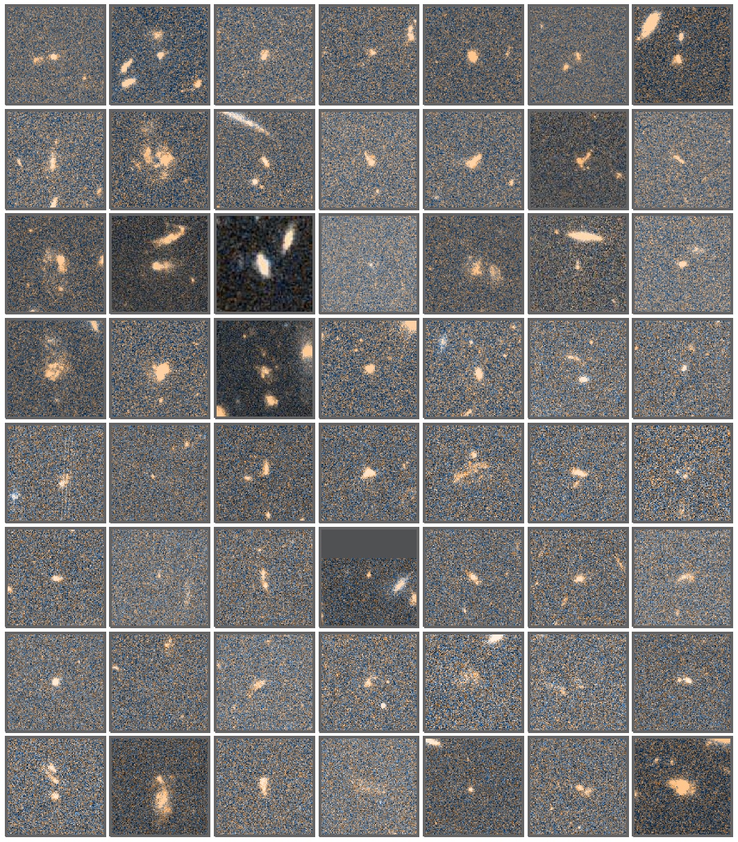
Figure 6.— The $6\arcsec\times 6\arcsec$ HST color images are made of ACS $V_{606}$ and $z_{850}$ from GEMS and GOODS. The 56  ELGs listed in Table 1 are given from left to right and top to bottom. One image (the 3rd from the top and 3rd from the left) is made of HST/WFC3 $J_{125}$ and $H_{160}$ from CANDELS due to no $V_{606}$ observation.

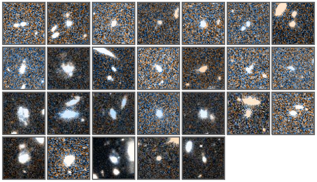
Figure 7.— HST/WFC3 color images of the first 26  ELGs given in Table 1. The color images are made of $J_{125}$ and $H_{160}$ from CANDELS. Each thumbnail image has a size of $6\arcsec\times 6\arcsec$ corresponding to 49 kpc$\times$49 kpc at $z=2.24$.

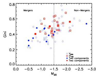
Figure 8.— Gini vs. $M_{\mathrm{20}}$ coefficients for our sample of 56  ELGs. The circles represent the results derived from the HST F606W imaging data. The squares are the results from HST F160W imaging data for the 26  ELGs in GOODS-South. The solid circles and solid squares are the sample galaxies with two major components. The vertical line at $M_{\mathrm{20}}\sim-1.5$ is the empirical delineation between mergers and non-mergers (Stott et al., 2013).

Figure 6 shows HST $V_{606}$+$z_{850}$ color image stamps for 55  ELGs and $J_{125}$+$H_{160}$ color image stamp for one (the third from the top and third from the left). One can see that the  ELGs in our sample show a variety of morphologies. The 56  ELGs are visually classified by three of us (X. Z. Z, F. X. A and G. W. F) and the median types are given in Table 2. About 20% (11/56) of the sample galaxies contain two major components of similar color and are separated by $\sim 1\arcsec-2\arcsec$ ($8-17$ kpc), which eliminates the possibility of them being multiple clumps within a single galaxy; 25% (14/56) appear to be merger remnants with tails, ‘tadpole’, or a peculiar shape; 23% (13/56) show spiral/diffuse/clumpy morphologies; 18% (10/56) are compact; 14% (8/56) are too faint to be resolved ($V_{606}<26$). We point out that the $V_{606}/z_{850}$-faint  galaxies are indeed dusty starbursts and their rest-frame UV lights are heavily attenuated. The UV-selection (e.g., Lyman break technique) is unable to pick up such dusty SFGs. This also suggests that the dust extinction of SFGs varies in a wide range. Of three X-ray sources, two are found in merging systems and one is a compact galaxy.

We notice that roughly 10% (6/56) of  ELGs exhibit an apparent offset ($>0\farcs 5$) between the central position in optical and NIR, indicating the complexity of morphologies in the rest-frame UV due to star formation activity and dust attenuation. Figure 7 shows HST $J_{125}$+$H_{160}$ color image stamps for the first 26 of the 56  ELGs. Still, our morphological classifications from $V_{606}$/$z_{850}$ images are mostly consistent with those from $J_{125}$/$H_{160}$ images for the 26  ELGs in GOODS-South. The similarity in morphology between the rest-frame UV and the rest-frame optical for high-$z$ SFGs are also claimed by other studies (e.g., Papovich et al., 2005; Law et al., 2012).

We also measure the morphological parameters Gini (the relative distribution of the galaxy pixel flux values) and $M_{\mathrm{20}}$ (the second-order moment of the brightest 20% of the galaxy’s flux coefficients; Lotz et al., 2004) to quantify galaxy morphologies (Fang et al., 2012). Figure 8 shows the results. About half of our sample has $M_{\mathrm{20}}>\sim-1.5$, satisfying the empirical cut for mergers (Stott et al., 2013). This is consistent with our result base on visual classification.

4.3. Dust Extinction

We estimate dust extinction from SEDs. Generally speaking, dust extinction mostly effects the young stellar population of a galaxy because new stars are formed in dusty environments. On the other hand, the young population can be divided into two components: unattenuated and attenuated. As described in Section 3.2, we made use of EAZY code to fit SEDs with models from combination of six representative galaxy templates. One in the six templates represents a young and dusty starburst with $A_{\mathrm{V}}=2.75$ mag. The other five templates represent distinct stellar populations without dust attenuation. Thus, the best-fit models to a galaxy SED implying not only the best photo-$z$, but also the percentage of each template in total (Brammer et al., 2008). Therefore, the young and dusty starburst template can be used to approximately trace the amount of dust attenuation in a galaxy. The total effective extinction $A_{\mathrm{V}}$ to the entire galaxy relies on the fraction of the dusty starburst component in the SED. Accordingly, we calculated $A_{\mathrm{V}}$ using the best-fit models composed of six templates given by EAZY. Figure 3 shows the decomposition of the best-fit models into the six components. Here the $A_{\mathrm{V}}$ is limited to $A_{\mathrm{V}}\leq 2.75$ mag adopted by the dusty starburst template, although some -selected SFGs may be very dusty with $A({\rm H\alpha})$ equal to several magnitudes (e.g., Garn et al., 2010; Sobral et al., 2012). We point out that this limitation is not crucial to our results and our main conclusions are not affected. We come back to this point in Section 5.

In addition, 12 of the 56  ELGs are found to have 24 $\mu$m counterparts. The 24 $\mu$m catalog is extracted from deep Spitzer 24 $\mu$m imaging of the Far-Infrared Deep Extragalactic Legacy survey (Dickinson & FIDEL Team, 2007) using the PSF-fitting method of Zheng et al. (2006). The 3 $\sigma$ detection limit is 24.6 $\mu$ Jy, corresponding to the 50% completeness limit. The cross correlation between the two catalogs is done with a matching radius of 1$\farcs$2. We list their 24 $\mu$m magnitudes in Table 1. We find that all the 12 objects have extinction $>$ 1 mag and SFRs $>$ 20 $M_{\odot}\,{\rm yr}^{-1}$ (see Section 4.4). The 12 sample targets are indeed dusty starburst galaxies. This confirms that our method works well in estimating dust extinction.

4.4.  Luminosities and SFRs

Following Ly et al. (2011), we derive  + [N II] flux from the narrow-band excess $K_{\mathrm{s}}-H_{2}S1$ and $K_{\mathrm{s}}$ total magnitude using the formula

$${F_{L}=\Delta{\rm NB}\frac{f_{\rm NB}-f_{K_{\rm s}}}{1-(\Delta{\rm NB}/\Delta K_{\rm s})}},$$ (2)

where $f_{\rm NB}$ and $f_{K_{\rm s}}$ are fluxes given in the units of erg s^-1 cm^-2 Å^-1 for the $H_{2}S1$- and $K_{\rm s}$-band with filter width $\Delta{\rm NB}=293$ Å and $\Delta K_{\rm s}=3250$ Å, respectively.

We use [N II]/ = 0.117 to correct the contribution of [N II] $\lambda\lambda$6548,6583 and obtain the observed  fluxes (Hayes et al., 2010). The selection cut EW $>50$ Å together with the 5$\sigma$ depths of $H_{2}S1=22.8$ and $K_{\rm s}=24.8$ determines an  flux detection limit $>2.1\times 10^{-17}$ erg s^-1 cm^-1 Hz^-1. Differing from low-$z$ SFGs, the high-$z$ ones seem to show little difference between extinction derived from continuum and nebular lines (Erb et al., 2006b). We employ the Calzetti extinction law to estimate attenuation to  line $A({\rm H\alpha})$ from $A_{\mathrm{V}}$ which is derived from the SED modeling (Calzetti et al., 2000). The intrinsic  fluxes are estimated from the observed  fluxes with correction for extinction $A({\rm H\alpha})$. Then  luminosity is calculated with $z=2.24$.

The  luminosity is an estimator of SFR. We follow Kennicutt & Evans (2012, hereafter K12) to calculate SFR using

$$\log({\rm SFR}/M_{\odot}\,{\rm yr}^{-1})=\log L_{\mathrm{H\alpha}}-41.27,$$ (3)

where $L_{\mathrm{H\alpha}}$ is the extinction-corrected  luminosity in the units of erg s^-1. The SFR is calibrated with STARBURST99 model (Leitherer et al., 1999) and Kroupa IMF, differing from that given in Kennicutt (1998, hereafter K98). Table 2 in Kennicutt & Evans (2012) gives the conversion between K12 and K98 calibrations. For , SFR${}_{\mathrm{K12}}/$SFR${}_{\mathrm{K98}}=0.68$.

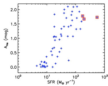
Figure 9.— Relationship between SFR and SED-derived extinction for our sample of 56  ELGs at $z$ = 2.24. The red squares mark three X-ray sources.

Figure 9 shows the estimated SFR versus  extinction. The data points spread mainly from 3 to 300 $M_{\odot}\,{\rm yr}^{-1}$ in SFR and from 0 to 2.2 mag in  extinction $A({\rm H\alpha})$. A correlation between SFR and H$\alpha$ extinction is apparent. The increase of extinction at an increasing SFR found for  ELGs is also seen for low-$z$ SFGs (e.g., Garn & Best, 2010) and high-$z$ SFGs (Ly et al., 2012; Sobral et al., 2012; Domínguez et al., 2013; Kashino et al., 2013).

4.5. Stellar Masses

The software FAST (Fitting and Assessment of Synthetic Templates; Kriek et al., 2009) is used to estimate stellar mass for our sample. The stellar population synthesis (SPS) models from Maraston (2005) and a Kroupa IMF (Kroupa, 2001) are adopted. We fit the SPS models with exponentially declining star formation histories and the star formation timescale $\tau$ from 10 Myr to 10 Gyr in steps of 0.5 dex. The metallicity is fixed to solar ($Z$ = 0.02) and the dust extinction is modeled by the Calzetti reddening law, with $A_{v}$ from 0 to 3 mag in steps of 0.01 mag. The ages of the model stellar populations range from 0.1 Myr to the age of the universe. The best photo-$z$ from EAZY is taken as input to FAST (see Kriek et al. 2009 for more details). Figure 10 shows the distribution of our sample galaxies in stellar mass and SFR. Three X-ray sources are marked with red squares. The vast majority of the sample galaxies have a stellar mass $9<\log(M/M_{\odot})<11$. The object has the lowest stellar mass $\log(M/M_{\odot})=8.40$ is faint in the $K_{\mathrm{s}}$-band but with a high EW and very blue color. From Figure 10, we can see that the  ELGs exhibit a correlation between stellar mass and SFR, which is known as the main sequence of SFGs (e.g., Elbaz et al., 2007; Daddi et al., 2007; Wuyts et al., 2011b). The dashed line describes the best fit to the mass-SFR correlation (three X-ray sources are removed), having a slope of 0.81. The scatter of this relation is 0.35 dex.

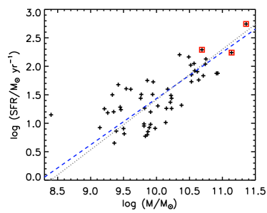
Figure 10.— The Mass-SFR relation of our 56  ELGs. The three red squares are X-ray-detected AGNs. The blue dashed line is a linear fit to the mass-SFR relation, giving a best-fit slope of 0.81. The gray dotted line is the fit without the lowest stellar mass one, giving a best-fit slope of 0.88. The three X-ray sources are removed in both fittings.

5. THE  LF AT $z=2.24$

One of our goals is to revisit the  LF and examine the influence of extinction correction. First, we commit Monte Carlo simulation to quantify the incompleteness of sample selection. After that, we determine the function of intrinsic  luminosities at $z=2.24$ using our sample of 53 X-ray-undetected  galaxies. Finally, we show that a constant extinction correction to the observed  luminosities results in an  LF similar to the results in previous works.

5.1. Completeness

A Monte Carlo simulation is used to derive the detection completeness as a function of intrinsic  luminosity. We assume that the intrinsic  LF is described by a Schechter function with $L_{\mathrm{H\alpha}}^{*}=10^{42.88}$, $\alpha=-1.60$ and $\log\phi^{*}=-1.79$ from Sobral et al. (2013). The $H_{2}S1$ filter centered at $\lambda_{\mathrm{c}}=2.130\,\micron$ has a width of $\Delta\lambda=0.0293$ $\micron$, corresponding to $2.225<z<2.267$ for . We use the averaged volume, corresponding to this redshift bin , as our effective volume. The brighter ELGs are detectable over a wider range of the filter transmission than the faint one. Therefore, we adopt a wider redshift span of $2.2<z<2.29$ to account for the entire wavelength coverage of the filter curve in our simulation. Then we can estimate the contamination rate of bright ELGs from low-$z$ (2.200 $<z<$ 2.225) and high-$z$ (2.267 $<z<$ 2.290). We generated a mock catalog of 30 million galaxies with  emission lines satisfying the given LF and the given redshift range. In practice, the simulated galaxies are divided into 30 redshift bins. In each redshift bin, the galaxies are divided again into 500 bins between $40<\log(L_{\mathrm{H\alpha}}/{\rm erg\,s^{-1}})<50$. Each bin contains on average 2000 galaxies. The contribution of [N II] is added to the simulated  using [N II]/ = 0.117. Dust attenuation is applied following the relation given in Figure 9 with a scatter of 0.38 in $A({\rm H\alpha})$ taken into account. Furthermore, a Gaussian line profile with $\sigma=200$ km s^-1 is adopted to convolve  at given redshifts with the $H_{2}S1$ filter transmission curve to simulate the observed +[N II] fluxes.

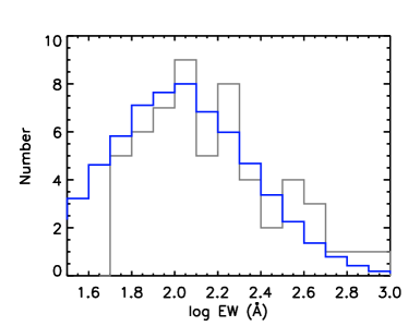
Figure 11.— Comparison of the modeled and observed EW distributions. The blue thick line shows the best matched model with mean $\log($EW${}_{\rm rest})$ = 2.00 and $\sigma\,[\log($EW$\mathrm{rest}/$Å)] = 0.35 and is scaled to match the observed distribution (gray line).

To link  + [N II] of a given flux to $H_{2}S1$ and $K_{\mathrm{s}}$ magnitudes of a galaxy, one needs to know the EW of the line. The intrinsic distribution of EW of  + [N II] is fairly similar to the observed distribution of rest-frame EW (Lee et al., 2007). We assume a log-normal distribution of EW for  + [N II] following Ly et al. (2011). Since the observed EWs of our sample are affected by noise as shown in Figure 1, we take the noise effects into account and infer the best-matched distribution as follows. A set of log-normal EW distributions are generated with the mean $\log($EW${}_{\rm rest})$ spanning between 1.8 and 2.3 and the spread $\sigma\,[\log($EW_rest/Å)] between 0.15 and 0.65. A step of 0.1 dex is adopted for the two parameters. Assuming that the flux of  + [N II] is not correlated with its EW, we randomly assign EWs satisfying a modeled EW distribution to the observed  + [N II] fluxes and give $H_{2}S1$ and $K_{\mathrm{s}}$ magnitudes. Added to the photon noise and sky background noise from our $H_{2}S1$ and $K_{\mathrm{s}}$ images (see also Ly et al., 2012), the simulated galaxies can be selected by $H_{2}S1-K_{\mathrm{s}}$ selection criteria as shown in Figure 1. By doing so, we model the ‘observed’ EW distribution for each of input intrinsic EW distributions under the same conditions as our $H_{2}S1$ and $K_{\rm s}$ observations. Comparing the modeled EW distributions with the observed EW distribution of our sample and minimizing the $\chi^{2}$, we obtain the intrinsic EW distribution best matching the observed EW distribution. The model with mean $\log($EW${}_{\rm rest})$ = 2.00 and $\sigma\,[\log($EW${}_{\rm rest}/$Å)] = 0.35 best reproduces the observed distribution of our sample galaxies. We show the best-matched mode in comparison with the observed distribution in Figure 11. This distribution is taken to randomly assign EWs to the mock catalog of simulated  + [N II] galaxies, thus making it possible to obtain $H_{2}S1$ and $K_{\mathrm{s}}$ magnitudes.

Accounting for the photon noise and sky noises from our $H_{2}S1$ and $K_{\rm s}$ images, the simulated  ELGs are selected using the criteria as shown in Figure 1. By doing so, we obtained the fraction of the mock galaxies picked up by our selection at given intrinsic  fluxes, giving the completeness as a function of the intrinsic  luminosity shown in Figure 12. Because the completeness curve is insensitive to the input Schechter function in the simulation, we employ the completeness curve given in Figure 12 to determine  LF using our sample. Note that the volume correction and completeness estimate for our sample root on the redshift bin $2.225<z<2.267$ and the final completeness curve accounts for all major effects involved in our observation and selection.

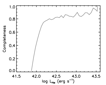
Figure 12.— Completeness as a function of  luminosity.

5.2. Determination of  LF

We determine the  LF at $z=2.24$ using our sample of 53  ELGs. Three X-ray sources are excluded to avoid AGN contamination. A volume of $5.40\times 10^{4}$ Mpc³ is calculated from the coverage of 383 arcmin² of our sample and a redshift span $2.225<z<2.267$. By dividing our sample into five bins in $\log(L_{\rm H\alpha})$ from 42.0 to 43.5 and taking the completeness correction, we obtained our  LF data points as shown in Figure 13. The error bars represent mainly the Poisson noise. We fit the data points with a Schechter function (Schechter, 1976) in the form of

$$\begin{split}&\Phi(\log L)\,d(\log L)=\\ &\ln(10)\,\Phi^{\star}\,10^{(\alpha+1)(\log L-\log L^{\star})}\,\exp[-10^{\log L-\log L^{\star}}]\,d(\log L),\end{split}$$ (4)

where $L^{\star}$ is the characteristic luminosity, $\Phi^{\star}$ is the normalization, and $\alpha$ is the faint-end power-law index. The standard $\chi^{2}$ minimizer is used in the fitting and the errors are the formal 1$\sigma$ statistical errors on the parameters. Since all our data points place in the power-law region of the LF, only the faint-end slope can be reliably constrained. The best-fit faint-end slope is $\alpha=-1.36\pm 0.32$.

It is worth noting that  LF traces SFR function. With the main sequence of SFGs, i.e., the tight correlation between SFR and stellar mass, one would expect that the  LF is also connected with SMF. We use the mass-SFR relation of SFGs at $z\sim 2$ (slope = 1 and $\log($SFR$/M_{\odot}$ yr${}^{-1})=2.45$ at $\log(M/M_{\odot})=11.0$) from Wuyts et al. (2011b) to convert an SMF to an SFR function, and use Equation 3 to translate the SFR function into an  LF. Three SMFs of SFGs are adopted for comparison: $1.5<z<2.0$ from Ilbert et al. (2010), $2.0<z<2.5$ from Karim et al. (2011) and $1.8<z<2.2$ from Brammer et al. (2011). The  LFs converted from the SMFs are plotted in Figure 13. Apparently, these  LFs are in very good agreement with our  LF in shape, although they tend to be slightly higher. The stellar mass at the “knee” of the SMF is $M^{\star}=10^{10.95\pm 0.03}$ ${M_{\odot}}$ in Karim et al. (2011), corresponding $L^{\star}=10^{43.67}$ erg s^-1 for  LF. Taking this value, we refit  LF with the Schechter function and also with three X-ray sources removed, giving the best-fit result $\log\Phi^{\star}=-3.27^{+0.14}_{-0.22}$ and $\alpha=-1.31\pm 0.16$. In summary, all of our two fittings of  LF give a consistent faint-end slope. Therefore, we conclude that the faint-end slope with the value of $\alpha=-1.3$ for  LF is robust, despite our sample not being large, and provides poor constraint on the bright-end of  LF. Therefore, the limitation of $A_{\mathrm{V}}\leq 2.75$ mag in estimating dust extinction as we described in Section 4.3 does not affect our main conclusions.

The  LFs at $z=2.23$ from previous works are also shown in Figure 13 for comparison. Note that a constant extinction correction was adopted in these studies ($A({\rm H\alpha})=1$ mag: Geach et al. 2008, Hayes et al. 2010, Sobral et al. 2013; $A({\rm H\alpha})=0.5$ mag: Lee et al. 2012). Large discrepancies can be seen between our  LF and others: ours is much shallower at the faint end and higher at the bright end. We argue that the discrepancies are mostly attributed to the difference in extinction correction. A fixed correction does not change the shape of an observed  LF. Our correction for extinction on an individual basis is able to recover heavily attenuated SFGs with intrinsically luminous  from the faint end of the  LF. This enables the data points to spread into a wider luminosity range, resulting a decrease at the faint end and an increase at the bright end.

We rebuild an  LF based on our sample but with a constant extinction correction ($A({\rm H\alpha})=1$ mag). Simulation is carried out with the constant extinction to derive the completeness as a function of  luminosity. We present the rebuilt  LF in Figure 14. We also fit it with a Schechter function, giving a best-fit faint-end slope $\alpha=-1.59\pm 0.26$. This is consistent with the typical value of $\alpha\sim-1.6$ given in other works. The same as in Figure 13, the  LFs from previous studies are shown for comparison. A good agreement between these  LFs is seen within uncertainties. It becomes clear that extinction correction is key in determining the  LF. Furthermore, the extinction correction must be done on an individual basis.

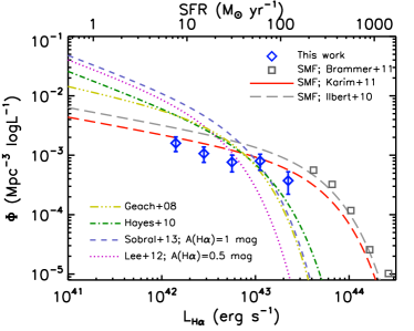
Figure 13.—  LF at $z$ = 2.24. The blue diamonds are data points based on individual extinction correction derived from SED modeling. The error bars are determined by Poisson noise. The dashed lines are the SMF of SFGs at $1.5<z<2.0$ from Ilbert et al. (2010) and that at $2.0<z<2.5$ from Karim et al. (2011). The gray squares are the SMF of SFGs at $1.8<z<2.2$ from Brammer et al. (2011). The thin lines show representative  LFs at $z=2.23$ in the literature.

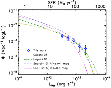
Figure 14.—  LF derived with constant extinction correction. The blue diamonds are the data points from this work. The thin lines show the  LFs from previous works with constant extinction correction: $A({\rm H\alpha})=0.5$ mag in Lee et al. (2012) and $A({\rm H\alpha})=1$ mag in other works.

6. DISCUSSION AND CONCLUSION

We have described a search for  ELGs using deep $H_{2}S1$ imaging combined with deep $K_{\mathrm{s}}$ imaging data of ECDFS. In total 140 emission-line candidates are identified. The deep optical and NIR imaging data in the ECDFS are utilized to construct broad-band SEDs and derive photo-$z$, stellar mass and extinction. We identify 56  emitters with  flux $>2.1\times 10^{-17}$ erg s^-1 cm^-1 Hz^-1. Three of the 56 are X-ray sources detected in the Chandra 4 Ms observation and two of them host an AGN in terms of their X-ray luminosities. The stacked X-ray luminosity of the rest is consistent with that of SFGs. In our sample, only $\sim$ 4% are contaminated by AGN, although obscured AGNs individually undetected in the current X-ray observation may still present in some of the sample galaxies. However, the obscured AGNs are unlikely to be responsible for exciting  line. As a result, our sample is clean for studying the properties of  ELGs and determining the  LF.

HST/ACS imaging reveals that nearly half of our  ELGs are either mergers or close pairs. A similar merger fraction was suggested by Conselice et al. (2003) for SFGs at $z\sim 2$, although large uncertainties exist in measuring merger fraction as a function of redshift (e.g., $\sim$30% for  ELGs at $z=2.23$ by Stott et al., 2013). A significant fraction (14%) of the  ELGs are too faint to be resolved in the rest-frame UV. These UV-faint ones are confirmed to be heavily-obscured SFGs by SED modeling. The remaining one third exhibit extended or compact morphologies. We note that the morphological properties of our  ELGs are consistent with those of high-$z$ SFGs (e.g., Lotz et al., 2006; Ravindranath et al., 2006; Conselice et al., 2011). Our results reveal that merging/interacting processes play a key role in regulating star formation in typical SFGs at cosmic epoch $z\sim 2-3$.

Our sample of 56  ELGs are representative of SFGs at $z\sim 2-3$ in many aspects. SFGs are found to be more obscured at higher SFR (e.g., Bothwell et al., 2011, for $z\sim 0$; Zheng et al. 2007; Ly et al. 2012; Domínguez et al. 2013 for high-$z$). We also find such a tendency among  ELGs as shown in Figure 9. Our extinction is estimated from SEDs. It is important to note that the SED-derived extinction tends to be lower than the true case represented by the IR to UV luminosity ratio $L_{\mathrm{IR}}/L_{\mathrm{UV}}$, especially at the high-SFR end (Wuyts et al., 2011a). This is understandable because in starbursts, parts of newly formed stars are deeply buried in dusty molecular clouds and can only be traced by the IR emission (e.g., Swinbank et al., 2004; Sedgwick et al., 2013). Adding this correction would enhance the correlation between extinction and SFR. The mass-SFR relation is well-established from the present day all the way to $z\sim 3$ (e.g., Elbaz et al., 2007; Daddi et al., 2007). The slope of the mass-SFR relation at $z\sim 2$ is close to unity (Wuyts et al., 2011b). As shown in Figure 10,  ELGs follow the mass-SFR relation of SFGs, giving a slope of 0.81. We argue that the shallower slope of the  ELGs is likely attributed to the underestimate of extinction at high end.

The correction for extinction on an individual basis is vital to determining the shape of the  LF. With extinction correction for individual sample galaxies, we build the  LF at $z=2.24$. The completeness as a function of  luminosity is carefully estimated via Monte Carlo simulation and is applied to the observed LF. Our sample is not large and unable to give a good constraint on the bright-end of  LF. A shallow faint-end slope of $\alpha=-1.32\pm 0.24$ is robust obtained, compared to the typical value of $\sim-1.6$ given by previous studies in which correction for a constant extinction is often adopted (Geach et al., 2008; Hayes et al., 2010; Sobral et al., 2013). We have shown that a steep faint-end slope is inevitable when a fixed extinction is applied. Garn et al. (2010) computed the  LFs at $z=0.84$ with correction for SFR-dependent extinction and constant ($A({\rm H\alpha})=1$ mag) extinction, respectively, finding that the former gives a shallower faint-end slope. It is obvious that the constant extinction correction is not a good approximation because it will overestimate the extinction in faint  ELGs and severely underestimate the extinction for brightest ones. Resolving heavily-attenuated SFGs from the emitters with faint  naturally leads to a decline at the faint end of an  LF. The extinction is broadly correlated with SFR, stellar mass, and  equivalent width (see also Garn et al., 2010; Garn & Best, 2010; Ly et al., 2012; Domínguez et al., 2013; Kashino et al., 2013). To address which parameter is more fundamental in governing extinction is beyond the scope of this work.

We argue that  LF at $z=2.24$ mirrors the SMFs of SFGs at $z\sim 2$. We know that the SED-derived extinction tends to be underestimated. Therefore, our  LF is likely underestimated too. Taking this into account, the agreement between our  LF and these converted from SMFs is notably good. The evolution of SMFs or cosmic variance may also induce additional uncertainties. We emphasize that this finding is indeed a reflection of the main sequence of SFGs. The excellent agreement between the  LF and the SMFs confirms that the main sequence has a slope close to unity. As a consequence, the -selection and the color-selection target on the same population of SFGs and naturally link the two branches of studies together.

On the other hand, the faint-end slope of  LF signifies the relative contribution between galaxies with weak and luminous , a measurement that is important to the understanding of star formation behavior over cosmic time (e.g., Dutton et al., 2010). The faint-end of an LF is shaped by processes related to star formation, e.g., feedback from supernovae (Dekel & Silk, 1986), radiatively driven winds (Springel & Hernquist, 2003), and photons ionizing neutral gas (Kravtsov et al., 2004). The dependence of the faint-end slope of  LF on extinction correction hints that UV LFs at high-$z$ might be in a similar situation. For instance, Reddy & Steidel (2009) presented the UV LF at $z\sim 2-3$ with a faint-end slope of $-1.73$. Since UV light is closely coupled with  emission, we suspect that the faint-end of the UV LF would become shallower if careful extinction correction is taken into account.

References

- An et al. (2013) An, F. X., Zheng, X. Z., Meng,Y. Z., et al. 2013, Sci China-Phys Mech Astron, 56, 2226
- Atek et al. (2010) Atek, H., Malkan, M., McCarthy, P., et al. 2010, ApJ, 723, 104
- Bertin & Arnouts (1996) Bertin, E., & Arnouts, S. 1996, A&AS, 117, 393
- Bothwell et al. (2011) Bothwell, M. S., Kenicutt, R. C., Johnson, B. D., et al. 2011, MNRAS, 415, 1815
- Brammer et al. (2008) Brammer, G. B., van Dokkum, P. G., & Coppi, P. 2008, ApJ, 686, 1503
- Brammer et al. (2011) Brammer, G. B., Whitaker, K. E., van Dokkum, P. G., et al. 2011, ApJ, 739, 24
- Brinchmann et al. (2004) Brinchmann, J., Charlot, S., White, S. D. M., et al. 2004, MNRAS, 351, 1151
- Bunker et al. (1995) Bunker, A. J., Warren, S. J., Hewett, P. C., & Clements, D. L. 1995, MNRAS, 273, 513
- Caldwell et al. (2008) Caldwell, J. A. R., McIntosh, D. H., Rix, H.-W., et al. 2008, ApJS, 174, 136
- Calzetti et al. (2000) Calzetti, D., Armus, L., Bohlin, R. C., et al. 2000, ApJ, 533, 682
- Cardamone et al. (2010) Cardamone, C. N., van Dokkum, P. G., Urry, C. M., et al. 2010, ApJS, 189, 270
- Chapman et al. (2005) Chapman, S. C., Blain, A. W., Smail, I., & Ivison, R. J. 2005, ApJ, 622, 772
- Colbert et al. (2013) Colbert, J. W., Teplitz, H., Atek, H., et al. 2013, ApJ, 779, 34
- Conselice et al. (2003) Conselice, C. J., Bershady, M. A., Dickinson, M., & Papovich, C. 2003, AJ, 126, 1183
- Conselice et al. (2011) Conselice, C. J., Bluck, A. F. L., Ravindranath, S., et al. 2011, MNRAS, 417, 2770
- Daddi et al. (2004) Daddi, E., Cimatti, A., Renzini, A., et al. 2004, ApJ, 617, 746
- Daddi et al. (2007) Daddi, E., Dickinson, M., Morrison, G., et al. 2007, ApJ, 670, 156
- Dekel & Silk (1986) Dekel, A., & Silk, J. 1986, ApJ, 303, 39
- Dickinson & FIDEL Team (2007) Dickinson, M., & FIDEL Team 2007, BAAS, 39, 822
- Domínguez et al. (2013) Domínguez, A., Siana, B., Henry, A. L., et al. 2013, ApJ, 763, 145
- Dutton et al. (2010) Dutton, A. A., van den Bosch, F. C., & Dekel, A. 2010, MNRAS, 405, 1690
- Elbaz et al. (2007) Elbaz, D., Daddi, E., Le Borgne, D., et al. 2007, A&A, 468, 33
- Erb et al. (2006b) Erb, D. K., Steidel, C. C., Shapley, A. E., et al. 2006, ApJ, 646, 107
- Fang et al. (2012) Fang, G., Kong, X., Chen, Y., & Lin, X. 2012, ApJ, 751, 109
- Fioc & Rocca-Volmerange (1997) Fioc, M., & Rocca-Volmerange, B. 1997, A&A, 326, 950
- Franx et al. (2003) Franx, M., Labbé, I., Rudnick, G., et al. 2003, ApJL, 587, L79
- Garn & Best (2010) Garn, T., & Best, P. N. 2010, MNRAS, 409, 421
- Garn et al. (2010) Garn, T., Sobral, D., Best, P. N., et al. 2010, MNRAS, 402, 2017
- Gawiser et al. (2006) Gawiser, E., van Dokkum, P. G., Herrera, D., et al. 2006, ApJS, 162, 1
- Geach et al. (2008) Geach, J. E., Smail, I., Best, P. N., et al. 2008, MNRAS, 388, 1473
- Geach et al. (2012) Geach, J. E., Sobral, D., Hickox, R. C., et al. 2012, MNRAS, 426, 679
- Grogin et al. (2011) Grogin, N. A., Kocevski, D. D., Faber, S. M., et al. 2011, ApJS, 197, 35
- Guo et al. (2013) Guo, K., Zheng, X. Z., & Fu, H. 2013, ApJ, 778, 23
- Hatch et al. (2011) Hatch, N. A., Kurk, J. D., Pentericci, L., et al. 2011, MNRAS, 415, 2993
- Hayes et al. (2010) Hayes, M., Schaerer, D., Östlin, G. 2010, A&A, 509, L5
- Hopkins & Beacom (2006) Hopkins, A. M., & Beacom, J. F. 2006, ApJ, 651, 142
- Hsieh et al. (2012) Hsieh, B.-C., Wang, W.-H., Hsieh, C.-C., et al. 2012, ApJS, 203, 23
- Ilbert et al. (2010) Ilbert, O., Salvato, M., Le Floc’h, E., et al. 2010, ApJ, 709, 644
- Karim et al. (2011) Karim, A., Schinnerer, E., Martínez-Sansigre, A., et al. 2011, ApJ, 730, 61
- Kashino et al. (2013) Kashino, D., Silverman, J. D., Rodighiero, G., et al. 2013, ApJL, 777, L8
- Kennicutt & Evans (2012) Kennicutt, R. C., & Evans, N. J. 2012, ARA&A, 50, 531
- Kennicutt (1998) Kennicutt, R. C., Jr. 1998, ARA&A, 36, 189
- Koekemoer et al. (2011) Koekemoer, A. M., Faber, S. M., Ferguson, H. C., et al. 2011, ApJS, 197, 36
- Kravtsov et al. (2004) Kravtsov, A. V., Berlind, A. A., Wechsler, R. H., et al. 2004, ApJ, 609, 35
- Kriek et al. (2009) Kriek, M., van Dokkum, P. G., Labbé, I., et al. 2009, ApJ, 700, 221
- Kroupa (2001) Kroupa, P. 2001, MNRAS, 322, 231
- Law et al. (2012) Law, D. R., Steidel, C. C., Shapley, A. E., et al. 2012, ApJ, 745, 85
- Lee et al. (2007) Lee, J. C., Kennicutt, R. C., Funes, S. J., et al. 2007, ApJ, 671, L113
- Lee et al. (2012) Lee, J. C., Ly, C., Spitler, L., et al. 2012, PASP, 124, 782
- Leitherer et al. (1999) Leitherer, C., Schaerer, D., Goldader, J. D., et al. 1999, ApJS, 123, 3
- Lotz et al. (2006) Lotz, J. M., Madau, P., Giavalisco, M., Primack, J., & Ferguson, H. C. 2006, ApJ, 636, 592
- Lotz et al. (2004) Lotz, J. M., Primack, J., & Madau, P. 2004, AJ, 128, 163
- Ly et al. (2011) Ly, C., Lee, J. C., Dale, D. A., et al. 2011, ApJ, 726, 109
- Ly et al. (2012) Ly, C., Malkan, M. A., Kashikawa, N., et al. 2012, ApJL, 747, L16
- Maraston (2005) Maraston, C. 2005, MNRAS, 362, 799
- Matsuda et al. (2011) Matsuda, Y., Smail, I., Geach, J. E., et al. 2011, MNRAS, 416, 2041
- Moorwood et al. (2000) Moorwood, A. F. M., van der Werf, P. P., Cuby, J. G., & Oliva, E. 2000, A&A, 362, 9
- Noeske et al. (2007) Noeske, K. G., Weiner, B. J., Faber, S. M., et al. 2007, ApJL, 660, L43
- Oke (1974) Oke, J. B. 1974, ApJS, 27, 21
- Papovich et al. (2005) Papovich, C., Dickinson, M., Giavalisco, M., Conselice, C. J., & Ferguson, H. C. 2005, ApJ, 631, 101
- Peng et al. (2010) Peng, Y. J., Lilly, S. J., Kovač, K., et al. 2010, ApJ, 721, 193
- Puget et al. (2004) Puget, P., Stadler, E., Doyon, R., et al. 2004, Proc. SPIE, 5492, 978
- Ravindranath et al. (2006) Ravindranath, S., Giavalisco, M., Ferguson, H. C., et al. 2006, ApJ, 652, 963
- Reddy et al. (2012) Reddy, N. A., Pettini, M., Steidel, C. C., et al. 2012, ApJ, 754, 25
- Reddy & Steidel (2009) Reddy, N. A., & Steidel, C. C. 2009, ApJ, 692, 778
- Renzini (2006) Renzini, A. 2006, ARA&A, 44, 141
- Retzlaff et al. (2010) Retzlaff, J., Rosati, P., Dickinson, M., et al. 2010, A&A, 511, A50
- Rix et al. (2004) Rix, H.-W., Barden, M., Beckwith, S. V. W., et al. 2004, ApJS, 152, 163
- Schechter (1976) Schechter, P. 1976, ApJ, 203, 297
- Sedgwick et al. (2013) Sedgwick, C., Serjeant, S., Pearson, C., et al. 2013, MNRAS, 436, 395
- Shapley (2011) Shapley, A. E. 2011, ARA&A, 49, 525
- Sobral et al. (2012) Sobral, D., Best, P. N., Matsuda, Y., et al. 2012, MNRAS, 420, 1926
- Sobral et al. (2013) Sobral, D., Smail, I., Best, P. N., et al. 2013, MNRAS, 428, 1128
- Springel & Hernquist (2003) Springel, V., & Hernquist, L. 2003, MNRAS, 339, 312
- Steidel et al. (1999) Steidel, C. C., Adelberger, K. L., Giavalisco, M., Dickinson, M., & Pettini, M. 1999, ApJ, 519, 1
- Stott et al. (2013) Stott, J. P., Sobral, D., Smail, I., et al. 2013, MNRAS, 430, 1158
- Swinbank et al. (2004) Swinbank, A. M., Smail, I., Chapman, S. C., et al. 2004, ApJ, 617, 64
- van Dokkum et al. (2011) van Dokkum, P. G., Brammer, G., Fumagalli, M., et al. 2011, ApJL, 743, L15
- Wang et al. (2010) Wang, W.-H., Cowie, L. L., Barger, A. J., Keenan, R. C., & Ting, H.-C. 2010, ApJS, 187, 251
- Wuyts et al. (2011a) Wuyts, S., Förster Schreiber, N. M., Lutz, D., et al. 2011, ApJ, 738, 106
- Wuyts et al. (2011b) Wuyts, S., Förster Schreiber, N. M., van der Wel, A., et al. 2011, ApJ, 742, 96
- Xue et al. (2011) Xue, Y. Q., Luo, B., Brandt, W. N., et al. 2011, ApJS, 195, 10
- Yan et al. (1999) Yan, L., McCarthy, P. J., Freudling, W., et al. 1999, ApJ, 519, L47
- Zheng et al. (2006) Zheng, X. Z., Bell, E. F., Rix, H.-W., et al. 2006, ApJ, 640, 784
- Zheng et al. (2007) Zheng, X. Z., Dole, H., Bell, E. F., et al. 2007, ApJ, 670, 301