From Filaments to Oscillating Starless Cores

Abstract

Long wavelength sonic oscillations are observed or inferred in many of the small, dark molecular clouds, the starless cores, that are the precursors to protostars. The oscillations provide significant internal energy and the time scale for their dissipation may control the rate of star formation in starless cores. Despite their importance, their origin is unknown. We explore one hypothesis that the oscillations develop as a starless core forms from a filament. We model this process with a numerical hydrodynamic simulation and generate synthetic molecular line observations with a radiative transfer simulation. Comparison with actual observations shows general agreement suggesting the proposed mechanism is viable.

1 Introduction

In this paper we explore an hypothesis that the kinetic energy associated with the sonic oscillations observed in starless cores comes from the gravitational energy released as a core forms from a filament by gravitational contraction.

The starless cores are dense concentrations of a few solar masses of molecular gas and are commonly observed in low-mass star-forming regions such as Taurus and Ophiucus (di Francesco et al., 2007; André et al., 2013). They are significant as the future birthplaces of stars of one-half to a few solar masses, the most common stars in the galaxy (Myers & Benson, 1983; Beichman et al., 1986). Their internal oscillations are significant because they may control the evolution toward star formation. In star-forming regions such as Taurus, many starless cores are massive and dense enough that their internal thermal energy provides only about 70% of the energy needed for stability against gravitational collapse (Dickman & Clemens, 1983; Myers & Benson, 1983; Evans et al., 2001; Kandori et al., 2005; Kirk, Ward-Thompson & André, 2005). The remaining energy required for stability may be in the kinetic energy of the oscillations (Keto et al., 2006; Broderick & Keto, 2010).

If oscillations support the cores, then the dissipation of the oscillations by mode-mode coupling and radiation should result in gravitational collapse and star formation if the oscillation energy is not resupplied (Broderick & Keto, 2010). In this case, the core lifetimes would be equal to the dissipation time (Broderick et al., 2008). This deduction is supported by some observations that suggest that more evolved cores, those with newly formed stars, have less turbulent energy than the starless cores (Tachihara et al., 2002).

Statistical arguments based on observation suggest that most cores have lifetimes longer than their free-fall times (Beichman et al., 1986; Jessop & Ward-Thompson, 2000; Ward-Thompson et al., 2007). If many cores require additional energy for stability, and the oscillations are the source of that energy, then the core lifetimes suggest that many cores are oscillating, not just the few observed with complex modes (Lada et al., 2003; Redman, Keto & Rawlings, 2006; Aguti et al., 2007).

Despite the possible significance of the oscillations in the evolution of star-forming cores, the origin of the oscillations and the source of their energy is unknown. Keto & Field (2005) supposed that the oscillations were the expression of the subsonic turbulence at the bottom of the supersonic turbulent cascade that characterizes the velocities in the larger-scale interstellar medium (Field, Blackman & Keto, 2011). However, they did not specify further. Similarly, Broderick & Keto (2010) assumed an initial turbulent spectrum, either Kolmogoroff or flat, but again without specfiying the origin.

The origin of the oscillations may be in the process of core formation from filaments. As a filament fragments and contracts to form a spherical core, the gravitational energy released is converted into kinetic energy in oscillations. This hypothesis is motivated by both observation and theory. Observations of low-mass star-forming regions show that the cores are often associated with filaments (Goldsmith et al., 2008; Myers, 2009). Theoretically, we know that self-gravitating filaments are unstable to fragmentation and the formation of cores. It may be that most cores form out of filaments.

We model the process of core formation from the contraction of a filamentary fragment with a hydrodynamic simulation. We follow the evolution and at various time we simulate observable spectral lines that can be compared with actual observations. We find that in the initial contraction, the velocities are mostly linear, along the filament, in the direction of the contraction. As the gas rebounds off its own thermal pressure, the fragment flattens and expands perpendicular to the length of the initial filament. This is followed by a long period of oscillations of slowly decreasing amplitude. Eventually the velocities become more and more radial as the fragment becomes more and more spherical.

The profiles of the simulated spectral lines are generally consistent with those observed. Our conclusion is that this is a plausible hypothesis for the generation of the oscillations in starless cores.

2 Numerical hydrodynamic simulation

We use the smoothed-particle hydrodynamic code of Wetzstein et al. (2009) and follow the method of simulation as described in Burkert & Alves (2009). We begin the evolution with a finite cylinder to represent a fragment of a filament. We set the mass of the filamentary fragment to 3 M_⊙ and the sound speed of the molecular gas to 0.2 km s^-1 corresponding to a gas temperature of 12 K.

We know that if the fragment is bounded by an external pressure it will evolve to a sphere in hydrostatic equilibrium, a Bonnor-Ebert (BE) sphere (Bonnor, 1956). We want the final configuration to be stable against gravitational collapse so we choose the external pressure, which is constant throughout the simulation, to be just below the pressure for critical stability of a sphere that is the same mass and isothermal temperature as the initial cylindrical fragment. More precisely, we set the external pressure to the critical value for the stability of a (BE) sphere slightly more massive (3.4 M_⊙) than our filamentary fragment. In the simulation, confinement by an external pressure is simulated as, $P=\rho/c_{s}^{2}-P_{ext}$ applied to all particles (see Burkert & Alves, 2009).

With the mass, sound speed, and external pressure defined, it remains to set the initial configuration of the filamentary fragment. The hydrostatic configuration for a pressure-bounded cylinder of infinite length (Ostriker, 1964; Fischera & Martin, 2012) is not completely appropriate because our filament has a finite length. We therefore start with a filament with a uniform density $1\times 10^{-20}$ g cm^-3 and let it relax in the radial direction suppressing all gas motion along the long axis (X-axis). The filamentary fragment evolves to a hydrostatic solution that is taken as the initial condition for the subsequent simulation. The axial ratio of the filamentary fragment is 3:1.

The SPH simulations were run with 80K equal-mass particles, fulfilling the resolution requirement of Bate & Burkert (1997). The SPH smoothing length should be a fraction of the dynamical and structural size scales. It depends on the local density and in our clouds is of order 5% of the mean radius. The dominant oscillations are on length scales that are a factor of 5 to 10 larger and are therefore well resolved. The resolution was also tested by comparison with a simulation of half as many particles.

3 Radiative transfer

We use the 3D non-LTE radiative transfer code MOLLIE (Keto, 1990; Keto & Rybicki, 2010) to produce simulated spectral lines as would be seen in a mm-wavelength radio observation. The abundance of the molecular species is determined with a simple chemical model as described in Keto & Caselli (2008, 2010) that includes the effects of freeze-out at high density in the core or filament center and photodissociation near the boundary. We produced radiative transfer simulations for CO, CS, HCO⁺, and N₂H⁺. Owing to the low mass and low optical depth of the core, the spectral signatures of all the molecules were similar despite their differing optical depths and critical densities for collisional de-excitation. We show only the results for HCO⁺ in the figures in this paper.

4 Results

The initial state of the filament is out of equilibrium longitudinally because of the truncation to a fragment. The momentum of the initial longitudinal contraction along X causes the filament to flatten perpendicular to X and expand in a disk shape along the YZ plane. Figure 1 shows the XY and YZ projections of the fragment at this time (2.2 Myr). The outer part of the flattened fragment is expanding, rebounding from the longitudinal contraction while the inner part is radially contracting.

The two perpendicular motions, longitudinal and radial, continue to oscillate between contraction and expansion with different periods, creating complex patterns of velocities and densities (figures 4 through 9) even though the initial state is highly symmetric. For example, in figure 4, the gas density is highest in a ring around the core center. The brightness of the spectral lines in figure 6 is correspondingly lower in the center. This shows how oscillations can create peaks in the column density that are located away from the core center. Off-center column density peaks are commonly seen in the simulations of fully turbulent cores (Broderick & Keto, 2010).

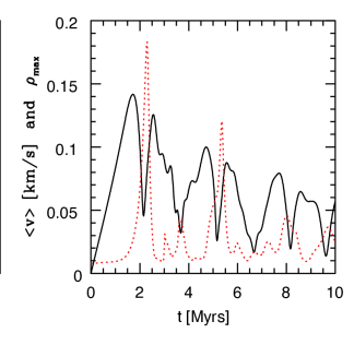
Figure 10: Average velocity (black solid line)and maximum density (red dotted line) as a function of time. The average velocity is defined by the total kinetic energy, $E_{kin}$ divided by the total mass, $M$, $v=\sqrt{2*E_{kin}/M}$. The units of density are $2\times 10^{-18}$ g cm^-3. The figure shows the 2 periods of oscillation, longitudinal and radial with the highest densities occurring at the point of maximum compression when the velocities are low and reversing.

The simulation shows continuous damping of the velocities or amplitudes of the oscillations. Figure 10 shows the average velocity defined by the total kinetic energy, $E_{kin}$ divided by the total mass, $M$, $v=\sqrt{2*E_{kin}/M}$. The average velocity decreases by a factor of 3 over a time scale of 10 Myr. In late phases, the typical oscillation velocity is of order 0.03 - 0.05 km/s which is of order 20-30% the sound speed. The principle damping mechanism is by non-linear coupling between the modes which is a decrease in momentum caused by collisions between fluid streams. In comparison to the wave damping time, the free-fall and crossing times are approximately 0.5 Myr. The figure also shows the maximum density in the fragment which occurs in each cycle at the point of maximum compression when the velocities are low and reversing. The effect of the two different periods, longitudinal and radial, is seen in this figure. An animation of the oscillating filament may be seen at http://www.usm.uni-muenchen.de/people/burkert/filament/index.html.

The velocities are subsonic throughout the simulation resulting in asymmetric rather than split spectral line profiles. The simulated spectral lines seen in an observation on a viewing angle perpendicular to long axis of the filament (figure 2) are dominated by the outer regions of the fragment and show the signature of expansion with the red side of the asymmetric line profile brighter than the blue side. The red asymmetry of the spectral line (figure 2 right) is also seen as red in the first moment map (figure 2 left). On a view parallel with the filament, the spectra form a more complex pattern where the line profiles are asymmetrical blue and then red in alternating zones. Complex patterns of asymmetric spectral lines such as this that cannot be created by any combination of rotation and either expansion or contraction and have been suggested to be an indication of oscillations (Lada et al., 2003).

The simulated spectral line profiles in figures 2 (right) through 9 (right) may be compared with actual observations, for example, figure 6 of Lada et al. (2003), figure 3 of Redman, Keto & Rawlings (2006), and figure 2 of Aguti et al. (2007).

5 Discussion

This paper discusses one possible mechanism for the origin of the oscillations as a core forms from a filament. Part of the motivation for this hypothesis is the difficulty of other means. Excitation of the oscillations by external forces may not be trivial. If two starless cores pass near each other, the time scale of the encounter needs to be about equal to the internal sound-crossing time for the core to be tidally excited. This requires a particular relative velocity. If two cores merge rather than pass each other, the collision has to be slow enough that both cores are not disrupted. The combined mass of the merger also has to be low enough that the resulting core is stable against gravitational collapse. For example, Burkert & Alves (2009) considered whether the present state of the core B68 were due to a merger. They concluded that if so, the main core which now appears stable, would soon collapse with the additional mass of the companion. The problem with external excitation of the oscillations is that if both passing encounters and mergers require special conditions then these mechanisms would not be suitable to supply oscillation energy to many or most cores. In contrast, the mechanism for the origin of the oscillations in the origin of the cores is universal.

We have not addressed the origin of our initial state, the filamentary fragments, or why that state should be such as to form a stable starless core. Filaments and cores are common and intimate in low-mass star-forming regions. Self-gravitating filaments are unstable to longitudinal fragmentation on the scale of a Jeans length. This scale would produce cores with a Jeans mass, similar to the critically stable mass.

With our highly idealized and symmetric initial state, we cannot properly address the stability of the cores during their formation. The reason is that from our choice of initial state, the initial longitudinal contraction is destabilizing, similar to the breathing mode in a spherical cloud defined as the (0,0,0) mode in radial and spherical harmonics . In breathing mode oscillations, the inward momentum in the compressive phase acts like an additional external pressure and may squeeze an otherwise stable, self-gravitating cloud past its point of stability and cause it to collapse rather than rebound. In contrast, oscillations with higher order modes are stabilizing. We would need more complex initial states to investigate stability. For example, Broderick & Keto (2010) assumed fully turbulent cores in their analysis of stability, but this already assumes the oscillations whose origins we seek to explain.

Nothing requires that all cores form in a stable state. For example, star forming regions such as Taurus are defined by a high star formation rate indicating a large number of unstable cores. Many of these star-forming cores could have been unstable from formation. The energy in oscillations may help explain why there are currently a large number of cores that otherwise appear to be unstable and why the core lifetimes are statistically longer than their free-fall times.

Magnetic fields, not included in our simulation, could affect the evolution of the cloud (Hennebelle, 2003; Galli, 2005). We assume that the magnetic energy is in equipartition with the kinetic energy. Since most of the energy in observed clouds is thermal, the magnetic energy should be a minor contributor. If the gas velocities in filaments prior to contraction are turbulent (subsonic) then the field should also be disordered. In this case the effect of the field may be approximated as an additional pressure. However, if the field were ordered and anchored on larger scales, the geometry of the initial filament could be quite different depending on the geometry of the field.

6 Conclusions

A hydrodynamic simulation of a contracting filamentary fragment is able to produce oscillating cores with some complexity despite the high degree of symmetry in our choice of initial state. The general agreement between simulated and actual spectral line observations maintains the viability of this mechanism for the origin of the oscillations.

$\begin{array}[]{cc}\includegraphics[trim=7.22743pt 361.34999pt 57.81621pt 36.135pt,clip,width=234.87749pt]{fnewxy-2p157}\includegraphics[trim=7.22743pt 361.34999pt 57.81621pt 36.135pt,clip,width=234.87749pt]{fnewyz-2p157}\end{array}$

Figure 1: Densities and velocities on slices through two orientations at 2.2 Myr, (left) in the XY plane at Z=0, and (right) in the YZ planet X=0. The filament was originally aligned with the X-axis. The axes are labeled in units of $10^{17}$ cm and the density in units of $2\times 10^{-18}$ g cm^-3. The longest arrow, the largest velocity is 0.62 km s^-1.

$\begin{array}[]{cc}\includegraphics[trim=7.22743pt 397.48499pt 57.81621pt 72.26999pt,clip,width=234.87749pt,angle={180}]{fig2Lnew}\includegraphics[trim=7.22743pt 115.63243pt 57.81621pt 28.90755pt,clip,width=234.87749pt,angle={180}]{fig2R}\end{array}$

Figure 2: (Left) First moment of the simulated HCO⁺(1-0) line on a projection along the Z axis. The axes are labeled in arc minutes assuming a distance of 250 pc. Velocities in km s^-1. (Right) Spectra at intervals of 0.42 arc minutes. The velocity axis spans a range of -1 to +1 km s^-1. The maximum brightness is 3.5 K.

$\begin{array}[]{cc}\includegraphics[trim=7.22743pt 397.48499pt 57.81621pt 72.26999pt,clip,width=234.87749pt,angle={180}]{fig3Lnew}\includegraphics[trim=7.22743pt 115.63243pt 57.81621pt 28.90755pt,clip,width=234.87749pt,angle={180}]{fig3R}\end{array}$

Figure 3: Same as figure 2 but on a projection on the YZ axis. The maximum brightness is 4.6 K.

$\begin{array}[]{cc}\includegraphics[trim=7.22743pt 361.34999pt 57.81621pt 36.135pt,clip,width=234.87749pt]{fig4Lnew}\includegraphics[trim=7.22743pt 361.34999pt 57.81621pt 36.135pt,clip,width=234.87749pt]{fig4Rnew}\end{array}$

Figure 4: Same as figure 1 except for a time of 2.9 Myr. The maximum velocity is 0.17 km s^-1.

$\begin{array}[]{cc}\includegraphics[trim=7.22743pt 397.48499pt 57.81621pt 72.26999pt,clip,width=234.87749pt,angle={180}]{fig5Lnew}\includegraphics[trim=7.22743pt 115.63243pt 57.81621pt 72.26999pt,clip,width=234.87749pt,angle={180}]{fig5R}\par\end{array}$

Figure 5: Same as figure 2 but for a time of 2.7 Myr. The maximum brightness in the spectra is 0.5 K.

$\begin{array}[]{cc}\includegraphics[trim=7.22743pt 397.48499pt 57.81621pt 72.26999pt,clip,width=234.87749pt,angle={180}]{fig6Lnew}\includegraphics[trim=7.22743pt 122.85876pt 57.81621pt 72.26999pt,clip,width=234.87749pt,angle={180}]{fig6R}\end{array}$

Figure 6: Same as figure 5 but on a projection on the YZ axis. The maximum brightness is 0.6 K

$\begin{array}[]{cc}\includegraphics[trim=7.22743pt 361.34999pt 57.81621pt 36.135pt,clip,width=234.87749pt]{fig7Lnew}\includegraphics[trim=7.22743pt 361.34999pt 57.81621pt 36.135pt,clip,width=234.87749pt]{fig7Rnew}\end{array}$

Figure 7: (figxy-3p448) Same as figure 1 except for a time of 3.4 Myr. The maximum velocity is 0.08 km s^-1.

$\begin{array}[]{cc}\includegraphics[trim=7.22743pt 397.48499pt 57.81621pt 72.26999pt,clip,width=234.87749pt,angle={180}]{fig8Lnew}\includegraphics[trim=7.22743pt 122.85876pt 57.81621pt 72.26999pt,clip,width=234.87749pt,angle={180}]{fig8R}\end{array}$

Figure 8: Same as figure 2 but for a time of 3.5 Myr. The maximum brightness in the spectra is 0.8 K.

$\begin{array}[]{cc}\includegraphics[trim=7.22743pt 397.48499pt 57.81621pt 72.26999pt,clip,width=234.87749pt,angle={180}]{fig9Lnew}\includegraphics[trim=7.22743pt 122.85876pt 57.81621pt 72.26999pt,clip,width=234.87749pt,angle={180}]{fig9R}\par\end{array}$

Figure 9: Same as figure 8 but on a projection on the YZ axis. The maximum brightness is 0.8 K.

Acknowledgements A.B. thanks the Harvard-Smithsonian Center for Astrophysics for their hospitality during multiple visits. The research of A.B. is supported by the priority program 1573 ”Physics of the Interstellar Medium” of the German Science Foundation.

References

- Aguti et al. (2007) Aguti E. D., Lada C. J., Bergin E. A., Alves J. F., Birkinshaw M., 2007, ApJ, 665, 457
- André et al. (2013) André P., Di Francesco J., Ward-Thompson D., Inutsuka S.-i., Pudritz R. E., Pineda J., 2013, ArXiv e-prints
- Bate & Burkert (1997) Bate M. R., Burkert A., 1997, MNRAS, 288, 1060
- Beichman et al. (1986) Beichman C. A., Myers P. C., Emerson J. P., Harris S., Mathieu R., Benson P. J., Jennings R. E., 1986, ApJ, 307, 337
- Bonnor (1956) Bonnor W. B., 1956, MNRAS, 116, 351
- Broderick & Keto (2010) Broderick A. E., Keto E., 2010, ApJ, 721, 493
- Broderick et al. (2008) Broderick A. E., Narayan R., Keto E., Lada C. J., 2008, ApJ, 682, 1095
- Burkert & Alves (2009) Burkert A., Alves J., 2009, ApJ, 695, 1308
- di Francesco et al. (2007) di Francesco J., Evans, II N. J., Caselli P., Myers P. C., Shirley Y., Aikawa Y., Tafalla M., 2007, in Protostars and Planets V, Reipurth B., Jewitt D., K. K., eds., University of Arizona Press: Tuscon, pp. 17–32
- Dickman & Clemens (1983) Dickman R. L., Clemens D. P., 1983, ApJ, 271, 143
- Evans et al. (2001) Evans, II N. J., Rawlings J. M. C., Shirley Y. L., Mundy L. G., 2001, ApJ, 557, 193
- Field, Blackman & Keto (2011) Field G. B., Blackman E. G., Keto E. R., 2011, MNRAS, 416, 710
- Fischera & Martin (2012) Fischera J., Martin P. G., 2012, A&A, 542, A77
- Galli (2005) Galli D., 2005, MNRAS, 359, 1083
- Goldsmith et al. (2008) Goldsmith P. F., Heyer M., Narayanan G., Snell R., Li D., Brunt C., 2008, ApJ, 680, 428
- Hennebelle (2003) Hennebelle P., 2003, A&A, 411, 9
- Jessop & Ward-Thompson (2000) Jessop N. E., Ward-Thompson D., 2000, MNRAS, 311, 63
- Kandori et al. (2005) Kandori R. et al., 2005, AJ, 130, 2166
- Keto et al. (2006) Keto E., Broderick A., Lada C. J., Narayan R., 2006, ArXiv Astrophysics e-prints
- Keto & Caselli (2008) Keto E., Caselli P., 2008, ApJ, 683, 238
- Keto & Caselli (2010) Keto E., Caselli P., 2010, MNRAS, 402, 1625
- Keto & Field (2005) Keto E., Field G., 2005, ApJ, 635, 1151
- Keto & Rybicki (2010) Keto E., Rybicki G., 2010, ApJ, 716, 1315
- Keto (1990) Keto E. R., 1990, ApJ, 355, 190
- Kirk, Ward-Thompson & André (2005) Kirk J. M., Ward-Thompson D., André P., 2005, MNRAS, 360, 1506
- Lada et al. (2003) Lada C. J., Bergin E. A., Alves J. F., Huard T. L., 2003, ApJ, 586, 286
- Myers (2009) Myers P. C., 2009, ApJ, 700, 1609
- Myers & Benson (1983) Myers P. C., Benson P. J., 1983, ApJ, 266, 309
- Ostriker (1964) Ostriker J., 1964, ApJ, 140, 1056
- Redman, Keto & Rawlings (2006) Redman M. P., Keto E., Rawlings J. M. C., 2006, MNRAS, 370, L1
- Tachihara et al. (2002) Tachihara K., Onishi T., Mizuno A., Fukui Y., 2002, A&A, 385, 909
- Ward-Thompson et al. (2007) Ward-Thompson D., André P., Crutcher R., Johnstone D., Onishi T., Wilson C., 2007, Protostars and Planets V, 33
- Wetzstein et al. (2009) Wetzstein M., Nelson A. F., Naab T., Burkert A., 2009, ApJ Suppl, 184, 298