Zero-Determinant Strategies in the Iterated Public Goods Game

Abstract

Recently, Press and Dyson have proposed a new class of probabilistic and conditional strategies for the two-player iterated Prisoner’s Dilemma, so-called zero-determinant strategies. A player adopting zero-determinant strategies is able to pin the expected payoff of the opponents or to enforce a linear relationship between his own payoff and the opponents’ payoff, in a unilateral way. This paper considers zero-determinant strategies in the iterated public goods game, a representative multi-player evolutionary game where in each round each player will choose whether or not put his tokens into a public pot, and the tokens in this pot are multiplied by a factor larger than one and then evenly divided among all players. The analytical and numerical results exhibit a similar yet different scenario to the case of two-player games: (i) with small number of players or a small multiplication factor, a player is able to unilaterally pin the expected total payoff of all other players; (ii) a player is able to set the ratio between his payoff and the total payoff of all other players, but this ratio is limited by an upper bound if the multiplication factor exceeds a threshold that depends on the number of players.

I Introduction

Iterated games have long been exemplary models for the emergence of cooperations in socioeconomic and biological systems Axelrod1981 ; Axelrod1984 ; Axelrod1988 ; Nowak1993 ; Nowak2006 ; Kendall2007 . Learned from these studies, the most significant lesson is that in the long term, selfish behavior will hurt you as much as your opponents. Therefore, from both scientific and moral perspectives, ants and us all live in a reassuring world: altruists will eventually dominate a reasonable population. Very recently, however, Press and Dyson Press2012 have shattered this well-accepted scenario by introducing a new class of probabilistic memory-one strategies for the two-player iterated Prisoner’s Dilemma (IPD), so-called zero-determinant (ZD) strategies. Via ZD strategies, a player can unilaterally pin his opponents’ expected payoff or extort his opponents by enforcing a linear relationship between his own payoff and the opponents’ payoff. In a word, egotists could become more powerful and harmful if they know mathematics. Though being challenged by the evolutionary stability Adami2013 ; Hilbe2013 ; Stewart2013 , studies on ZD strategies as a whole Press2012 ; Adami2013 ; Hilbe2013 ; Stewart2013 ; Akin2012 ; Chen2013 ; Hilbe2013b ; Daoud2014 ; Szolnoki2014 will dramatically change our understanding on iterated games Stewart2012 ; Hayes2013 . Indeed, knowing the existence of ZD strategies has already changed the game.

ZD strategies in IPD can be naturally extended to other iterated two-player games Roemheld2013 , which are still uncultivated lands for scientists. Instead, we turn our attention to the iterated multi-player games and try to answer a blazing question: could a single ZD player in a group of considerable number of players unilaterally pin the expected total payoff of all other players and extort them? This paper focuses on a notable representative of multi-player games, the public goods game (PGG) Hardin1968 ; Kagel1995 . In the simplest $N$-player PGG, each player chooses whether or not contribute a unit of cost into a public pot. The total contribution in the public pot will be multiplied by a factor $r$ ($1<r<N$) and then be evenly divided among all $N$ players, regardless whether they have contributed or not. As a simple but rich model, the PGG arises a question why and when a player is willing to contribute against the obvious Nash equilibrium at zero Fehr2003 , which is critical for the understanding, predicting and intervening of many important issues ranging from micro-organism behaviors Cordero2012 ; Bachmann2013 to global warming Milinski2006 ; Milinski2008 ; Tavonia2011 ; Santos2011 . Among a couple of candidates SigmundPNAS01 ; Hauert2002 ; SzaboPRL2002 ; Santos2008 ; RongPRE2010 ; Apicella2012 ; Perc2013 , the repeated interactions may be a relevant mechanism to the above question, since reputation, trustiness, reward and punishment can then play a role Fehr2000 ; Milinski2002 . We thus study the iterated public goods game (IPGG, also named as repeated public goods game in the literatures) where the same players in a group play a series of stage games.

It is found by surprise that the ZD strategies still exist for a group with many players in IPGG, namely a single player can pin the total payoff of all others or extort them in a unilateral way. However, different from the observations in IPD, there exists some unreported restrictive conditions related to the group size and multiplication factor, which determine the feasibility to pin the total payoff of all other players and the upper bound of extortionate ratio.

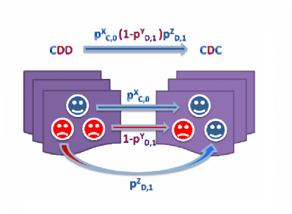
(a)

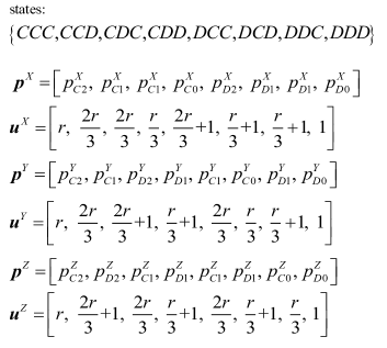
(b)

(c)

(d)

Figure 1: Illustration of the general three-player game. (a) For a previous state $CDD$, the conditional probabilities that the players $X$, $Y$ and $Z$ select $C$ in the current round are $p^{X}_{C,0}$, $p^{Y}_{D,1}$ and $p^{Z}_{D,1}$, respectively. Therefore, the probability from the previous state $CDD$ to the current state $CDC$ is $p^{X}_{C,0}(1-p^{Y}_{D,1})p^{Z}_{D,1}$. (b) shows the $2^{3}=8$ different states, the strategy vectors and payoff vectors of the three players. According to Eq. (4) and Eq. (5), the Markov transition matrix M for the present case is shown in (c). After some elementary column operations on matrix $\bf{M-I}$, the dot product of an arbitrary vector $\bf{u}$ with the stationary vector $\bf{v}$ is equal to the determinant $\det({{\bf{p}}^{X}},{{\bf{p}}^{Y}},{{\bf{p}}^{Z}},{\bf{u}})$ as shown in (d), where ${\bf{\tilde{p}}}^{X}$, ${\bf{\tilde{p}}}^{Y}$ and ${\bf{\tilde{p}}}^{Z}$ lie in the forth, sixth and seventh columns which are only controlled by the players $X$, $Y$ and $Z$, respectively.

II ZD Strategies in Multi-Player Games

Consider an $N$-player iterated game, which consists of a series of repetitions of a same stage game of $N$ players. Press and Dyson Press2012 proved the theorem that, in such an iterated game, if the stage games are identically repeated infinite times, a long-memory player will have no advantage over a short-memory player. Without loss of generality, it is suffice to derive players’ strategy assuming they have only memory-one. Thus, which action a player will take in the current round depends on the outcome of the previous round. For an arbitrary player $X\in\{1,2,\cdots,N\}$, a (mixed) strategy ${\bf{p}}^{X}$ is a vector that consists of conditional probabilities for cooperating with respect to every possible outcome. Since we consider a general $N$-player game and every player may choose cooperation ($C$) or defection ($D$), there are $2^{N}$ possible outcomes for each round. For player $X$, his memory-one strategy can be represented by a $2^{N}$-dimensional vector:

$$\begin{split}{\bf{p}}^{X}=&\left[p^{X}_{1},\ \cdots\ \,p^{X}_{i},\ \cdots\ \,p^{X}_{2^{N}}\right]^{T},\end{split}$$ (1)

where $p^{X}_{i}$ stands for the conditional probability that $X$ will cooperate in the current round, given the outcome of the previous round. Here $i{\small{=}}1,2,\cdots,2^{N}$ is the index of possible outcomes in each round. Figure 1 shows an example for an $N{\small{=}}3$ game, in which the players are $X$, $Y$ and $Z$, and the possible outcomes are $\{CCC,CCD,CDC,CDD,DCC,DCD,DDC,DDD\}$.

In many multi-player games such as public goods game Hardin1968 ; Kagel1995 , N-player snowdrift game ZhengEPL07 , N-player stag-hunt game PachecoPRSB09 and collective-risk social dilemma Milinski2008 , whether a specific opponent chooses to cooperate is less meaningful, instead, it is crucial for a player to know how many his opponents cooperate. In such a scenario, if a player $X$’s previous move is $C$ and the number of cooperators among the opponents in the previous round is $n\in\{0,1,\cdots,N-1\}$, the probabilities for him to cooperate in the current round are denoted as $p^{X}_{C,n}$. Similarly, if his previous move is $D$ and the number of cooperating opponents is $n$, the probability to cooperate is $p^{X}_{D,n}$. Therefore, the original strategy vector in Eq. (1) can be refined to a $2^{N}$-dimensional vector with $2N$ independent variables as:

$$\begin{split}{\bf{p}}^{X}=&[p^{X}_{C,0},\ \cdots\ ,\underbrace{p^{X}_{C,n},\cdots\,p^{X}_{C,n}}_{\binom{N-1}{n}\ terms}\ ,\cdots\ ,p^{X}_{C,N-1},\\ &p^{X}_{D,0},\ \cdots\ ,\underbrace{p^{X}_{D,n},\cdots\,p^{X}_{D,n}}_{\binom{N-1}{n}\ terms}\ ,\cdots,\ p^{X}_{D,N-1}]^{T}.\end{split}$$ (2)

Figure 1(b) gives an example of the strategy vectors for the three-player case.

Starting at an initial outcome, the $N$ players’ strategy profile determines a stochastic process. Since these are memory-one strategies, the corresponding stochastic process can be characterized by a Markov chain. Each possible outcome of the repeated games can be maintained by a state in this Markov chain model. Under this model, the state transition rules are joint probabilities calculated from the $N$ players’ probabilistic strategies. Denoting the corresponding transition matrix as:

$$\begin{split}{\bf{M}}=\left[M_{ij}\right]_{{2^{N}}\times{2^{N}}},\end{split}$$ (3)

where the element $M_{ij}$ is a one-step transition probability of moving from state $i$ to state $j$. It is essentially a joint probability that can be calculated as:

$$M_{ij}=\prod\nolimits_{X=1}^{N}m^{X},$$ (4)

where $X$ runs over all players, and

$$m^{X}=\left\{\begin{array}[]{l}(p_{C,n(i)}^{X})^{h_{j}^{X}}(1-p_{C,n(i)}^{X})^{1-h_{j}^{X}},{\textrm{ if $X$ takes $C$ in state $i$}};\\ (p_{D,n(i)}^{X})^{h_{j}^{X}}(1-p_{D,n(i)}^{X})^{1-h_{j}^{X}},{\textrm{if $X$ takes $D$ in state $i$}}.\\ \end{array}\right.$$ (5)

Here $n(i)$ is the number of cooperators among $X$’s opponents in state $i$. $h_{j}^{X}$ is an indicator, a binary variable determined by player $X$’s action in state $j$. Conventionally, if player $X$’s action in state $j$ is $C$, then $h_{j}^{X}=1$; otherwise, $h_{j}^{X}=0$. Figure 1(c) shows $\bf{M}$ for the general three-player game. It can be easily checked that the sum of each row equals $1$.

In Eq. (4) and Eq. (5), the transition probabilities are dependent on all the $N$ players’ strategies, reflecting the complexity of the multi-player games. However, the approach proposed by Press and Dyson Press2012 allow us to derive a class of strategies succinctly, but profoundly. Define a matrix ${\bf{M}}^{\prime}={\bf{M-I}}$, where ${\bf{I}}$ is the unit diagonal matrix. After some elementary column operations on this matrix, the joint probabilities will be finely separated, leaving one column solely controlled under player $X$’s strategy but not dependent on other players anymore. This column $\tilde{\bf{p}}^{X}$ is shown as follows:

$$\begin{split}{\tilde{\bf{p}}^{X}}=&[-1+p^{X}_{C,0},\ \cdots\ ,\underbrace{-1+p^{X}_{C,n},\cdots\ ,-1+p^{X}_{C,n}}_{\binom{N-1}{n}\ terms}\ ,\cdots\ \\ &-1+p^{X}_{C,N-1},\ p^{X}_{D,0},\ \cdots\ ,\underbrace{p^{X}_{D,n},\cdots\ ,p^{X}_{D,n}}_{\binom{N-1}{n}\ terms}\ ,\\ &\cdots\ ,p^{X}_{D,N-1}]^{T}.\end{split}$$ (6)

In Eq. (6), all the probabilities depend only on the elements in Eq. (2), which indicates that ${\bf{\tilde{p}}}^{X}$ is unilaterally controlled by player $X$. Note that ${\bf{\tilde{p}}}^{X}$ is a $2^{N}$-dimensional vector, and the elements $-1+p_{C,n}^{X}$ and $p_{D,n}^{X}$ each appears $\binom{N-1}{n}$ times. Figure 1(d) gives an example of the unilateral control for the general three-player game. We can see that the forth, sixth and seventh columns in this matrix only involve the strategies of players $X$, $Y$ and $Z$, respectively.

If the transition matrix $\bf{M}$ is regular, i.e., the Markov chain is irreducible and aperiodic, it will be ensured that there exists a stationary probability vector ${\bf{v}}$, such that

$$\begin{array}[]{l}{{\bf{v}}^{T}}\cdot{\bf{M}}={{\bf{v}}^{T}}.\end{array}$$ (8)

The stationary vector ${\bf{v}}$ is the very eigenvector corresponding to the eigenvalue ${\bf{1}}$ of M. Press and Dyson  Press2012 prove that, there is a proportional relationship between the stationary vector $\bf{v}$ and each row in the adjugate matrix ${\mathrm{Adj}}({\bf{M}}^{\prime})$, which links the stationary vector and the determinant of transition matrix, such that:

$$\begin{array}[]{l}{\bf{v}}^{T}\cdot{\bf{u}}=\det({{\bf{p}}^{1}},\cdots,{{\bf{p}}^{X}},\cdots,{{\bf{p}}^{N}},{\bf{u}}),\end{array}$$ (10)

where $({{\bf{p}}^{1}},\cdots,{{\bf{p}}^{X}},\cdots,{{\bf{p}}^{N}},{\bf{u}})$ is a $2^{N}\times 2^{N}$ determinant and ${\bf{u}}$ is the last column of ${\bf{M}}^{\prime}$. This theorem is of much significance since it allows us to calculate one player’s long-term expected payoff by using the Laplace expansion on the last column of ${\bf{M}}^{\prime}$. Let ${{\bf{u}}^{X}}$ denote the payoff vector for the player $X$. Replacing the last column of ${\bf{M}}^{\prime}$ by ${{\bf{u}}^{X}}$, we can calculate player $X$’s long-term expected payoff as:

$$\begin{split}E^{X}=\frac{\det({{\bf{p}}^{1}},\cdots,{{\bf{p}}^{X}},\cdots,{{\bf{p}}^{N}},{{\bf{u}}^{X}})}{\det({{\bf{p}}^{1}},\cdots,{{\bf{p}}^{X}},\cdots,{{\bf{p}}^{N}},{\bf{1}})},\end{split}$$ (11)

where $\bf{1}$ is an all-one vector introduced for normalization. Each player $X$’s expected payoff depends linearly on its own payoff vector ${\bf u}^{X}$. Thus making a linear combination of all the players’ expected payoffs yields the following equation:

$$\begin{split}&\sum\nolimits_{X=1}^{N}\alpha_{X}E^{X}+\alpha_{0}=\\ &\frac{\det({{\bf{p}}^{1}},\cdots,{{\bf{p}}^{X}},\cdots,{{\bf{p}}^{N}},{\sum\nolimits_{X=1}^{N}\alpha_{X}{{{\bf u}^{X}}}+\alpha_{0}\mathbf{1}})}{\det({{\bf{p}}^{1}},\cdots,{{\bf{p}}^{X}},\cdots,{{\bf{p}}^{N}},{\bf{1}})},\\ \end{split}$$ (12)

where $\alpha_{0}$ and $\alpha_{X}$ $(X=1,2,\cdots,N)$ are constants.

This important equation reveals the possible linear relationship between the players’ expected payoffs. Recalling that in the matrix ${\bf{M}}^{\prime}$ there exists a column ${\bf{\tilde{p}}}^{X}$ totally determined by ${{\bf{p}}^{X}}$, if player $X$ sets ${{\bf{p}}^{X}}$ properly and makes ${\bf{\tilde{p}}}^{X}$ being equal to a linear combination of all the players’ payoff vectors such that:

$${\bf{\tilde{p}}}^{X}=\sum\nolimits_{X=1}^{N}\alpha_{X}{{{\bf u}^{X}}}+\alpha_{0}\mathbf{1},$$ (13)

then he can unilaterally make the determinant in Eq. (12) vanished and, consequently, enforce a linear relationship between each player’s expected payoff, as:

$$\sum\nolimits_{X=1}^{N}\alpha_{X}E^{X}+\alpha_{0}=0.$$ (14)

Since the determinant of ${\bf{M}}^{\prime}$ is zero, the strategy ${\bf{p}}^{X}$ which leads to the above linear equation Eq. (14) is a multi-player zero-determinant strategy of player $X$. Without loss of generality, we assume that player $1$ is the player adopting ZD strategies, and investigate the relationship between $1$’s strategy ${\bf{p}}^{1}$ and its opponents’ total expected payoff $\sum\nolimits_{X=2}^{N}{E^{X}}$. Hereinafter, the superscript $1$ of $p_{C,n}^{1}$ and $p_{D,n}^{1}$ are all omitted for simplicity.

III Iterated Public Goods Games

Public goods games have been widely studied to examine the behaviors in the context of social dilemma. In this section, we use the iterated public goods game as a common paradigm to study the multi-player ZD strategies. In the public goods games, there are $N$ players who obtain an initial endowment of $c>0$. Without loss of generality, we set $c=1$. Each player chooses either to cooperate by contributing the endowment $c=1$ into a public pool, or to defect by contributing nothing. The total contribution will be multiplied by a factor $r$ ($1<r<N$) and divided equally among the $N$ players. An arbitrary player $X$’s payoff at state $i$ then reads

$$u^{X}_{i}=\frac{{r(n(i)+h^{X})}}{N}+(1-h^{X}),$$ (15)

where $n(i)$ is the number of cooperators among $X$’s $N-1$ opponents in the state $i$, and $h^{X}=1$ if player $X$ chooses to cooperate and $h^{X}=0$ otherwise. Hence the payoff vector of player $X$ is ${\bf{u}}^{X}=[u_{1}^{X},\cdots,u_{i}^{X},\cdots,u_{2^{N}}^{X}]^{T}$. Figure 1(b) gives an example of the payoff vectors for three-player game. We will investigate two kinds of specializations of ZD strategies, namely pinning strategies and extortion strategies.

III.1 Pinning Strategies

In this paper, when talking about pinning strategies, we mean a specialization of ZD strategies that can be adopted by a player to control the total expected payoff of all other $N-1$ opponents, instead of the expected payoffs of some certain opponents. This is because as we have mentioned above, in the public goods game, the information about how many opponents will cooperated is very important while whether a specific opponent will cooperate is less meaningful. If the player $1$ wishes to exert a unilateral control over his opponents’ total expected payoff, he can set ${\bf p}^{1}$ properly and make ${\bf{\tilde{p}}}^{1}$ identical to the last column in the determinant such that

$${\bf{\tilde{p}}}^{1}=\mu\sum\nolimits_{X=2}^{N}{{\bf{u}}^{X}}+\xi{\bf{1}}.$$ (16)

Then, the determinant will be zero, and a linear function of all opponents’ expected payoffs will be established as:

$$\mu\sum\nolimits_{X=2}^{N}{E^{X}}+\xi=0.$$ (17)

Note that Eq. (16) consists of a set of $2^{N}$ equations. After eliminating the redundancy ones, there remains $2N$ independent linear equations which exactly correspond to the $2N$ independent elements in the strategy vector:

$$p_{C,n} =1+\mu\frac{r(n+1)(N-1)+(N-1-n)N}{N}+\xi,$$ (18a)

$$p_{D,n} =\mu\frac{rn(N-1)+(N-1-n)N}{N}+\xi,$$ (18b)

with $n\in\{0,1,\cdots,{\small{N-1}}\}$. In Eqs. (18), there are $2N$ probabilities $p_{C,n}$ and $p_{D,n}$, and the coefficients $\mu$ and $\xi$ are controlled by player $X$. One can represent all the other $2N-2$ probabilities by means of $p_{C,N-1}$ and $p_{D,0}$, which are the probabilities for mutual cooperation and mutual defection, respectively. While $p_{C,N-1}$ and $p_{D,0}$ themselves are given by:

$$p_{C,N-1} =1+\mu(N-1)r+\xi,$$ (19a)

$$p_{D,0} =\mu(N-1)+\xi.$$ (19b)

The parameters $\mu$ and $\xi$ should satisfy the probability constrains $p_{C,N-1}\in[0,1]$ and $p_{D,0}\in[0,1]$. From the two equations above we can get the allowed value ranges of $\mu$ and $\xi$. Denote $\mu$ and $\xi$ as follows:

$$\mu =-\frac{1-p_{C,N-1}+p_{D,0}}{(N-1)(r-1)},$$ (20a)

$$\xi =\frac{1-p_{C,N-1}+rp_{D,0}}{r-1}.$$ (20b)

Introducing $\mu$ and $\xi$ back into Eqs. (18), we can investigate the feasible regions for all the probabilities $p_{C,n}$ and $p_{D,n}$. If the probability constrains for all $p_{C,n}$ and $p_{D,n}$ can be satisfied within $n\in\{0,1,\cdots,{\small{N-1}}\}$, it means the pinning strategies exist.

Furthermore, we can also investigate the total expected payoff of all opponents. Substituting Eqs. (20) into Eq. (17) yields:

$$\sum\nolimits_{x=2}^{N}{E^{x}}=-\frac{\xi}{\mu}=(N-1)+\frac{{(r-1)(N-1)p_{D,0}}}{{1-p_{C,N-1}+p_{D,0}}}.$$ (21)

Hence, the opponents’ total expected payoff is still determined only by $p_{C,N-1}$ and $p_{D,0}$. If $p_{C,N-1}$ and $p_{D,0}$ satisfy a linear relationship $\gamma p_{D,0}+p_{C,N-1}-1=0$ (i.e., $\gamma=\frac{{1-p_{C,N-1}}}{{p_{D,0}}}$), then Eq. (21) can be rewritten as:

$$\sum\nolimits_{x=2}^{N}{E^{x}}=(N-1)+\frac{{(r-1)(N-1)}}{{1+\gamma}}.$$ (22)

The opponents’ total expected payoff then depends only on the number of players $N$, the multiplication factor $r$, and the parameter $\gamma$.

After combination and reduction, Eq. (18a) and Eq. (18b) can be written in the following format:

$$p_{C,n}=1+\frac{\mu}{N}\left\{{\left[{r\left({N-1}\right)-N}\right]n+\left({N-1}\right)\left({r+N}\right)}\right\}+\xi,$$ (23a)

$$p_{D,n}=\frac{\mu}{N}\left\{{\left[{r\left({N-1}\right)-N}\right]n+\left({N-1}\right)N}\right\}+\xi,$$ (23b)

in which $N$, $r$ are constance if the game setting is fixed. We can see in the above two inequations, a comment term referring to variable $n$ is $\mu n\left(r-\frac{N}{{N-1}}\right)\left({N-1}\right)$. $p_{C,n}$ and $p_{D,n}$ are functions with variable $n$, and their monotonicity is determined by $n$’s coefficients $\mu$ and $\left(r-\frac{N}{{N-1}}\right)$. So let us discuss about different cases of $\left(r-\frac{N}{{N-1}}\right)$.

Case 1. When $r<\frac{N}{N-1}$, Eqs. (18) are monotonously increasing functions of $n$, It is then sufficient to check $p_{C,n}$ and $p_{D,n}$ at the lower bound and upper bound of $n$. Since $p_{C,N-1}$ and $p_{D,0}$ should be selected in the feasible region, we need only to check $n=0$ for $p_{C,n}$ and $n=N-1$ for $p_{D,n}$. Then the probability constrains become:

$$p_{C,0} =1+\mu(N-1+r\frac{N-1}{N})+\xi\geq 0,$$ (24a)

$$p_{D,N-1} =\mu r\frac{(N-1)^{2}}{N}+\xi\leq 1.$$ (24b)

By substituting Eqs. (20) into Ineqs. (24), we have

$$rp_{C,N-1}+(rN-N-r)p_{D,0}-r+rN-N \geq 0,$$ (25a)

$$(rN-N-r)p_{C,N-1}+rp_{D,0}-2rN+r+2N \leq 0.$$ (25b)

The two feasible half-planes respectively constituted by Ineq. (25a) and Ineq. (25b) intersect at the point

$$(p_{C,N-1}^{*},p_{D,0}^{*})=\left(1-\frac{rN-N}{N+2r-rN},\frac{rN-N}{N+2r-rN}\right).$$ (26)

Obviously, $p_{C,N-1}^{*}$ and $p_{D,0}^{*}$ satisfy the linear relationship $p_{C,N-1}^{*}+p_{D,0}^{*}=1$, and it is easy to validate that $p_{D,0}^{*}<0$ when $r<1$, implying that there is no feasible region for pinning strategies for $r<1$.

When $r=1$, the point $(p_{C,N-1}^{*},p_{D,0}^{*})=(1,0)$, which is the unique feasible point. From Eq. (18a) and Eq. (18b) it can be found that $\mu=0$ and $\xi=0$ when $(p_{C,N-1},p_{D,0})=(1,0)$, where the singular strategy is $p_{C,n}=1$ and $p_{D,n}=0$ for $n\in\{0,1,...,N-1\}$. Under such case, to enforce a pinning strategy, a player should always cooperate once he starts the game with cooperation, or, always defect once he starts the game with defection. The expected probability he will take $C$ or $D$ depends on the initial probability distribution over his pure strategy space. Then, the state transition matrix $\bf M$ in Eq. (3) becomes a block diagonal matrix with two closed communicating classes, which indicates that the Markov chain’s stationary distribution is not unique (i.e. depending on the initial distribution), suggesting that this transition matrix does not essentially have a stationary distribution with respect to a unit eigenvalue. Consequently, in the case of $r=\frac{N}{{N-1}}$, the expected payoff cannot given by the determinant form as proposed by Press and Dyson Press2012 .

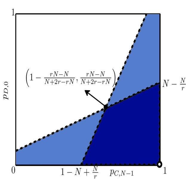
Figure 2: The feasible region of the pinning strategies when $1<r<\frac{N}{N-1}$, which is determined by the intersection of the two half-planes formed in terms of the two linear inequalities in (25), except for the singular point $(p_{C,N-1},p_{D,0})=(1,0)$.

When $1<r<\frac{N}{N-1}$, the conditions $0<p_{C,N-1}^{*}<1$ and $0<p_{D,0}^{*}<1$ are ensured, which means there always exists a feasible region for pinning strategies. The corresponding feasible region is emphasized by dark blue, as shown in Fig. 2. Then, the minimum value of all opponents’ total expected payoff can be reached when $p_{D,0}=0$ and $p_{C,N-1}\neq 1$:

$$\left({\sum\nolimits_{x=2}^{N}{E^{x}}}\right)_{\min}=(N-1).$$ (27)

If $p_{C,N-1}=1$ and $p_{D,0}\neq 0$, the maximum value is:

$$\left({\sum\nolimits_{x=2}^{N}{E^{x}}}\right)_{\max}=r(N-1).$$ (28)

Therefore, the player $1$ can pin his opponents’ average expected payoff to the range between $1$ and $r$ when $r<\frac{N}{{N-1}}$.

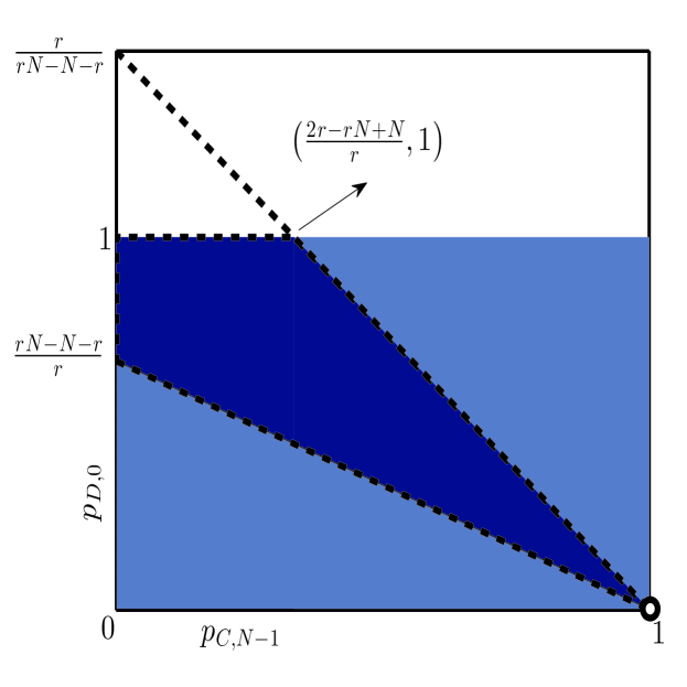
Figure 3: The feasible region of the pinning strategies when $r>\frac{N}{N-1}$, which is determined by the intersection of the two half-planes formed by the two linear inequalities in (30). The intersected region is a convex hull with four extreme points. The region shrinks while the gradients of the two confine lines approaches each other.

Case 2. When $r=\frac{N}{{N-1}}$, the intersecting point reads $(p_{C,N-1}^{*},p_{D,0}^{*})=(0,1)$ and a pinning strategy can be obtained through arbitrarily selecting $p_{C,N-1}$ and $p_{D,0}$ in the region of $[0,1]$ except for the singular point $(p_{C,N-1},p_{D,0})=(1,0)$. Along the line $\gamma p_{D,0}+p_{C,N-1}=1$, the opponents’ total excepted payoff can be pinned into the value determined by Eq. (22), dependent on the parameters $N$, $r$ and $\gamma$. The maximum and minimum values of player $1$’s excepted payoff occurs when all opponents choose always-C and always-D strategies, respectively.

Case 3. When $r>\frac{N}{N-1}$, Eqs. (18) are monotonously decreasing functions of $n$. It is thus sufficient to check the maximum value $p_{C,0}$ and the minimum value $p_{D,N-1}$. Then the probability constrains becomes:

$$p_{C,0} =1+\mu(N-1+r\frac{N-1}{N})+\xi\leq 1,$$ (29a)

$$p_{D,N-1} =\mu r\frac{(N-1)^{2}}{N}+\xi\geq 0.$$ (29b)

Following a similar procedure as Case 1, by substituting Eqs. (20) into Eqs. (29), we can get:

$$rp_{C,N-1}+(rN-N-r)p_{D,0}-r \leq 0,$$ (30a)

$$(rN-N-r)p_{C,N-1}+rp_{D,0}-rN+r+N \geq 0,$$ (30b)

each of which constitutes a closed half-plane in the two-dimensional real space $\mathbb{R}^{2}$. These two half-planes intersect at the dark blue region in Fig. 3, with four extreme points $(0,1)$, $(0,\frac{{rN-N-r}}{r})$, $(\frac{{2r-rN+N}}{{r}},1)$ and $(1,0)$. The feasible region converges to a line $p_{C,N-1}+p_{D,0}=1$ when $\frac{rN-N-r}{r}=\frac{r}{rN-N-r}$, i.e., $r=\frac{N}{N-2}$. The feasible region for the pinning strategies vanishes when $r>\frac{N}{N-2}$. Meanwhile, considering $r>\frac{N}{N-1}$, now we have the two boundaries, as

$$\frac{N}{N-1}<r\leq\frac{N}{N-2}.$$ (31)

According to Eq. (22), we can obtain the minimum and maximum values of the opponents’ total expected payoff in the case of $r>\frac{N}{{N-1}}$:

$$\left({\sum\nolimits_{x=2}^{N}{E^{x}}}\right)_{\min}\left|{{}_{\gamma=\frac{r}{{rN-N-r}}}}\right.=r(N-2+\frac{1}{N}),$$ (32a)

$$\left({\sum\nolimits_{x=2}^{N}{E^{x}}}\right)_{\max}\left|{{}_{\gamma=\frac{{rN-N-r}}{r}}}\right.=(N-1)+r(1-\frac{1}{N}).$$ (32b)

When $r=\frac{N}{N-2}$, $\sum\nolimits_{x=2}^{N}{E^{x}}=\frac{(r+1)^{2}}{2(r-1)}.$

In summary, given the multiplication factor $r$, if player $1$ wants to pin the total expected payoff of all other opponents, it is required that $N\leq\frac{2r}{r-1}$. Or, in a fixed group size $N$, the player $1$ can do this only when $1<r\leq\frac{N}{N-2}$. The upper bound of $r$ as a function of the group size $N$ is presented in Fig. 4. Pinning the total expected payoff of all other opponents is becoming difficult as $N$ grows. Figure 5(a) shows an example 3-player IPGG, where the ZD player $X$ can pin his opponents’ total expected payoff into a fixed value, while his own payoff depends on the opponents’ behaviors: if he would like to set a high value, he may lose more.

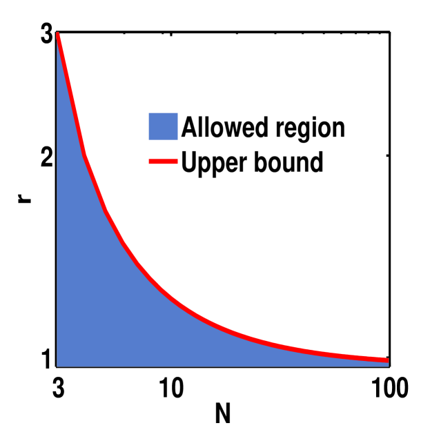
Figure 4: Log-log plot of the upper bound of $r$. The upper bound is a monotonously decreasing function of the group size $N$, namely with the increasing of $N$, the allowed region of multiplication factor for a pinning strategy shrinks.

In the above analysis, one player’s strategy is only conditioned on how many of his opponents cooperate while the detailed information about who cooperate is less important. Such settings may essentially reduce the constrains for the existence of pinning strategies. When considering more complicated scenarios, the constrains necessarily become more strict. For example, there may be more linear inequalities to be satisfied in Eqs. (30) and Eqs. (25). Each inequality constitutes a half-space in the $m$-dimensional real space $\mathbb{R}^{m}$ where $m$ is the number of probability variables in the inequality set. Finding the feasible region of pining strategies is then transferred to the calculation of the intersections of these $m$ half-spaces, which is equivalent to a traditional linear programming problem. Furthermore, since the feasible region for a pining strategy is essentially a convex hull, when analyzing the properties of the pinning strategies, it is sufficient to concentrate on the extreme points. Such feature brings us convenience to further study the game’s equilibriums.

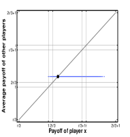
(a)

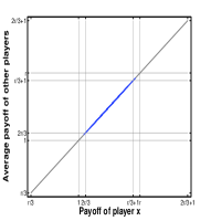
(b)

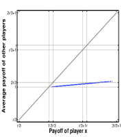
(c)

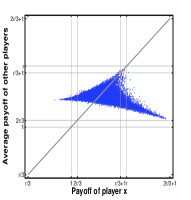
(d)

Figure 5: The payoff of the focal player $X$ against the average payoff of the other two players in an example $3$-player IPGG with $r=1.6$ fixed. (a) The pinning strategy ${\bf{p}}^{X}=[0.08,0.15,0.15,0.22,0.17,0.24,0.24,0.31]^{T}$, corresponding to the state sequence of $CCC$, $CCD$, $CDC$, $CDD$, $DCC$, $DCD$, $DDC$ and $DDD$. (b) The $\chi$-extortion strategy with the minimal $\chi=0.5$ (i.e., $\chi(N-1)=1$) and ${\bf{p}}^{X}=[1.0,0.9,0.9,0.8,0.2,0.1,0.1,0.0]^{T}$, where the ZD player $X$ fairly shares the surplus with his opponents. (c) The $\chi$-extortion strategy with $\chi=7.9$ and ${\bf{p}}^{X}=[0.87,0.87,0.87,0.86,0.01,0,0,0]^{T}$, which is close to the upper bound $\chi=8$. (d) The Win-Stay-Lose-Shift (WSLS) strategy with ${\bf{p}}^{X}=[1,0,0,0,0,1,1,1]^{T}$ for comparison, where the average payoff of the two opponents will distribute a two-dimensional area. Each plot reports the aggregated results from $10^{6}$ independent stage games, where each data point represents the result of one stage game. In each stage game, the strategies of $X$’s two opponents are assigned randomly.

Our analysis indicates that, in an $N$-player IPGG with proper settings, one player can unilaterally control the opponents’ total expected payoff and pin it to a fixed value by playing ZD strategies. In this case, the pinned total expected payoff of opponents is no less than the total endowment of them, which indicates that the player using pinning strategy is nice and may run risk to decrease his own payoff (as indicated by the short horizontal line to the left of the diagonal line in Fig. 5(a)). Generally, in an IPGG, a player can pin the opponents’ total expected payoff when the group size $N$ does not exceed an upper bound, or, when the multiplication factor is not too large. That is to say, the condition for pinning multiple players’ total expected payoff in the IPGG is more strict than pinning a single opponent’s expected payoff in a two-player IPD. In Appendix A, we prove that, in the multi-player IPGG, a ZD player cannot unilaterally set his own expected payoff, analogous to the two-player IPD. In Appendix B, we show that in the multi-player IPGG, two or more players cannot collusively control other players’ payoff.

III.2 Extortion Strategies

Besides pinning the opponents’ total payoff, a ZD player can also extort all his opponents and guarantee that his own surplus over the free-rider’s payoff is $\chi$-fold of the sum of opponents’ surplus. This is the so-called $\chi$-extortion strategy, where $\chi$ is the extortionate ratio. Formally, the extortion strategies for a ZD player $1$ is:

$$\tilde{{\bf{p}}}^{1}=\Phi\left[({\bf{u}}^{1}-\mathbf{1})-\chi\sum_{X=2}^{N}({\bf{u}}^{X}-\mathbf{1})\right].$$ (33a)

Solving this vector equation gives us $2N$ linear equations:

$$p_{C,n}=1+\Phi\left({\frac{{rn}}{N}-\chi\frac{{rn(N-1)-nN}}{N}}\right)$$

$$+\Phi\left({\frac{{r-N}}{N}-\chi\frac{{r(N-1)}}{N}}\right),$$ (34a)

$$p_{D,n}=\Phi\left({\frac{{rn}}{N}-\chi\frac{{rn(N-1)-nN}}{N}}\right),$$ (34b)

for $n\in\{0,1,\cdots,N-1\}$ and $p_{C,n},p_{D,n}\in[0,1]$.

When $\chi\geq 0$, ${\frac{{r-N}}{N}-\chi\frac{{r(N-1)}}{N}}$ is always negative. If $\Phi<0$, the term in the bracket in Eq. (34b) should be non-positive to make $p_{D,n}\geq 0$, leading to $p_{C,n}>1$, which is out of the probability range. The case of $\Phi=0$ corresponds to the singular strategy of $p_{C,n}=1$ and $p_{D,n}=0$ for $n\in\{0,1,...,N-1\}$. Thus it is required that $\Phi>0$. In this case, we have the following linear inequalities as constrains for the extortion strategies:

$$\frac{r(n+1)-N}{N}-\chi\frac{r(n+1)(N-1)-nN}{N}\leq 0,$$ (35a)

$$\frac{rn}{N}-\chi\frac{rn(N-1)-nN}{N}\geq 0.$$ (35b)

Given $n$, $\chi$ is determined by both $r$ and $N$. This is different from the two-player IPD Press2012 where $\chi$ can take any value. From the above two sets of constrains for $\chi$, if $r\leq\frac{N}{N-1}$,

$$\chi\geq\frac{1}{N-1}.$$ (36)

else, if $r>\frac{N}{N-1}$,

$$\frac{1}{N-1}\leq\chi\leq\frac{r}{r(N-1)-N}.$$ (37)

Figures 5(b) and 5(c) show the numerical example of extortion strategies. Within the allowed range of $\chi$ (as shown in the above inequalities), the average payoff of all other opponents falls in a line.

For any value of $r$, $\chi$ has its lower bound. When $r>\frac{N}{N-1}$, $\chi$ also has its upper bound $\frac{r}{r(N-1)-N}$. Normalizing $\sum_{X=2}^{N}({\bf{u}}^{X}-{\bf{1}})$ by the number of opponents $(N-1)$, the ZD player can extort over the average payoff of his opponents by an effective ratio $\chi(N-1)$, which has an upper bound $\frac{r(N-1)}{r(N-1)-N}$. For sufficiently large $N$,

$$\mathop{\lim}_{N\rightarrow\infty}\chi_{\max}(N-1)=\frac{r}{r-1}.$$ (38)

In Fig. 6, we show the value of $\chi_{\max}(N-1)$ as a function of the group size $N$ and the multiplication factor $r$, in the region $r>\frac{N}{N-1}$. As shown in Eq. (38) and Fig. 6, for large $N$, $r$ can be very close to 1, leading to a large maximum effective extortionate ratio $\chi_{\max}(N-1)$. However, under such case, a player is usually not willing to cooperate and thus the payoff in addition to the endowment is tiny. That is to say, although the effective extortionate ratio can be huge, the extorted payoff is not much.

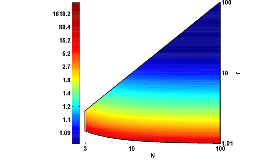
Figure 6: The upper bounds of $\chi(N-1)$ (represented by different colors) versus $N$ and $r$, in the region $r>\frac{N}{N-1}$ and $N\geq 3$.

Substituting the bounds of $\chi$ into the probabilistic strategies in Eqs. (34), we can obtain the allowed range for $\Phi$ as:

$$\Phi\leq\frac{1}{\chi\frac{r(n+1)(N-1)-nN}{N}-\frac{r(n+1)-N}{N}},$$ (39a)

$$0<\Phi\leq\frac{1}{\frac{rn}{N}-\chi\frac{rn(N-1)-nN}{N}}.$$ (39b)

According to the monotonicity, these two inequalities can be reduced to:

$$\begin{split}0<\Phi\leq\frac{N}{N-r+\chi r(N-1)}.\end{split}$$ (40)

Note that $\frac{N}{N-1}$ is monotonously decreasing with $N$. Thus given a specific multiplication factor $r$, the extortionate ratio $\chi$ is more likely to have an upper bound when more players are involved in the game. This means in a game with more players, it will be more difficult for the extortioner to secure his own payoff by using ZD strategy and setting a fixed ratio between his and the opponents’ surplus. A tricky strategy of the extortionate player thus will be restrained when he plays with more opponents. On the other hand, given a fixed group size, a large $r$ will shrink the feasible range of the extortionate ratio. A large multiplication factor $r$ results in a better reward for each player, which promotes mutual cooperations. Therefore, the above analysis reveals the significant fact that, to reduce the possible injuries from a crafty egoist, increasing the cooperation incentive $r$ is an effective approach.

IV Conclusion and Discussions

The discovery of ZD strategies makes us both excited and worried, since a selfish person seems to have a more powerful mathematical tool to extort payoffs from those kindhearted and simpleminded people. Although some recent works Adami2013 ; Hilbe2013 ; Stewart2013 suggested that the extortion strategies in two-player IPD are not evolutionary stable, a few ZD players can still extort other non-ZD opponents in a population. Indeed, compared with those well-known game strategies Axelrod1984 , the ZD strategies are too complicated to be mastered by normal persons, who will eventually become exploitees in the present of ZD players.

To explore the general applicability and limitations of ZD strategies, we have taken a step from two-player games to multi-player games, with the iterated public goods game being the selected template. The bad news learned from our study is that a single ZD player can unilaterally pin the total expected payoff of all other opponents and extort them by enforcing a linear relationship between his own payoff and the opponents’ total payoff. A good news from the results is that the capacity of a ZD player to either pin or extort other opponents is more strictly limited compared with the two-player games. Roughly speaking, we can suppress the influences of the ZD player by increasing the number of participants and/or encouraging cooperation via enlarging the multiplication factor. Taking the global warming problem as an example, if we have made more people being aware of the seriousness of such issue and understanding that the abandonment of some environmentally costly lifestyles is of great significance for the sustainable development, we can to some extent enlarge $N$ and $r$ and thus suppress ZD players. Another good point is that when there are more than one ZD players in the IPGG, they cannot collusively control others but each fights his own battle.

Iterated games with private monitoring represent long-term relationships among players where each player privately receives a noisy (imperfect) observation of the opponents’ actions Nowak1993 . The difficulty of handling such games comes from the fact that players do not share common information under private monitoring, and the decision making in such games involves with complicated statistic inference. Consequently, the analysis, optimization, cooperation enforcement and control in such games have been known as long-standing challenges. This subclass of game theory has found a wide range of applications Mailath2006 , such as evolution in a realistic noisy environment Hansen2004 ; MowakEvo2006 and agent planning under uncertainty Phelan2012 . Whether ZD strategies still works in the noisy environments? Is it still possible for a crafty egoist to control the payoffs of his opponents? These questions ask for future in-depth understanding of ZD strategies.

Both the origin of life and the formation of human societies require cooperation Apicella2012 ; VaidyaNature2012 . During the history of biological evolution, animals and microorganisms such as vampire bats, three-spined sticklebacks, cleaner fishes and bacteria can recognize the importance of reciprocity and even cooperate according to tit-for-tat strategy WilkinsonNature1984 ; MilinskiNature1987 ; BsharyNature2008 ; LeeNature2010 . Male side-blotched lizard and Escherichia coli can play the rock-paper-scissors game in order to maintain biodiversity SinervoNature1996 ; KerrNature2002 . Human is the champion of cooperation. With the growth, children may change from selfishness to egalitarian FehrNature2008 . It is worth exploring whether we can find some field evidences that human beings and animals may be already aware of the existence of ZD strategies during the biological evolution.

Researchers can also design laboratory experiments and study responses of human beings when facing ZD strategies Rand2013 . A player may vary his strategy frequently that cannot generate a Markovian stationary state. Therefore, there are some interesting problems such as whether some proper ZD strategies can control opponents’ payoff in a short timescale and how a smart player alters his ZD strategies in terms of his opponents’ responds. And of course, we firstly want to know whether a normal person will become crazy when facing a crafty ZD player.

Furthermore, for a large population, an individual cannot interact with everybody else. Some individuals usually interact more often than others. The spatial structures of population may affect the maintenance of cooperation. Then some questions natural arise, for example, what is the relationship between the different population structures and related ZD strategies and whether the cooperation can sustain in dynamic social network with the evolution of ZD strategies Santos2011 ; Hauert2002 ; SzaboPRL2002 ; Santos2008 ; RongPRE2010 ; Apicella2012 ; Perc2013 ; RandPNAS2011 . Network analysis is then expected to plays a significant role SzaboFath2007 .

Different from the Prisoner’s Dilemma game which characterizes the pairwise interaction, the public goods game depicts the group interaction. In the pairwise Prisoner’s Dilemma game, only two players take part in one game. If both of them are extortioners, their surpluses become zero that leads to the evolutionary instability of extortion strategies in an infinite population. However, for the public goods game, $N$ players participate in one game. It is difficult to ensure all players are aware of the existence of ZD strategies and use the extortion strategies. Hence, comparing with the pairwise Prisoner’s Dilemma game, the situation for public goods game is more complicated when considering the evolutionary stability. It is relatively easy to analyze the evolutionary stability of ZD versus special strategies, such as always cooperation, always defection, win-stay-lose-shift, and so on. Since the strategy space of public goods game is very huge comparing with Prisoner’s Dilemma game, we should carefully consider how to perform Monte Carlo simulations of population in the framework of weak mutation similar to Ref. Hilbe2013 . Moreover, in this paper we only consider the extortion strategies. Recently good strategies in IPD have been studied Stewart2013 ; Akin2012 , which can to be extended to multi-player IPGG by replacing $\bf{1}$ in Eqs. (33) with $\bf{r}$. Then the robustness of good and generosity strategies can be deeply analyzed in the next step. In addition, the evolutionary stability analysis of IPGG can also be combined with the studies on the effects of reward and punishment SigmundPNAS01 ; Sigmund2010 ; Sasaki2012 .

Appendix A $X$ tries to set his own payoff

A ZD player $X$ cannot unilaterally set his own payoff in the PD, here we obtain the same conclusion for iterated PGG. If he tries to set his own payoff, he must choose $\tilde{p}^{X}=\alpha_{1}S_{1}+\alpha_{0}\mathbf{1}$. The linear equations now become

$$p_{C,n}=1+\alpha_{1}\frac{r(n+1)}{N}+\alpha_{0},$$ (41)

$$p_{D,n}=\alpha_{1}\frac{rn+N}{N}+\alpha_{0}.$$ (42)

Setting $p_{C,N-1}$ and $p_{D,0}$ as free variables, we have

$$\alpha_{1} =\frac{p_{C,N-1}-p_{D,0}-1}{r-1}.$$ (43a)

$$\alpha_{0} =\frac{rp_{D,0}-p_{C,N-1}+1}{r-1}.$$ (43b)

Since $p_{C,n},p_{D,n}$ are decreasing functions of $n$, we have

$$p_{C,N-2} =1+\alpha_{1}\frac{r(N-1)}{N}+\alpha_{0}\geq 0$$ (44a)

$$p_{C,0} =1+\alpha_{1}\frac{r}{N}+\alpha_{0}\leq 1$$ (44b)

$$p_{D,N-1} =\alpha_{1}\frac{r(N-1)+N}{N}+\alpha_{0}\geq 0$$ (44c)

$$p_{D,1} =\alpha_{1}\frac{r+N}{N}+\alpha_{0}\leq 1.$$ (44d)

After some algebra, (44b) can be reduced to

$$p_{D,0}\leq\frac{(N-r)p_{C,N-1}-(N-r)}{rN-r}.$$ (45)

Since $r\leq N$ for PGG, this leads to $p_{D,0}\leq 0$. So a ZD player $X$ cannot set his own payoff.

Appendix B Collusive strategies

In the determinant form of player’s payoff, there are columns which are controlled by more than one players. This suggests that there might be collusive strategies, which means more than one players trying to control other players’ payoff collusively. However this type of ZD strategies generally does not exit. Take the $two-$player collusive strategies as an example. Denote the column controlled tangly by the player $X$ and $Y$ by $\tilde{pq}$. For general ZD strategies $\tilde{pq}=\sum_{X=1}^{N}\alpha_{X}{\bf S}_{X}+\alpha_{0}\mathbf{1}$, the following $2N$ linear equations must be satisfied: $p_{C,n}q_{C,n}=1+\Theta_{1}$, $p_{D,n}q_{D,n}=\Theta_{2}$, $p_{C,n}q_{D,n}=\Theta_{3}$, and $p_{D,n}q_{C,n}=\Theta_{4}$. Here $\Theta_{1}$,$\Theta_{2}$,$\Theta_{3}$ and $\Theta_{4}$ depend on the specific values of $\alpha_{k}$ and $\alpha_{0}$. From the above constrains, we obtain

$$\frac{p_{C,n}q_{C,n}}{p_{D,n}q_{C,n}}=\frac{p_{C,n}q_{D,n}}{p_{D,n}q_{D,n}}.$$ (46)

This is a very strong constraint, and generally cannot be satisfied.

References

- (1) R. Axelrod and W. D. Hamilton, Science 211, 1390 (1981).
- (2) R. Axelrod, The Evolution of Cooperation (New York: Basic Book, 1984).
- (3) R. Axelrod and D. Dion, Science 242, 1385 (1988).
- (4) M. A. Nowak and K. Sigmund, Nature 364, 56 (1993).
- (5) M. A. Nowak, Science 314, 1560 (2006).
- (6) G. Kendall, X. Yao, and S. Y. Chong, The Iterative Prisoners’ Dilemma: 20 Years On (Singapore, World Scientific, 2007).
- (7) W. H. Press and F. J. Dyson, Proc. Acad. Natl. Sci. U.S.A. 109, 10409 (2012).
- (8) C. Adami and A. Hintze, Nature Commun. 4, 3193 (2013).
- (9) C. Hilbe, M. A. Nowak, and K. Sigmund, Proc. Acad. Natl. Sci. U.S.A. 110, 6913 (2013).
- (10) A. J. Stewart and J. B Plotkin, Proc. Acad. Natl. Sci. U.S.A. 110, 15348 (2013).
- (11) E. Akin, arXiv:1211.0969 (2012).
- (12) J. Chen and A. Zinger (unpublished).
- (13) C. Hilbe, M. A. Nowak, and A. Traulsen, PLoS ONE 8, e77886 (2013).
- (14) A. A. Daoud, G. Kesidis, and J. Liebeherr, arXiv: 1401.3373 (2014).
- (15) A. Szolnoki and M. Perc, arXiv: 1401.8294 (2014).
- (16) A. J. Stewart and J. B. Plotkin, Proc. Acad. Natl. Sci. U.S.A. 109, 10134 (2012).
- (17) B. Hayes, American Scientist 101, 422 (2013).
- (18) L. Roemheld, arXiv: 1308.2576.
- (19) G. Hardin, Science 162, 1243 (1968).
- (20) J. H. Kagel and A. E. Roth, The Handbook of Experimental Economics (Princeton University Press, Princeton, 1995).
- (21) E. Fehr and U. Fischbacher, Nature 425, 785 (2003).
- (22) O. X. Cordero, L.-A. Ventouras, E. F. DeLong, and M. F. Polz, Proc. Acad. Natl. Sci. U.S.A. 109, 20059 (2012).
- (23) H. Bachmann, M. Fischlechner, I. Rabbers, N. Barfa, F. B. dos Santos, D. Molenaar, and B. Teusink, Proc. Acad. Natl. Sci. U.S.A. 110, 14302 (2013).
- (24) M. Milinski, D. Semmann, H. J. Krambeck, and J. Marotzke, Proc. Acad. Natl. Sci. U.S.A. 103, 3994 (2006).
- (25) M. Milinski, R. D. Sommerfeld, H. J. Krambeck, F. A. Reed, and J. Marotzke, Proc. Acad. Natl. Sci. U.S.A. 105, 2291 (2008).
- (26) A. Tavonia, A. Dannenberg, G. Kallis, and A. Löschel, Proc. Acad. Natl. Sci. U.S.A. 108, 11825 (2011).
- (27) F. C. Santos and J. M. Pacheco, Proc. Acad. Natl. Sci. U.S.A. 108, 10421 (2011).
- (28) K. Sigmund, C. Hauert, and M. A. Nowak, Proc. Natl. Acad. Sci. U.S.A. 98, 10757(2001).
- (29) C. Hauert, S. De Monte, J. Hofbauer, and K. Sigmund, Science 296, 1129 (2002).
- (30) G. Szabó and C. Hauert, Phys. Rev. Lett. 89, 118101 (2002).
- (31) F. C. Santos, M. D. Santos, and J. M. Pacheco, Nature 454, 213 (2008).
- (32) Z. Rong, H.-X. Yang, and W.-X. Wang, Phys. Rev. E 82, 047101 (2010).
- (33) C. L. Apicella, F. W. Marlowe, J. H. Fowler, and N. A. Christakis, Nature 481, 497 (2012).
- (34) M. Perc, J. Gómez-Gardeñes, A. Szolnoki, L. M. Floría, and Y. Moreno, J. R. Soc. Interface 10, 20120997 (2013).
- (35) E. Fehr and S. Gächter, Am. Econo. Rev. 90, 980 (2000).
- (36) M. Milinski, D. Semmann, and H. J. Krambeck, Nature 415, 424 (2002).
- (37) D. F. Zheng, H. P. Yin, C. H. Chan, and P. M. Hui, Europhys. Lett. 80, 18002 (2007).
- (38) J. M. Pacheco, F. C. Santos, M. O. Souza, and B. Skyrms, Proc. R. Soc. Lond. B 276, 315 (2009).
- (39) G. Mailath and L. Samuelson, Repeated Games and Reputation (Oxford University Press, 2006).
- (40) E. A. Hansen, D. S. Bernstein, and S. Zilberstein, In: Proceedings of the Nineteenth National Conference on Artificial Intelligence (AAAI-04), pages 709-715, AAAI Press, 2004.
- (41) M. Nowak, Evolutionary Dynamics: Ex-ploring the Equations of Life (Harvard University Press, 2006).
- (42) C. Phelan and A. Skrzypacz, Review of Economic Studies 79 1637 (2012).
- (43) N. Vaidya, M. L. Michael, I. A. Chen, R. Xulvi-Brunet, E. J. Hayden, and N. Lehman, Nature 491, 72 (2012).
- (44) G. S. Wilkinson, Nature 308, 181 (1984).
- (45) M. Milinski, Nature 325, 433 (1987).
- (46) R. Bshary, A. S. Grutter, A. S. T. Willener, and O. Leimar, Nature 455, 964 (2008).
- (47) H. H. Lee, M. N. Molla, C. R. Cantor, and J. J. Collins, Nature 467, 82 (2010).
- (48) B. Sinervo and C. M. Lively, Nature, 380, 240 (1996).
- (49) B. Kerr, M. A. Riley, M. W. Feldman, and B. J. M. Bohannan, Nature 418, 171 (2002).
- (50) E. Fehr, H. Bernhard, and B. Rockenbach, Nature 454, 1079 (2008).
- (51) D. G. Rand and M. A. Nowak, Trends Cogn. Sci. 17, 413 (2013).
- (52) D. G. Rand, S. Arbesman, N. A. Christakis, Proc. Natl. Acad. Sci. U.S.A. 108, 19193 (2011).
- (53) G. Szabó and G. Fath, Phys. Rep. 446, 97 (2007).
- (54) K. Sigmund, H. D. Silva, A. Traulsen, and C. Hauert, Nature 466, 816 (2010).
- (55) T.Sasaki, Å. Brännströma, U. Dieckmann, and K. Sigmund, Proc. Natl. Acad. Sci. U.S.A. 109, 1165(2012).