A search for H I absorption in nearby radio galaxies using HIPASS

Abstract

Using archival data from the H i Parkes All Sky Survey (HIPASS) we have searched for 21 cm line absorption in 204 nearby radio and star-forming galaxies with continuum flux densities greater than $S_{1.4}\approx 250$ mJy within the redshift range $0<cz<12\,000\,\mathrm{km}\,\mathrm{s}^{-1}$. By applying a detection method based on Bayesian model comparison, we successfully detect and model absorption against the radio-loud nuclei of four galaxies, of which the Seyfert 2 galaxy 2MASX J130804201-2422581 was previously unknown. All four detections were achieved against compact radio sources, which include three active galactic nuclei (AGNs) and a nuclear starburst, exhibiting high dust and molecular gas content. Our results are consistent with the detection rate achieved by the recent ALFALFA (Arecibo Legacy Fast Arecibo L-band Feed Array) H i absorption pilot survey by Darling et al. and we predict that the full ALFALFA survey should yield more than three to four times as many detections as we have achieved here. Furthermore, we predict that future all-sky surveys on the Square Kilometre Array precursor telescopes will be able to detect such strong absorption systems associated with type 2 AGNs at much higher redshifts, providing potential targets for detection of H₂O megamaser emission at cosmological redshifts.

1 Introduction

Atomic hydrogen (H i) gas, traced by the 21 cm line, is a powerful probe of the mass distribution within galaxies and the available fuel for future star formation. However, the strength of the 21 cm emission-line decreases rapidly with increasing redshift as a function of the inverse square of the luminosity distance. In individual galaxies the most distant detectable 21 cm emission lines are at $z\sim 0.2$ (e.g. Catinella et al., 2008; Verheijen et al., 2010; Freudling et al., 2011), while statistical detections using spectral stacking have reached $z\approx 0.37$ (Lah et al., 2009). At significantly higher redshifts, we can instead detect the 21 cm line in individual galaxies through the absorption of continuum flux towards a background radio source. In principle, H i absorption can be observed up to cosmological redshifts, where the ionosphere begins to corrupt the signal, yet such observations are ultimately limited by the sample of known high-redshift radio sources and the availability of suitable instrumentation. The highest redshifts achieved by observations of 21 cm absorbers include the radio galaxy B2 0902+34 ($z=3.397$; Uson et al. 1991) and the intervening system towards the quasar PKS 0201+113 ($z=3.387$; Kanekar et al. 2007). The detection limit for a survey of 21 cm line absorption is independent of redshift, and depends only on the availability of bright background continuum sources against which the line can be detected. For any such sight line, absorption is particularly sensitive to high column densities ($N_{\mathrm{HI}}\gtrsim 10^{20}\,\mathrm{cm}^{-2}$) of cold ($T_{\mathrm{spin}}\lesssim 100$ K) foreground H i gas that obscures a large fraction of the background radio source.

In the local Universe, at least 10  per cent of extragalactic radio sources that have been searched exhibit an associated 21 cm absorption line at or near the optical redshift, indicating that neutral gas is present within the host galaxy (e.g. Morganti et al., 2001; Vermeulen et al., 2003; Allison et al., 2012a). High signal-to-noise ratio (S/N) absorption lines, typically associated with powerful radio galaxies, often exhibit broad wings, which can indicate the presence of fast jet-driven outflows of H i gas (with velocities over 1000 km s^-1 and outflow rates of several tens of M_⊙ yr^-1; e.g. Morganti et al. 2005; Mahony et al. 2013; Morganti et al. 2013). These high-velocity outflows may have a profound effect on the star formation and subsequent evolution of the host galaxy. Furthermore, there is evidence to suggest that in some cases broad absorption components can arise in circumnuclear gas distributed as a disc or torus (e.g. Struve & Conway, 2010; Morganti et al., 2011). Such observations are incredibly useful for directly studying the interaction between the radio-loud nucleus and the neutral gas in the interstellar medium. However, at present these surveys are limited to targeted sampling of the radio source population, typically focusing on those that are compact, and by doing so can introduce biases (see e.g. Curran & Whiting, 2010).

Here we present the results of a search for 21 cm absorption in nearby radio and star-forming galaxies from the H i Parkes All-Sky Survey (HIPASS; Barnes et al. 2001). While the data are considerably less sensitive than current targeted observations of radio sources (with an effective integration time of 7.5 min per individual pointing and typical rms noise of $\sim$13 mJy beam^-1 per 13 km s^-1 channel separation), the large volume covered by HIPASS (the whole sky south of $\delta=+25^{\circ}$ and $z\lesssim 0.042$) allows identification of the strongest associated H i absorption-line systems in the local universe in an unbiased way. This enables us to study some of the most extreme and potentially interesting systems, as well as testing line-finding techniques (e.g. Allison et al., 2012b) that can be used in planning future, more sensitive, large-area surveys with the Square Kilometre Array (SKA) pathfinder and precursor telescopes.

Darling et al. (2011) recently published the results of a pilot survey for H i 21 cm absorption in the Arecibo Legacy Fast Arecibo L-band Feed Array (ALFALFA) survey. This was the first genuinely blind search for absorption within a large-area radio survey, and covered 517 deg² of sky in the redshift range $z<0.058$. No intervening lines were seen, but one previously known associated line was re-detected in the interacting luminous infrared galaxy UGC 6081 (Bothun & Schommer, 1983; Williams & Brown, 1983). The HIPASS search presented here can be considered complementary to that survey, since it covers a much larger area of sky (by approximately a factor of 50) with similar redshift coverage, but has lower sensitivity (by approximately a factor of 6). However, due to the presence of strong baseline ripple, we have limited our search to the detection of H i absorption within the host galaxies of the radio sources themselves. Spectral baseline ripples are a common problem for single-dish observations of the 21 cm line (e.g. Briggs et al., 1997) and HIPASS spectra towards bright continuum sources are particularly affected, where standing waves are generated between the primary dish and receiver cabin (Barnes et al., 2001, 2005). By using the known systemic redshift of the galaxy as a prior, we can attempt to distinguish the absorption-line from the strong baseline ripple. We intend in future work to revisit the HIPASS data with improved analysis and perform an extended search of intervening H i absorption within the full volume.

Throughout this paper we adopt a flat $\Lambda$ cold dark matter cosmology with $H_{0}$ = 70 km s^-1, $\Omega_{\mathrm{M}}$ = 0.3 and $\Omega_{\Lambda}$ = 0.7. Radial velocities and redshifts have been corrected for the solar barycentric standard-of-rest frame.

2 Sample selection

Our sample selection was driven by the brightest radio sources in the National Radio Astronomy Observatory Very Large Array Sky Survey (NVSS, $\nu=1.4$ GHz; Condon et al., 1998), the Sydney University Molonglo SkySurvey (SUMSS, $\nu=843$ MHz; Mauch et al., 2003) and the second epoch Molonglo Galactic Plane Survey (MGPS-2, $\nu=843$ MHz; Murphy et al., 2007). Together, the footprints of these three surveys fully overlap the sky coverage of HIPASS down to continuum flux densities of a few mJy. The typical noise per median-gridded HIPASS image is $\sim$ 13 mJy beam^-1 (with spectral channels separated by 13.2 km s^-1 at z = 0) but can vary significantly as a function of system temperature and the number of gridded pointings contributing to the image. By considering those radio sources that have integrated flux densities above 250 mJy (at either 843 MHz or 1.4 GHz), which would enable us to detect absorption lines with peak optical depths greater than 30 per cent against the weakest sources, we have constructed a sample of 19 237 within the HIPASS footprint of $-90\degr<\delta<+25\degr$. To obtain a sample of nearby radio and star-forming galaxies, we simply matched this list of radio sources with their optical counterparts and selected those that have redshifts within the HIPASS volume. However, to significantly improve the completeness of our sample we also considered the catalogue of van Velzen et al. (2012), who have used a more sophisticated method to match radio sources with their counterparts in the Two Micron All-Sky Survey (2MASS Skrutskie et al., 2006) Redshift Survey (Huchra et al., 2012).

2.1 Sample 1: radio–optical matches

In the first instance, we construct a sample of nearby radio and star-forming galaxies that have known redshifts in the range $cz<12\,000$ km s^-1, by matching our catalogue of 19 237 radio sources with their optical counterparts using the MultiCone search function of the TopCat software package (Taylor, 2005). The optical counterparts were selected using catalogues from the 6dF Galaxy Survey (6dF GS; Jones et al., 2009) and the CfA Redshift Survey (Huchra et al. 1999 and references therein), or otherwise from the NASA Extragalactic Database. Based on the work of Mauch & Sadler (2007), who matched radio sources in NVSS with galaxies in 6dF GS (for $0.003<z<0.3$), we assume that a maximum displacement of 10 arcsec is sufficient to produce a reliable identification of a radio-optical source pair. Of these radio-optical pairs, we identified 105 with optical spectroscopic redshifts in the range spanned by the HIPASS data. A further 15 matches were then excluded from the sample, in most cases due to unreliable redshift measurements (see Appendix A), resulting in a final list of 90 nearby galaxies that form our first sample.

2.2 Sample 2: the van Velzen et al. sample

The recently compiled catalogue of nearby radio and star-forming galaxies by van Velzen et al. (2012) was constructed by matching radio sources in the NVSS and SUMSS catalogues with their optical counterparts in the 2MASS Redshift Survey (2MRS; Huchra et al. 2012), covering 88 per cent of the sky at redshifts of $z\lesssim 0.052$. This catalogue consists of 575 galaxies with apparent $K_{s}$-band magnitudes brighter than 11.75 and total flux densities above limits of 213 mJy at 1.4 GHz and 289 mJy at 843 MHz. Importantly, matches were made between multiple radio components and a single galaxy, thereby providing reliable estimates of the total radio flux density in extended emission. Given that the MGPS-2 catalogue only identifies compact radio components, van Velzen et al. did not consider these galactic-plane sources and so any sample constructed from their catalogue will not contain sources with Galactic latitude $|b|<10\degr$ south of $\delta=-30\degr$. From this parent catalogue, we have selected a second sample of 189 galaxies that are bounded by the volume $cz<12\,000$ km s^-1 and $-90\degr<\delta<+25\degr$.

2.3 Properties of our sample

By comparing the content of our two samples, we found that 75 of the galaxies in Sample 1 are common to those in Sample 2, while the remaining 15 either have radio flux densities or 2MASS $K_{s}$-band magnitudes below the limits imposed by van Velzen et al. (2012), or are in the MGPS-2 compact source catalogue. Therefore, our total sample contains 204 unique radio-detected galaxies. van Velzen et al. defined morphological classifications for their radio galaxy sample based on the extent and distribution of the radio emission compared with the near-infrared emission. By applying those same classifications to our sample, we find that 39 are point sources, 124 are jets and lobes, 36 are star-forming galaxies and 5 are unknown. Those galaxies that have an unknown classification are potentially the result of a random match with a background radio source; however, we have decided to include these in our sample since they still provide reasonable candidates for H i absorption.

The completeness of our combined sample will be limited by that of the parent catalogues (for example the MGPS-2 compact source catalogue of the galactic plane excludes the 10 per cent of extended radio sources predicted by SUMSS), and the matching algorithms employed (for example our 10 arcsec position-matching criterion for Sample 1 will exclude some nearby large radio and star-forming galaxies). To provide an estimate of the completeness, we compare the total number of radio and star-forming galaxies in our sample with that predicted from the local luminosity function at 1.4 GHz. The HIPASS footprint covers an area of sky equal to 29 343 deg² (Meyer et al., 2004; Wong et al., 2006), and so with an upper redshift limit of $cz<12\,000$ km s^-1 our sample spans a comoving volume of 0.0146 Gpc³. Based on the local radio luminosity function given by Mauch & Sadler (2007), which was measured from a sample of 6667 galaxies at $0.003<z<0.3$, we predict that there are approximately 230 galaxies within the HIPASS volume above a flux density limit of 250 mJy and 260 above 213 mJy. Our sample of 204 galaxies therefore represents an approximately 80–90 per cent complete flux-limited list of nearby radio and star-forming galaxies in the HIPASS footprint, not accounting for the uncertainties generated by counting statistics, cosmic variance and the effects of galaxy clustering. We list in Appendix B the properties of candidates that form our sample, and in Fig. 1 we show their distribution as a function of redshift.

3 H I absorption in HIPASS

3.1 Spectra extraction

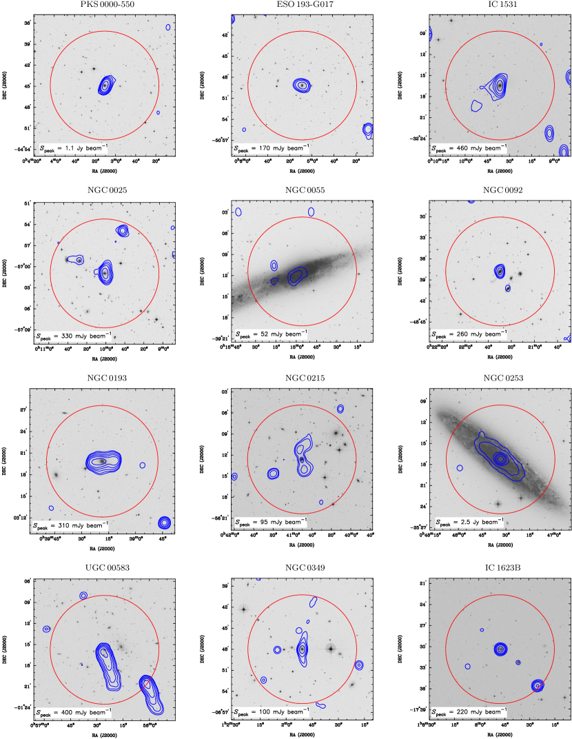
Figure 15: Images of 204 galaxies searched for H i absorption using HIPASS. The blue contours denote the 1, 2, 5, 10, 20, 50 per cent levels of the peak radio flux density within the HIPASS beamwidth, from either NVSS ($\delta>-30\degr$, $\nu=1.4$ GHz, typical beam FWHM = 45 arcsec) or SUMSS/MGPS-2 ($\delta<-30\degr$, $\nu=843$ MHz, typical beam FWHM = 45 arcsec). For clarity, we exclude those radio contours that are less than five times the survey rms. The large red circle represents the gridded HIPASS beamwidth of 15.5 arcmin. The grey-scale images represent optical $B_{j}$-band photometry from the SuperCosmos Sky Survey, using the UK Schmidt and Palomar Oschin Schmidt telescopes (Hambly et al., 2001). The full version of this figure is available online.

Calibration and imaging of the Parkes 21 cm multibeam data was described in extensive detail by Barnes et al. (2001), with further descriptions of the final HIPASS emission-line catalogues by Koribalski et al. (2004), Meyer et al. (2004) and Wong et al. (2006). For each galaxy in our two samples, we have searched for H i absorption in a single integrated spectrum towards the centroid position of the radio source. The spectra were extracted from the data cubes by implementing the task Mbspect in the Multichannel Image Reconstruction, Image Analysis and Display package (Miriad; Sault et al. 1995). The gridded beamwidth of each HIPASS image is 15.5 arcmin, and so we assume that any H i absorption in the target galaxy will be detected in a single pencil beam towards the spatially unresolved radio emission. The overlaid radio contours and optical images shown in Fig. 15 for our sample show that this assumption is valid.

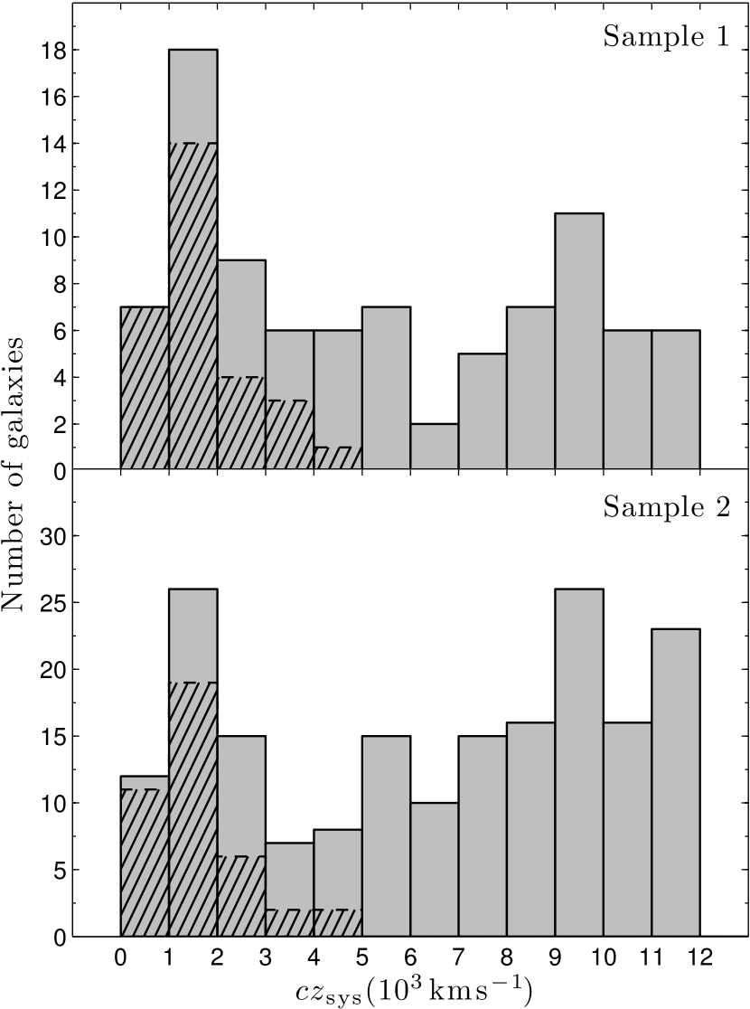
Figure 1: The distribution of systemic redshifts for our two samples of galaxies. The hatched bars represent those with catalogued 21 cm line emission in HIPASS (Koribalski et al. 2004; Meyer et al. 2004; Wong et al. 2006), dominating at redshifts less than $cz_{\mathrm{sys}}=5000$ km s^-1.

The flux density spectrum of each unresolved radio source is calculated by taking the following weighted sum over a square region of nine by nine 4 arcmin pixels, as follows

$$S(\nu)=\sum_{i}{w_{i}^{\prime}}S_{i}(\nu),$$ (1)

and

$$w_{i}^{\prime}={w_{i}\over\sum_{i}{{w_{i}}^{2}}},$$ (2)

where $S_{i}(\nu)$ and $w_{i}$ are the flux density and weighting, respectively, for the $i$th pixel. For an elliptical beam, with position angle $\phi$ and axes with full width at half maxima (FWHMs) of $\theta_{\mathrm{maj}}$ and $\theta_{\mathrm{min}}$, the beam weights are given by

$$w_{i}=\exp{\left[-2\ln{(4)}(A_{i}+B_{i}+C_{i})\right]},$$ (3)

where

$$A_{i} = [(\sin{(\phi)}/\theta_{\mathrm{maj}})^{2}+(\cos{(\phi)}/\theta_{\mathrm{min}})^{2}]~{}(\Delta{\alpha_{i}})^{2},$$

$$B_{i} = \sin{(2\phi)}~{}[(1/\theta_{\mathrm{maj}})^{2}-(1/\theta_{\mathrm{min}})^{2}]~{}\Delta{\alpha_{i}}~{}\Delta{\delta_{i}},$$

$$C_{i} = [(\cos{(\phi)}/\theta_{\mathrm{maj}})^{2}+(\sin{(\phi)}/\theta_{\mathrm{min}})^{2}]~{}(\Delta{\delta_{i}})^{2},$$ (4)

and $\Delta{\alpha_{i}}$ and $\Delta{\delta_{i}}$ are the angular distances from the centre position, in right ascension and declination, respectively. For the median-gridded HIPASS images, $\phi=0\degr$ and $\theta_{\mathrm{maj}}=\theta_{\mathrm{min}}=15.5$ arcmin, so in this case the beam weighting parameters are given by

$$A_{i,\mathrm{HIPASS}} = (\Delta{\alpha_{i}}/15.5\mathrm{\,arcmin})^{2},$$

$$B_{i,\mathrm{HIPASS}} = 0,$$

$$C_{i,\mathrm{HIPASS}} = (\Delta{\delta_{i}}/15.5\mathrm{\,arcmin})^{2}.$$ (5)

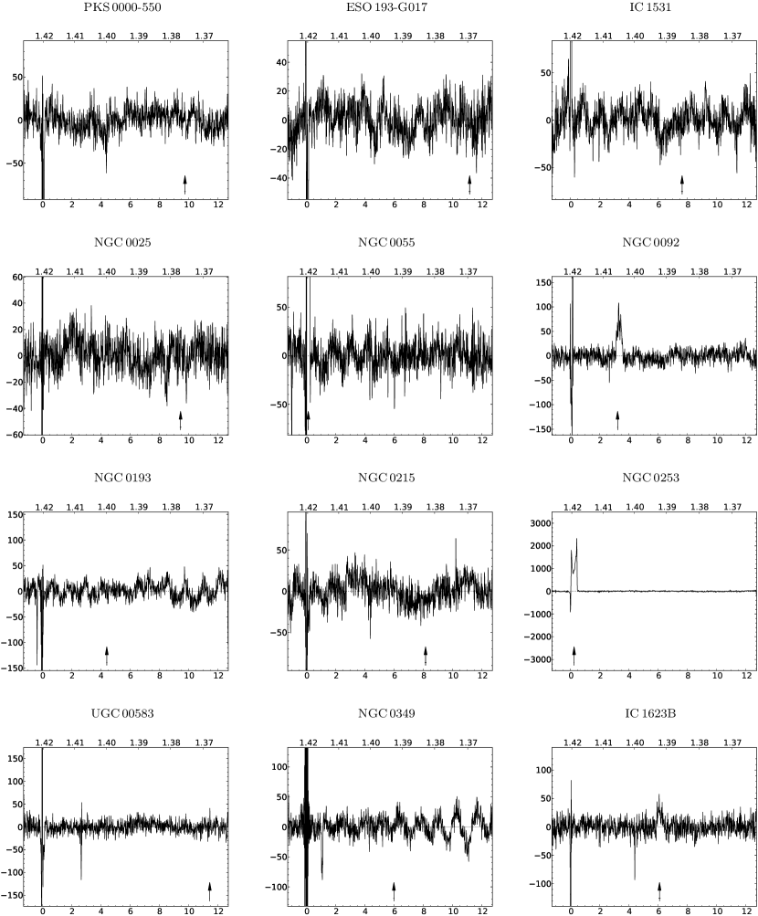
Figure 16: HIPASS spectra of 204 galaxies searched for H i absorption. For each spectrum, the ordinate shows the beam-weighted flux density (in mJy), the lower abscissa the Doppler corrected barycentric redshift (in 1000 km s^-1) and the upper abscissa the observed frequency (in GHz). The arrow and horizontal line indicate the mean and uncertainty in the systemic redshift of the galaxy. The full version of this figure is available online.

The extracted HIPASS spectra for each of our 204 galaxies are shown in Fig. 16.

3.2 Noise estimation

In order to estimate the significance of individual spectral components of a given HIPASS spectrum, we must characterize the properties of the noise. The archival HIPASS data cubes were constructed by gridding together individual spectra using a median estimator to the beam-weighted average (Barnes et al., 2001). The median of a randomly distributed variable is asymptotically normal, and so given that the noise in the individual ungridded spectra is approximately normal and that the beam weights are randomly distributed on the sky, we assume that the noise in the median-gridded spectra is also normal. In a given data cube, we allow for spectral variation in the noise by calculating the median absolute deviation from the median (MADFM) across each image plane. The MADFM per pixel ($s_{\rm pixel}$) is given by

$$s_{\rm pixel}=\mathrm{med}(|d_{i}-\mathrm{med}(d_{i})|),$$ (6)

where $d_{i}$ is the value of the $i$th pixel in the image. The standard deviation per pixel ($\sigma_{\rm pixel}$), assuming that the pixel noise is normally distributed, can then be estimated by (Whiting 2012)

$$\sigma_{\rm pixel}=[\sqrt{2}\mathrm{erf}^{-1}(0.5)]^{-1}\,s_{\rm pixel}\approx 1.483\,s_{\rm pixel},$$ (7)

where $\mathrm{erf}^{-1}$ is the inverse of the Gauss error function. Fig. 2 shows the distribution of the estimated pixel noise per channel per sight-line for our sample of galaxies, peaking in the range 13–14 mJy beam^-1. This method provides a robust estimator of the pixel noise for a given channel, but does not account for spatial variation across the data cube. Furthermore, the MADFM is a robust estimator of the noise for data where sources occupy a relatively small number of pixels with respect to the total size of the image, yet it may become a poor estimator in channels containing extended strong signal, such as that from the 21 cm line in the Milky Way.

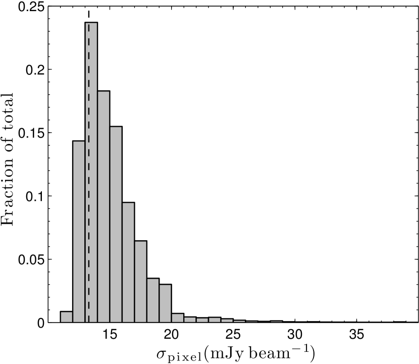
Figure 2: The distribution of pixel noise (standard deviation) per HIPASS channel per sight-line for our sample of 204 galaxies, estimated using the MADFM over each image plane of each data cube. For comparison we show the canonical rms noise (vertical dashed line) for the HIPASS southern data (13.3 mJy beam^-1; Barnes et al. 2001).

The standard deviation ($\sigma_{\rm S}$) in the flux density ($S$) defined by Equation 1 is given by

$$\sigma_{\rm S}^{2}=\mn@boldsymbol{w}^{\rm t}\,\textbf{{C}}_{\rm pixel}\,\mn@boldsymbol{w},$$ (8)

where $\mn@boldsymbol{w}$ is the vector of weights ($w_{\rm i}^{\prime}$) defined by Equation 2 and $\textbf{{C}}_{\rm pixel}$ is the image pixel covariance matrix. If we assume that the per-pixel noise has a single value ($\sigma_{\rm pixel}$), we can simplify this expression to

$$\sigma_{\rm S}^{2}=(\mn@boldsymbol{w}^{\rm t}\,\textbf{{R}}_{\rm pixel}\,\mn@boldsymbol{w})\,\sigma_{\rm pixel}^{2},$$ (9)

where $\textbf{{R}}_{\rm pixel}$ is the pixel correlation matrix. The noise correlation between pixels is generated by a combination of the intrinsic properties of the telescope (such as the beam) and the gridding procedure implemented by Barnes et al. Rather than analytically modelling this relationship between $\sigma_{\rm S}$ and $\sigma_{\rm pixel}$, which would require knowledge of the relative contributions of these factors, we estimate it empirically by generating multiple Monte Carlo realizations of the flux density $S$ per image per data cube. Following this empirical procedure, we find that

$$\sigma_{\rm S}\approx(0.95\pm 0.10)\,\sigma_{\rm pixel},$$ (10)

and so apply a correction factor of 0.95 to the pixel noise when estimating the noise level in our extracted spectra.

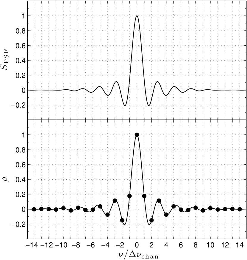
Figure 3: Top: the spectral response of HIPASS to an unresolved positive signal centred at channel 0 and normalized to unity. Bottom: the resulting correlation function ($\rho$) given by Equation 11. The circles represent the correlation coefficients sampled at the channel separation $\Delta{\nu_{\mathrm{chan}}}$.

3.3 Covariance estimation

A common consideration for lag correlators, such as that used for HIPASS, is the effect of a strong signal in the unfiltered time-lag spectrum, which introduces severe Gibbs ringing in the frequency domain. To significantly reduce this effect, Barnes et al. applied a 25 per cent Tukey filter to the time-lag data, diminishing the spectral resolution by 15 per cent and effectively increasing the FWHM of the spectral point spread function to approximately 18 km s^-1. Using this information, we can model the correlation ($\rho$) as a function of frequency ($\nu$) by taking the autocorrelation of the known spectral point spread function ($S_{\mathrm{PSF}}$, top panel of Fig. 3), which in algebraic form is given by

$$\rho(\nu)=\rho_{0}^{-1}\int_{-\infty}^{\infty}{S_{\mathrm{PSF}}(\nu^{\prime})S_{\mathrm{PSF}}(\nu+\nu^{\prime})}\mathrm{d}\nu^{\prime},$$ (11)

where

$$\rho_{0}=\int_{-\infty}^{\infty}{S_{\mathrm{PSF}}(\nu^{\prime})}^{2}\mathrm{d}\nu^{\prime}.$$ (12)

The correlation coefficients between discrete HIPASS spectral channels can then be calculated by sampling $\rho(\nu)$ at integer channel separations (see the bottom panel of Fig. 3). Using these correlation coefficients we can estimate the noise covariance ($\sigma_{ij}^{2}$) between the $i$th and $j$th channels by

$$\sigma_{ij}^{2}=\rho_{ij}\,\sigma_{i}\,\sigma_{j},$$ (13)

where $\rho_{ij}$ is the correlation coefficient and $\sigma_{i}$ is an estimate of the standard deviation due to the noise in channel $i$. These covariances form the off-diagonal elements of the matrix C, while the per-channel variances ($\sigma_{i}^{2}$) form the diagonal. We note that it is also possible, with enough information, to model other components of the covariance. For example, we could account for the aforementioned standing waves that dominate single-dish spectra towards radio continuum sources or, in the case of interferometers, the spectral ripple that can arise as a result of imaging a field of continuum sources with incomplete sampling of the Fourier plane. While this will be pursued in future work, here we choose to consider the effects of these systematics a posteriori, and therefore compare our spectral models based purely on their significance above our estimate of the correlated noise.

3.4 Automated line finding and parametrization

We automatically detect and parametrize the H i absorption by using a Bayesian approach to model comparison, the application of which was described by Allison et al. (2012a, b). This method determines the significance of a detection above the noise by comparing the posterior probability of the absorption-line and continuum model ($\mathcal{M}_{\mathrm{HI}}$) with that of the continuum-only model ($\mathcal{M}_{\mathrm{cont}}$), given the data. Using Bayes’ theorem, the posterior probabilities of the two models are related to the marginal likelihoods (also known as the evidence), $\mathrm{Pr}(\mn@boldsymbol{d}|\mathcal{M})$, and priors, $\mathrm{Pr}(\mathcal{M})$, by

$${\mathrm{Pr}(\mathcal{M}_{\mathrm{HI}}|\mn@boldsymbol{d})\over\mathrm{Pr}(\mathcal{M}_{\mathrm{cont}}|\mn@boldsymbol{d})}={\mathrm{Pr}(\mn@boldsymbol{d}|\mathcal{M}_{\mathrm{HI}})\over\mathrm{Pr}(\mn@boldsymbol{d}|\mathcal{M}_{\mathrm{cont}})}~{}{\mathrm{Pr}(\mathcal{M}_{\mathrm{HI}})\over\mathrm{Pr}(\mathcal{M}_{\mathrm{cont}})},$$ (14)

where $\mn@boldsymbol{d}$ is the data. By assuming that we are suitably uninformed about the presence of an absorption line (so that the above ratio of priors is unity), we define our detection statistic ($R$) by

$$R\equiv\ln\left[{\mathrm{Pr}(\mn@boldsymbol{d}|\mathcal{M}_{\mathrm{HI}})\over\mathrm{Pr}(\mn@boldsymbol{d}|\mathcal{M}_{\mathrm{cont}})}\right].$$ (15)

We can estimate the marginal likelihood of the data for each model by integrating the likelihood as a function of the model parameters ($\mn@boldsymbol{\theta}$), over the parameter prior,

$$\mathrm{Pr}(\mn@boldsymbol{d}|\mathcal{M})=\int{\mathrm{Pr}(\mn@boldsymbol{d}|\mn@boldsymbol{\theta},\mathcal{M})~{}\mathrm{Pr}(\mn@boldsymbol{\theta}|\mathcal{M})~{}\mathrm{d}\mn@boldsymbol{\theta}},$$ (16)

which is implemented using the Monte Carlo sampling algorithm, MultiNest (developed by Feroz & Hobson 2008 and Feroz et al. 2009). An efficient method for estimating the uncertainty in this integral, and hence in our detection statistic $R$ is described by Skilling (2004) and Feroz & Hobson (2008) and implemented in MultiNest. The dominant uncertainty arises from the statistical approach of nested sampling to estimating the widths between likelihood samples contributing to this integral. This decreases as the square root of the number of active samples used in the algorithm, and increases as the square root of the information content of the likelihood relative to the prior (the negative relative entropy). Therefore, for a fixed number of active samples, the absolute uncertainty in $R$ increases with both the S/N in the data and the number of model parameters. For the analysis presented here, we find that an active sample size of larger than 500 is sufficient to provide uncertainties in $R$ that are smaller than unity (equal to a relative probability of approximately 3 between the two marginal likelihoods), while still maintaining computational efficiency.

Assuming that the data are well approximated by a normal distribution, the likelihood as a function of the data and model is given in its general form by

$$\mathrm{Pr}(\mn@boldsymbol{d}|\mn@boldsymbol{\theta},\mathcal{M})={1\over\sqrt{(2\mathrm{\pi})^{N}|\textbf{{C}}|}}\exp{\left[-{(\mn@boldsymbol{d}-\mn@boldsymbol{m})^{\mathrm{t}}\textbf{{C}}^{-1}(\mn@boldsymbol{d}-\mn@boldsymbol{m})\over 2}\right]},$$ (17)

where $\mn@boldsymbol{m}$ is the expected data given the model parameters, $N$ is equal to the total number of data, and C is the covariance matrix. The model data $\mn@boldsymbol{m}$ are generated by convolving our parametrization of the physical signal with the spectral response function $S_{\mathrm{PSF}}$ shown in Fig. 3. We parametrize the 21 cm absorption line by the summation of multiple Gaussian components, the best-fitting number of which can be determined by optimizing the statistic $R$. Since Barnes et al. (2001) reported that the spectral baseline has been adequately subtracted, we assume that for the HIPASS data the continuum component is best represented by the zero-signal ($\mn@boldsymbol{m}=0$) model. For data where the continuum is still present, this can be modelled using a simple polynomial representation (see e.g. Allison et al. 2012a and Section 4.3).

3.5 Model parameter priors

For each model parameter, we use an informed prior based on the known observational and physical limits. The following is a description of the priors chosen for each of the absorption-line parameters.

3.5.1 Redshift

Since we are searching for H i absorption associated with the host galaxy of each radio continuum source, we can use existing measurements of the systemic redshift to strongly constrain the allowed redshift of each spectral line component. To this end, we choose a normal prior with a mean value equal to the systemic redshift (as given in Table LABEL:table:full_sample) and a 1 $\sigma$ width equal to 50 km s^-1. Such a prior is consistent with the uncertainties given for existing all-sky redshift surveys, e.g. 2MRS (Huchra et al. 2012), 6dFGS (Jones et al. 2009) and the Sloan Digital Sky Survey (SDSS; Aihara et al. 2011), as well as the typical differences in redshifts between these surveys (see e.g. fig. 5 of Huchra et al. 2012). By using a sufficiently constrained prior on the redshift, we can attempt to differentiate an absorption line from the strong systematic baseline ripples known to exist in the HIPASS spectra and therefore avoid excessive false detections that would occur in a blind survey of redshift-space. However, we do acknowledge that this could potentially exclude those absorption-lines that arise in H i gas that is either rapidly in falling or outflowing with respect to the active galactic nucleus (AGN). Furthermore, we note that while the majority of galaxies in our sample have systemic redshift uncertainties smaller than 50 km s^-1, in a few cases some are larger.

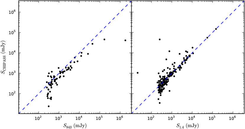
Figure 4: The CHIPASS beam-weighted flux density versus the SUMSS/MGPS-2 (left) and NVSS (right) total flux density for 204 galaxies in our sample. $y(x)=x$ is indicated by the dashed blue line.

3.5.2 Velocity width

We assign a uniform prior to the line FWHM in the velocity range 0.1–2000 km s^-1. Since the spectral channel separation and resolution of the HIPASS data are approximately 13 and 18 km s^-1, respectively, we choose a minimum value of 0.1 km s^-1 to provide sufficient sampling of this parameter for unresolved spectral lines. The maximum value of 2000 km s^-1 is set by the typical maximum widths of absorption lines observed in the literature (e.g. Morganti et al. 2005); significantly larger values would lead to confusion with the broad baseline ripples often present in radio spectra.

3.5.3 Peak depth

The maximum possible depth of a single absorption line is set by the physical constraint that the fractional absorption cannot exceed 100 per cent of the continuum flux density. By using existing measurements of the total flux density for each radio source, we can set an upper limit on the peak absorption depth. Reliable measurements of the flux densities of our radio sources at either 843 MHz and/or 1.4 GHz are available from the SUMSS/MGPS-2 and NVSS surveys, and in most cases their total flux densities have been compiled by van Velzen et al. (2012). However, since these continuum surveys were carried out at different epochs to that of HIPASS, it is possible that in some cases the continuum flux density might have varied significantly. We therefore supplement our knowledge of the continuum with the recently published 1.4 GHz Continuum HIPASS (CHIPASS; Calabretta et al. 2014) compact source map. This all-sky image has a gridded beamwidth of 14.4 arcmin and covers the same region of sky as the HIPASS 21 cm line data.

To estimate the continuum flux density that was originally subtracted from the HIPASS data, we convolve the CHIPASS image with a Gaussian smoothing kernel, effectively reducing the spatial resolution to the HIPASS beamwidth of 15.5 arcmin. We then estimate the continuum flux density within a single HIPASS beam using the weighted sum used to generate the 21 cm spectra (see Section 3.1). These CHIPASS beam-weighted flux densities for our sample of galaxies are given in Table LABEL:table:full_sample. The CHIPASS beam is almost 20 times larger than that of SUMSS, MGPS-2 and NVSS and as such we expect there to be significant confusion with other companion radio sources. Furthermore, for some sources the radio emission is significantly extended beyond the HIPASS beamwidth and so we expect the CHIPASS beam-weighted flux density to be lower than that of the total flux density given by van Velzen et al. (2012). In Fig. 4, we show the CHIPASS beam-weighted flux density versus the SUMSS/MGPS-2 and NVSS total flux densities. This plot indicates that there is general agreement between these quantities and the scatter is consistent with the aforementioned issues of confusion and extension beyond the HIPASS beam. Since we only wish to estimate the maximum possible value that the absorption-line depth parameter can take, we use the larger of the SUMSS/MGPS-2, NVSS and CHIPASS flux densities. We set the lower prior value by 1 per cent of the mean noise in the spectrum, thereby ensuring the possible detection of broad, weak absorption lines (see e.g. Allison et al. 2013) and good sampling of the depth parameter.

3.6 Calibration error

The flux density scale for HIPASS was calibrated using observations of Hydra A and PKS 1934-638, which have known values relative to the absolute scale of Baars et al. (1977). The rms variation in the HIPASS flux calibration was reported by Zwaan et al. (2004) to be 2 per cent over the duration of the southern survey. If we assume that the original flux densities obtained using the scale of Baars et al. (1977) have an accuracy of approximately 5 per cent, then we estimate that the HIPASS spectra should have a calibration error given by the quadrature sum of these two errors, approximately 5.4 per cent. To propagate this error into our analysis, we introduce a parameter that multiplies the model data at each iteration and which has a prior probability given by a normal distribution with mean equal to unity and $1\,\sigma$ width equal to $0.054$. In determining the uncertainties in our model parameters, we marginalize over this parameter.

Table 1: A summary of derived parameters for four galaxies in which we have detected H i absorption using HIPASS. $cz_{\mathrm{sys}}$ is the systemic redshift, and $S_{\rm 1.4}$ is the 1.4 GHz total flux density from NVSS (Condon et al., 1998; van Velzen et al., 2012). The parameters estimated from model fitting are as follows: $cz_{\mathrm{peak}}$ is the 21 cm redshift at peak absorption; $\Delta{S}_{\rm peak}$ is the peak absorption depth; $\Delta{v_{\mathrm{eff}}}$ is the rest effective width (as defined by Equation 20); $\tau_{\mathrm{peak}}$ is the peak optical depth, calculated using $S_{\rm 1.4}$ for the continuum component and assuming that the covering factor $f=1$ (and is therefore a lower limit to the true optical depth); $\int{\tau\,\mathrm{d}v}$ is the rest-frame velocity-integrated optical depth; $N_{\mathrm{HI}}$ is the H i column density assuming a spin temperature of 100 K; $R$ is the detection statistic as defined by Equation 15. All uncertainties are given for the 68.3 per cent interval. The dominant source of uncertainty in $S_{1.4}$ for these sources is the absolute flux calibration error (approximately 3 per cent for NVSS; Condon et al. 1998). Given that HIPASS and NVSS are both ultimately calibrated to the scale of Baars et al. (1977), we assume a strong correlation with the variance in $\Delta{S}_{\rm peak}$ and so do not propagate the uncertainty in $S_{1.4}$ through to our estimate of the peak optical depth and its dependent quantities.

Name	$cz_{\mathrm{sys}}$	$S_{\rm 1.4}$	$cz_{\mathrm{peak}}$	$\Delta{S}_{\rm peak}$	$\Delta{v_{\mathrm{eff}}}$	$\tau_{\rm peak}$	$\int{\tau\,\mathrm{d}v}$	$N_{\rm HI}$	$R$
	(km s-1)	(mJy)	(km s-1)	(mJy)	(km s-1)		(km s-1)	($10^{20}$ cm-2)
2MASX J13084201-2422581	$4257\pm 45$	$474\pm 14$	$4224.4_{-2.7}^{+2.7}$	$109_{-10}^{+11}$	$71.0_{-6.7}^{+6.9}$	$0.26_{-0.03}^{+0.03}$	$17.8_{-1.7}^{+1.8}$	$32.4_{-3.0}^{+3.4}$	$104.6\pm 0.1$
Centaurus A	$547\pm 5$	$4520\pm 226$$a$	$548.7_{-0.5}^{+0.6}$	$1690_{-550}^{+770}$	$7.4_{-2.3}^{+3.6}$	$0.47_{-0.18}^{+0.32}$	$3.1_{-0.2}^{+0.3}$	$5.7_{-0.4}^{+0.5}$	$898.9\pm 0.3$
NGC 5793	$3491\pm 66$	$1200\pm 36$	$3516.6_{-1.4}^{+1.2}$	$880_{-47}^{+48}$	$109.3_{-2.1}^{+2.1}$	$1.32_{-0.14}^{+0.16}$	$116_{-9}^{+11}$	$211_{-17}^{+19}$	$11\,090.0\pm 0.3$
Arp 220	$5434\pm 7$	$326\pm 10$	$5477_{-15}^{+16}$	$42.5_{-4.5}^{+4.7}$	$375_{-41}^{+46}$	$0.14_{-0.02}^{+0.02}$	$51.2_{-5.5}^{+6.2}$	$93_{-10}^{+11}$	$77.0\pm 0.1$

• Centaurus A has significantly extended 1.4 GHz continuum emission with respect to the HIPASS beamwidth and so we use the core flux density measured by Tingay et al. (2003) to estimate the peak optical depth and its dependent quantities. We assume that the dominant source of uncertainty for this measurement is the absolute flux calibration error of 5 per cent given by Tingay et al.

3.7 Derived quantities

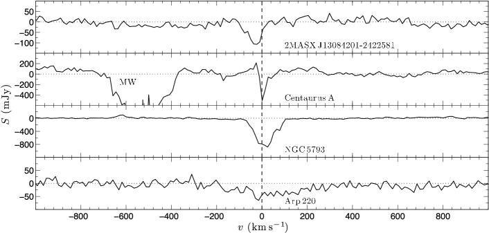
Figure 5: HIPASS spectra at the position of four galaxies in which we have detected absorption. The radial velocity axis is given relative to the rest frame defined by the systemic redshift of the host galaxy (see Table LABEL:table:full_sample). The absorption in 2MASX J13084201-2422581 was previously unknown. The broad feature ($v\sim-600$ km s^-1) towards Centaurus A is consistent with being Galactic in origin.

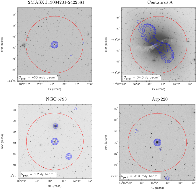
Figure 6: Radio and optical images of the four galaxies in which we have detected absorption using HIPASS. The blue contours denote the 1, 2, 5, 10, 20, 50 per cent levels of the peak radio flux density within the HIPASS beamwidth, from either NVSS ($\delta>-30\degr$) or SUMSS/MGPS-2 ($\delta<-30\degr$). For clarity we exclude those radio contours that are less than five times the survey rms. The large red circle represents the gridded HIPASS beamwidth of 15.5 arcmin. The grey-scale images represent optical $B_{j}$-band photometry from the SuperCosmos Sky Survey, using the UK Schmidt and Palomar Oschin Schmidt telescopes (Hambly et al., 2001).

Model parametrization allows us to estimate those properties of the absorption that we are interested in. In the regime where the background source is significantly brighter than foreground H i emission, the 21 cm optical depth across the line profile, $\tau(v)$, can be recovered from the absorption ($\Delta{S}$) of the continuum ($S_{\mathrm{cont}}$) by

$$\tau(v)=-\ln\left[1-{1\over f}\left({\Delta{S(v)}\over{S_{\mathrm{cont}}(v)}}\right)\right],$$ (18)

where $f$ (the covering factor) is the fractional projected area of continuum obscured by the absorbing gas, and $v$ is the velocity with respect to the rest frame of the system. It should be noted that throughout this work we assume that $f=1$, so that estimates of $\tau$ are a lower limit to the true optical depth. The column density of H i gas ($N_{\rm HI}$, in units of ${\rm cm}^{-2}$) can be estimated from the velocity- integrated optical depth (in units of ${\rm km\,s}^{-1}$) using the following relationship (e.g. Wolfe & Burbidge, 1975),

$$N_{\mathrm{HI}}=1.823\times 10^{18}~{}T_{\mathrm{spin}}~{}\int{\tau(v)~{}\mathrm{d}v},$$ (19)

where the spin temperature, $T_{\mathrm{spin}}$ (in units of K), is the excitation temperature for the 21 cm transition and hence a measure of the relative populations of the two hyperfine states of the hydrogen 1s ground level. $T_{\mathrm{spin}}$ is determined by both radiative and collisional processes, converging to the kinetic temperature for a collision dominated gas (e.g. Purcell & Field 1956; Field 1958, 1959).

For the purpose of comparing the widths of absorption lines, we define the rest effective width (see also Dickey 1982 and Allison et al. 2013) as

$$\Delta{v}_{\mathrm{eff}}\equiv\left[\int{{\Delta{S}(v)\over{S_{\mathrm{cont}}(v)}}~{}\mathrm{d}v}\right]\Big{/}\left({\Delta{S}\over{S_{\mathrm{cont}}}}\right)_{\mathrm{\!peak}},$$ (20)

where $v$ is the rest-frame radial velocity (referenced with respect to the systemic redshift) and $(\Delta{S}/S_{\mathrm{cont}})_{\mathrm{peak}}$ is the peak fractional absorption. This quantity has advantages over both the FWHM and the full-width at zero intensity, since it is more representative of the width of complex multicomponent line profiles, which might have broad and shallow wings, and is not as strongly influenced as by the S/N.

3.8 Detections

Using the automated method outlined above, we obtain 51 potential detections of absorption-like features in our 204 HIPASS spectra. Further visual inspection of all the spectra confirms that 47 are likely to be false positives, which in some cases were rejected due to their low significance ($R\lesssim 1$) relative to the continuum-only hypothesis. However, the majority are found to be associated with negative features generated by spectral baseline ripples, which are significant compared to the noise. It is clear from these results that when such strong spectral baseline ripples are present, the most effective and robust methods of absorption-line detection are to either use an automated method followed by visual inspection, as was done here, or to account for the effect of these nuisance signals a priori using the covariance matrix. After rejecting these false positives, we are left with four detections that we classify as real H i absorption lines, associated with four nearby galaxies.

In Table 1, we summarize the H i parameters derived from model fitting to the HIPASS spectra. In Figs 5 and 6, we show the spectra and images, respectively, at the positions of the four galaxies. Of these detections, three were previously known: Centaurus A (Roberts, 1970), NGC 5793 (Jenkins, 1983) and Arp 220 (Mirabel, 1982), while the fourth, 2MASX J13084201-2422581, was not previously reported in the literature. It should be noted that while the first three galaxies are common to both samples, 2MASX J13084201-2422581 is only listed in Sample 1, since its 2MASS $K_{s}$-band magnitude ($K_{s}=11.8$) was not bright enough to be included in the catalogue of van Velzen et al. (2012). We discuss further the results of the model parametrization and inferred properties of the H i absorption in Section 5.1.

4 Followup with the ATCA

4.1 Observations

We examined further the 21 cm absorption seen in 2MASX J13084201-2422581 and NGC 5793 by re-observing these galaxies with the Australia Telescope Compact Array (ATCA) Broadband Backend (CABB; Wilson et al., 2011) in 2013 February 13–16. Our aims were twofold: to confirm the new detection of H i absorption in 2MASX J13084201-2422581 and to verify the tentatively detected broad absorption wings seen towards NGC 5793 by Koribalski (2012).

Observations were carried out in a similar manner to those reported by Allison et al. (2012a, 2013). We used the 64 MHz zoom band capability of CABB to position 2048 spectral channels (with velocity resolution $\sim 6.7$ km s^-1) at a centre frequency of 1406 MHz, equivalent to 21 cm redshifts in the range $-3\,670\lesssim cz\lesssim 10\,130$ km s^-1. This band provides almost three times the spectral resolution of HIPASS, and comfortably includes the redshifts of the two galaxies. The six-element ATCA was arranged in the 6A east-west configuration with baselines in the range 0.337–5.939 km. At 1406 MHz, this configuration provides an angular scale sensitivity range of 7–130 arcsec and a primary beam FWHM of approximately 35 arcmin. Short scans of the target fields were interleaved with regular observations of nearby bright point sources for gain calibration (PKS 1308-220 and PKS 1504-166), with a total on-target integration time of 2 h 30 min for 2MASX J13084201-2422581 and 2 h 15 min for NGC 5793. We observed PKS 1934-638 for calibration of the band-pass and absolute flux scale.

4.2 Data reduction

The ATCA data were flagged, calibrated and imaged in the standard way using tasks from the Miriad package (Sault et al., 1995). Manual flagging was performed using the task Uvflag for known radio frequency interference (RFI) in 80 channels at 1381 MHz (from mode L3 of the Global Positioning System) and 60 channels at 1431 MHz (from the 1.5 GHz terrestrial microwave link band), as well as 20 channels for the 1420 MHz Galactic 21 cm signal. The remaining 1888 channels were automatically flagged for transient glitches and low-level RFI using iterative calls to the task Mirflag, resulting in less than 2 per cent of the data per channel being lost. Initial calibration was performed using bright calibrator sources, to correct the band-pass, gains and absolute flux scale. Further correction of the gain phases was performed using self-calibration based on a continuum model of each target field. Continuum models were generated using the multi-frequency deconvolution task, Mfclean, which recovers both the fluxes and spectral indices of the brightest sources in the field. The NVSS catalogue ($S_{1.4}\gtrsim 2.5$ mJy; Condon et al. 1998) was used to identify the positions of these sources.

Initially, we imaged the target fields by uniformly weighting the calibrated visibilities, thereby favouring the undersampled longer baselines and so optimizing the spatial resolution. However, from visual inspection of these uniformly weighted images, we found that the target sources are only resolved on scales smaller than the synthesized beam FWHM of $\sim$ 10 arcsec. Based on this information, we instead used the natural weighting scheme to generate our final continuum and spectral images, which optimizes the S/N for detection. Before constructing our final data cubes, we subtracted a continuum model of other nearby sources in the field, thereby removing significant spectral baseline artefacts generated from incomplete Fourier sampling. A spectrum was then extracted from each data cube at the position of the target source, using the method described in Section 3.1 for an elliptical synthesized beam. In Table 2, we summarize some properties of our ATCA observations and in Figs 7 and 8 we show the final CABB spectra and images, respectively, for both targets. Note that our analysis method does not require any smoothing of the spectral data.

Table 2: A summary of our ATCA observations, where $t_{\rm int}$ is the total integration time on each source; $\theta_{\rm maj}$, $\theta_{\rm min}$ and $\phi$ are the major axis, minor axis and position angle, respectively, of an elliptical fit to the synthesized beam; and $\sigma_{\mathrm{chan}}$ is the per-channel noise estimate in the CABB spectra.

Name	$t_{\rm int}$	$\theta_{\rm maj}$	$\theta_{\rm min}$	$\phi$	$\sigma_{\mathrm{chan}}$
	(hh:mm)	(arcsec)		(deg)	(mJy)
2MASX J13084201-2422581	02:30	19.5	9.2	-5.2	3.2
NGC 5793	02:15	28.6	8.5	-7.9	3.9

Table 3: A summary of derived H i absorption parameters for 2MASX J13084201-2422581 and NGC 5793, estimated from our CABB 21 cm spectra. $S_{\mathrm{cont}}$ is the continuum flux density at the position of peak absorption and $\chi_{\rm ml}^{2}/{\rm d.o.f.}$ is the reduced chi-squared statistic for the maximum likelihood model parameters; the other parameters are as defined in Table 1. All uncertainties are given for the 68.3 per cent interval.

Name	$S_{\mathrm{cont}}$	$cz_{\mathrm{peak}}$	$\Delta{S}_{\rm peak}$	$\Delta{v_{\mathrm{eff}}}$	$\tau_{\rm peak}$	$\int{\tau\,\mathrm{d}v}$	$N_{\mathrm{HI}}$	$R$	$\chi_{\rm ml}^{2}/{\rm d.o.f.}$
	(mJy)	(km s-1)	(mJy)	(km s-1)		(km s-1)	(  $10^{20}$ cm-2)
2MASX J13084201-2422581	$499_{-32}^{+35}$	$4238.0_{-3.5}^{+2.0}$	$122.5_{-8.0}^{+8.6}$	$86.8_{-2.2}^{+2.2}$	$0.28_{-0.01}^{+0.01}$	$23.3_{-0.4}^{+0.5}$	$42.5_{-0.8}^{+0.8}$	$6061.8\pm 0.3$	$1.22\pm 0.03$
NGC 5793	$1022_{-73}^{+77}$	$3514.9_{-0.4}^{+0.4}$	$922_{-67}^{+69}$	$97.7_{-0.3}^{+0.3}$	$2.32_{-0.03}^{+0.03}$	$157.6_{-0.5}^{+0.5}$	$287.2_{-1.0}^{+1.0}$	$270\,809.6\pm 0.3$	$1.08\pm 0.03$

4.3 CABB data analysis and modelling

We determine best-fitting models of the H i absorption in each CABB spectrum using the Bayesian method described in Section 3.4. The continuum component is parametrized using a first-order polynomial (linear) model and the absorption line by the combination of multiple Gaussian components. The best-fitting number of Gaussian components is then optimized by maximizing the statistic $R$ (Equation 15). We assume that the CABB data have a rectangular spectral point spread function, so that the channels are independent of each other (Wilson et al., 2011) and hence the covariance matrix C in Equation 17 reduces to the on-diagonal set of channel variances, estimated using the MADFM statistic over the spectrum.

While it is reasonable to assume that the CABB spectra are free of strong spectral baseline artefacts, we again use a normal probability distribution for the position of the absorption line, centred on the systemic redshift and within the 1$\sigma$ width of $\pm 50$ km s^-1. We do this for two reasons: to encode our prior belief that the absorption should arise near the known systemic redshift, and to avoid unnecessarily fitting to any broad and shallow spectral baseline ripples that might exist at either edge of the spectrum. The FWHM of each Gaussian component is given a uniform prior of 0.1–2000 km s^-1, and the lower and upper limits of the depth are set by 1 per cent of the per-channel noise and the mean continuum flux density, respectively. We assume a systematic error of $\pm$10 per cent for the calibration procedure, which is approximated by multiplying the model data by an additional parameter with a normal prior of $1.0\pm 0.1$. While this nuisance parameter increases the uncertainty in our estimates of the absolute flux scale of the continuum and spectral line components, it does not significantly alter the relative fractional absorption. A summary of the estimated H i parameters from model fitting to the CABB spectra is given in Table 3. In Table 4 and Fig. 9 we summarize the best-fitting parameters, for multiple Gaussian components, for both the HIPASS and CABB data.

5 Discussion

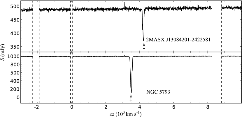
Figure 7: CABB 21 cm spectra showing both continuum emission and H i absorption at the positions of radio sources hosted by 2MASX J13084201-2422581 and NGC 5793. The arrow and horizontal line indicate the mean and uncertainty in the systemic redshift. The vertical dashed lines enclose those spectral channels that were flagged either due to persistent strong RFI or Galactic 21 cm signal. The emission spike that is apparent in both spectra, within a single channel at the band centre (1406 MHz, $cz\approx 3100\,\mathrm{km}\,\mathrm{s}^{-1}$), arises due to self-generated interference within the telescope (see Wilson et al. 2011).

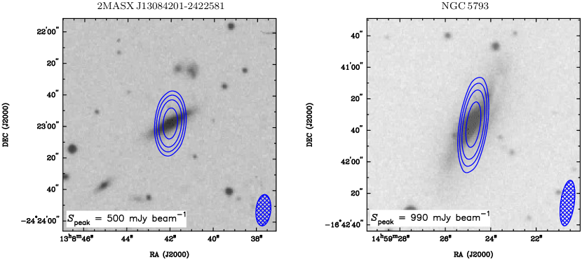
Figure 8: 1.4 GHz ATCA images of 2MASX J13084201-2422581 and NGC 5793, where the blue contours denote the 5, 10, 20, 50 per cent levels of the peak continuum flux density. The FWHM of the synthesized beam is shown in the bottom-right corner. The grey-scale images represent optical $B_{j}$-band photometry from the SuperCosmos Sky Survey, using the UK Schmidt and Palomar Oschin Schmidt telescopes (Hambly et al., 2001).

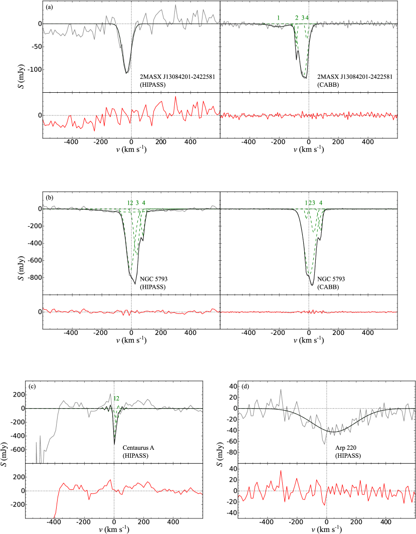
Figure 9: The best-fitting models of HIPASS and CABB spectra in which we have detected associated H i absorption. The radial velocity axis is given relative to the rest frame defined by the systemic redshift (vertical dotted line). For the CABB spectra, the grey line represents the data after we have subtracted our best-fitting continuum component, whereas for the HIPASS spectra the grey line represents the original baseline-subtracted data. The solid black line represents the best-fitting spectral line model and the dashed green lines the individual Gaussian components (top panel). The solid red line represents the best-fitting residual (bottom panel).

5.1 Individual sources

5.1.1 2MASX J13084201-2422581

We detect a previously unknown 21 cm absorption line against the compact flat-spectrum radio source at the centre of the Seyfert 2 galaxy 2MASX J13084201-2422581. We show in Fig. 9 the best fitting models to both the HIPASS and CABB spectra. By comparing the marginal likelihoods for increasingly complex models, we find that the HIPASS data warrant only a single-component Gaussian model, while a four-component model is favoured by the CABB data. The similarity in our estimates of the peak depth and rest effective width for each spectrum implies that all of the H i absorption detected within the 15.5 arcmin HIPASS beam arises from a region of angular size smaller than the ATCA synthesized beam, which at $cz=4257$ km s^-1 equates to a projected physical size smaller than $6\times 3$ kpc. This result is consistent with the compact morphology of the radio source at 1.4 GHz, evident from the NVSS and ATCA images, and the absence of other nearby strong radio sources within the HIPASS beam (see Fig. 6).

The redshift of the peak absorption is consistent with the systemic redshift of the host galaxy, implying that the bulk of the cold H i gas is not rapidly infalling or outflowing with respect to ionized gas in the nucleus. The stellar component of the host galaxy exhibits an edge-on irregular spiral morphology at near-infrared and optical wavelengths (Jarrett et al., 2000; Hambly et al., 2001), which, with the Seyfert 2 classification of the AGN, suggests that the bulk of the absorbing gas may arise within an obscuring disc of H i gas. While we cannot spatially resolve the background radio-jet structure with our ATCA observations, and hence strongly constrain the spatial distribution and kinematics of the H i gas, we note that the shape and width of the absorption-line profile are very similar to those observed in other Seyfert galaxies (e.g. Dickey 1982, 1986; Gallimore et al. 1999). Work by Gallimore et al. (1999) showed that these systems are well modelled by sub-kpc discs of H i gas that are typically aligned with the outer stellar disc. Deviations in the regular shape of the main profile (components 2, 3 and 4 in Fig. 9) are likely generated by a combination of unresolved spatial variations in the optical depth of the gas, the complex geometries of the absorber-radio source system and radial streaming of the gas with respect to the source. The separate broad and shallow blueshifted component at $v\sim 200\,\mathrm{km}\,\mathrm{s}^{-1}$ indicates that gas might be caught in a jet-driven outflow on sub-kpc scales, but this interpretation remains tentative until the absorption can be spatially resolved.

Our best estimates of the peak and integrated 21 cm optical depths from the CABB data are $0.28\pm 0.01$ and $23.3\pm 0.5$ km s^-1, respectively (assuming that $f=1$). However, without further knowledge of the relative size and geometry of the absorbing gas with respect to the continuum source, as well as the spin temperature of gas, it is very difficult to obtain an accurate measurement of the column density from Equation 19. Gallimore et al. (1999) showed that for a dense AGN-irradiated gas cloud in the narrow-line region of a Seyfert galaxy, the 21 cm spin temperature is likely to be collisionally dominated with typical values of $T_{\mathrm{spin}}=100$ K. However, if the sightline to the continuum source intercepts the warmer atomic medium, then the spin temperature may be much higher. For example, 21 cm observations of intervening damped Lyman $\alpha$ absorbers ($N_{\mathrm{HI}}>2\times 10^{20}\,\mathrm{cm}^{-2}$) show that $T_{\mathrm{spin}}/f$ can be greater than $1000\,\mathrm{K}$ (see Curran 2012 and references therein). Furthermore, if the H i gas in this Seyfert 2 galaxy is distributed as a disc on scales less than 100 pc, then it would be unlikely that all of the source structure would be uniformly obscured by the absorbing gas, and so in this case we would expect the covering factor to be less than unity. Therefore, given the possible values of $T_{\mathrm{spin}}$ and $f$, we can only estimate a lower limit to the H i column density of $N_{\mathrm{HI}}=42.5\pm 0.8\times 10^{20}~{}(T_{\mathrm{spin}}/100\,\mathrm{K})~{}\mathrm{cm}^{-2}$. The stellar disc evident in the 2MASS $K_{s}$-band photometry for this galaxy has a major–minor axis ratio of 0.380 (Jarrett et al., 2000), which we convert into an inclination angle of $i=74\degr$ (Tully & Fisher, 1977; Aaronson et al., 1980). Assuming that the H i gas is coplanar with the stellar component, our estimate of the column density is consistent with the inclination angle relationship measured in other Seyferts and active galaxies by Dickey (1982, 1986) and Gallimore et al. (1999).

Table 4: Best-fitting parameters from fitting multiple Gaussian components to the HIPASS and CABB 21 cm spectra. $n$ is the component number, corresponding to the label given in Fig. 9; $cz$ is the component redshift; $\Delta{v_{\rm FWHM}}$ is the velocity FWHM and $\Delta{S}$ is the depth.

Name	Data	$n$	$cz$	$\Delta{v_{\rm FWHM}}$	$\Delta{S}$
			(km s-1)	(km s-1)	(mJy)
2MASX J13084201-2422581	HIPASS	1	4224	66	102
	CABB	1	4050	127	6
		2	4170	12	53
		3	4219	65	114
		4	4243	18	36
Centaurus A	HIPASS	1	548	3	2686
		2	564	21	241
NGC 5793	HIPASS	1	3484	63	702
		2	3486	380	36
		3	3526	39	544
		4	3569	25	325
	CABB	1	3474	15	143
		2	3496	83	848
		3	3525	35	310
		4	3570	24	298
Arp 220	HIPASS	1	5482	348	42

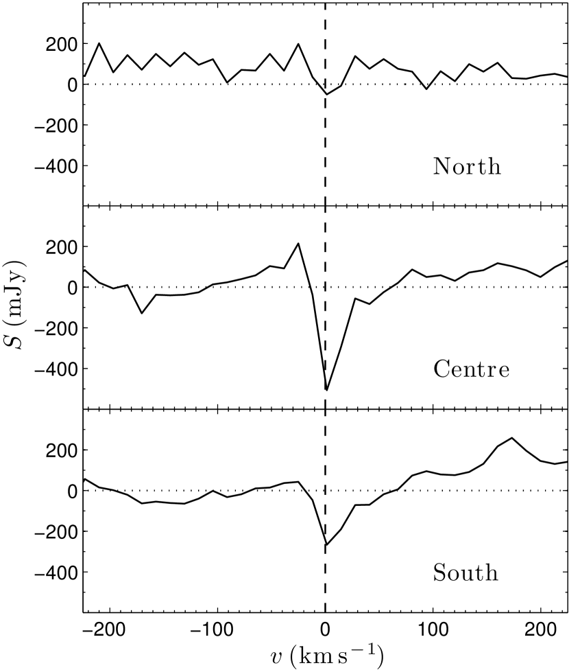
Figure 10: HIPASS spectra towards Centaurus A, extracted at 15.5 arcmin separations along the observed jet-axis, at RA (J2000) = $13^{\rm h}26^{\rm m}27\aas@@fstack{s}72$, Dec. (J2000) = $-42\degr 50\arcmin 09\aas@@fstack{\prime\prime}8$ (north), RA (J2000) = $13^{\rm h}25^{\rm m}27\aas@@fstack{s}76$, Dec. (J2000) = $-43\degr 01\arcmin 07\aas@@fstack{\prime\prime}4$ (centre) and RA (J2000) = $13^{\rm h}24^{\rm m}27\aas@@fstack{s}80$, Dec. (J2000) = $-43\degr 12\arcmin 05\aas@@fstack{\prime\prime}0$ (south). The radial velocity axis is given relative to the rest frame defined by the systemic redshift (vertical dashed line).

5.1.2 Centaurus A

Centaurus A (NGC 5128) is by far the closest early-type radio galaxy to the Milky Way, which at a distance of only 3.8 Mpc (Harris et al., 2010) has been imaged in detail at multiple wavelengths (see Israel 1998 and references therein). In the HIPASS spectrum, extracted from the core of the radio source, we re-detect the H i absorption first discovered by Roberts (1970) and studied extensively since (e.g. Whiteoak & Gardner, 1971; van der Hulst et al., 1983; Sarma et al., 2002; Morganti et al., 2008; Struve et al., 2010). Due to the proximity and radio power ($P_{1.4}\approx 5\times 10^{24}$ W Hz^-1) of this source, the HIPASS spectrum is strongly contaminated by the spectral baseline ripple. Despite this, we recover a two-component Gaussian model of the line (Fig. 9c), with an effective width of $7.4_{-2.3}^{+3.6}$ km s^-1 and a peak depth of $1690_{-550}^{+770}$ mJy. The poor constraints on these parameter estimates, compared with those for the other detections, are the result of low spectral sampling across the line.

The structure of the line profile, with a deep narrow component at the systemic redshift and an broadened component towards higher redshifts, is consistent with the structure seen at similar spectral and spatial resolution by Roberts (1970) and Whiteoak & Gardner (1971). The deeper narrow component is thought to arise in absorption from H i gas in a rotating disc that is coplanar with the prominent warped dust lane, while some of the redshifted absorption is consistent with infalling clouds towards the nucleus (van der Hulst et al., 1983; Sarma et al., 2002). Higher spatial resolution and more sensitive observations by Morganti et al. (2008) and Struve et al. (2010) revealed blueshifted absorption towards the nucleus, potentially indicating the presence of a circumnuclear disc of H i on sub-100 pc scales.

The 1.4 GHz emission from Centaurus A is moderately extended with respect to the HIPASS beam, and so in Fig. 10 we show spectra extracted at three positions along the observed jet axis, separated by intervals of 15.5 arcmin. While evidently contaminated by residual spectral baseline signal, and subject to adjacent signal entering from the beam sidelobes, we tentatively see more absorption towards the southern end of the jet axis. This is consistent with the orientation of the H i disc against the southern radio lobe, seen at higher spatial resolution (e.g. Struve et al., 2010).

5.1.3 NGC 5793

The very deep 21 cm absorption seen towards the compact and radio-luminous nucleus in this edge-on disc Seyfert 2 galaxy was first detected by Jenkins (1983) using the 64 m Parkes Radio Telescope, and has since been studied at higher spatial resolution by Gardner & Whiteoak (1986) using the Very Large Array (VLA), and by Gardner et al. (1992) and Pihlström et al. (2000) using very long baseline interferometry (VLBI). The absorption-line profile seen in the HIPASS spectrum (Koribalski et al., 2004) is consistent with that observed by Jenkins (1983). The weaker emission-line feature seen in both spectra at $cz\approx 2860$ km s^-1 is attributed by Koribalski (2012) to H i gas in the neighbouring dwarf irregular galaxy 6dF J1459410-164235 (to the east), and not the E0 galaxy NGC 5796 (to the north), which is thought to be relatively H i poor.

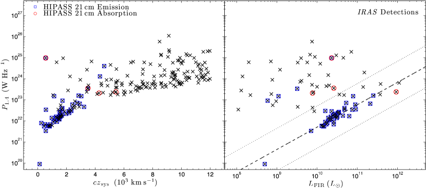
Figure 11: Left: the 1.4 GHz radio power versus the systemic redshift for all 204 galaxies in our sample. Right: the 1.4 GHz radio power versus the far-infrared luminosity for those 86 galaxies with far-infrared 60 or 100 $\mathrm{\mu}$m flux densities from the IRAS survey. The blue squares represent those galaxies with H i emission catalogued in HIPASS and the red circles denote those in which we have detected absorption. The dashed line shows the radio power versus far-infrared luminosity relationship measured by Mauch & Sadler (2007) for star-forming galaxies. The dotted lines indicate a one-decade deviation from this relationship.

The spatially unresolved absorption lines in both our HIPASS and CABB spectra clearly exhibit some velocity structure, which we successfully model using a four-component Gaussian model (see Fig. 9b). VLBI observations by Pihlström et al. (2000) demonstrated that this structure results from the superposition of individual H i components seen against two continuum sources that are only resolved on angular scales smaller than 10 mas. They suggest that the broadest feature likely arises in a nearly edge-on disc of H i gas ($i\approx 73\,\degr$), and occurs on scales of 50–100 pc from the AGN, consistent with that seen in other Seyfert 2s (Gallimore et al., 1999), while the other features are signatures of individual H i clouds that are either interior or exterior to this disc. By fitting a four component Gaussian model to the CABB spectrum, we estimate that the peak and integrated optical depth are $2.32\pm 0.03$ and $157.6\pm 0.5$ km s^-1, respectively, giving a total H i column density of $N_{\mathrm{HI}}=287.2\pm 1.0\times 10^{20}(T_{\mathrm{spin}}/100\,\mathrm{K})$ cm^-2. This is consistent with the total column density measured by Pihlström et al. (2000), averaged across the resolved continuum components, of $N_{\mathrm{HI}}\approx 3.5\times 10^{22}(T_{\mathrm{spin}}/100\,\mathrm{K})$ cm^-2.

Koribalski (2012) tentatively identified a previously undetected broad absorption feature in the HIPASS spectrum, with a width of $680$ km s^-1 and centred on the systemic redshift. Using Bayesian model comparison, we confirm that this feature is statistically significant above the noise (component 1 in Fig. 9b and Table 4); however, it is not clear if this feature is distinguishable from other residual baseline features seen in the spectrum. Furthermore, we do not re-detect this broad component in the CABB spectrum (with an estimated per-channel noise of $\sigma_{\rm chan}=3.9$ mJy), even though there is strong consistency between the other absorption components seen in both spectra. It is plausible that this feature could have arisen towards a confused source within the HIPASS beam, from H i gas that is at a similar redshift to NGC 5793. There are two other sources within the HIPASS beam that have sufficient flux densities ($S_{1.4}\gtrsim 35$ mJy) in the NVSS catalogue to produce such an absorption: NGC 5796 ($S_{1.4}=109$ mJy, $cz_{\rm sys}=2971$ km s^-1; Wegner et al. 2003) and MRC 1456-165 ($S_{1.4}=379$ mJy). However, spectra extracted from the CABB data at the centroid positions of both sources show no evidence of the broad absorption seen in the HIPASS spectrum. We therefore conclude that this feature is likely an artefact and the result of residual spectral baseline ripple in the HIPASS spectrum.

5.1.4 Arp 220

The broad absorption-line associated with this prototypical ultraluminous infrared galaxy (Sanders et al. 2003) was originally detected by Mirabel (1982), using the 300 m Arecibo Telescope, and has since been re-observed and studied multiple times (e.g. Dickey 1986; Baan et al. 1987; Garwood et al. 1987; Baan & Haschick 1995; Hibbard et al. 2000; Mundell et al. 2001). We find that the line detected in the HIPASS spectrum requires only a single-component Gaussian model, with an effective width ($\Delta{v_{\rm eff}}=375_{-41}^{+46}$ km s^-1) and peak depth ($\Delta{S_{\rm peak}}=42.5_{-4.5}^{+4.7}$ mJy) that are consistent with previous single-dish observations (e.g Mirabel 1982; Garwood et al. 1987). However, the lower S/N and spectral resolution of the HIPASS spectrum means that we do not find as much structure in the line as seen in these other single-dish observations.

The absorption arises from gas towards a compact radio-loud nucleus that consists of two distinct components (e.g. Baan et al. 1987; Norris 1988; Baan & Haschick 1995), which are thought to be the nuclei of two gas-rich progenitor galaxies in an advanced stage of merging. At 1.4 GHz, they are only resolved on angular scales smaller than $\sim 200$ mas (Mundell et al., 2001) and are therefore not resolved by HIPASS. Mundell et al. carried out a high spatial resolution study of the 21 cm line on sub-arcsec scales, using the Multi-Element Radio-Linked Interferometer Network array, and showed that the bulk of the absorption is likely associated with two counterrotating discs of H i gas centred on each of the nuclei, consistent with observations of emission from the CO gas content (Sakamoto et al., 1999). The broad width of the absorption line seen in the HIPASS spectrum is consistent with the superposition of these rotating components and the bridge of H i gas connecting the two nuclei.

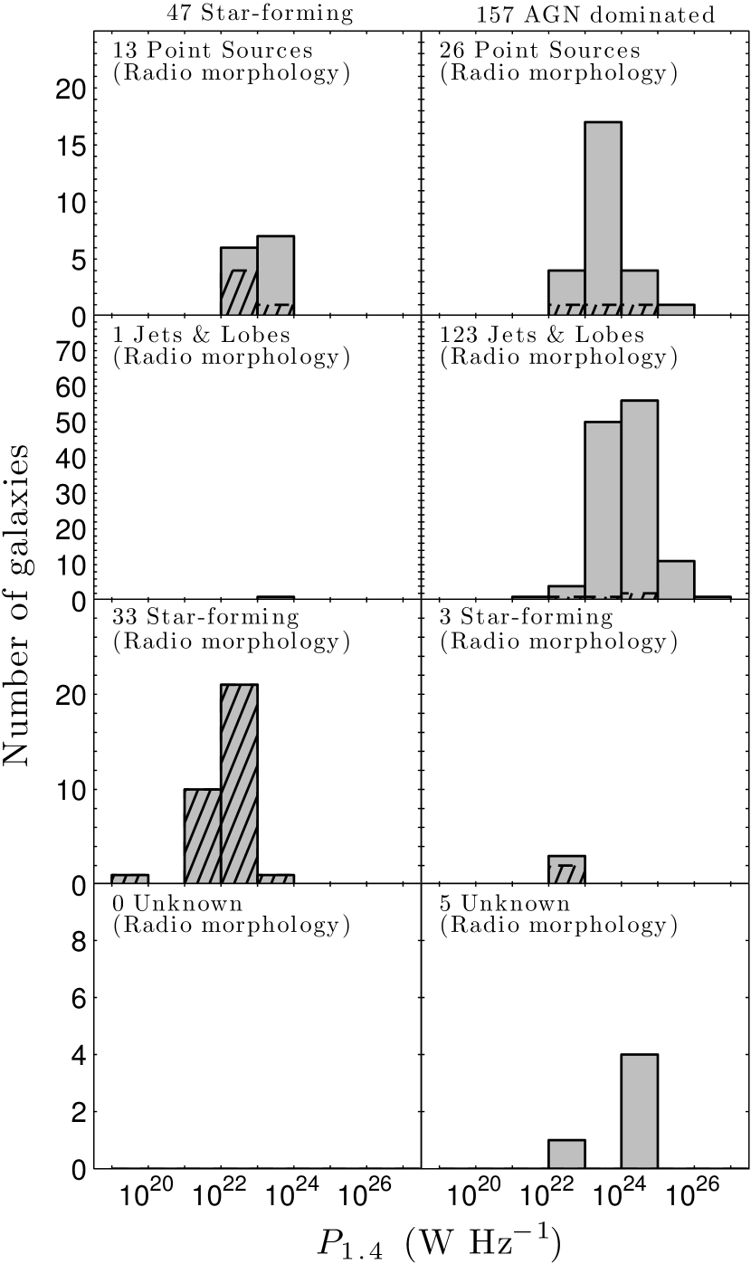
Figure 12: The distribution of 1.4 GHz radio powers for our sample, where we have classified galaxies as either star forming or AGN dominated (based on the radio and far-infrared luminosity relationship), and which have radio morphologies as classified by van Velzen et al. (2012). The hatched bars represent those galaxies with catalogued 21 cm line emission in HIPASS (Koribalski et al. 2004; Meyer et al. 2004; Wong et al. 2006).

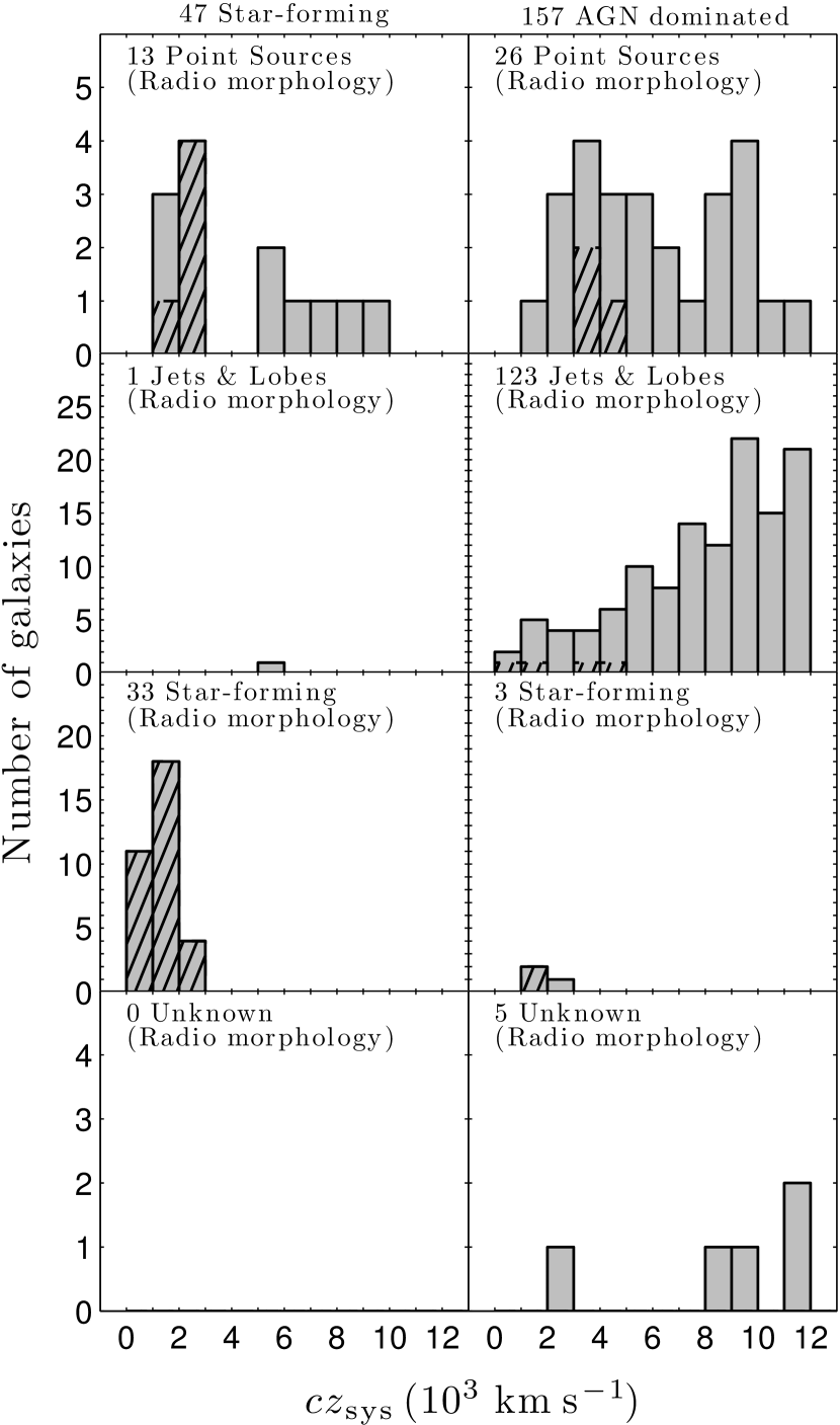
Figure 13: As Fig. 12, but for the distribution of redshifts.

5.2 Comparison with the 2 Jy sample

Morganti et al. (2001) used the ATCA, the VLA and the Westerbork Synthesis Radio Telescope to search for H i absorption in 23 radio galaxies (at $z<0.22$ and $\delta<+10\degr$) selected from the 2 Jy sample (Wall & Peacock, 1985). We can use this relatively homogeneous set of observations to determine whether our non-detections in HIPASS are consistent with what we would expect from existing detections of absorption. In five of these radio galaxies, Morganti et al. detected H i absorption, of which NGC 5090 ($cz=3421\pm 21$ km s^-1) and 3C 353 ($cz=9120\pm 59$ km s^-1) are within the volume surveyed by HIPASS. The 21 cm spectra of these two galaxies exhibit peak absorption of 8 and 10 mJy, with FWHMs of approximately 100 and 200 km s^-1, respectively. Given the noise and baseline ripple confusion in the HIPASS spectra, our non-detection of H i absorption in these radio galaxies is consistent with the expected strength of these lines.

5.3 The HIPASS detection rate

We obtain detection rates for associated absorption in HIPASS of 2.0 per cent (4/204) for the total sample, 4.4 per cent (4/90) for Sample 1 and 1.6 per cent (3/189) for Sample 2. While such a small number of detections does not allow us to draw strong conclusions about the population, we can attempt to understand these rates in the context of the HIPASS survey parameters and the properties of individual galaxies in the sample.

In Fig. 11, we show the 1.4 GHz radio power versus systemic redshift (for all 204 galaxies in our sample), and the far-infrared luminosity for those 86 galaxies that either have a detection at 60 or 100 $\mathrm{\mu}$m in the Infrared Astronomical Satellite (IRAS) Faint Source, Point Source and Galaxy Catalogues (Beichman et al., 1988; Rice et al., 1988; Knapp et al., 1989; Moshir et al., 1992; Sanders et al., 2003). The radio power is estimated using the larger of either the 843 MHz SUMSS (assuming a spectral index of $-0.6$) or 1.4 GHz NVSS total flux densities, and thereby accounting for components that might be present in SUMSS but missing in the NVSS images.

We calculate the far-infrared luminosity using an estimate of the flux density ($S_{\mathrm{FIR}}$) between 42.5 and 122.5 $\mathrm{\mu}$m, which is given by (Helou et al., 1985)

$$S_{\mathrm{FIR}}=1.26\times 10^{-14}\,(2.58\,S_{\mathrm{60\mu m}}+S_{\mathrm{100\mu m}})\,\mathrm{W\,m^{-2}},$$ (21)

where $S_{\mathrm{60\mu m}}$ and $S_{\mathrm{100\mu m}}$ are the 60 and 100 $\mu$m flux densities in units of Jy. For those galaxies where measurements of only $S_{\mathrm{60\mu m}}$ or $S_{\mathrm{100\mu m}}$ are available, we use $\langle\log_{10}(S_{\mathrm{100\mu m}}/S_{\mathrm{60\mu m}})\rangle=0.3$, which is the average calculated from the IRAS Bright Galaxy sample by Soifer et al. (1989). Galaxies that are identified as star forming exhibit a strong correlation between their radio and far-infrared luminosities (e.g Helou et al., 1985; Devereux & Eales, 1989; Condon et al., 1991). For a large sample of spectroscopically identified star-forming galaxies, Mauch & Sadler (2007) measured this relationship to be

$$\log_{10}(P_{1.4})=(1.06\pm 0.01)\log_{10}(L_{\mathrm{FIR}})+(11.1\pm 0.1),$$ (22)

with a maximum deviation in radio power of approximately one decade. We use this to identify galaxies in our sample that are star-forming, classifying AGN dominated galaxies as those that do not follow this relationship or do not have detections in both the 60 and 100 $\mathrm{\mu}$m bands.

Based on the $P_{1.4}$–$L_{\mathrm{FIR}}$ relation, we estimate that 20 per cent (47/204) of our galaxies are star forming, which is consistent with the 42 predicted using the local radio luminosity function of Mauch & Sadler (2007). Considering the relative radio and near-infrared morphologies of these star-forming galaxies, 13 are unresolved point sources, 33 have extended emission that is consistent with star formation, and only 1 is identified as having jets and lobes. For the remaining 157 galaxies in our sample, which we classify as AGN dominated, 26 are unresolved point sources, 123 are identified as having jets and lobes, 3 have extended emission consistent with star formation, and 5 have unknown structure. Hence, there is a clear consistency between the classifications based on the radio and far-infrared luminosities and the radio and near-infrared morphologies. We summarize these classifications in Figs 12 and 13, showing their distribution as a function of 1.4 GHz radio power and redshift.

For the sub-sample of star-forming galaxies, two factors significantly reduce the likelihood of detecting H i absorption in HIPASS – the predominance of H i emission (which arises from the large reservoirs of gas required to form stars) and the distribution of the continuum flux density over the extended stellar disc. In the case of the former, the spatial distribution of the emission is typically unresolved by HIPASS and so acts to significantly mask any potential absorption of the background continuum at low redshifts. Furthermore, the continuum emission is extended over kpc scales, effectively reducing the covering factor $f$ and hence the likelihood of detecting absorption against a small fraction of the total flux density. If we assume that the sizes of cold and dense H i gas clouds are typically 100 pc (e.g Braun, 2012; Curran et al., 2013), then the fraction of radio emission obscured by a single absorbing cloud will be $f\sim 0.01$, which is equivalent to $S_{1.4}\sim 3$ mJy for the flux density limit of our sample, and so well below the noise level. While 33 of the star-forming galaxies are identified morphologically as having extended emission, some of the more compact point sources will have star formation concentrated within the sub-kpc nuclear region, effectively increasing the likelihood of absorption detection. This is certainly the case for the single detection of H i absorption we obtain in our sub-sample of star-forming galaxies, Arp 220, where a significant fraction of the nuclear radio emission is thought to be generated by starburst activity ($\sim 240$ M_⊙ yr^-1; Anantharamaiah et al. 2000).

A far smaller fraction of the AGN-dominated radio galaxies have H i emission detected in HIPASS compared with those that are star forming. This is in part due to their distribution towards higher redshifts, but also that many of these sources will be hosted by massive, neutral gas-poor, early-type galaxies (e.g. Bregman et al. 1992). However, while fewer have emission lines that could mask the detection of absorption at low redshifts, the majority have morphologies (jets and lobes) that are extended over scales greater than 45 arcsec (the typical spatial resolution of both NVSS and SUMSS), which at the median redshift of $cz=6000$ km s^-1 equates to physical scales greater than $\sim 20$ kpc. The likelihood of absorption against these extended sources is low since most of the continuum emission will not be obscured by the discs or rings in which we expect the absorbing H i gas to be located. In the special case of Centaurus A, the proximity of this radio galaxy to the Milky Way means that, while only a fraction of the total continuum emission is concentrated within the nucleus of the galaxy, we can still detect significant absorption of $\Delta{S}\approx 1$ Jy against the core. Furthermore, the H i emission and absorption are spatially resolved and so can be identified as separate components. If Centaurus A were instead located at the sample median redshift of $cz=6000$ km s^-1, both the emission and absorption (which would decrease to less than 13 mJy) would no longer be detectable with HIPASS.

Our two remaining detections of absorption occur in AGN-dominated radio galaxies, 2MASX J13084201-2422581 and NGC 5793, both with continuum radio emission that is compact with respect to the size of the stellar disc of the galaxy (see Fig. 8). As we have already noted in Section 5.1, these galaxies are both classified as having edge-on disc morphologies (with inclinations of $i\approx 75\degr$) and Seyfert 2 AGN activity. It is towards these compact radio galaxies that we would expect to have the highest detection rate for absorption, where a significant fraction of the total continuum flux density will be absorbed by the chance alignment of foreground cold and dense H i gas. At higher redshifts, where the 21 cm emission line is not easily detectable in HIPASS, the compact and radio-loud nuclear starbursts will also contribute significantly to the detection rate, as was seen for Arp 220. If we consider just the point sources that do not have catalogued 21 cm line emission, then we obtain a detection rate for absorption of 6 per cent (2/31), which is approaching the typical rates obtained by targeted searches of compact radio sources (see e.g. Allison et al. 2012a and references therein).

5.4 Comparison with the ALFALFA pilot survey

The ALFALFA survey on the Arecibo Telescope (Giovanelli et al., 2005) is the only other existing large field-of-view survey for H i gas in the local Universe, which when completed will map $7000\,\deg^{2}$ of the sky in the redshift range $-2000<cz<19\,000\,\mathrm{km}\,\mathrm{s}^{-1}$. Darling et al. (2011) recently conducted a blind pilot survey of H i absorption in the volume bounded by $-650<cz<17\,500\,\mathrm{km}\,\mathrm{s}^{-1}$ and $517\,\deg^{2}$ (1.3 per cent of the celestial sphere and 7.4 per cent of the full ALFALFA footprint). They found no intervening absorbers (which is consistent with the redshift search path and column density limits) and a single strong absorption line ($\tau\approx 0.64$) at $cz\approx 10\,800\,\mathrm{km}\,\mathrm{s}^{-1}$, associated with the interacting luminous infrared galaxy UGC 6081 that had previously been detected by Bothun & Schommer (1983) and Williams & Brown (1983).

To compare their result with our HIPASS search, we again use the local radio luminosity function of Mauch & Sadler (2007) to estimate the expected number of galaxies above a flux density limit of $S_{1.4}=42$ mJy (defined by a $5\,\sigma$ detection of absorption with an optical depth of $\tau>0.3$), within the comoving volume bounded by 517 deg² of sky and the redshift range $0<cz<17\,500\,\mathrm{km}\,\mathrm{s}^{-1}$ (approximately $8\times 10^{-4}$ Gpc³). This yields approximately 29 galaxies, of which 19 are AGN dominated and 10 are star forming. The total detection rate based on this sample is therefore $\sim 3$ per cent (1/29), which is consistent with our results. We note that 10 per cent of the redshift range was found to be unusable by Darling et al. (2011), due to contamination from RFI and Galactic 21 cm emission, and so the expected detection rate is in fact slightly higher. UGC 6081 is not in the region of sky observed by IRAS, and so we cannot use the far-infrared versus radio luminosity relationship to classify this galaxy. The galaxy is in the process of a merger, exhibiting two radio nuclei that are separated by only 16 arcsec in the Faint Images of the Radio Sky at Twenty Centimeters survey (Becker et al. 1995), indicating that the radio emission may be arising from nuclear starburst activity in a similar mode to Arp 220. The radio power (assuming a total flux density of $S_{1.4}=170$ mJy; White et al. 1997) at the redshift of the galaxy is $P_{1.4}\approx 5\times 10^{23}$ W Hz^-1, which is consistent with either a highly luminous starburst or AGN activity. UGC 6081 would likely be classified as either a compact AGN or nuclear starburst in our sample, which is consistent with the majority of our detections (excluding Centaurus A as a special case).

5.5 Implications for future H I absorption surveys

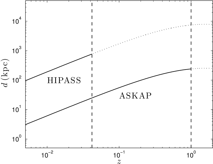
Figure 14: Physical size versus redshift for the 15.5 arcmin HIPASS beam and the upper-limit 30 arcsec beam expected for a future H i absorption survey using ASKAP. The solid lines indicate the physical scale of the beam within the redshift range indicated by the vertical dashed lines. At the higher redshifts available to an H i absorption survey using ASKAP, a 30 arcsec beam will be sensitive to the physical scales resolved by HIPASS.

We can use our results to estimate the number detections that might be achievable with the full ALFALFA survey. Considering a blind survey for associated absorption, conducted over 7000 deg² of the sky in the redshift range $0<cz<19\,000$ km^-1 (equating to a comoving volume of 0.0136 Gpc³), we use the local radio luminosity function of Mauch & Sadler (2007) to predict a total of 455 galaxies above a detection flux limit of 42 mJy (see Section 5.4 for an explanation of this limit). By simply applying our total detection rate from HIPASS, we predict approximately 10 detections of associated absorption, while applying the rate estimated for the pilot survey of Darling et al. (2011) yields approximately 16 (which is driven by the fractional increase in volume of the full survey). Since the ALFALFA survey probes higher redshifts than HIPASS, we expect that the detection rate amongst a radio flux density selected sample of galaxies will be higher, due to a decrease in the fraction of diffuse star-forming galaxies. We therefore predict a factor of 3–4 increase in the number of detections of associated absorption compared with what we have achieved in HIPASS.

Our results have positive implications for proposed all-sky absorption surveys on the precursor telescopes to the SKA, which will be able to probe the H i content of the Universe up to $z\approx 1$. In Fig. 14, we show that the physical scales to which HIPASS is sensitive in the local Universe are well matched at higher redshifts to the smaller beam sizes of the proposed First Large Absorption Survey in H i on the Australian Square Kilometre Array Pathfinder (ASKAP; Deboer et al. 2009). The HIPASS detections show that it will be possible to use ASKAP (with a spatial resolution of $d\sim 100$ kpc at $z\sim 0.5$) to detect strong absorption systems associated with compact AGN and nuclear starbursts at redshifts in the range $0.5<z<1.0$, probing an epoch of the Universe not yet explored by all-sky H i surveys.

Furthermore, our results indicate that such strong absorption systems detected in future all-sky surveys may well provide excellent targets for luminous H₂O megamaser detection at redshifts greater than 0.1, where so few have been discovered. Taylor et al. (2002) showed that for the sample of known H₂O megamaser galaxies at that time, the detection rate of H i absorption was greater than 42 per cent, higher than the typical rates achieved with targeted surveys of compact radio sources (see Allison et al. 2012a and references therein). Of the Seyfert 2 galaxies in which we have detected absorption, NGC 5793 has known H₂O megamaser emission from within a sub-pc disc around the AGN (Hagiwara et al., 1997), while 2MASX J13084201-2422581, although not detected, has been a candidate for several large-scale megamaser surveys (e.g. Braatz et al. 1996; Sato et al. 2005; Kondratko et al. 2006). VLBI studies at high spatial resolution show that the optically thick H i absorption in these galaxies probably arises within an edge-on disc on 100 pc scales. If dense molecular gas also exists on sub-pc scales, it is likely to be distributed as a circumnuclear disc that is similarly orientated and so generate significant amplification of H₂O emission towards us, thereby providing favourable conditions for the detection of megamasers at cosmological redshifts. We also note that radio-loud nuclear starburst galaxies such as Arp 220, which is host to multiple regions of OH megamaser emission within its double nuclei (Lonsdale et al., 1998; Rovilos et al., 2003), are likely to produce strong 1.6 GHz emission that can be detected in the wide frequency bands of these future H i surveys.

6 Summary

We have used archival data from HIPASS to search for H i 21 cm absorption within a sample of 204 nearby radio and star-forming galaxies, achieving a total detection rate of 2.0 per cent (4/204). Of these detections, three are found against compact radio sources (two AGN and a nuclear starburst), while the fourth is within the nearby large radio galaxy Centaurus A, which would not have been seen at larger redshifts. Although susceptible to low number statistics, the detection rate against just the morphologically compact radio sources (both AGN and nuclear starbursts) is higher than the total rate and closer to the typical values obtained from targeted surveys of compact sources.

In the case of 2MASX J13084201-2422581, the absorption line had not been previously detected in the literature, highlighting the serendipitous advantages of performing such a low-sensitivity all-sky survey for absorption. The 21 cm line profile is similar to that seen in other edge-on Seyfert 2 galaxies, indicating that the absorption may arise within a disc of H i gas on 100 pc scales. A follow-up observation with the ATCA at 10 arcsec spatial resolution demonstrates that all of the absorption detected in the HIPASS spectrum arises against the compact radio nucleus of this galaxy. The higher sensitivity and spectral resolution of the CABB system reveals the presence of a second blueshifted component that might signify a 200 km s^-1 outflow of neutral gas.

The detection rate we achieve with HIPASS is consistent with that found for the ALFALFA pilot survey carried out by Darling et al. (2011). We predict that the full ALFALFA survey will yield three to four times as many associated absorption systems as we have achieved with HIPASS, and that future all-sky absorption surveys at higher redshifts should yield many more new detections. HIPASS is sensitive to only the strongest absorption lines, which appear to be dominated by galaxies that exhibit edge-on discs of atomic gas and high columns of nuclear molecular gas that exhibit H₂O megamaser emission. We predict that such systems detected in future all-sky surveys have the potential to provide excellent targets for the detection of luminous H₂O megamaser emission close to the AGN, with the potential for direct measurement of black hole masses at cosmological redshifts (Miyoshi et al., 1995; Kuo et al., 2011) and independent determination of the Hubble Constant (Reid et al., 2013).

Appendix A Radio – optical source matches excluded from Sample 1

PKS 0056-572 (SUMSS J005846-565912, $S_{843}=479$ mJy) is reported by Johnston et al. (1995) as a quasar with a redshift of $z=0.018$; however, there is no apparent reference to the origin of this measurement and so we have excluded this object from our sample.

Fairall 0216 (SUMSS J005825-664841, $S_{843}=382$ mJy) is a galaxy pair with a redshift reported by Fairall (1980) of $z\approx 0.033$. However, Garilli et al. (1993) and Dalton et al. (1994) report a significantly higher redshift for one of the component galaxies ($z\sim 0.07$) and no redshift is given for the other. Given the potential unreliability of the original redshift measurement and confusion as to which component the radio source belongs, we exclude this object from our sample.

UM 310 (NVSS J011517-012705, $S_{1.4}=1080$ mJy) is reported in the 6dF GS catalogue to have a redshift of $z=0.014\,36$. However, the 6dF spectral features are weak and this estimate is inconsistent with the much higher value of $z=1.36$ measured by Lewis et al. (1979) based on the C iv $\lambda$1549 emission line. Since there is a high likelihood that this object is located outside of the HIPASS volume, we do not include it in our sample.

PKS 0131-522 (SUMSS J013305-520005, $S_{843}=366$ mJy) is reported by Johnston et al. (1995) as a quasar with a redshift of $z=0.02$; however, there is no apparent reference to the origin of this measurement and so we have excluded this object from our sample.

PKS 0208-512 (SUMSS J021046-510102, $S_{843}=3370$ mJy) has a redshift of $z=0.031\,56$ in the 6dF GS catalogue. However, this estimate is inconsistent with the significantly higher value of $z=1.003$ recorded in the quasar catalogue by Véron-Cetty & Véron 2010, and so we have excluded this object from our sample.

NGC 1310 (NVSS J032102-370604, $S_{1.4}=457$ mJy) is a spiral galaxy in the Fornax Cluster with a redshift of $0.006$ (Ferguson, 1989; Drinkwater et al., 2001). Its close proximity to bright extended radio emission from Fornax A, which is apparent upon visual inspection of SUMSS images, means that the integrated flux density recorded in the NVSS catalogue is likely to be unreliable. We have therefore excluded this object from our sample.

SNR J050854-684447 (SUMSS J050859-684333, $S_{843}=653$ mJy) is a flat-spectrum supernova remnant located within the Large Magellanic Cloud (Mathewson & Clarke, 1973).

6dF J0653599-415145 (SUMSS J065400-415144, $S_{843}=728$ mJy) has a measured redshift of $z=0.00$ in the 6dF GS catalogue. However, Sadler et al. (2014) find that the 6dF spectrum is contaminated by foreground Galactic nebular emission lines and their re-measured value of $z=0.0908$ puts the host galaxy well outside of the HIPASS volume.

PKS 0959-443 (MGPS-2 J100200-443806, $S_{843}=1790$ mJy) was originally measured by Wright et al. (1977) to have a redshift of $z=0.840$ based on quasar emission lines. After obtaining higher signal-to-noise data, Wright et al. (1979) found that the identification of the emission lines was incorrect and used the strong galaxy-type absorption system to measure a much lower redshift of $z=0.021$, re-classifying this object as a very compact nearby galaxy. Given the inconsistency of these redshift estimates, and that this source also lies in the Galactic plane, we have decided to exclude this from our sample. It should be noted that no 21 cm absorption line is seen towards this source either in the HIPASS data or in the literature.

GQ 1042+0747 (NVSS J104257+074850, $S_{1.4}=383$ mJy) was incorrectly matched with the background radio source. This dwarf spiral galaxy ($z=0.033\,21$) forms a close pair with the background quasar SDSS J104257.58+074850.5 ($z=2.665\,21$). Using 21 cm spectroscopy of the radio source, with the Green Bank Telescope (GBT), VLA and Very Long Baseline Array, Borthakur et al. (2010) detected intervening H i absorption in the foreground galaxy at $z=0.03310$. The GBT spectrum exhibits an absorption line with an FWHM of 3.6 km s^-1 and peak flux density of $\sim 18$ mJy, and is therefore consistent with this line not being detected in the HIPASS spectrum.

PKS 1221-42 (SUMSS J122343-423531, $S_{843}=3110$ mJy) was reported by Sadler et al. (2014) to have an incorrectly measured redshift of $z=0.0266$ in the 6dF GS catalogue, and that the correct value is $z=0.1706$ (Simpson et al., 1993; Johnston et al., 2005). Since this is outside of the HIPASS volume we have excluded the source from our sample.

PKS 1510-08 (NVSS J151250-090600, $S_{1.4}=2700$ mJy) is a quasar with a low redshift measurement of $z=0.006818$ reported in the 6dF GS catalogue. However, this estimate is inconsistent with the much higher value of $z=0.360$ measured by Thompson et al. (1990), and so we have excluded this source from our sample.

NGC 6210 (NVSS J164429+234759, $S_{1.4}=298$ mJy) is a planetary nebula ($cz=-36\,\mathrm{km}\,\mathrm{s}^{-1}$; Wilson 1953).

6dF J1716205-615706 (SUMSS J171620-615707, $S_{843}=258$ mJy) is identified as a star in the 6dF GS catalogue ($cz=-57\,\mathrm{km}\,\mathrm{s}^{-1}$; Jones et al. 2009).

PKS 1935-526 (SUMSS J193953-523039, $S_{843}=460$ mJy) is identified by Grandi (1983) as a dwarf galaxy with a single redshift measurement of $z=0.03$. Since there has been no further spectroscopic verification of this redshift measurement, we have excluded this source from our sample.

Appendix B Galaxies searched for associated H I absorption

Table 5: Properties of 204 galaxies searched for H i absorption in HIPASS. Right ascension and declination are given for the centre position used to extract the HIPASS spectrum. $cz_{\rm sys}$ and $\sigma_{cz}$ are the mean and uncertainty in the systemic redshift. $S_{843}$ and $\sigma_{\mathrm{843}}$ are the mean and uncertainty in the SUMSS/MGPS-2 flux density at 843 MHz (Mauch et al., 2003; Murphy et al., 2007). $S_{1.4}$ and $\sigma_{\mathrm{1.4}}$ are the mean and uncertainty in the NVSS total flux density at 1.4 GHz (Condon et al., 1998). $n_{843}$ and $n_{1.4}$ are the number of radio components in the NVSS and SUMSS/MGPS-2 images, respectively (van Velzen et al., 2012). Note that where available we have used the SUMSS/MGPS-2 and NVSS total flux densities compiled by van Velzen et al. (2012). $S_{\rm CHI}$ is the beam-weighted flux density extracted within a single HIPASS beamwidth from the 1.4 GHz CHIPASS compact source map (Calabretta et al. 2014). $S_{100\,\mu\mathrm{m}}$ and $S_{60\,\mu\mathrm{m}}$ are the 100 and 60 $\mu$m flux densities from the IRAS Faint Source, Point Source and Galaxy Catalogues (Beichman et al., 1988; Rice et al., 1988; Knapp et al., 1989; Moshir et al., 1992; Sanders et al., 2003). $K_{s}$ is the apparent $K_{s}$-band magnitude, within the 20 mag arcsec^-2 isophote, from the 2MASS (Skrutskie et al. 2006). $S_{\rm HI}$ is the integrated H i emission from HIPASS (Koribalski et al. 2004; Meyer et al. 2004; Wong et al. 2006). The radio morphology classifications are as those given by van Velzen et al. (2012), where p = point sources, g = star-forming galaxies, j = jets and lobes and u = unknown. The full version of this table is available online.

Name	RA	Dec.	$cz_{\rm sys}$	$\sigma_{cz}$	$z$ ref.	$S_{843}$	$\sigma_{843}$	$n_{843}$	$S_{1.4}$	$\sigma_{1.4}$	$n_{1.4}$	$S_{\rm CHI}$	$S_{100\,\mu\mathrm{m}}$	$S_{60\,\mu\mathrm{m}}$	$K_{s}$	$S_{\rm HI}$	Mor.	Sam.
	(J2000)		(km s-1)			(mJy)	(mJy)		(mJy)	(mJy)		(mJy)	(mJy)	(mJy)	(mag)	(Jy km s-1)
PKS 0000-550	00 03 10.63	-54 44 56.1	9767	24	Huchra et al. (2012)	1549	55	1	$-$	$-$	$-$	1050	$-$	$-$	10.30	$-$	j	1,2
ESO 193-G017	00 05 07.95	-50 49 18.1	11 169	45	Dressler & Shectman (1988)	281	10	1	$-$	$-$	$-$	93	$-$	$-$	11.00	$-$	j	1
IC 1531	00 09 35.54	-32 16 36.7	7632	45	Jones et al. (2009)	559	17	1	433	13	2	642	$-$	$-$	9.71	$-$	j	1,2
NGC 0025	00 09 59.28	-57 01 15.0	9465	32	Lauberts & Valentijn (1989)	619	24	1	$-$	$-$	$-$	445	$-$	$-$	9.98	$-$	j	1,2
NGC 0055	00 14 53.60	-39 11 47.9	129	2	Koribalski et al. (2004)	$-$	$-$	$-$	225	8	4	417	174 000	77 000	6.56	1990	g	2
NGC 0092	00 21 31.69	-48 37 29.3	3219	7	Meyer et al. (2004)	252	8	1	$-$	$-$	$-$	365	$-$	$-$	9.43	12	p	1
NGC 0193	00 39 18.58	+03 19 52.7	4414	15	Ogando et al. (2008)	$-$	$-$	$-$	1277	32	2	1710	$-$	$-$	9.34	$-$	j	2
NGC 0215	00 40 48.87	-56 12 50.7	8154	45	Jones et al. (2009)	310	10	2	$-$	$-$	$-$	334	$-$	$-$	9.96	$-$	j	2
NGC 0253	00 47 33.13	-25 17 19.7	243	2	Koribalski et al. (2004)	$-$	$-$	$-$	5572	121	8	5630	1290 000	968 000	3.82	694	g	1,2
UGC 00583	00 56 25.59	-01 15 44.9	11 461	3	Aihara et al. (2011)	$-$	$-$	$-$	1370	26	4	3240	$-$	$-$	10.60	$-$	j	2
NGC 0349	01 01 50.75	-06 47 59.3	5986	18	Ogando et al. (2008)	$-$	$-$	$-$	296	8	9	242	$-$	$-$	9.32	$-$	j	2
IC 1623B	01 07 47.56	-17 30 25.1	6087	45	Jones et al. (2009)	$-$	$-$	$-$	248	10	1	217	$-$	$-$	10.00	$-$	p	2

References

- Aaronson et al. (1980) Aaronson M., Mould J., Huchra J., 1980, ApJ, 237, 655
- Aihara et al. (2011) Aihara H. et al., 2011, ApJS, 193, 29
- Allison et al. (2012a) Allison J. R. et al., 2012a, MNRAS, 423, 2601
- Allison et al. (2013) Allison J. R., Curran S. J., Sadler E. M., Reeves S. N., 2013, MNRAS, 430, 157
- Allison et al. (2012b) Allison J. R., Sadler E. M., Whiting M. T., 2012b, PASA, 29, 221
- Anantharamaiah et al. (2000) Anantharamaiah K. R., Viallefond F., Mohan N. R., Goss W. M., Zhao J. H., 2000, ApJ, 537, 613
- Baan & Haschick (1995) Baan W. A., Haschick A. D., 1995, ApJ, 454, 745
- Baan et al. (1987) Baan W. A., van Gorkom J. H., Schmelz J. T., Mirabel I. F., 1987, ApJ, 313, 102
- Baars et al. (1977) Baars J. W. M., Genzel R., Pauliny-Toth I. I. K., Witzel A., 1977, A&A, 61, 99
- Barnes et al. (2005) Barnes D. G., Briggs F. H., Calabretta M. R., 2005, Radio Sci., 40, 5
- Barnes et al. (2001) Barnes D. G. et al., 2001, MNRAS, 322, 486
- Barvainis & Antonucci (2005) Barvainis R., Antonucci R., 2005, ApJ, 628, L89
- Becker et al. (1995) Becker R. H., White R. L., Helfand D. J., 1995, ApJ, 450, 559
- Beichman et al. (1988) Beichman C. A., Neugebauer G., Habing H. J., Clegg P. E., Chester T. J., 1988, Infrared Astronomical Satellite (IRAS) Catalogs and Atlases. Volume 1: Explanatory Supplement. NASA, Washington
- Borthakur et al. (2010) Borthakur S., Tripp T. M., Yun M. S., Momjian E., Meiring J. D., Bowen D. V., York D. G., 2010, ApJ, 713, 131
- Bothun & Schommer (1983) Bothun G. D., Schommer R. A., 1983, ApJ, 267, L15
- Braatz et al. (1996) Braatz J. A., Wilson A. S., Henkel C., 1996, ApJS, 106, 51
- Braun (2012) Braun R., 2012, ApJ, 749, 87
- Bregman et al. (1992) Bregman J. N., Hogg D. E., Roberts M. S., 1992, ApJ, 387, 484
- Briggs et al. (1997) Briggs F. H., Sorar E., Kraan-Korteweg R. C., van Driel W., 1997, PASA, 14, 37
- Calabretta et al. (2014) Calabretta M. R., Staveley-Smith L., Barnes D. G., 2014, PASA, 31, e007
- Catinella et al. (2008) Catinella B., Haynes M. P., Giovanelli R., Gardner J. P., Connolly A. J., 2008, ApJ, 685, L13
- Condon et al. (1991) Condon J. J., Anderson M. L., Helou G., 1991, ApJ, 376, 95
- Condon et al. (1998) Condon J. J., Cotton W. D., Greisen E. W., Yin Q. F., Perley R. A., Taylor G. B., Broderick J. J., 1998, AJ, 115, 1693
- Cooper et al. (1965) Cooper B. F. C., Price R. M., Cole D. J., 1965, Aust. J. Phys., 18, 589
- Curran (2012) Curran S. J., 2012, ApJ, 748, L18
- Curran et al. (2013) Curran S. J., Allison J. R., Glowacki M., Whiting M. T., Sadler E. M., 2013, MNRAS, 431, 3408
- Curran et al. (2007) Curran S. J., Darling J., Bolatto A. D., Whiting M. T., Bignell C., Webb J. K., 2007, MNRAS, 382, L11
- Curran & Whiting (2010) Curran S. J., Whiting M. T., 2010, ApJ, 712, 303
- Curran et al. (2011) Curran S. J., Whiting M. T., Tanna A., Bignell C., Webb J. K., 2011, MNRAS, 413, L86
- Dalton et al. (1994) Dalton G. B., Efstathiou G., Maddox S. J., Sutherland W. J., 1994, MNRAS, 269, 151
- Darling et al. (2011) Darling J., Macdonald E. P., Haynes M. P., Giovanelli R., 2011, ApJ, 742, 60
- Deboer et al. (2009) Deboer D. R. et al., 2009, Proc. IEEE, 97, 1507
- Devereux & Eales (1989) Devereux N. A., Eales S. A., 1989, ApJ, 340, 708
- Dickey (1982) Dickey J. M., 1982, ApJ, 263, 87
- Dickey (1986) Dickey J. M., 1986, ApJ, 300, 190
- Dressler & Shectman (1988) Dressler A., Shectman S. A., 1988, AJ, 95, 284
- Drinkwater et al. (2001) Drinkwater M. J., Gregg M. D., Holman B. A., Brown M. J. I., 2001, MNRAS, 326, 1076
- Fairall (1980) Fairall A. P., 1980, MNRAS, 192, 389
- Ferguson (1989) Ferguson H. C., 1989, AJ, 98, 367
- Feroz & Hobson (2008) Feroz F., Hobson M. P., 2008, MNRAS, 384, 449
- Feroz et al. (2009) Feroz F., Hobson M. P., Bridges M., 2009, MNRAS, 398, 1601
- Field (1958) Field G. B., 1958, Proc. IRE, 46, 240
- Field (1959) Field G. B., 1959, ApJ, 129, 536
- Freudling et al. (2011) Freudling W. et al., 2011, ApJ, 727, 40
- Gallimore et al. (1999) Gallimore J. F., Baum S. A., O’Dea C. P., Pedlar A., Brinks E., 1999, ApJ, 524, 684
- Gardner & Whiteoak (1986) Gardner F. F., Whiteoak J. B., 1986, MNRAS, 221, 537
- Gardner et al. (1992) Gardner F. F., Whiteoak J. B., Norris R. P., Diamond P. J., 1992, MNRAS, 258, 296
- Garilli et al. (1993) Garilli B., Maccagni D., Tarenghi M., 1993, A&A, 100, 33
- Garwood et al. (1987) Garwood R. W., Dickey J. M., Helou G., 1987, ApJ, 322, 88
- Giovanelli et al. (2005) Giovanelli R. et al., 2005, AJ, 130, 2598
- Grandi (1983) Grandi S. A., 1983, MNRAS, 204, 691
- Hagiwara et al. (1997) Hagiwara Y., Kohno K., Kawabe R., Nakai N., 1997, PASJ, 49, 171
- Hambly et al. (2001) Hambly N. C. et al., 2001, MNRAS, 326, 1279
- Harris et al. (2010) Harris G. L. H., Rejkuba M., Harris W. E., 2010, PASA, 27, 457
- Helou et al. (1985) Helou G., Soifer B. T., Rowan-Robinson M., 1985, ApJ, 298, L7
- Hibbard et al. (2000) Hibbard J. E., Vacca W. D., Yun M. S., 2000, AJ, 119, 1130
- Huchra et al. (2012) Huchra J. P. et al., 2012, ApJS, 199, 26
- Huchra et al. (1999) Huchra J. P., Vogeley M. S., Geller M. J., 1999, ApJS, 121, 287
- Impellizzeri et al. (2008) Impellizzeri C. M. V., McKean J. P., Castangia P., Roy A. L., Henkel C., Brunthaler A., Wucknitz O., 2008, Nature, 456, 927
- Israel (1998) Israel F. P., 1998, A&AR, 8, 237
- Jarrett et al. (2000) Jarrett T. H., Chester T., Cutri R., Schneider S., Skrutskie M., Huchra J. P., 2000, AJ, 119, 2498
- Jenkins (1983) Jenkins C. R., 1983, MNRAS, 205, 1321
- Johnston et al. (2005) Johnston H. M., Hunstead R. W., Cotter G., Sadler E. M., 2005, MNRAS, 356, 515
- Johnston et al. (1995) Johnston K. J. et al., 1995, AJ, 110, 880
- Jones et al. (2009) Jones D. H. et al., 2009, MNRAS, 399, 683
- Kanekar et al. (2007) Kanekar N., Chengalur J. N., Lane W. M., 2007, MNRAS, 375, 1528
- Knapp et al. (1989) Knapp G. R., Guhathakurta P., Kim D.-W., Jura M. A., 1989, ApJS, 70, 329
- Kondratko et al. (2006) Kondratko P. T. et al., 2006, ApJ, 638, 100
- Koribalski (2012) Koribalski B. S., 2012, PASA, 29, 359
- Koribalski et al. (2004) Koribalski B. S. et al., 2004, AJ, 128, 16
- Kuo et al. (2011) Kuo C. Y. et al., 2011, ApJ, 727, 20
- Lah et al. (2009) Lah P. et al., 2009, MNRAS, 399, 1447
- Lauberts & Valentijn (1989) Lauberts A., Valentijn E. A., 1989, The Surface Photometry Catalogue of the ESO-Uppsala Galaxies. European Southern Observatory, Garching
- Lewis et al. (1979) Lewis D. W., MacAlpine G. M., Weedman D. W., 1979, ApJ, 233, 787
- Lonsdale et al. (1998) Lonsdale C. J., Diamond P. J., Smith H. E., Lonsdale C. J., 1998, ApJ, 493, L13 (erratum 494, L239)
- Mahony et al. (2013) Mahony E. K., Morganti R., Emonts B. H. C., Oosterloo T. A., Tadhunter C., 2013, MNRAS, 435, L58
- Mathewson & Clarke (1973) Mathewson D. S., Clarke J. N., 1973, ApJ, 180, 725
- Mauch et al. (2003) Mauch T., Murphy T., Buttery H. J., Curran J., Hunstead R. W., Piestrzynski B., Robertson J. G., Sadler E. M., 2003, MNRAS, 342, 1117
- Mauch & Sadler (2007) Mauch T., Sadler E. M., 2007, MNRAS, 375, 931
- Meyer et al. (2004) Meyer M. J. et al., 2004, MNRAS, 350, 1195
- Mirabel (1982) Mirabel I. F., 1982, ApJ, 260, 75
- Miyoshi et al. (1995) Miyoshi M., Moran J., Herrnstein J., Greenhill L., Nakai N., Diamond P., Inoue M., 1995, Nature, 373, 127
- Moore et al. (1999) Moore C. B., Carilli C. L., Menten K. M., 1999, ApJ, 510, L87
- Morganti et al. (2013) Morganti R., Fogasy J., Paragi Z., Oosterloo T., Orienti M., 2013, Science, 341, 1082
- Morganti et al. (2011) Morganti R., Holt J., Tadhunter C., Ramos Almeida C., Dicken D., Inskip K., Oosterloo T., Tzioumis T., 2011, A&A, 535, A97
- Morganti et al. (2008) Morganti R., Oosterloo T., Struve C., Saripalli L., 2008, A&A, 485, L5
- Morganti et al. (2001) Morganti R., Oosterloo T. A., Tadhunter C. N., van Moorsel G., Killeen N., Wills K. A., 2001, MNRAS, 323, 331
- Morganti et al. (2005) Morganti R., Tadhunter C. N., Oosterloo T. A., 2005, A&A, 444, L9
- Moshir et al. (1992) Moshir M. et al., 1992, Explanatory Supplement to the IRAS Faint Source Survey, version 2, JPL D-10015 8/92. California Institute of Technology, Pasadena
- Mundell et al. (2001) Mundell C. G., Ferruit P., Pedlar A., 2001, ApJ, 560, 168
- Murphy et al. (2007) Murphy T., Mauch T., Green A., Hunstead R. W., Piestrzynska B., Kels A. P., Sztajer P., 2007, MNRAS, 382, 382
- Norris (1988) Norris R. P., 1988, MNRAS, 230, 345
- Ogando et al. (2008) Ogando R. L. C., Maia M. A. G., Pellegrini P. S., da Costa L. N., 2008, AJ, 135, 2424
- Pihlström et al. (2000) Pihlström Y. M., Conway J. E., Booth R. S., Diamond P. J., Koribalski B. S., 2000, A&A, 357, 7
- Purcell & Field (1956) Purcell E. M., Field G. B., 1956, ApJ, 124, 542
- Reid et al. (2013) Reid M. J., Braatz J. A., Condon J. J., Lo K. Y., Kuo C. Y., Impellizzeri C. M. V., Henkel C., 2013, ApJ, 767, 154
- Rice et al. (1988) Rice W., Lonsdale C. J., Soifer B. T., Neugebauer G., Kopan E. L., Lloyd L. A., de Jong T., Habing H. J., 1988, ApJS, 68, 91
- Roberts (1970) Roberts M. S., 1970, ApJ, 161, L9
- Rovilos et al. (2003) Rovilos E., Diamond P. J., Lonsdale C. J., Lonsdale C. J., Smith H. E., 2003, MNRAS, 342, 373
- Sadler et al. (2014) Sadler E. M., Ekers R. D., Mahony E. K., Mauch T., Murphy T., 2014, MNRAS, 438, 796
- Sakamoto et al. (1999) Sakamoto K., Scoville N. Z., Yun M. S., Crosas M., Genzel R., Tacconi L. J., 1999, ApJ, 514, 68
- Sanders et al. (2003) Sanders D. B., Mazzarella J. M., Kim D.-C., Surace J. A., Soifer B. T., 2003, AJ, 126, 1607
- Sarma et al. (2002) Sarma A. P., Troland T. H., Rupen M. P., 2002, ApJ, 564, 696
- Sato et al. (2005) Sato N., Yamauchi A., Ishihara Y., Sorai K., Kuno N., Nakai N., Balasubramanyam R., Hall P., 2005, PASJ, 57, 587
- Sault et al. (1995) Sault R. J., Teuben P. J., Wright M. C. H., 1995, in ASP Conf. Ser., Vol. 77, Astronomical Data Analysis Software and Systems IV, Shaw R. A., Payne H. E., & Hayes J. J. E., ed., Astron. Soc. Pac., San Francisco, p. 433
- Simpson et al. (1993) Simpson C., Clements D. L., Rawlings S., Ward M., 1993, MNRAS, 262, 889
- Skilling (2004) Skilling J., 2004, in AIP Conf. Ser., Vol. 735, Bayesian Inference and Maximum Entropy methods in Science and Engineering, Fischer R., Preuss R. & Toussaint U. V., ed., Am. Inst. Phys., New York, p. 395
- Skrutskie et al. (2006) Skrutskie M. F. et al., 2006, AJ, 131, 1163
- Soifer et al. (1989) Soifer B. T., Boehmer L., Neugebauer G., Sanders D. B., 1989, AJ, 98, 766
- Struve & Conway (2010) Struve C., Conway J. E., 2010, A&A, 513, A10
- Struve et al. (2010) Struve C., Oosterloo T. A., Morganti R., Saripalli L., 2010, A&A, 515, A67
- Tanna et al. (2013) Tanna A., Curran S. J., Whiting M. T., Webb J. K., Bignell C., 2013, ApJ, 772, L25
- Taylor et al. (2002) Taylor G. B., Peck A. B., Henkel C., Falcke H., Mundell C. G., O’Dea C. P., Baum S. A., Gallimore J. F., 2002, ApJ, 574, 88
- Taylor (2005) Taylor M. B., 2005, in ASP Conf. Ser., Vol. 347, Astronomical Data Analysis Software and Systems XIV, Shopbell P., Britton M., Ebert R., eds., Astron. Soc. Pac., San Francisco, p. 29
- Thompson et al. (1990) Thompson D. J., Djorgovski S., de Carvalho R., 1990, PASP, 102, 1235
- Tingay et al. (2003) Tingay S. J., Jauncey D. L., King E. A., Tzioumis A. K., Lovell J. E. J., Edwards P. G., 2003, PASJ, 55, 351
- Tully & Fisher (1977) Tully R. B., Fisher J. R., 1977, A&A, 54, 661
- Uson et al. (1991) Uson J. M., Bagri D. S., Cornwell T. J., 1991, Phys. Rev. Lett., 67, 3328
- van der Hulst et al. (1983) van der Hulst J. M., Golisch W. F., Haschick A. D., 1983, ApJ, 264, L37
- van Velzen et al. (2012) van Velzen S., Falcke H., Schellart P., Nierstenhöfer N., Kampert K.-H., 2012, A&A, 544, A18
- Verheijen et al. (2010) Verheijen M. A. W. et al., 2010, in ISKAF2010 Science Meeting, van Leeuwen J., ed., Proc. Sci.
- Vermeulen et al. (2003) Vermeulen R. C. et al., 2003, A&A, 404, 861
- Véron-Cetty & Véron (2010) Véron-Cetty M.-P., Véron P., 2010, A&A, 518, A10
- Wall & Peacock (1985) Wall J. V., Peacock J. A., 1985, MNRAS, 216, 173
- Wegner et al. (2003) Wegner G. et al., 2003, AJ, 126, 2268
- White et al. (1997) White R. L., Becker R. H., Helfand D. J., Gregg M. D., 1997, ApJ, 475, 479
- Whiteoak & Gardner (1971) Whiteoak J. B., Gardner F. F., 1971, ApJ, 8, 57
- Whiting (2012) Whiting M. T., 2012, MNRAS, 421, 3242
- Williams & Brown (1983) Williams B. A., Brown R. L., 1983, AJ, 88, 1749
- Wilson (1953) Wilson R. E., 1953, General Catalogue of Stellar Radial Velocities. Carnegie Institution of Washington, Washington
- Wilson et al. (2011) Wilson W. E. et al., 2011, MNRAS, 416, 832
- Wolfe & Burbidge (1975) Wolfe A. M., Burbidge G. R., 1975, ApJ, 200, 548
- Wong et al. (2006) Wong O. I. et al., 2006, MNRAS, 371, 1855
- Wright et al. (1977) Wright A. E., Jauncey D. L., Peterson B. A., Condon J. J., 1977, ApJ, 211, L115
- Wright et al. (1979) Wright A. E., Peterson B. A., Jauncey D. L., Condon J. J., 1979, ApJ, 229, 73
- Zwaan et al. (2004) Zwaan M. A. et al., 2004, MNRAS, 350, 1210